1
THE POLLUTION INDEX PROGRAM
USER’S MANUAL
AND
TUTORIAL
Kedar Telang and Ralph W. Pike
March 1, 2001
Copyright 2001
Mineral Processing Research Institute
Louisiana State University
Baton Rouge, LA- 70803
TABLE OF CONTENTS
Disclaimer . . . . . . . . . . . . . . . . . . . . . . . . . . . . . . . . . . . . . . . . . . . . . . . . . . . . . . . . . . . . . . . . . . . . i
Installation . . . . . . . . . . . . . . . . . . . . . . . . . . . . . . . . . . . . . . . . . . . . . . . . . . . . . . . . . . . . . . . . . . . . i
Introduction . . . . . . . . . . . . . . . . . . . . . . . . . . . . . . . . . . . . . . . . . . . . . . . . . . . . . . . . . . . . . . . . . . . 1
Methodology . . . . . . . . . . . . . . . . . . . . . . . . . . . . . . . . . . . . . . . . . . . . . . . . . . . . . . . . . . . . . . . . . . 1
The Environmental Impact Theory . . . . . . . . . . . . . . . . . . . . . . . . . . . . . . . . . . . . . . . . . . . . . . . . . . 1
Pollution Indices . . . . . . . . . . . . . . . . . . . . . . . . . . . . . . . . . . . . . . . . . . . . . . . . . . . . . . . . . . . . . . . . 3
Tutorial Session . . . . . . . . . . . . . . . . . . . . . . . . . . . . . . . . . . . . . . . . . . . . . . . . . . . . . . . . . . . . . . . . 6
General Information . . . . . . . . . . . . . . . . . . . . . . . . . . . . . . . . . . . . . . . . . . . . . . . . . . . . . . . . . . . . 14
Acknowledgments . . . . . . . . . . . . . . . . . . . . . . . . . . . . . . . . . . . . . . . . . . . . . . . . . . . . . . . . . . . . . 14
References . . . . . . . . . . . . . . . . . . . . . . . . . . . . . . . . . . . . . . . . . . . . . . . . . . . . . . . . . . . . . . . . . . . 16
LIST OF FIGURES
Figure 1
Process Flow Diagram for the MEK Process . . . . . . . . . . . . . . . . . . . . . . . . . . . . . . 7
Figure 2
Welcome Window . . . . . . . . . . . . . . . . . . . . . . . . . . . . . . . . . . . . . . . . . . . . . . . . . . 9
Figure 3
Open Model Dialog Box . . . . . . . . . . . . . . . . . . . . . . . . . . . . . . . . . . . . . . . . . . . . 10
Figure 4
Stream Data . . . . . . . . . . . . . . . . . . . . . . . . . . . . . . . . . . . . . . . . . . . . . . . . . . . . . . 11
Figure 5
Pollution Indices . . . . . . . . . . . . . . . . . . . . . . . . . . . . . . . . . . . . . . . . . . . . . . . . . . . 13
Figure 6
WAR Algorithm . . . . . . . . . . . . . . . . . . . . . . . . . . . . . . . . . . . . . . . . . . . . . . . . . . . 15
DISCLAIMER
Mineral Processing Research Institute(MPRI) makes no warranties, express or implied, including
without limitation the implied warranties of merchantability and fitness for particular purpose, regarding the
MPRI software. MPRI does not warrant, guarantee or make any representation regarding the use or the
results of the use of the MPRI software in terms of its correctness, accuracy, reliability, currentness or
otherwise. The entire risk as to the results and performance of the MPRI software is assumed by you.
In no event will MPRI, its director, officers, employees or agents be liable to you for any
consequential, incidental or indirect damages (including damage for loss of business profits, business
interruption, loss of business information, and the like) arising out of the use or inability to use the MPRI
software even if MPRI has been advised of the possibility of such damages.
INSTALLATION
The PollutionIndex Program must be installed under Windows 95 or Windows NT. The procedure
to install the program is described as following:
1)
Insert CD-ROM in CD-ROM Drive and run the “pollinstall.exe” program.
2)
The default destination directory is “C:\Program Files\pollution” into which the program will be
copied when the setup program is run.
3)
The short cut will be created Under start Programs Advanced Process Analysis.
4)
Run the program “pollution.exe” in the installation directory.
i
1
Introduction
Cost minimization has traditionally been the objective of chemical process design. However,
growing environmental awareness now demands process technologies that minimize or prevent production
of wastes. The development of such environmentally benign processes requires a tool which can perform
a quantitative measurement of the pollution impact of a process.
The pollution index program is a pollution prevention and measurement module, which can be used
to assess the environmental impact of chemical and refinery processes. It is based on the pollution index
methodology of EPA (Hilaly and Sikdar, 1995). This approach defines pollution indices which can be used
to compare the performance of different chemical processes.
Methodology
There is a wealth of information on methods for pollution prevention for chemical and refinery
processes. Some methods currently being developed are the Waste Reduction Algorithm (WAR) by Hilaly
and Sikdar, (1995), the Environmental Impact Theory by Cabezas et al., (1997), the Clean Process
Advisory System (CPAS) by Baker et.al.(1995) and the Mass Exchange Network Methodology by
Papalexandri et al.(1994).
The Pollution Index Program uses the Waste Reduction Algorithm (WAR). The WAR algorithm
can be used to minimize waste in the design of new processes as well as in the modification of existing
processes. It is based on the generic pollution balance of a process flow diagram as given below .
Pollution Accumulation = Pollution Inputs + Pollution Generation - Pollution Output.
(1)
In the WAR algorithm, a quantity called as the 'Pollution Index' is defined to measure the waste
generation in a process. This index also allows comparison of pollution production of different processes.
The Environmental Impact Theory (Cabezas et. al., 1997)
This theory is a generalization of the WAR algorithm which discusses the methodology for
evaluating potential environmental impacts and illustrating its use in the design and modification of chemical
processes. The environmental impacts of a chemical process are generally caused by the energy and
material that the process takes from and emits to the environment. The potential environmental impact is
2
a conceptual quantity that can not be measured. However, it can be calculated from related measurable
quantities.
The generic pollution balance equation of the WAR algorithm (Eqn. 1) is now applied to the
conservation of potential environmental impact in a process. The flow of impact in and out of the process
is related to mass and energy flows but is not equivalent to them. The conservation equation can be written
as
dIsys & &
= Iin − Iout + I&gen
dt
(2)
In the conservation equation, Isys is the potential environmental impact content inside the process, Iin is the
input rate of impact, Iout is the output rate of impact and Igen is the rate of impact generation inside the
process by chemical reactions or other means.
Application of this equation to chemical processes requires an expression that relates the conceptual
impact quantity to measurable quantities. This can be written as
I&i =
∑
j
I&j ( i ) =
∑
j
M& j ( i ) ∑ xkjΨ k
(3)
k
where Ii is the total impact flow in the input or the output. The sum over j is taken over all the process
streams. For each stream, a sum is taken over all the chemicals where Mj is the mass flow rate of the
stream j and xkj is the mass fraction of chemical k in that stream. Qk is the characteristic potential impact
of chemical k.
The process streams are divided into three types: Input, Product and Non-product. All nonproduct
NP
I&gen
= I&outNP − I&inNP
streams
are considered as
containing pollutants, and all product
streams are considered to have zero potential impact. This assumption is made because the objective of
the methodology is to reduce the impact and amount of waste materials released into the environment.
Since the product streams are not released into the environment, they are considered to have zero potential
impact.
3
The potential environmental impact of a chemical species is calculated using the following
expression.
Ψk = ∑
l
l
Ψ ks ,l
(4)
where the sum is taken over the categories of environmental impact. " l is the relative weighting factor for
impact of type l independent of chemical k. Qk,ls is the potential environmental impact of chemical k for
impact of type l.
There are nine different categories of impact. These can be subdivided into four physical potential
impacts (acidification, greenhouse enhancement, ozone depletion and photochemical oxidant formation),
three human toxicity effects (air, water and soil) and two ecotoxicity effects ( aquatic and terrestrial). The
relative weighting factor " l allows the above expression for the impact to be customized to specific or local
conditions. The suggested procedure is to initially set all the " ls to one and then allow the user to vary them
according to local needs.
To quantitatively describe the pollution impact of a process, the conservation equation is used to
define two categories of Impact Indices. The first category is based on generation of potential impact within
the process. These are useful in addressing the questions related to the internal environmental efficiency of
the process plant, i.e., the ability of the process to produce desired products while creating a minimum of
environmental impact. The second category measures the potential impact emitted by the process. This is
a measure of the external environmental efficiency of the process, i.e., the ability to produce the desired
products while inflicting on the environment a minimum of impact.
Within each of these categories, three types of indices are defined. In the first category (generation),
the three indices are as follows.
1.
NP
I&gen
measures the total rate at which the process generates potential environmental impact due
to nonproducts. This can be calculated by subtracting the input rate of impact from the output rate of impact
as shown in the following equation.
(5)
NP
and I&inNP can be calculated using equation 3.
I&out
4
NP
NPNP
I$gen
I&gen
I&out −measures
I&inNP the potential impact created by all
NP
$I gen
=
=
&
P
∑ p
∑ P&p nonproducts in manufacturing a unit
2.
p
p
mass of all the products.
It is
calculated by dividing index 1 by the rate at which the process outputs products. This is shown in the
following equation.
(6)
where
∑ P&
p
is the total rate of output of products.
p
3.
$ NP measures the mass efficiency of the process, i.e., the ratio of mass converted to an
M
gen
undesirable form to mass converted to a desirable form. It is calculated from index 2 by assigning
a value of 1 to the potential impacts of all non-products. This is shown in the following equation.
NP
M$ gen
=
∑j M& (j out ) ∑k x kjNP − ∑j M& (j in) ∑k x kjNP
∑p P&p
(7)
The indices in the second category (emission) are as follows.
4.
NP
I&out
measures the total rate at which the process outputs potential environmental impacts due
to non-products. It is calculated using equation 3.
5.
NP
I$out
measures the potential impact emitted in manufacturing a unit mass of all the products.
It is
calculated by dividing index 4 by the rate at which the process outputs products This is shown
in the
following equation.
& NP
$I outNP = I out
∑ P&p
p
(8)
5
6.
$ NP measures the amount of pollutant mass emitted in manufacturing a unit mass of product. It
M
out
is calculated from index 5 by assigning a value of 1 to the potential impacts of all non-products. This is
shown in the following equation.
M$ outNP =
∑j M& (j out ) ∑k xkjNP
∑p P&p
(9)
The first category of indices (indices 1,2 and 3) categorizes generation of potential environmental
impact within a process. These indices are most useful in addressing questions related to the internal
environmental efficiency of the process plant. Smaller the values of these indices, more environmentally
efficient is the process. The second category of indices (indices 4,5 and 6) categorizes emission of potential
impact within a process. These are useful in questions related to external environmental efficiency of the
process. Indices 1 and 4 can be used for comparison of different designs on an absolute basis whereas the
other indices can be used to compare designs independent of the plant size.
In addition to these indices for the process, pollution indices can be defined for the individual
streams also. Higher the pollution index of a stream, higher is the pollution impact of that stream on the
environment. Since all product streams are considered to have zero potential impact, their pollution index
values are zero. The pollution index value for a stream j can be calculated using the following equation.
&
I& j = M
j
∑
xkjΨ k
(10)
k
where Mj is the mass flow rate of the stream j, xkj is the mass fraction of chemical k in that stream and
Qk is the characteristic potential impact of chemical k.
6
Tutorial Session:
To illustrate the use of WAR Algorithm and the working of the Pollution Index Program, a small
tutorial problem (Cabezas et. al., 1997) is given below. The process is of production of methyl ethyl ketone
(MEK) from secondary butyl alcohol (SBA). This is a typical chemical engineering process with several
unit processes such as reactors, separators, mixers etc. and is thus ideally suited for the purpose of this
illustration.
The process flow diagram for the above process is shown in Figure 1. SBA is fed to a hydrogen
scrubber where the feed SBA scrubs residual MEK from the hydrogen stream. The SBA feed is then
pumped up to the reaction pressure and heated to the reaction temperature. This feed then enters the
reactor. The output of the reactor is then sent to a heat exchanger where it is partially condensed. The
mixture of MEK, SBA and hydrogen is cooled further and sent to a separator where the hydrogen is
flashed off. The hydrogen is then scrubbed and the liquid phase is then sent to the MEK purification system
where it is separated into product MEK and waste SBA.
The mass flow rates (kg/hr) of the input and output streams are given in Table 1, and the potential
environmental impact scores for these chemicals are given in Table 2 from Cabezas et al. (1997).
Table 1 Mass Flowrates of Input and Output Streams for the MEK Process
Stream Number
1
2
3
4
5
SBA
3362
19
3
2670
1
MEK
0
0
567
13
71
H2O
8
0
0
0
8
H2
0
18
0
0
0
Table 2 Potential Environmental Impact Scores for Chemicals in the MEK Process.
Qj,l ( impact / kg )
H2
MEK
SBA
H2O
0
0.42
0.00041
0
7
1
2
Feed SBA
By-prod H2
Cooler
Reactor
Heater
Pump
H2O-MEK
4
3
Product MEK
Crude MEK
Waste SBA
5
Figure 1: Process Flow Diagram for the MEK Process. (Cabezas et al., 1997)
8
Now that we have all the necessary data, let us use the Pollution Index Program for this problem.
On running the program, the ‘Welcome Window’ as shown in Figure 2 appears on the screen. It gives a
short description of the program’s function and the Potential Environmental Impact theory. It asks the user
to choose either a new model or an existing model. We will choose the ‘New Model’ option. ( For an
existing model, the program shows the ‘Open Model’ dialog box shown in Figure 3)
Next, the program shows the ‘Stream Data’ form which is given in Figure 4. Since we have chosen
a New model, all the data fields will be initially empty.
The table at the top left corner shows the list of streams in the model. New streams can be added
by first entering the necessary stream data and then clicking the ‘Add Stream to list’ button. The necessary
stream data includes the stream name, the component data and the stream type. The component data
includes the component name and its flowrate. The component flowrates can also be specified in terms of
the mass fractions along with the total mass flowrate of the stream.
Since we have the data in terms of mass flowrates, we do not need to specify the total flowrate of
any stream. So, let us enter the data for the stream number 1. In the box for the stream name, let us enter
str1. (We will name all of our streams for this problem as str1, sr2 and so on). We will click the ‘Mass
flowrates of components’ option in the ‘Specify’ box. In the Components Data table, we will enter the two
components: H2O and SBA and their corresponding flowrates. Other components of the system which are
not present in this stream need not be entered.
In accord with the Environmental Impact Theory, the process streams are divided into three
categories: Input, Product and Non-Product. Str1 is an input stream. So, in the Stream Type list, we will
choose ‘Input’. Having entered all the information for this stream, we can now click the ‘Add stream to list’
button. The stream now gets added to the Stream List table at the top. In this manner, we can add all the
five streams to our model.
The list at the right hand top of the form shows the list of all the components in the process.
Whenever, a new component is added to the model, it is automatically added to this list. Each of these
components has Specific Environmental Impact Potentials, Qsj,l for each of the nine different categories
of impacts. The user has to click on the component name in the list and then enter the Qsj,l values in the
table. All the impact potentials have a default value of zero.
So, let us click on SBA in the ‘Choose component’ list and enter the value of 0.00041 in the first
9
impact type. Also, click on MEK and enter 0.42.
Figure 2: Welcome Window
10
Figure 3: Open Model Dialog Box
11
Figure 4: Stream Data
12
Also, the user has to enter the Relative Weighting Factors (" l ) for the process. In accordance with
the theory, all the " l s are initialized to one. For this problem, we will retain these default values.
To modify the information for any stream, the user simply has to click on that stream in the list, and
the data for that stream appears in the boxes. The user can make the required changes and click the
‘Update Stream Information’ button. Similarly, to delete a stream, the user has to select the stream first and
press the ‘Delete Stream’ button.
All of this model information is written to a temporary buffer. At any time, the user can save the
model by choosing the ‘Save’ option in the menu. Let us save our model in a file called ‘example.mdb’.
( The model is stored as a Microsoft Access database file. So, it must have the ‘.mdb’ extension.)
Now that we have entered and saved the model, the ‘Calculate Indices’ button can be clicked to
view the values of the six pollution indices defined earlier. On clicking this button, the program uses the data
entered by the user to evaluate these indices using equations 5-9. It then displays on the screen the
‘Pollution Indices’ form which shows the results of these evaluations. This form is shown in Figure 5. The
column on the left-hand side shows the indices based on the generation of potential environmental impact
and the right-hand side column shows the indices based on the emission of environmental impact. Each
index is accompanied by a Help button. Clicking the ‘Help’ displays more information about that particular
index at the bottom of the screen. The results for this problem are given in Table 3.
Table 3 Results for the MEK process.
Index Type
Value
Units
Based on Generation of Potential Environmental Impact
Total rate of Impact Generation
35.00448
Impact / hr
Specific Impact Generation
0.061411
Impact / kg product
-1
kg pollutants / kg products
Total rate of Impact Emission
36.3829
Impact / hr
Specific Impact Emission
0.063827
Impact / kg product
Rate of Emission of pollutants / product
4.91228
kg pollutants / kg products
Rate of Generation of pollutants / product
Based on Emission of Potential Environmental Impact
13
Figure 5: Pollution Indices
14
Let us click the ‘Show the WAR algorithm’ button which will display the ‘WAR Algorithm’
window shown in Figure 6. In this figure, the table on the left side shows the pollution index values for the
individual streams. These values are obtained by applying equation 10 to all the process streams. A
comparison of these values can help in identifying streams with high pollutant content.
The pollution index values for the individual streams in the MEK process are given in Table 4. We
can see that stream 5 has a very high pollutant content followed by stream 4. Stream 3 has no pollutants
because it is a product stream. The form also shows the important steps of WAR Algorithm which gives
a systematic way of approaching the waste minimization problem. Process modifications should be made
to reduce the pollutant contents of streams 4 and 5. Clicking the ‘Back’ button will bring us back to the
‘Indices’ form.
Table 4 Pollution Index Values for Streams in the MEK Process
str1
str2
str3
str4
str5
1.37
0.00779
0
6.55
29.8
To make modifications in our model, we can click the ‘Back to Stream Data’ button which
will again display the ‘Stream Data’ window. We can now add and delete streams, change data for existing
streams, change the Impact Potentials for the components etc. and again click the ‘Calculate Indices’
button to see the results for the modified model. In order to save the changes to the model, the ‘Save’
option on the menu must be used.
Thus, we can make changes in the model and see the effect on the pollution indices by
going back and forth in these windows. The ‘Exit’ button in the menu will quit the application.
General Information:
The pollution index program is written using Visual Basic 5.0. It uses Microsoft Access 97 as the
database.
15
Acknowledgments:
The support of Gulf Coast Hazardous Substance Research Center is gratefully acknowledged.
16
Figure 6: WAR Algorithm
17
References:
Hilaly, A. K., Sikdar, S. K., 1994, PollutionBalance: New Methodology for Minimizing Waste Production
in Manufacturing Processes., J.Air and Waste Manage.Assoc., 44, 1303.
Cabezas, H., Bare, J. C., Mallick, S.K., 1997, Pollution Prevention with Chemical Process Simulators:
the Generalized Waste Reduction (WAR) Algorithm, Computers chem Engg, Vol. 21, pp S305310.
Baker, James R., R. J. Hossli, M. M. Zanoni and P. P. Radeciki, 1995, “A Demonstration Version of the
Clean Process Advisory System,” Paper No. 8a, AIChE Summer National Meeting, Boston,
Massachusetts.