Download GAPS/CoGAPS Users Manual

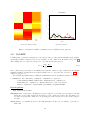
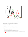
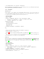
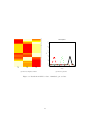
GAPS/CoGAPS Users Manual
Elana J. Fertig
email: [email protected]
September 2, 2011
Contents
1 Introduction
2
2 Installation Instructions
2.1 GAPS-JAGS . . . . .
2.1.1 Unix / MAC .
2.1.2 Windows . . .
2.2 CoGAPS . . . . . . .
2.2.1 Unix / Mac . .
2.2.2 Windows . . .
.
.
.
.
.
.
.
.
.
.
.
.
.
.
.
.
.
.
.
.
.
.
.
.
.
.
.
.
.
.
.
.
.
.
.
.
.
.
.
.
.
.
.
.
.
.
.
.
.
.
.
.
.
.
.
.
.
.
.
.
.
.
.
.
.
.
.
.
.
.
.
.
.
.
.
.
.
.
.
.
.
.
.
.
.
.
.
.
.
.
.
.
.
.
.
.
.
.
.
.
.
.
.
.
.
.
.
.
.
.
.
.
.
.
.
.
.
.
.
.
.
.
.
.
.
.
.
.
.
.
.
.
.
.
.
.
.
.
.
.
.
.
.
.
.
.
.
.
.
.
.
.
.
.
.
.
.
.
.
.
.
.
.
.
.
.
.
.
.
.
.
.
.
.
.
.
.
.
.
.
.
.
.
.
.
.
.
.
.
.
.
.
.
.
.
.
.
.
.
.
.
.
.
.
.
.
.
.
.
.
.
.
.
.
.
.
.
.
.
.
.
.
.
.
.
.
.
.
.
.
.
.
.
.
.
.
.
.
.
.
3
3
3
4
4
4
5
3 Running Instructions
3.1 GAPS . . . . . . .
3.1.1 Example . .
3.2 CoGAPS . . . . .
3.2.1 Examples .
.
.
.
.
.
.
.
.
.
.
.
.
.
.
.
.
.
.
.
.
.
.
.
.
.
.
.
.
.
.
.
.
.
.
.
.
.
.
.
.
.
.
.
.
.
.
.
.
.
.
.
.
.
.
.
.
.
.
.
.
.
.
.
.
.
.
.
.
.
.
.
.
.
.
.
.
.
.
.
.
.
.
.
.
.
.
.
.
.
.
.
.
.
.
.
.
.
.
.
.
.
.
.
.
.
.
.
.
.
.
.
.
.
.
.
.
.
.
.
.
.
.
.
.
.
.
.
.
.
.
.
.
.
.
.
.
.
.
.
.
.
.
.
.
.
.
.
.
.
.
.
.
.
.
.
.
.
.
.
.
7
7
9
10
12
.
.
.
.
.
.
.
.
4 Feedback
14
5 Acknowledgments
15
1
Chapter 1
Introduction
Gene Association in Pattern Sets (GAPS) infers underlying patterns in gene expression a matrix of microarray
measurements. This Markov chain Monte Carlo (MCMC) matrix decomposition which infers these patterns
also infers the extent to which individual genes belong to these patterns. The CoGAPS algorithm extends
GAPS to infer the coordinated activity in sets of genes for each of the inferred patterns.
The GAPS algorithm is implemented in a module of the open source, C++ MCMC software Just Another
Gibbs Sampler (JAGS; http://www-fis.iarc.fr/~martyn/software/jags/; (3)). We call the software
package containing this implementation of the GAPS algorithm GAPS-JAGS. As an extension including a
redistribution of JAGS, GAPS-JAGS is also licensed under the GNU General Public License version 2. You
may freely modify and redistribute GAPS under certain conditions that are described in the top level source
directory file COPYING.
The R package CoGAPS is designed to facilitate the corresponding analysis of microarray measurements
by calling libraries in the GAPS-JAGS package. The installation instructions provided in Chapter 2 will
ensure proper interaction between the CoGAPS R package and GAPS-JAGS libraries. Running instructions
for the GAPS and CoGAPS analyses are provided in Sections 3.1 and 3.2, respectively. CoGAPS and
GAPS-JAGS are freely available at http://www.cancerbiostats.onc.jhmi.edu/CoGAPS.cfm.
Please contact Elana J. Fertig [email protected] or Michael F. Ochs [email protected] for citation information.
2
Chapter 2
Installation Instructions
The GAPS and CoGAPS algorithms are implemented in an open source C++ software based upon JAGS
version 2.1.0 (GAPS-JAGS) and an R package to facilitate the running (CoGAPS, available through Bioconductor). It is important to link CoGAPS to our distribution of GAPS-JAGS to ensure proper interfacing
between the GAPS algorithm and R.
The installation instructions provided in this section describe procedures to compile GAPS-JAGS (Section
2.1) and install the CoGAPS Bioconductor package and link this package to the GAPS-JAGS libraries
(Section 2.2). We recommend that users proceed with installation in this order; i.e., first install GAPSJAGS according to Section 2.1 and then install the CoGAPS Bioconductor package according to Section
2.2.
2.1
GAPS-JAGS
GAPS-JAGS is currently distributed from source only. To use it, it must be compiled. In this section, we
provide installation instructions for GAPS-JAGS on Unix, MAC, and Windows. We note that we describe
only standard installation processes for GAPS-JAGS. More detailed installation instructions can be found
in the JAGS installation manual available at http://sourceforge.net/projects/mcmc-jags/files/.
2.1.1
Unix / MAC
Successful installation of GAPS-JAGS requires the primarily on the following dependencies:
automake: Available from http://www.gnu.org/software/automake/. Installation instructions are provided in the INSTALL file included with the package.
autoconf : Available from http://www.gnu.org/software/autoconf/. Installation instructions are provided in the INSTALL file included with the package.
Fortran compiler: gfortran can be obtained from http://gcc.gnu.org/fortran. Binaries for Mac OS
10.5 and earlier are available at http://r.research.att.com/tools/.
BLAS and LAPACK: These libraries are typically available by default on most platforms. If not provided
on your machine, installation instructions are provided in the JAGS user manual available at http:
//sourceforge.net/projects/mcmc-jags/files/.
To install GAPS-JAGS, download the source from http://www.cancerbiostats.onc.jhmi.edu/CoGAPS.
cfm and enter the top directory of the downloaded source. Then, GAPS-JAGS follows the typical GNU installation procedure of
3
./configure
make
sudo make install
These commands will install GAPS-JAGS and its associated libraries into default path (typically /usr/
local).
The installation procedure above requires administrative privileges. To install GAPS-JAGS locally into
the directory $GAPSJAGS PATH, the following commands can be used.
./configure --prefix=${GAPSJAGS_PATH}
make
make install
More detailed installation instructions are provided in the file INSTALL in the top-level source directory
or the JAGS installation manual available at http://sourceforge.net/projects/mcmc-jags/files/.
On MAC, we recommend using the most recent version of gcc available through xtools to ensure proper
interaction between the GAPS-JAGS libraries and R.
2.1.2
Windows
We provide an executable which installs GAPS-JAGS in Windows called gaps-jags-1.0.0-setup.exe
at http://www.cancerbiostats.onc.jhmi.edu/CoGAPS.cfm. To install GAPS-JAGS, download and run
this executable, following the installation instructions noted on the screen. Keep note of the directory to
which GAPS-JAGS was installed for the installation of rjags (by default C:\ProgramFiles\GAPS-JAGS\
GAPS-JAGS-1.0.2). If you wish to compile GAPS-JAGS yourself, follow the instructions in the JAGS installation manual (http://sourceforge.net/projects/mcmc-jags/files/).
2.2
CoGAPS
Throughout this section, we will assume that GAPS-JAGS was successfully installed into the directory
$GAPSJAGS PATH. If this package was installed into the default directory using specified in the configure
file (usually /usr/local on Unix / Mac), then the standard Bioconductor installation for CoGAPS as follows
source("http://www.bioconductor.org/biocLite.R")
biocLite("CoGAPS")
Otherwise, the following subsections contain instructions to install the CoGAPS package on the Unix /
Mac and the Windows operating systems.
2.2.1
Unix / Mac
On Unix or Mac, use the following command inside R to install CoGAPS and integrate the GAPS-JAGS
libraries in $GAPSJAGS PATH:
source("http://www.bioconductor.org/biocLite.R")
bioCLite("CoGAPS",
configure.args="--with-jags-include=${GAPSJAGS_PATH}/include/GAPS-JAGS
--with-jags-lib=${GAPSJAGS_PATH}/lib
--with-jags-modules=${GAPSJAGS_PATH}/lib/JAGS/modules-1.0.2")
If this installation fails, try installing rjags from another mirror. Installation on Mac may require adding the
flag type="source" to install.packages().
Alternatively, the CoGAPS package can be obtained through Bioconductor. In this case, download the
CoGAPS source and install using the following command line argument:
4
R CMD INSTALL --configure-args=
"--with-jags-include=${GAPSJAGS_PATH}/include/GAPS-JAGS
--with-jags-lib=${GAPSJAGS_PATH}/lib
--with-jags-modules=${GAPSJAGS_PATH}/lib/JAGS/modules-1.0.2"
CoGAPS_1.3.2.tar.gz
As before, this installation procedure requires administrative privileges to install the CoGAPS package
in R. If you do not have administrative privileges, follow standard R procedures to install the package locally
using the lib.loc option in install.packages or -l flag in R CMD INSTALL.
In some platforms, the dynamic libraries may not be properly linked for loading the CoGAPS package,
leading to an error message such as
Error in dyn.load(file, DLLpath=DLLpath, ...) :
unable to load shared library 'rjags.so'
libjags.so.1 cannot open shared object file: No such file or directory
Error : .onLoad failed in 'loadNamespace' for 'CoGAPS'
Error: package 'CoGAPS' could not be loaded
In this case, the user should either set the environment variable LD_LIBRARY_PATH to GAPSJAGS_PATH/lib
or load in the dynamic libraries libjags and libjrmath manually as follows:
> dyn.load('${GAPSJAGS_PATH}/lib/libjags.so')
> dyn.load('${GAPSJAGS_PATH}/lib/libjrmath.so')
2.2.2
Windows
Before installing or running CoGAPS, the user must specify an environment variables JAGS_HOME and
JAGS_ROOT specifying the location of GAPS-JAGS. By default, gaps-jags-1.0.2-setup.exe will install
GAPS-JAGS into C:\ProgramFiles\GAPS-JAGS\GAPS-JAGS-1.0.2. The corresponding environment variable can be set globally in Windows through the following steps
1. Open the start menu.
2. Right click on the My Computer icon and select properties.
3. Go to the Advanced tab.
4. Click on the Environment Variables button.
5. Select the new button under the System variables section.
6. Set the variable name to be JAGS_HOME and variable value to be $GAPSJAGS_PATH.
7. Click on the OK button.
8. Select the new button under the System variables section.
9. Set the variable name to be JAGS_ROOT and variable value to be $GAPSJAGS_PATH.
10. Click on the OK button.
11. Click on the OK button in the environment variables window.
12. Click on the OK button in the Advanced pane and exit system properties.
Alternatively, the user can set the environment variables JAGS_HOME and JAGS_ROOT locally through R
using the following command
5
> Sys.setenv("JAGS_HOME"="${GAPSJAGS_PATH}")
> Sys.setenv("JAGS_ROOT"="${GAPSJAGS_PATH}")
In this case, the user must reenter these commands in each session of R in which CoGAPS will be installed
or run.
Once the environment variables JAGS_HOME and JAGS_ROOT have been set, use the following commands
inside R to install CoGAPS and integrate the GAPS-JAGS libraries in $GAPSJAGS PATH:
> install.packages("CoGAPS")
6
Chapter 3
Running Instructions
In this chapter, we describe how to run both the GAPS and CoGAPS algorithms. We note that GAPS-JAGS
will create temporary files in the working directory in your R session. As a result, the user must change to
a directory with write permissions before running GAPS-JAGS.
3.1
GAPS
GAPS seeks a pattern matrix (P) and the corresponding distribution matrix of weights (A) whose product
forms a mock data matrix (M) that represents the expression data D within noise limits (ε). That is,
D = M + ε = AP + ε.
(3.1)
The number of rows in P (columns in A) defines the number of biological patterns that GAPS will infer
from the measured microarray data. As in the Bayesian Decomposition algorithm (1), the matrices A and
P in GAPS are assumed to have the atomic prior described in (4). In the GAPS implementation, αA and
αP are corresponding parameters for the expected number of atoms which map to each matrix element in
A and P, respectively. The corresponding matrices A and P are found with MCMC sampling implemented
within JAGS (3).
The GAPS algorithm is run by calling the GAPS function in the CoGAPS R package as follows:
> GAPS(data, unc, outputDir, outputBase="", sep="\t", isPercentError=FALSE,
numPatterns, MaxAtomsA=2^32, alphaA=0.01, MaxAtomsP=2^32, alphaP=0.01,
SAIter=1000000000, iter = 500000000, thin=-1,
verbose=TRUE, keepChain=FALSE)
Input Arguments
data The matrix of m genes by n arrays of expression data. The input can be either the data matrix itself
or the file containing this data. If the latter, GAPS will read in the data using read.table(data,
sep=sep, header=T, row.names=1).
unc The matrix of m genes by n arrays of uncertainty (standard deviation) for the expression data. The
input can be either a file containing the uncertainty (using the format from data), a matrix containing
the uncertainty, or a constant value. If unc is a constant value, it can represent either a constant
uncertainty or a constant percentage of the values in data as determined by isPercentError.
numPatterns Number of patterns into which the data will be decomposed. Must be less than the number
of genes and number of arrays in the data.
outputDir Directory to which to output result and diagnostic files created by GAPS. (Use ”” to output
results to the current directory).
7
outputBase Prefix for all result and diagnostic files created by GAPS (optional; default=””)
sep Text delimiter for tables in data and unc (if specified in file) and any output tables (optional; default=””)
isPercentError Boolean indicating whether constant value in unc is the value of the uncertainty or the
percentage of the data that is the uncertainty.
MaxAtomsA Maximum number of atoms in the atomic domain used for the prior of the amplitude matrix
in the decomposition (4). The default value will typically be sufficient for most applications (optional;
default=232 ).
alphaA Sparsity parameter reflecting the expected number of atoms per element of the amplitude matrix
in the decomposition. To enforce sparsity, this parameter should typically be less than one. (optional;
default=0.01)
MaxAtomsP Maximum number of atoms in the atomic domain used for the prior of the pattern matrix
in the decomposition (4). The default value will typically be sufficient for most applications (optional;
default=232 ).
alphaP Sparsity parameter reflecting the expected number of atoms per element of the pattern matrix in
the decomposition. To enforce sparsity, this parameter should typically be less than one. (optional;
default=0.01)
SAIter Number of burn-in iterations for the MCMC matrix decomposition (optional; default=1000000000)
iter Number of iterations to represent the distribution of amplitude and pattern matrices with the MCMC
matrix decomposition (optional; default=500000000)
thin Double whose integer part represents the number of iterations at which the samples are kept and
decimal part provides an identifier for the output files from this implementation of GAPS. If thin is
an integer or not specified, this decimal file identifier is assigned randomly. (optional; default=-1; code
assigns number of iterations kept to be iter/10000 and file identifier to be runif(1))
verbose Boolean which specifies the amount of output to the user about the progress of the program.
(optional; default=TRUE)
keepChain Boolean which specifies if chain values of A and P are saved in outputDir (optional; default=FALSE).
List Items in Function Output
D Microarray data matrix.
Sigma Data matrix with uncertainty of D.
Amean Sampled mean value of the amplitude matrix A.
Asd Sampled standard deviation of the amplitude matrix A.
Pmean Sampled mean value of the pattern matrix P.
Psd Sampled standard deviation of the pattern matrix P.
meanMock Mock data obtained from matrix decomposition for sampled mean values (= AmeanPmean).
meanChi2 χ2 value for the sampled mean values (Amean and Pmean) of the matrix decomposition.
Side Effects
8
• Makes the folder outputDir in which to put the results.
• Create diagnostic files with χ2 and number of atoms in outputDir
• Create files containing the mean and standard deviation of A and P estimated with MCMC in
outputDir.
• Create files with values of A and P from the MCMC chain stored in outputDir if the input parameter
keepChain is true.
Once the GAPS algorithm has been run, the inferred patterns and corresponding amplitude can be
displayed using the plotGAPS function as follows:
> plotGAPS(A, P, outputPDF="")
Input Arguments
A The amplitude matrix Amean obtained from GAPS.
P The pattern matrix Pmean obtained from GAPS.
outputPDF Name of an pdf file to which the results will be output. (Optional; default=”” will output
plots to the screen.)
Side Effects
• Save the plots of Amean and Pmean to the pdf file outputPDF.
3.1.1
Example
In this example, we perform the GAPS matrix decomposition on a simulated data set with known underlying
patterns (ModSim) as follows.
> library("CoGAPS")
module basemod loaded
module gaps loaded
> data("ModSim")
> nIter <- 5e+05
> results <- GAPS(data = ModSim.D, unc = 0.01, isPercentError = FALSE,
+
numPatterns = 3, SAIter = 2 * nIter, iter = nIter, outputDir = "ModSimResults")
Compiling model graph
Declaring variables
Resolving undeclared variables
Allocating nodes
Graph Size: 653
> plotGAPS(results$Amean, results$Pmean, "ModSimFigs")
null device
1
> message("Deleting analysis results from GAPS for Vignette")
> unlink("ModSimResults", recursive = T)
Figure 3.1 shows the results from plotting the GAPS estimates of A and P using plotGAPS, which has a
fit to D of χ2 = 11.5936532316788. Figure 3.2 displays the true patterns used to create the ModSim data,
stored in ModSim.P.true.
9
g25
Inferred patterns
g24
g23
1.0
g22
g21
g20
0.8
g19
g18
g17
g16
0.6
g15
g14
t(P)
g13
g12
0.4
g11
g10
g9
g8
0.2
g7
g6
g5
g4
0.0
g3
g2
5
p3
p2
p1
g1
10
15
20
arrayIdx
(a) Inferred amplitude matrix
(b) Inferred patterns
Figure 3.1: Results from GAPS on simulated data set with known true patterns.
3.2
CoGAPS
CoGAPS infers coordinated activity in gene sets active in each row of the pattern matrix P found by GAPS.
Specifically, CoGAPS computes a Z-score based statistic on each column of the A matrix developed in (2).
The resulting Z-score for pattern p and gene set i, Gi , with G elements is given by
Zi,p =
1 X Agp
G
Asdgp
(3.2)
g∈Gi
where g indexes the genes in the set and Asdgp is the standard deviation of Agp obtained from the MCMC
sampling in GAPS. CoGAPS then uses random sample tests to convert the Z-scores from eq. (3.2) to p
values for each gene set.
The CoGAPS algorithm is run by calling the CoGAPS function in the CoGAPS R package as follows:
> CoGAPS(data, unc, GStoGenes, outputDir, outputBase="", sep="\t",
isPercentError=FALSE, numPatterns, MaxAtomsA=2^32, alphaA=0.01,
MaxAtomsP=2^32, alphaP=0.01, SAIter=1000000000, iter = 500000000,
thin=-1, nPerm=500, verbose=TRUE, plot=FALSE, keepChain=FALSE)
Input Arguments
. . . Input arguments from GAPS.
GStoGenes List or data frame containing the genes in each gene set. If a list, gene set names are the list
names and corresponding elements are the names of genes contained in each set. If a data frame, gene
set names are in the first column and corresponding gene names are listed in rows beneath each gene
set name.
nPerm Number of permutations used for the null distribution in the gene set statistic. (optional; default=500).
10
5
4
3
2
0
1
t(ModSim.P.true)
5
10
15
20
arrayIdx
Figure 3.2: Known true patterns used to generate ModSim data.
plot Use plotGAPS to plot results from the run of GAPS within CoGAPS.
List Items in Function Output
. . . Output list from GAPS.
GSUpreg p-values for upregulation of each gene set in each pattern.
GSDownreg p-values for downregulation of each gene set in each pattern.
GSActEst p-values for activity of each gene set in each pattern.
Side Effects
• Side effects from the GAPS algorithm.
• Creates files from GSUpreg, GSDownreg, and GSActEst into outputDir.
The CoGAPS algorithm can also be run manually by first running the GAPS algorithm described in
Section 3.1 and then calling the function calcCoGAPSStat as follows:
11
> calcCoGAPSStat(Amean, Asd, GStoGenes, numPerm=500)
The input arguments for calcCoGAPSStat are as described in the previous sections. This function will output
a list containing GSUpreg, GSDownreg, and GSActEst.
3.2.1
Examples
Simulated data
In this example, we have simulated data in EasySimGS (DGS) with three known patterns (PGS) and
corresponding amplitude (AGS) with specified activity in two gene sets (gs). In this data set, each gene set
is overexpressed in of the simulated patterns and underexpressed in one.
>
>
>
>
+
+
library("CoGAPS")
data("EasySimGS")
nIter <- 5e+05
results <- CoGAPS(data = DGS, unc = 0.01, isPercentError = FALSE,
GStoGenes = gs, numPatterns = 3, SAIter = 2 * nIter, iter = nIter,
outputDir = "GSResults", plot = FALSE)
Compiling model graph
Declaring variables
Resolving undeclared variables
Allocating nodes
Graph Size: 933
> plotGAPS(results$Amean, results$Pmean, "GSFigs")
pdf
2
> message("Deleting analysis results from CoGAPS for Vignette")
> unlink("GSResults", recursive = T)
Figure 3.3 shows the results from running CoGAPS on the GIST data in (2) with the option plot set to
true.
Moreover, the gene set activity is provided in results$GSActEst including p-values for upregulation in
results$GSUpreg and downregulation in results$GSDownreg.
GIST data
We also provide the code that would be used for the CoGAPS analysis of GIST data (GIST TS 20084) with
gene sets defined by transcription factors (TFGSList), as in the DESIDE analysis of (2). To enable quick
package installation, we do not evaluate this code in the vignette, but leave it for the user to compare to the
results of (2).
>
>
>
>
>
+
+
>
>
>
library("CoGAPS")
data("GIST_TS_20084")
data("TFGSList")
nIter <- 5e+07
results <- CoGAPS(data = GIST.D, unc = GIST.S, GStoGenes = tf2ugFC,
numPatterns = 5, SAIter = 2 * nIter, iter = nIter, outputDir = "GISTResults",
plot = FALSE)
plotGAPS(results$Amean, results$Pmean, "GISTFigs")
message("Deleting analysis results from CoGAPS for Vignette")
unlink("GISTResults", recursive = T)
12
g30
Inferred patterns
g29
g28
1.0
g27
g26
g25
g24
g23
0.8
g22
g21
g20
g19
g18
0.6
g17
g16
t(P)
g15
g14
0.4
g13
g12
g11
g10
g9
0.2
g8
g7
g6
g5
g4
0.0
g3
g2
5
p3
p2
p1
g1
10
15
arrayIdx
(a) Inferred amplitude matrix
(b) Inferred patterns
Figure 3.3: Results from GAPS on data of simulated gene set data.
13
20
25
Chapter 4
Feedback
Please send feedback to Elana Fertig [email protected] or Michael Ochs [email protected].
If you want to send a bug report, it must be reproducible. Send the data, describe what you think should
happen, and what did happen.
14
Chapter 5
Acknowledgments
We would like to thank Martyn Plummer for the JAGS package and speedy feedback to bugs which facilitated
our development of the GAPS-JAGS software. Special thanks to paper co-authors Jie Ding, Alexander V.
Favorov, and Giovanni Parmigiani for statistical advice in developing the GAPS / CoGAPS algorithms.
Additional thanks to Simina M. Boca, Ludmila V. Danilova, Jeffrey Leek, and Svitlana Tyekcheva for their
useful feedback.
This work was funded by NLM LM009382 and NSF Grant 0342111.
15
Bibliography
[1] M.F. Ochs. The Analysis of Gene Expression Data The Analysis of Gene Expression Data: Methods and
Software, pages 388–408. Statistics for Biology and Health. Springer-Verlag, London, 2006.
[2] M.F. Ochs, L. Rink, C. Tarn, S. Mburu, T. Taguchi, B. Eisenberg, and A.K. Godwin. Detection of
treatment-induced changes in signaling pathways in gastrointestinal stromal tumors using transcriptomic data. Cancer Res, 69(23):9125–9132, 2009.
[3] M. Plummer. JAGS: A program for analysis of Bayesian graphical models using Gibbs sampling. In
K. Hornik, F. Leisch, and A. Zeileis, editors, Proceedings of the 3rd Internation Workshop on Distributed Statistical Computing, Vienna, Austria, March 20-22 2003.
[4] S. Sibisi and J. Skilling. Prior distributions on measure space. Journal of the Royal Statistical Society,
B, 59(1):217–235, 1997.
16