Download NETCAR-Analyzer V1.6.1 User Manual - RealTime-at-Work

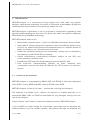
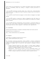
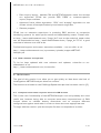
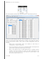
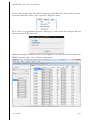
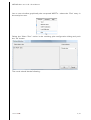
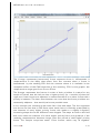
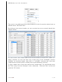
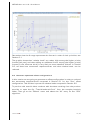
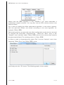
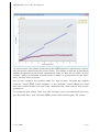
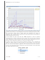
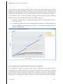
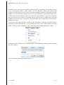
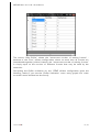
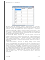
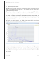
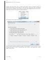
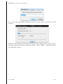
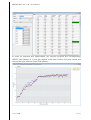
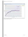
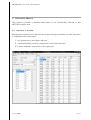
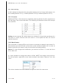
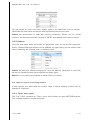
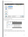
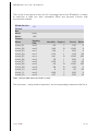
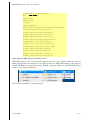
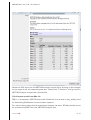
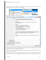
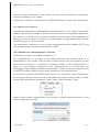
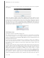
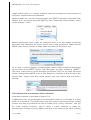
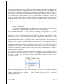
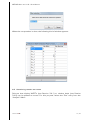
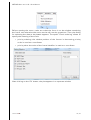
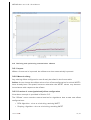
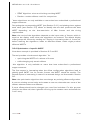
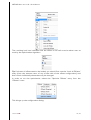
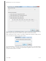
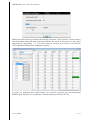
NETCAR-Analyzer V1.6.1 User Manual
Author : Jörn Migge
Verifier : Nicolas Navet, Lionel Havet
Version: DRAFT
Date : 21/2/2011
Contents
1 Introduction..............................................................................................................................................................3
1.1 Licence of the software..............................................................................................................................3
1.2 Installation............................................................................................................................................................4
1.3 Support...................................................................................................................................................................4
1.4 New releases and updates ......................................................................................................................5
2 Quick-start.................................................................................................................................................................5
2.1 Compute worst-case response times of CAN frames...........................................................5
2.2 Compute load indicators.........................................................................................................................10
2.3 Generate optimized offset configurations..................................................................................12
2.4 Compute worst-case transmission buffer occupations....................................................16
2.5 Optimize specific offsets.........................................................................................................................20
2.6 Incremental design.....................................................................................................................................25
3 Reference Manual............................................................................................................................................30
3.1 Overview of the GUI.....................................................................................................................................30
3.2 Data editing......................................................................................................................................................31
3.2.1 Creation..........................................................................................................................................................31
3.2.2 Modification.................................................................................................................................................31
3.2.3 Deletion..........................................................................................................................................................32
3.3 Open or import of existing models...................................................................................................32
3.3.1 “Open” menu entry..................................................................................................................................32
3.3.2 “Recent files” menu entry..................................................................................................................33
3.3.3 Import model from Csv file...............................................................................................................33
3.3.4 Import model from Dbc file..............................................................................................................36
3.4 Worst-case analysis...................................................................................................................................38
3.4.1 Worst-case response-times of frames....................................................................................38
3.4.2 Relative loads.............................................................................................................................................39
3.4.3 Worst-case transmission buffer utilization..........................................................................41
3.5 Visualizing results as curves................................................................................................................43
3.6 Defining and optimizing transmission offsets..........................................................................44
3.6.1 Import..............................................................................................................................................................44
3.6.2 Manual editing...........................................................................................................................................44
3.6.3 Creation of a new (optimized) offset configuration.........................................................44
3.6.4 Optimization of specific WCRT.......................................................................................................45
©2011 RTaW
1/49
NETCAR-A NALYZER V1.6.1 U SER M ANUAL
3.7 Exporting data................................................................................................................................................49
3.7.1 Copy/Paste.................................................................................................................................................49
3.7.2 Import into RTaW-Sim.........................................................................................................................49
4 References............................................................................................................................................................49
©2011 RTaW
2/49
NETCAR-A NALYZER V1.6.1 U SER M ANUAL
1
Introduction
NETCAR-Analyzer is a worst-case timing analysis tool that helps the system
designer optimize the scheduling of frames on Controller Area Network (CAN) and
check that the requirements on transmission delays are met.
NETCAR-Analyzer implements a set of proprietary configuration algorithms that
typically enable doubling the bus load [1], which may defer the need for additional
CAN networks and FlexRay technology.
NETCAR-Analyzer feature list:
• Worst-case response times / jitters on CAN with and without frame offsets
• Near-optimal offsets assignment algorithms with user-defined performance
criteria: e.g. optimize the worst-case response times for a specific subset of
tasks, for instance, the 10 lowest priority frames
• Exhibit the situations leading to the worst-case: results can be checked by
simulation (e.g. with RTaW-Sim) or testing
• Enable dimensioning transmission/reception buffers at the ECU and
communication controller level
• Handle both FIFO and prioritized waiting queues at the ECU level
• Fast multi-core implementation: typically, an exact response time
computation requires less than 30 seconds for 100 frames on a dual-core
system
1.1 Licence of the software
NETCAR-Analyzer is copyrighted by INRIA, INPL and RTaW. It has been developed
since 2005, first by INRIA and INPL, then by RTaW since 2008
NETCAR-Analyzer is free for all uses – commercial, training and research.
The software is provided “as-is”, without any express or implied warranty. In no
event shall INRIA, INPL or RTaW be held liable for any damages arising from the
use of the software.
In this Licence, "the Product" means the software product "NETCAR-Analyzer".
- You may NOT not resell, charge for, sub-license, rent, lease, loan or distribute the
Product without our prior written consent. We reserve the right to withdraw any
©2011 RTaW
3/49
NETCAR-A NALYZER V1.6.1 U SER M ANUAL
such consent (or part thereof) for any reason and without notice and to demand
that you immediately cease any activity in respect of which permission is
withdrawn.
- You may NOT repackage, translate, adapt, vary, modify, alter, create derivative
works based upon, or integrate any other computer programs with, the Product in
whole or in part.
- You may NOT use the Product to engage in or allow others to engage in any illegal
activity.
- You may NOT transfer or assign your rights or obligations under this Licence to
any person or authorise all or any part of the Product to be copied on to another
user's computer.
- You may NOT decompile, disassemble, reverse engineer or otherwise attempt to
discover the source code of the Product except to the extent that you may be
expressly permitted to reverse engineer or decompile under applicable law.
1.2 Installation
Installer based distribution is available for Windows. More information and the
download links are available at url :
http://www.realtimeatwork.com/downloads/
1.3 Support
Free support is available through the forum at url :
http://www.realtimeatwork.com/forum/.
For companies requiring guaranteed results, RTaW is offering professional
support, customized developments, training and R&D services and is committed to
providing the highest level of services for the products it develops. Services
include:
• Priority Technical Support by email, phone or remote control software.
RTaW’s technical support will respond within 1 or at most 2 business days.
Support is available in English, French, German or Italian.
• Maintenance : RTaW will do its best to correct reproducible issues in its
software as soon as possible and provide workaround solutions. Besides,
RTaW is ready to implement and maintain customer-specific versions.
©2011 RTaW
4/49
NETCAR-A NALYZER V1.6.1 U SER M ANUAL
•
•
•
Data import/export : besides CSV and NETCAR-Analyzer native format that
are supported, RTaW can provide DBC, FIBEX or customer-specific
import/export utilities.
Advanced frame offset algorithms: “SOA” and “shaping” algorithms to set
offsets values, offset optimization by local-search algorithm.
Gateway support.
RTaW has an extensive experience in providing R&D services to companies
developing systems for which performance and dependability matter. Please refer
to http://www.realtimeatwork.com/?page_id=5 and to the technical papers that
can be downloaded at http://www.realtimeatwork.com/?page_id=75 for a good
overview of what we are used to do.
Professional support and custom extensions available – see our offer at url:
http://www.realtimeatwork.com/wp-content/uploads/support-NETCARAnalyzer.pdf
1.4 New releases and updates
To be be kept updated with new releases and updates, subscribe to our
eNewsletter at url :
http://www.realtimeatwork.com/#subscribe
2
Quick-start
The goal of this section is to allow you to get quickly an idea about the kind of
investigations NETCAR-Analyzer allows to conduct.
The tutorials are based on the CAN High-Speed example that has been used in [3].
2.1 Compute worst- case response times of CAN frames
This is the main functionality of the NETCAR-Analyzer tool and probably the most
useful one, because being able to compute worst-case response-times of CAN
frames allows to validate latency constraints and to compare different
configurations against each other in order to chose the most appropriate one.
To begin with the tutorial, open the sample file that corresponds to its start:
©2011 RTaW
5/49
NETCAR-A NALYZER V1.6.1 U SER M ANUAL
Go to the samples/tutorials folder and chose the file “Tutorial-landmark-0.xml”.
As can be noticed, besides the basic frame properties like the identifier or the
period, one transmission offset configuration is defined that assigns the offset 0
to every frame (column “Offset : Zero”). Such an offset configuration means the
following :
•
When frame communication starts, one instance of each frame is
instantiated (= ready for being sent).
•
The second instance of each frame is instantiated after a time equal to its
period, which is generally not the same for all frames.
•
After a time equal to the so called hyper-period (= smallest common
multiple of all frame periods), all frames are again instantiated at the
same time. This kind of situation is also known as “critical instant” in the
worst-case analysis literature [1].
©2011 RTaW
6/49
NETCAR-A NALYZER V1.6.1 U SER M ANUAL
Let us now compute the worst-case response-time (WCRT) of the frames. For this
purpose, select the “Wcrt” entry from the “Analysis” menu :
As a result, a progress-bar appears, although in most cases the analysis will not
take more than a few seconds :
When the analysis is done, a new column appears : for each frame it contains the
WCRT induced by the “Zero” offset configuration.
©2011 RTaW
7/49
NETCAR-A NALYZER V1.6.1 U SER M ANUAL
Let us now visualize graphically the computed WCRTs : select the “Plot” entry in
the analysis menu.
Select the “Wcrt: Zero” series in the resulting plot configuration dialog and push
the “Ok” button.
The result should be the following :
©2011 RTaW
8/49
NETCAR-A NALYZER V1.6.1 U SER M ANUAL
The Y-range represents (worst-case) frame response times in milliseconds. A
response-time is the delay that spans from the moment when a frame is
instantiated by the sending ECU and the moment where it is available in the
reception buffers of the CAN controller of the receiving ECU. In this graphic, the
response-time range goes from 0ms to 30ms.
The X-range represents the frames in order of their priorities. It means for any
couple of frames that the left one has a higher priority (i.e. a smaller id) than the
right one. If two frames are adjacent, it means that there is no other frame with a
priority in between. The later does however not mean that the frame priorities are
necessarily adjacent – that would just be one possible case.
In our example, the resulting graph looks like a line with steps. The line segments
are due to the fact that in the worst case, each frame is basically preempted by
one instance of every higher priority frame; this leads to a slightly irregularly
increasing shape due to the different frame lengths. The steps are due to the fact
that more than one instance of a same higher priority frame may preempt, if the
resulting response-time becomes longer than the period of that higher priority
frame. The sample comprises seven 10ms frames, which may all together
©2011 RTaW
9/49
NETCAR-A NALYZER V1.6.1 U SER M ANUAL
preempt twice, as soon as the worst-case response-time become longer than
10ms; this happens to “frame80” for example.
When the response-time is longer than 20ms, then three instances of the 10ms
frames and two instances of the 20ms frame may preempt, which leads to an even
larger step.
2.2 Compute load ind icators
A commonly used indicator for the bandwidth usage of a CAN bus is the periodic
load induced by a set of frames. A periodic load of 50%, for example, means that
half of the bandwidth is used. The other way round, it means that 50% of the
bandwidth should be available for additional frames. In the automotive industry
however, a periodic load of 50% is considered to be already too high 1 ; additional
frames would surely be transmitted over an additional bus. This apparent
contradiction is due to the fact that frames must not just be transmitted but also
within some bounded time. The periodic load does however not take into account
these constraints and is thus of limited use, when an engineer wants to express
how much transmission resource is already used or still free.
Let us suppose that the periods of the frames are also the deadlines for their
transmission. Since the worst-case response-times must be smaller than their
deadlines for the constraints to be met, it would be interesting to compare these
with each other. For this purpose, NETCAR-Analyzer provides the possibility to
compute the “relative load” for a frame which is defined to be a fraction expressed
in percent, with the worst-case response-time as numerator, and the
corresponding period (i.e. the deadline to meet) as denominator. A relative load
value above 100%, means that the deadline is missed - in the worst-case. A
relative load value of 50% means that the deadline is largely met (even in the
worst-case), but not only. It also means that it is very likely that more (higher
priority) frames may be added without causing any deadline to be missed, because
the WCRT is equal to the half of the period (i.e. the deadline to meet). Since
relative loads are defined by frame, it is useful to consider the maximum, average,
etc. and to plot them as a curve.
In order to compute and visualize the relative loads for our example, just continue
with the resulting data set from the tutorial in Section 2.1 or open the
corresponding file called “Tutorial-landmark-1.xml”.
Select the “Load Indicator” entry from the “Analysis” menu :
It is one of the major interest of verification tools, such as NETCAR-Analyzer, to help the designer maximize the use of
hardware resources. With typical applicative-level timing constraints, in our experience, 60% of bus load can be
achieved if the network is well configured, which in the first place involves using a tool like NETCAR-Analyzer (see ref
“pushing the limits”).
1
©2011 RTaW
10/49
NETCAR-A NALYZER V1.6.1 U SER M ANUAL
The result is an additional column that contains for each frame the relative load, as
defined above: “Rel-Load: Zero”.
By clicking on the column header, you can sort the lines so as to easily identify the
highest values.
As can be seen, the relative load of one of the frames is around 75%, which is a
better indicator for the fact that only a little part of the bandwidth remains
available at priorities higher than that of “frame62”, because the wort-case
response-time of that frame is already close to the deadline (=period).
To get a better idea of how the relative load “bottle-necks” are distributed chose
the “Plot” entry from the “Analysis” menu, select the “Rel-Load: Zero” series and
push the “Ok” button :
©2011 RTaW
11/49
NETCAR-A NALYZER V1.6.1 U SER M ANUAL
Remember that the X-range represents the frames in order of their priorities, see
Section 2.1.
The graphic shows that “relative loads” are rather high among the higher
frames (left part) and that adding an additional frame among the higher
frames (in the left-most third) is very likely to cause deadline failures. In
2.3, we show how worst-case response-times, and thus relative loads,
reduced.
priority
priority
Section
can be
2.3 Generate optimized offset configurations
In this section we are going to generate an offset configuration in order to reduced
the worst-case response-times computed in Section 2.1 for the “Zero” offset
configuration. This will also improve the relative loads computed in Section 2.2.
To perform this tutorial either continue with the data resulting from the previous
tutorials or open the file “Tutorial-landmark-2.xml” from the samples/tutorials
folder. Then go to the “Offsets” menu and select the “All” entry for the “SOA”
algorithm :
©2011 RTaW
12/49
NETCAR-A NALYZER V1.6.1 U SER M ANUAL
Notice that the SOA algorithm is only available if you have subscribed a
professional support contract. You may also use the DOA, which produces less
optimal offsets.
As a result of invoking the offset optimization algorithm, a new column appears,
with the optimized offsets and named according to the used algorithm, for
example: “Offset: SOA”.
Before being able to compare this new offset configuration to the old one, we need
to compute the worst-case response-times : chose the “Wcrt” entry in the
“Analysis” menu and then select “Offset: SOA” (name of the column that contains
the generated offsets). The resulting column is “Wcrt: SOA”.
In order to make a comparative plot, select “Plot” from the “Analysis” menu, then
check the “Offset: Zero” and “Offset: SOA” series
and finally push the “Ok” button. The following graphic is then shown :
©2011 RTaW
13/49
NETCAR-A NALYZER V1.6.1 U SER M ANUAL
As can be seen, the offsets produced by the SOA algorithm significantly reduces
the worst-case response-times of the frames. The reason is that the transmission
offsets do spread out the frame instantiation times, so that the so called “critical
instant”, where an instance of each frame is ready for transmission at the same
time, can not occur anymore.
Let us also compare the relative loads. For this purpose, compute the relative
loads for “Wcrt: SOA” (“Load indicator” in the “Analysis” menu). Make sure that
the frame table window has the focus, otherwise the menu entries will remain
grayed out.
To create the plot, select “Plot” from the “Analysis” menu and check this time only
the “Rel-Load: Zero” and “Rel-Load: SOA” series, before pushing the “Ok” button :
©2011 RTaW
14/49
NETCAR-A NALYZER V1.6.1 U SER M ANUAL
The graphic shows that the relative loads are now all below 40%. Notice that the
periodic load of the bus is not changed by transmission offsets (still equal to 50%).
But transmission offsets allow to better exploit the bandwidth with respect to
deadlines : with a relative load of under 40% for all frames, there is more slack for
additional (high priority) frames.
In this section we have seen that the “SOA” algorithm is able to produce
instantaneously an offset configuration that induces very low worst-case response
times. Note that is mainly due to the fact that the frames have (quasi) harmonic
periods: shorter periods are dividers of many of the longer periods.
In order to get an idea of how good the algorithm performs, let us compute the
WCRT for random offsets. For this purpose, go to the “Offsets” menu and select
the “All” entry for the “Random” algorithm and compute the worst-case responsetimes for the generated offsets. Furthermore, go to the “Analysis” menu and select
the “Wcrt Lower Bound” entry.
©2011 RTaW
15/49
NETCAR-A NALYZER V1.6.1 U SER M ANUAL
This computes lower bounds, below which worst-case response-times can not be
pushed by any offset algorithm. It does not mean that this lower bound can be
reached by any algorithm, but when worst-case response-times are already close
to that lower bound, then it is not worth trying to improve the offsets any further.
A comparative plot of the worst-case response-times induced by the different
offsets and the lower bound, shows that the “SOA” algorithm
1. produces offsets that are significantly better than random offsets and are
thus worth using
2. produces very good worst-case response-times that are probably difficult to
improve globally; the optimization of specific worst-case response-times is
shown in Section 2.5.
2.4 Compute worst- case transmission buffer occupations
The worst-case number of frames that may be waiting at the same time for
transmission in a CAN controller is a useful information when choosing a strategy
to avoid the so called “inner priority inversion”, see [4]. An “inner priority inversion”
occurs, when a frame instance is ready for transmission and has a priority higher
then that of all instances (of other frames) currently in the transmission buffer(s),
©2011 RTaW
16/49
NETCAR-A NALYZER V1.6.1 U SER M ANUAL
but the former can not participate in the arbitration because it is not (yet) located
in a transmission buffer, since these are all occupied. When the worst-case
number of waiting frames is known, a simple strategy consists in allocating enough
buffers for transmission, so that even in the worst-case all frames can be stored in
a free transmission buffer an thus no “inner priority inversion” may occur. Notices
that the worst-case number of waiting frames can be much smaller than the total
number of frames that a controller can potentially send, especially if transmission
offsets are used.
To perform this tutorial either continue with the data resulting from the previous
tutorials or open the data set “Tutorial-landmark-3.xml” from the samples/tutorials
folder. Then go to the “Analysis” menu and select the “Buffer Utilization” entry :
and choose the “Offset: Zero” configuration in the resulting dialog, before pushing
the “Ok” button :
As a result the following window appears :
©2011 RTaW
17/49
NETCAR-A NALYZER V1.6.1 U SER M ANUAL
The column “Max Buffer” shows the “worst-case number of waiting frames” :
because of the “Zero” offsets configuration, where at some time all frames are
instantiated together (critical instant), the “worst-case number of waiting frames”
is simply equal to the number of different frames that may be send by the
controller.
Computing the Buffer utilization for the “SOA” offsets configuration gives the
following result (if you see the “Buffer Utilization” menu entry grayed out, make
sure the frames window has the focus):
©2011 RTaW
18/49
NETCAR-A NALYZER V1.6.1 U SER M ANUAL
As can be seen, the “worst-case number of waiting frames” are much lower,
thanks to the transmission offsets that spread-out the frame instantiation times. It
means for example, that with the “DOA” offsets configuration, 4 transmission
buffers would be enough on “ECU_1” for avoiding “inner priority inversion” : when
ever a frame is instantiated, at least one transmission buffer is free to stored it.
This strategy is quite simple to implement compared to other more sophisticated
ones like the use of transmission cancellation.
The column “Max Backlog” represents the “worst-case number of frames, still
present in the transmission buffer(s) when the periodic COM task starts to look
again for frames to instantiate”. Here we suppose that the period of the COM task
is the greatest common divider of the offsets and periods – in other words, the
largest period that allows to implement the transmission offsets with the help of a
periodic task.
If that maximal backlog is zero, then the following strategy for inner priority
inversion avoidance may be used : if the periodic COM task instantiates frames in
the order of their priority, then theoretically, only one transmission buffer (and a
software queue) would be enough to avoid inversion, because new frames would
only be instantiated when all pending frames have already been transmitted. Notice
that probably more than one transmission buffer would be needed to avoid the so
called “external priority inversions”, see [4]. These kind of inversions occur, when a
controller has frames to send but is not fast enough to refill the transmission
buffer and thus a frame may miss an arbitration in which it should have
participated.
©2011 RTaW
19/49
NETCAR-A NALYZER V1.6.1 U SER M ANUAL
2.5 Optim ize specific offsets
NETCAR-Analyzer provides algorithms for optimizing offsets according to WCRT
based criteria. Notice that this algorithm is only available if you have subscribed a
professional support contract.
The goal is to modify an existing offset-configuration such that the WCRTs of all or
a subset of frames become smaller or remain the same. The WCRT of the frames
that do not belong to the subset may increase.
This allows for instance, to reduce the relative load of (certain) frames as we will
see in this section. To perform this tutorial either continue with the data resulting
from the previous tutorials or open the file “Tutorial-landmark-3.xml” from the
samples/tutorials folder.
Remember the relative loads for the “SOA” offsets based WCRTs (see Section
2.2). The plot of these relative loads looks like this :
In the above screen-shot we have located the mouse pointer over the highest point
in order to identify the corresponding frame. According to the x-coordinate, it is
the frame with id=183 (decimal format). If we sort the frame table according to
the “FrameId” column, we can easily find the corresponding frame name:
“frame12”. The second highest relative load is that of the frame called “frame62”,
with id=193.
©2011 RTaW
20/49
NETCAR-A NALYZER V1.6.1 U SER M ANUAL
Imagine that we would like to reduce the relative loads for these frames, by
changing the offsets appropriately. For this purpose, select the “Optimize Offsets”
entry from the “Offsets” menu (make sure the frame table window has the focus,
otherwise the menu entries will remain grayed-out):
This brings up the configuration dialog :
Select “Search criterion based on custom frames WCRT”, mark “frame12” in tab
3, mark “frame62” in tab 1 and push the “Ok” button. Then select the “Offset:
SOA” configuration :
©2011 RTaW
21/49
NETCAR-A NALYZER V1.6.1 U SER M ANUAL
As a result, the optimization algorithm starts its work, which may take 10 to 20
minutes :
When the optimization process has finished, push the “Done” button. A new column
has been generated with the optimized offsets: “Offset: SOA/1”. Modified offsets
are displayed in green:
©2011 RTaW
22/49
NETCAR-A NALYZER V1.6.1 U SER M ANUAL
In order to evaluate this optimization, you should compute the corresponding
WCRTs (see Section 2.1) and the relative loads (see Section 2.2) and create the
comparison plot with the initial DOA offsets :
©2011 RTaW
23/49
NETCAR-A NALYZER V1.6.1 U SER M ANUAL
The comparison of the WCRT graphs shows that the WCRT of some lower priority
frames, including “frame12” and “frame62” have decreased - at the cost of
increasing the WCRTs of other frames, which are mainly lower priority ones.
2.6 Incremental design
When a new version of a product is created, it frequently happens that as much as
possible of an existing product should be reused. For a frame set, this means that
new signals need to be added to existing frames or that new frames have to be
added for new signals, while leaving all other configuration parameters (period, id, ,
signal to frame allocation, etc) unchanged. For the transmission offsets, this
means that good values need to be found for the new frames while keeping the
offsets of the existing frames. The optimization algorithms provided by NETCARAnalyzer are the solution to this problem.
To be able to add new frames you must first make sure that no worst-case
response-times or other computed columns are contained in the NETCAR-Analyzer
file. You can for example make a copy of the file from previous tutorial steps and
delete all computed columns (see Section 3.2.3 for more details).
You may also simply open the file “Tutorial-landmark-5.xml”, which contains four
additional frames, with zero offsets and induced worst-case response-times. T his
file has been created as follows: open the file “Tutorial-landmark-0.xml” from the
©2011 RTaW
24/49
NETCAR-A NALYZER V1.6.1 U SER M ANUAL
samples/tutorials folder (see Section 2.1) as basis and regenerate the “SOA”
offset configuration (see Section 2.3). Once the “Offset: SOA” column is created
we suggest to delete the “Offset: Zero” column because we do not need it any
more (right-click on the column header to bring up the menu with the “Delete”
entry).
Now we need to lock the existing offsets, so that the optimization algorithm does
not change them. For this purpose right-click into a cell of the “Offset: SOA”
column and select the “Lock All Offsets” entry.
Now we are ready to add the following new frames:
Frame name
Sending ECU
Id
Period
Payload
FrameNew1
Ecu_0
100
40
7
FrameNew2
Ecu_4
170
100
6
FrameNew3
Ecu_9
300
50
5
FrameNew4
Ecu_8
470
200
8
Go to the last line in the frame table and enter the properties of the frames
in order to obtain the following:
©2011 RTaW
25/49
NETCAR-A NALYZER V1.6.1 U SER M ANUAL
Leave the offsets of the new frames to 0.
In order to get an idea of the worst impact of adding these new frames, compute
the worst-case response-times and plot them:
As can be seen, adding the four new frames with zero offset make the worst-case
response-time of some lower priority frame increase around 8ms.
Now let us see if we can improve the situation by optimizing the offsets of the new
frames. For this purpose select the “Optimize” entry in the “Offset” menu.
Remember that this algorithm is only available if you have subscribed a
professional support contract.
©2011 RTaW
26/49
NETCAR-A NALYZER V1.6.1 U SER M ANUAL
Keep the “Search criterion based on all frame WCRT” selected and click “Start”.
After the initialization phase, the progress-bar starts to move:
When the optimization has finished, click the “Done” button. Then, compute the
worst-case response-times and make a comparison plot:
©2011 RTaW
27/49
NETCAR-A NALYZER V1.6.1 U SER M ANUAL
As can be seen, after optimization of the offsets of the new frames, all worst-case
response-times are below 5ms.
©2011 RTaW
28/49
NETCAR-A NALYZER V1.6.1 U SER M ANUAL
3
Reference Manual
This section provides a detailed description of all functionality offered by the
NETCAR-Analyzer tool.
3.1 Overview of the GUI
Besides the classical menu bar at the top (see the figure below), the user interface
is subdivided into three parts:
1. bus properties in the upper left part
2. connected ECUs and their properties in the lower left part
3. frames and their properties in the right part
©2011 RTaW
29/49
NETCAR-A NALYZER V1.6.1 U SER M ANUAL
3.2 Data editing
In this section we describe how new data entities such as buses and frames, can
be created (Section 3.2.1), modified (Section 3.2.2) or deleted (Section 3.2.3).
3.2.1 Creation
Additional ECUs or frames can be created by entering values for their properties in
the last line of the concerned table. The following screen-shot shows the example
of a new ECU:
Advise: do not save the file, while values are missing for some of the attributes of a
new ECU or frame, because this will result in a corrupted file that can not be
opened anymore.
3.2.2 Modification
The properties of existing ECUs and frames can directly be edited in the tables. For
this purpose you need to click a first time on the concerned table cell, in order to
select it and then you need to click a second time to enable editing.
Notice: For the changes do be effective, you need to hit “Enter” or move the focus
to an other cell.
It is also possible to change the titles of offset, WCRT and relative load columns.
For this purpose, right-click on the column header and select “Rename” from the
menu.
The column header becomes editable and you can enter the new name :
©2011 RTaW
30/49
NETCAR-A NALYZER V1.6.1 U SER M ANUAL
Do not forget to push the enter button before you leave the column header,
otherwise the new name will be lost and replaced by the previous one.
Advice: we recommend to keep the naming convention “Offset: xyz” for offset
columns, so that the automatic naming of WCRT and relative load columns works.
3.2.3 Deletion
Columns that have been computed or generated such as worst-case responsetimes, relative-loads and offsets can be deleted, by right-clicking on the column title
and by selecting the “Delete” entry in context menu:
Advice: At least one offset configuration must be defined, otherwise a saved file
will be corrupted and can not be opened correctly again.
Notice: It is currently not possible to delete ECUs or frames.
3.3 Open or import of existing models
In this section are described the various ways in which existing models can be
opened or imported.
3.3.1 “Open” menu entry
The “File” menu contains an “Open” entry which allows to open NETCAR-Analyzer
files located anywhere on the computer:
©2011 RTaW
31/49
NETCAR-A NALYZER V1.6.1 U SER M ANUAL
3.3.2 “Recent files” menu entry
The “File” menu contains a “Recent Files” entry which provides an easy access to
recently opened files:
3.3.3 Import model from Csv file
As its name says, this kind of file contains “Character Separated Values” (CSV) but
it is easier to understand as textual data under a tabular form, as shown in Table
1.
©2011 RTaW
32/49
NETCAR-A NALYZER V1.6.1 U SER M ANUAL
The format is the same as the one for importing frames into RTaW-Sim. It allows
to describe a CAN bus with connected ECUs and periodic Frames with
transmission offsets:
RTaW-Sim-CsvFormat
Bus
Name
Speed
Frames
Name
frame_01
frame_02
frame_03
frame_04
frame_05
frame_06
frame_07
frame_08
frame_09
frame_10
frame_11
frame_12
1.0
body
125
Sending
ECU
ecu0
ecu0
ecu1
ecu1
ecu1
ecu2
ecu2
ecu2
ecu3
ecu3
ecu3
ecu3
Identifier Payload
23
345
122
212
341
78
976
52
36
6
222
107
7
8
1
1
8
1
1
8
8
8
7
2
Period
Offset
100
1000
200
100
1000
200
100
1000
100
50
200
500
0
0
0
50
120
0
50
120
0
35
0
70
Table 1: Sample CSV import file shown as table
The character ';' being used as separator, the corresponding contents of the file is:
©2011 RTaW
33/49
NETCAR-A NALYZER V1.6.1 U SER M ANUAL
RtaW-Sim -Csv -Format;1.0
Bus
Name;body
Speed;125
Frames
Name;Sending
ECU;Identifier;Payload;Period;Offset
frame_01;ecu0;23;7;100;0
frame_02;ecu0;345;8;1000;0
frame_03;ecu1;122;1;200;0
frame_04;ecu1;212;1;100;50
frame_05;ecu1;341;8;1000;120
frame_06;ecu2;78;1;200;0
frame_07;ecu2;976;1;100;50
frame_08;ecu2;52;8;1000;120
frame_09;ecu3;36;8;100;0
frame_10;ecu3;6;8;50;35
frame_11;ecu3;222;7;200;0
frame_12;ecu3;107;2;500;70
Table 2: Sample CSV import file shown as text
NETCAR-Analyzer can not directly import the file. You rather need to use an
external tool able to transform the CSV file into an NETCAR-Analyzer. This tool is
called “Csv2Nca” and located in the “RTaW” program folder, in the Windows Start
menu - if you have installed it:
The GUI of “Csv2Nca” is the following:
©2011 RTaW
34/49
NETCAR-A NALYZER V1.6.1 U SER M ANUAL
Select the CSV input file and NETCAR-Analyzer output file by clicking on the triangle
on the right of the corresponding text box. Finally click “Transform” and go back to
NETCAR-Analyzer to open the imported file.
3.3.4 Import model from Dbc file
DBC is a proprietary VECTOR Informatik Gmbh file format that is very widely used
for describing CAN based communication systems.
For users having subscribed a professional support contract, RTaW provides a tool
for transforming DBC files into NETCAR-Analyzer files.
©2011 RTaW
35/49
NETCAR-A NALYZER V1.6.1 U SER M ANUAL
This tool is called “Dbc2Nca” and located in the “RTaW” program folder, in the
Windows Start menu - if you have installed it:
The GUI of “Dbc2Nca” is the following:
Select the Dbc input file and NETCAR-Analyzer output file by clicking on the triangle
on the right of the corresponding text box.
Then you need to provide the bus speed because because the DBC file does not
contain this information.
Furthermore, there are no standard attribute names for frame periods and frame
transmission offsets. The dialog proposes by default the custom attribute names
©2011 RTaW
36/49
NETCAR-A NALYZER V1.6.1 U SER M ANUAL
that are used by the Vector Tool Chain. You can edit the fields and change the
names according to your needs.
Finally click “Transform” and go back to NETCAR-Analyzer to open the imported file.
3.4 Worst-case analysis
The analysis algorithms implemented in the tool perform a so called “worst-case”
analysis: given the properties of the bus and the frames, the algorithms determine
the scenario in which some quantity reaches its worst value. The knowledge of
these worst values allows to check if a certain system configuration allows correct
functioning even in the worst case.
The quantities of interest here, are frame response-times (see Section 3.4.1) and
transmission buffer utilization (see Section 3.4.3).
3.4.1 Worst-case response-times of frames
A hands-on example is provided in Section 2.1.
The response-time of a frame is the delay between the moment when it is
instantiated in the sender ECU and the moment where the transmission of the
frame ends and thus it is available in reception buffers of the receiving ECUs. If
there is a hard latency constraint on the response-times of a frame, then the
knowledge of the longest possible response-time, called worst-case response time
or WCRT for short, allows to verify if the constraint can always be met.
To be able to compute the WCRT of the frames, the frame set must be present in
the tool (see Sections 3.2 and 3.3 on the different ways to achieve this). In order
to start the computation, select the “Wcrt” entry of the “Analysis” menu:
When several offset configurations are present, a dialog opens and asks for the
offset configuration to use:
©2011 RTaW
37/49
NETCAR-A NALYZER V1.6.1 U SER M ANUAL
When the “Ok” button has been pushed, the computation starts and a progressbar appears:
When the analysis is done, a new column appears in the frame table: for each
frame it contains the WCRT induced by the selected offset configuration. The name
of that column is by default based on the name of the offset configuration and has
the prefix “Wcrt:”. The name of the column can be changed, see Section 3.2.2. In
any case, the name of the corresponding offset configuration can always be
visualized in the tool-tip of the WCRT column title (simply move the mouse pointer
over the column title and wait a second):
3.4.2 Relative loads
A hands-on example is provided in Section 2.2.
The relative load of a frame is the WCRT of that frame, expressed as percentage
of the frames deadline, i.e. the longest allowed response-time. Currently, the
period is considered to be the deadline and thus the frames response-times must
be shorter then the period.
If a frame has for example a period (and thus a deadline) of 100ms and a WCRT of
33ms, then the relative load is 33%. A relative load of 33% means first of all that
the deadline is meet. In general, as long as the relative load is below 100%, the
deadline is met.
A relative load of 33% also means that there is 66% slack time left. This slack time
could be used to add more higher priority frames. How much and what kind of
higher priority frames can be added without causing deadline overrun must be
determined through the computation of WCRTs, but a slack of 66% is a good
synthetic indicator of the fact that there is indeed room left for adding frames.
Such a synthetic indicator is useful for monitoring, at project management level,
the evolution of resource usage, because it hides the details such as the exact
values of the deadlines and shows only an essential information about the resource
©2011 RTaW
38/49
NETCAR-A NALYZER V1.6.1 U SER M ANUAL
usage. Notice that it is a better indicator than the average bus load, because it
compares response-times to deadlines.
Relative loads can only be computed after the WCRT have been computed (see
Section 3.4.1 on how to compute WCRTs). Then, select the “Load Indicator” entry
of the “Analysis” menu:
Before opening the menu, make sure that the focus is on the window containing
the frame set, otherwise the menu entries will remain grayed-out. When several
WCRT columns are present, a dialog opens and asks for the one to use:
As a result, a column appears containing the relative loads and with a title based
on the name of the WCRT column, with “Rel-Load:” as prefix, instead of “WCRT:”.
The name of the column can be changed, see Section 3.2.2. In any case, the name
of the corresponding WCRT column can always be visualized in the tool-tip of the
column title: simply move the mouse pointer over the column title and wait a
second:
3.4.3 Worst-case transmission buffer utilization
A hands-on example is provided in Section 2.4.
A CAN frame can only participate in the arbitration phase if it is located in a send
buffer of a controller. The send buffers may be a scarce resource but their limited
number can lead to problems like the so called “inner priority inversion”, see [4].
An “inner priority inversion” occurs, when a frame instance is ready for
transmission and has a priority higher then that of all instances (of other frames)
©2011 RTaW
39/49
NETCAR-A NALYZER V1.6.1 U SER M ANUAL
currently in the transmission buffer(s), but the former can not participate in the
arbitration because it is not (yet) located in a transmission buffer, since these are
all occupied. A simple, but costly and not always realizable solution consists in
having as much send buffers as different frames send by the ECU. But the number
of simultaneously waiting frames can be much smaller, especially if offsets are
used for sending the frames. Knowing the worst-case number of simultaneously
waiting frames would allow to choose exactly the needed number of send buffers
and to perform this way an efficient and safe design choice.
NETCAR-Analyzer does exactly allow this, by computing for each ECU
•
an efficient upper bound on the highest number of simultaneously waiting
frames : “Max Buffer”
•
an efficient upper bound on the highest number of frames still in the send
buffer(s) when the COM task adds new frames: “Max Backlog”
If the “Maximal Backlog” is zero, then the following strategy for inner priority
inversion avoidance may be used : if the periodic COM task instantiates frames in
the order of their priorities, when several frales have to be instantiated at a same
notional moment, then theoretically only one transmission buffer (and a FIFO
software queue) would be enough to avoid inversion, because new frames would
only be instantiated when all pending frames have already been transmitted and
because every batch of simultaneously waiting frames is ordered according to
their priorities. Notice that probably more than one transmission buffer would be
needed to avoid the so called “external priority inversions”, see [4]. These kind of
inversions occur, when a controller has frames to send but is not fast enough to
refill the transmission buffer and thus a frame may miss an arbitration in which it
should have participated.
To be able to compute the worst case buffer utilizations, the frame set must be
present in the tool (see Sections 3.2 and 3.3 on the different ways to achieve this).
In order to start the computation, select the “Buffer Utilization” entry of the
“Analysis” menu:
Before opening the menu, make sure that the focus is on the window containing
the frame set, otherwise the menu entries will remain grayed-out. When several
offset configuration are present, a dialog opens up and asks for the offset
configuration to use:
©2011 RTaW
40/49
NETCAR-A NALYZER V1.6.1 U SER M ANUAL
When the computation is done, the following kind of window appears:
3.5 Visualizing results as curve s
Columns that display WCRTs (see Section 3.4.1) or relative loads (see Section
3.4.2) can be plotted as curves. For this purpose, select the “Plot” entry from the
“Analysis” Menu:
©2011 RTaW
41/49
NETCAR-A NALYZER V1.6.1 U SER M ANUAL
Before opening the menu, make sure that the focus is on the window containing
the frame set, otherwise the menu entries will remain grayed-out. Then, the dialog
for selecting the data to be plotted appears. The option “X-axis ordering” allows to
specify the meaning of the x-axis:
•
priority ordering: the relative position of the frames in decreasing priority
order is used as x coordinate
•
priority value: the value of the frame identifier is used as x coordinate
After clicking on the “Ok” button, the plot appears in a separate window:
©2011 RTaW
42/49
NETCAR-A NALYZER V1.6.1 U SER M ANUAL
3.6 Defining and optimizing transmission offsets
3.6.1 Import
When a frame set is imported, the offsets are also automatically imported.
3.6.2 Manual editing
Any existing offset configuration can directly be edited in the frame table.
Advise: do not change the offset values of an offset configuration for which WCETs
have already been computed, because otherwise the WCRT values may become
inconsistent with respect to the offsets.
3.6.3 Creation of a new (optimized) offset configuration
A hands-on example is provided in Section 2.3.
The “Offsets” menu contains several entries for algorithms that create new offset
configurations:
•
DOA Algorithm : aims at minimizing resulting WCET
•
Shaping * Algorithm: aims at minimizing resulting WCET
©2011 RTaW
43/49
NETCAR-A NALYZER V1.6.1 U SER M ANUAL
•
SOA * Algorithm: aims at minimizing resulting WCET
•
Random: random offsets, useful for comparison
these algorithms are only available to users that have subscribed a professional
support contract.
*
Computing the corresponding WCET (see Section 3.4.1) and plotting them against
each other (see Section 3.5) allows to identify the one that produces the best
WCET depending on the characteristics of the frames and the timing
requirements.
Note: the result of the algorithms depends on the input order of frames, which is
equal to the display order when the algorithms are started. The default display
order groups the frames by sending ecu. Sorting in increasing order of frame ids,
before starting the algorithms, leads to different offsets, which might produce
different WCRTs.
3.6.4 Optimization of specific WCRT
A hands-on example is provided in Sections 2.5 and 2.6.
The tool provides a local-search algorithm * for
•
optimizing the WCRTs of a subset of frames
•
while changing only certain offsets
this algorithm is only available to users that have subscribed a professional
support contract.
*
The first aspect is interesting when the offset configuration algorithms lead to
globally good WCRT, but for certain frames, the WCRT should be smaller. The
second aspect is interesting in case of incremental design, as illustrated in Section
2.6.
Note: the optimization algorithm does not change any existing offset configuration.
It uses an existing one as basis and creates a new one, that take over some of the
offsets, whereas others are different.
If some offsets should not be changed, you must first lock them. For this purpose
click into an offset cell, then right-click to bring up the context menu and select the
“Lock” entry.
©2011 RTaW
44/49
NETCAR-A NALYZER V1.6.1 U SER M ANUAL
The resulting lock icon indicates that the offset in the cell must be taken over as
such by the optimization algorithm:
Tip: If almost all offset need to be locked, you should first use the “Lock all Offsets”
entry (from the context menu of any of the cells of the offset configuration) and
then unlock individually those that may be changed.
In order to run the optimization, select the “Optimize Offsets” entry from the
“Offsets” menu:
This brings up the configuration dialog:
©2011 RTaW
45/49
NETCAR-A NALYZER V1.6.1 U SER M ANUAL
The “Local Search Frame Selection” section, allows to specify for which frames the
WCRT shall be decreased. The WCRT of the other frames may increase.
After pushing the “Start” button, the offset configuration selection dialog comes
up, if more then one offset configuration exists:
The selected offset configuration will be used as starting point for the optimization.
When the “Ok” button is pushed, the optimization algorithm starts its work, which
may take several dozen of minutes :
©2011 RTaW
46/49
NETCAR-A NALYZER V1.6.1 U SER M ANUAL
When the optimization process has finished, push the “Done” button. A new column
has been generated with the optimized offsets. Its name is derived from the initial
algorithm by appending “/1”. You may want to rename the column, see Section
3.2.2. Modified offsets are displayed in green:
In order to evaluate this optimization, you should compute the corresponding
WCRTs (see Section 3.4.1) and the relative loads (see Section 3.4.2).
©2011 RTaW
47/49
NETCAR-A NALYZER V1.6.1 U SER M ANUAL
3.7 Exporting data
3.7.1 Copy/Paste
In any table you can select a range of cells and copy the contained data as table to
word processors or spreadsheet tools. In particular, you can easily select an entire
table by clicking on its left upper corner:
3.7.2 Import into RTaW-Sim
You can also import the NETCAR-Analyzer files into RTaW-Sim, in order to
complement the computed WCRT by statistics like the average response times or
by quantiles (the 90% quantile is a threshold that is overrun in 90% of the cases,
in the average).
It also allows to simulate the worst-case scenarios that NETCAR-Analyzer has
identified for each of the computed WCRTs.
More information about RTaW-Sim can be found here:
http://www.realtimeatwork.com/?page_id=1217
4
References
[1] M. Grenier, L. Havet, N. Navet, “Pushing the limits of CAN – Scheduling frames
with offsets provides a major performance boost“, Proc. of the 4th European
Congress Embedded Real Time Software (ERTS 2008), Toulouse, France, January
29 – February 1, 2008.
[2] M. Grenier, J. Goossens, N. Navet, "Near-Optimal Fixed Priority Preemptive
Scheduling of Offset Free Systems", Proc. of the 14th International Conference on
Network and Systems (RTNS'2006), Poitiers, France, May 30-31, 2006
[3] N. Navet, A. Monot, J. Migge, “Frame latency evaluation: when simulation and
analysis alone are not enough”, 8th IEEE International Workshop on Factory
Communication Systems (WFCS2010), Industry Day, May 19, 2010. Available at
url: http://www.realtimeatwork.com/?page_id=75.
[4] “Specification of CAN Interface”, AUTOSAR v4.0, 2009.
©2011 RTaW
48/49
NETCAR-A NALYZER V1.6.1 U SER M ANUAL
[5] N. Navet, Y-Q. Song, F. Simonot, “Worst-Case Deadline Failure Probability in
Real-Time Applications Distributed over CAN (Controller Area Network) ”, Journal of
Systems Architecture, Elsevier Science, vol. 46, n°7, 2000. Available at url:
http://www.realtimeatwork.com/?page_id=75.
[6] R. Davis, A. Burns, R. Bril, J. Lukkien, “Controller Area Network (CAN)
schedulability analysis: Refuted, revisited and revised”, Real-Time Systems, vol. 35,
n°3, 2007.
©2011 RTaW
49/49