Download View/Open - Oregon State University

AN ABSTRACT OF THE THESIS OF
Brian D. Wichner for the degree of Doctor of Philosophy in Physics presented on
June 16, 1998. Title: Conversion of Laser Phase Noise to Amplitude Noise in a
Lummer-Gehrcke Interferometer and in Oxygen Gas.
Abstract Approved:
Redacted for Privacy
In order to observe laser phase noise, this noise must be converted to
amplitude noise, which can be achieved using either an interferometer or an
absorption resonance in an atomic/molecular vapor or gas. When phase noise is
converted to amplitude noise, it is manifested as a heterodyne signal in the
output of an optical square-law detector. Thus, phase noise is measured by
optical
heterodyne
spectroscopy,
or,
equivalently,
laser
phase
noise
spectroscopy.
In recent work on diode laser noise spectroscopy of rubidium and oxygen, the
observed spectroscopic lineshapes were not in total agreement with theoretical
predictions. We have repeated the previous work on the oxygen A-band
transitions, and we now find qualitative agreement with theory.
In addition, we have measured the diode laser noise spectrum of a LummerGehrcke interferometer (LGI), comparing the heterodyne lineshape of a LGI
transmission spectrum with a qualitative theory that we develop in this thesis.
A theory, from other workers, predicts the intensity fluctuations from a
Doppler-broadened, two-level atomic/molecular system driven with a phase-
diffusing laser field. We show that a simplified version of this theory, which
ignores Doppler effects of the system, is a useful approximation to the complete
theory, by comparing computer-generated heterodyne lineshapes of each, for a
rubidium transition. We apply this approximate theory to an oxygen A-band
transition, and compare these results with our experimental measurements.
For the experimental arrangement used in the present work, diode laser noise
spectroscopy may also include effects of selective reflection, which is dealt with
experimentally and theoretically.
Diode laser phase noise has practical importance in optical communications
and atomic clocks.
Conversion of Laser Phase Noise to Amplitude Noise in a Lummer-Gehrcke
Interferometer and in Oxygen Gas.
By
Brian D. Wichner
A THESIS
Submitted to
Oregon State University
in partial fulfillment of
the requirements for the
degree of
Doctor of Philosophy
Presented June 16, 1998
Commencement June, 1999
Doctor of Philosophy thesis of Brian D. Wichner presented June 16, 1998
APPROVED:
Redacted for Privacy
Major Prof
,r
ysics
Redacted for Privacy
Chair of Department of Physics
Redacted for Privacy
I understand that my thesis will become part of the permanent collection of
Oregon State University libraries. My signature below authorizes release of my
thesis to any reader upon request.
Redacted for Privacy
Brian D. Wichner, Author
Table of Contents
Page
1.
2.
Introduction
1
1.1
Introduction and Background
1
1.2
Diode Laser Heterodyne Spectroscopy
2
1.3 Thesis Outline
4
Basic Principles and Theory of Diode Lasers
5
2.1
Introduction to Diode Lasers
2.2 Wavelength Tuning
8
2.3 Diode Laser Models
9
2.4 Optical Feedback
11
2.5 Diode Laser Noise
12
2.5.1
Diode Laser Noise Models
2.5.2 Types of Diode Laser Noise
2.5.3
3.
5
Relaxation Oscillations and the Diode
Laser Power Spectrum
Theory of Diode Laser Phase Noise and its Conversion to
Amplitude Noise
13
14
19
23
3.1
Introduction
23
3.2
Mathematical Description of Phase Modulation
33
3.3 Using a Lummer-Gehrcke Interferometer to
Measure Laser Phase Noise
3.3.1
Motivation
3.3.2 Lummer-Gehrcke Interferometer
37
37
38
Table of Contents (Continued)
Page
3.4 Lummer-Gehrcke Heterodyning
42
3.5 Heterodyning with an Atomic/Molecular Vapor or Gas
43
3.5.1
Introduction
3.5.2 Heterodyne Theory for a Diode Laser Emission
Obeying the Phase-Diffusing Model
4.
46
3.6 Selective Reflection as a Possible Source of Optical
Feedback
51
3.7 (Optional) Heterodyne Detection and the Correlation
Function
54
Experimental Techniques
57
4.1
5.
43
Diode Lasers
57
4.2 Diode Laser Mounting and Temperature ContrOl
59
4.3 Optical Layout Including L GI and the Oxygen Cell
60
4.4 Detector Circuit
66
4.5 Diode Laser Drive Circuit
68
4.6 Computer Control
71
4.7 Spectral Scanning Method
73
4.8 Radio Frequency Spectrum Analyzer
75
Experiment Results
80
5.1
Lummer-Gehrcke Interferometer Heterodyne Spectra
5.1.1
NIR Diode Laser Spectra
5.1.2 Visible Diode Laser Spectra
80
80
85
Table of Contents (Continued)
Page
5.2 Oxygen Heterodyne Spectra
88
5.3 Oxygen Spectra for the case of a Diode Laser with Intentional 103
Fresnel Feedback
6.
5.4 Spectra of Diode Laser with Unintentional Fresnel Feedback
105
Summary and Conclusion
112
Bibliography
116
Append ices
119
List of Figures
Page
Figure
2.1
AIGaAs -type diode laser chip structure
5
2.2
Schematic view of the light output power versus current
characteristics of a diode laser
7
2.3
760 nm diode laser emission spectrum showing primary and
secondary modes.
10
2.4
RIN spectra for a GaAIAs diode laser, driven at 20% above
threshold
15
2.5
Measured RIN of a GaAlAs diode laser versus drive current
17
2.6
Frequency noise spectra for a typical GaAIAs diode laser
18
2.7
Spectral lineshape calculated for a single-mode diode laser
operating at 0.5 mW and 1 mW
22
3.1
Phasor representation of a) amplitude modulation, and b)
frequency modulation.
27
Frequency-domain representation of the rotating vectors in
29
3.2
Figure 3.1
3.3
Carrier and sidebands tuned across an absorption line
31
3.4
Carrier and sidebands for single-tone frequency modulation
35
3.5
Carrier and sidebands for
amplitude modulation
3.6
Lummer-Gehrcke Interferometer
38
3.7
LGI output spectra for several values of exiting beam number,
calculated using equation 3.23.
41
simultaneous
frequency
and
36
List of Figures (Continued)
Page
Figure
3.8
Calculated transmission spectrum of oxygen
45
3.9a
Calculated heterodyne peak height and central minimum
height of Rubidium with and without Doppler integration,
versus spectrum analyzer frequency.
49
3.9b
Calculated heterodyne FWHM and center width of
Rubidium with and without Doppler integration,
versus spectrum analyzer frequency.
50
3.10
Schematic of selective reflection versus detuning
51
3.11
Graphical depiction of directional differences between specular
and selective reflection
52
4.1
Schematic description of experimental apparatus, showing LGI
61
4.2a
Scheme used to monitor, in real-time, the emission spectrum of
the diode laser
61
4.2b
Two examples of monitor output of the apparatus shown in
62
Figure 4.2a. An emission spectrum for a 670 nm and a 760 nm
diode laser is shown in the left and right figure, respectively.
4.3
Oxygen gas cell details
64
4.4
Measured transmission spectrum of LGI.
65
4.5
Photodetector description of apparatus circuit
67
4.6
Drive circuit for diode laser
69
4.7
Half a heterodyne lineshape showing spectral drift when the
measurement process was paused for 500 seconds
76
4.8
Radio frequency spectrum analyzer
77
5.1
LGI heterodyne spectrum of the 760 nm diode laser
81
5.2
Diode laser emission spectra for heterodyne data of Figure 5.1
82
List of Figures (Continued)
Figure
Page
5.3
Apparatus used for measuring diode laser amplitude noise
83
5.4
Amplitude noise spectrum for a 670 nm diode laser, operating
at a power level of 6.6 mW
84
5.5
Heterodyne spectra for a 670 nm diode laser, for two emission
power levels
86
5.6
Diode laser emission spectrum for the case of Figure 5.5
87
5.7
Heterodyne spectrum showing two oxygen transitions, as noted
in the figure
90
5.8
Previously reported heterodyne spectra for oxygen
92
5.9
Comparison of theory and experiment for heterodyne peak
height
95
5.10
Comparison of theory and experiment for heterodyne FWHM
96
5.11
Comparison of theory and experiment for heterodyne center
width
98
5.12
Comparison of theory and experiment for heterodyne central
minimum height
99
5.13
Heterodyne lineshape peak height asymmetry
100
5.14
Apparatus for testing the presence of selective reflection effects
102
5.15
Amplitude noise spectra for two drive current values, of a 760
nm diode laser, subjected to optical feedback
104
5.16
Heterodyne lineshape of 760 nm diode laser with optical
feedback
106
5.17a
Heterodyne lineshapes of oxygen with a relatively small amount
of diode laser optical feedback
109
5.17b
Heterodyne lineshapes of oxygen with an increasing amount of
diode laser optical feedback
109
List of Figures (Continued)
Page
Figure
5.17c
Heterodyne lineshapes of oxygen with slightly more diode laser
optical feedback than in Figure 5.17b
110
5.17d
Heterodyne lineshapes of oxygen with slightly more diode laser
optical feedback than in Figure 5.17c
110
5.17e
Heterodyne lineshapes of oxygen with slightly more diode laser
optical feedback than in Figure 5.17d
111
5.17f
Heterodyne lineshapes of oxygen with slightly more diode laser
optical feedback than in Figure 5.17
111
List of Appendices
Page
A
Lummer-Gehrcke Interferometer
120
Angle of Incidence of LGI
120
A.2 LGI Free Spectral Range
122
B
LGI n-Beam Case
124
C
Computer Program
133
A.1
List of Appendix Figures
Page
Figure
A.1
LGI angles
123
A.2
LGI free-spectral range versus plate thickness
124
Conversion of Laser Phase Noise to Amplitude Noise in a
Lummer-Gehrcke Interferometer and in Oxygen Gas.
CHAPTER 1: INTRODUCTION
1.1 Introduction and Background
In previous work on diode laser noise spectroscopy of rubidium [McIntyre, et
al., 1993] and 02 [Fairchild, et al., 1993], the lineshapes observed by optical
heterodyne spectroscopy were not in total agreement with theoretical predictions
[McIntyre, et al., 1993, and Fairchild, et al., 1993]. We have repeated the
previous work on the 02 A-band transitions and we now find qualitative
agreement with theory.
Several recent experiments have involved the use of stabilized tunable diode
lasers to excite X3E; <--->blE+g (A-band, 760-70 nm) transitions in the 02 molecule
[Kroll, et al., 1987, Ritter, et al., 1987, Fairchild, et al., 1993, Goldstein, et al.,
1993, McLean, et al., 1993, de Angelis, et al., 1996, Hi lborn, et al., 1996, and
Takubo, et al., 1996]. These transitions are forbidden by electric dipole selection
rules, and are found to be magnetic dipole transitions [Garstang, 1962]. In all but
two [Fairchild, et al., 1993, and McLean, et al., 1993] of these experiments,
conventional absorption of laser light intensity was measured. However, in the
earlier 02 A-band work of Fairchild, et al., and McLean, et al., the principal
quantity measured was the signal due to heterodyning between the laser center
frequency component and its frequency noise sidebands. The resultant beat
2
frequency signal is also referred to as "conversion of phase noise to intensity
noise" [Camparo, 1998]. The present experiment extends earlier investigations to
include detailed measurements of heterodyne lineshapes. The oxygen A-band
transitions are two-level transitions, as opposed to the multilevel nature of the
rubidium transitions investigated in the work of McIntyre, et al. [1993]. The
heterodyne theory developed using a phase diffusing field model (PDM) of laser
noise [Anderson, et al., 1990] assumes a two-level transition. If a multilevel atom
or molecule is involved then the effects of optical pumping must be considered
[McIntyre, et al., 1993]. The emission of the diode laser used for oxygen
measurements is expected to contain phase noise (frequency noise), but
comparatively small intensity noise [Yabuzaki, et al., 1991]. Our heterodyne
spectra measurements with oxygen provide a good test of the PDM heterodyne
theory. We also perform heterodyne spectroscopy with a nonconventional
interferometer, namely a Lummer-Gehrcke interferometer.
1.2 Diode Laser Heterodyne Spectroscopy
Several years ago, a new type of high-resolution spectroscopy, using a diode
laser, was reported [Yabuzaki, et al., 1991]. In the course of using a diode laser
for simple absorption spectroscopy, it was observed that the diode laser beam
became noisy when it was transmitted through a resonant vapor. This excess
noise had also been observed by other workers [Haslwanter, et al., 1988, and
Ritsch, et al., 1990]. It was noted [Yabuzaki, et al., 1991] that the diode laser was
very stable even during the excess noise events. Thus, this intensity noise was
3
found to be a response of the atoms to the laser field. Generally, the amount of
the intensity noise in the emission of a diode laser is very low compared with its
phase noise. The resonant medium through which the laser beam propagates,
converts phase noise to intensity noise [Yabuzaki, et al., 1991, and Camparo,
1998]. The process of this conversion is the basis for heterodyne spectroscopy. If
the frequency of the laser field is near that of a resonance transition of an
absorbing vapor or gas, particularly where the absorption profile has the largest
slope, the phase noise of the laser field will cause rapid variations of the intensity
of the transmitted light. This intensity variation is understood by realizing that a
laser field, with phase noise, can be considered to undergo random changes of
frequency, so that the field rapidly jumps in and out of resonance with the
absorbing medium. In a very simple case the laser frequency would change
abruptly from its central value to a value resonant with- the atomic medium.
During the short time the field is resonant with the medium, an atomic coherence,
equivalent to an induced macroscopic polarization, is induced in the medium.
The laser frequency then jumps back to its central value, and the atomic
polarization then decays at a rate determined by the dephasing time for the
transition of the resonance. The laser field, and the forward radiation field from
the induced dipole moment, each at a different frequency, will co-propagate and
mix on the surface of a square-law photodetector, which measures the intensity
of the total mixed field. The intensity varies at the difference (beat) frequency of
the laser and the dipole field. This frequency, typically in the radio-frequency
regime, is measured by a radio frequency spectrum analyzer (RFSA).
4
Heterodyne spectroscopy has been performed by externally introducing a
phase modulation to a laser [Bjorkland, et al., 1983, Silver, 1992, and Elliott, et
al., 1988]. When the intrinsic phase noise of the diode laser is utilized, the
complete term to describe the latter situation may be "diode laser noise
heterodyne spectroscopy".
1.3 Thesis Outline
Chapter 2 begins with an introduction to diode lasers. A description is given of
the characteristics of diode laser noise. The noise model of the diode laser, the
phase diffusion model, is introduced. In Chapter 3, an introduction is given to the
mathematical description of amplitude and phase modulation, and how this
description relates to the noise of the diode laser. A Lummer-Gehrcke
interferometer is introduced and described.
Heterodyne interferometry
is
discussed in terms of the Lummer-Gehrcke interferometer and an atomic
resonant medium. Heterodyne theory based on the phase diffusion model for the
laser field is described. Finally, a brief description of selective reflection is given.
Chapter 4 describes all the aspects of the experimental techniques and the
apparatus. Details of the equipment used are given. Chapter 5 summarizes the
experimental results, and compares these with the theory described in Chapter 3.
Chapter 6 summarizes the activities and results of this thesis.
5
CHAPTER 2: BASIC PRINCIPLES AND THEORY OF DIODE
LASERS
2.1 Introduction to Diode Lasers
Diode lasers, often called semiconductor lasers, basically consist of a p-n
junction
with
an
optically
transparent
active
region
where
electronic
recombination occurs. For a diode laser, the active region is also an optical cavity
where photons are created during this recombination process. Figure 2.1 is a
(300Atm)
tv.
i
Al electrode
p-type electrode
Substrate
Current blocking layer
Cladding layer
Active layer
Cladding layer
Cap layer
n-type electrode
Note : Chip size may be varied
OP
Radiation pattern
oi_
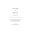
Figure 2.1 AlGaAs-type diode laser chip structure (Sharp Corp., Laser Diode
User's Manual, 1988)
6
schematic of the diode laser chip structure, showing details of the composite
materials and the radiation pattern. This cavity, by way of multiple reflections of
light from the end-faces (facets), and stimulated emission by electron-hole pairs,
produces the amplification necessary for lasing. The lasing radiation is emitted at
both facets of the cavity, which are cleaved plane surfaces of the semiconductor.
The rear facet of the optical cavity emits part of the total radiation, which
impinges on a built-in photodiode. This photodiode can be utilized as an indicator
of real-time lasing intensity.
The front facet of the cavity is the "working end" of the diode laser. The
radiation is emitted from this very small-dimension surface, causing this radiation
to diffract through a relatively large angle, necessitating the use of collimating
lenses.
For most of our work, we used Al GaAs-type diode lasers. An InGaAIP-type
visible diode laser was also used. Both types of lasers are a heterojunction
structure, and operate on the index-guided principle. These two types of lasers
have similar characteristics, therefore, only Al GaAs-type lasers are explicitly
mentioned in the following discussion.
For the Al GaAs-type diode lasers, some general numbers that are useful can
be realized: A typical diode laser cavity is about 0.3 mm long. The index of
refraction of the cavity is approximately 3.6. The reflectivity of the cavity endfaces may be around 30 percent, depending on whether anti-reflection coatings
are applied. The linewidths of free-running diode lasers are typically in the range
from 10 to 100 MHz.
7
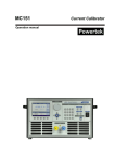
A very important characteristic of a diode laser is its threshold current value,
Ith.
Drive currents below 6 are not sufficient to maintain a minimum carrier
density required for lasing. These low currents will result in emitted light from the
cavity, but this light is merely a result of spontaneous emission, as for the case of
light-emitting diodes. The coherent, intense quality of laser emission is only
achieved when the current is above Ith. Beyond this threshold the light power
rapidly increases linearly with increasing drive current, as shown in Figure 2.2. A
common value for the slope of the stimulated emission part of the curve is 0.5
mW/mA.
a
I
stimulated
emission
spontaneous emission
Injection current I
Figure 2.2 Schematic view of the light output power versus current characteristics
of a diode laser (Petermann, 1988).
8
2.2 Wavelength Tuning
AIGaAs -type diode lasers are readily available in many wavelengths, over the
range of approximately 635 nm to 1000 nm. The diode laser bandgap is
engineered for a specific target wavelength by varying the type and amount of
material alloyed to the basic GaAs crystal. Typically, this target wavelength is
reached only within a few nanometers for each specific diode laser that is built.
Subsequently, each diode laser can be fine-tuned to a more precise wavelength
by adjusting the diode laser current, temperature, or both. Conversely, a
stabilized wavelength is only achieved by careful control of the temperature and
current. Roughly speaking, the change in frequency per change on temperature
is -20 GHz/K. The change in frequency per change in drive current is -3 GHz/
mA.
The diode laser wavelength's dependence on temperature is due to the
temperature-dependence of the optical path length of the cavity. Also,
temperature affects the wavelength-dependence of the gain curve. These two
temperature dependencies are very different from each other. For AI GaAs-type
lasers, the optical path length changes about 0.06 nm/K, while the gain curve
changes about 0.25 nm/K [Wieman, et al. 1991]. This temperature-dependence
mismatch results in, unfortunately, discontinuous wavelength tuning with
temperature. The spectrally-shifting gain curve creates these discontinuities
when the laser jumps from one longitudinal mode to the next. These jumps are
called mode-hops, and they are discussed in the next section.
9
Diode laser wavelength is tunable by current because the current affects the
diode laser temperature. Also, the current directly affects the diode laser's carrier
density, which affects the cavity's index of refraction, resulting in changes to the
cavity's optical path length.
2.3 Diode Laser Modes
Several laser modes exist within the gain curve of a diode laser. The
distribution of the intensity of the lasing modes depends on the spectral location
of the modes relative to the gain curve. A single-mode diode laser has a narrow
gain curve that ideally supports only one mode. In reality, more than one mode
will be present in the emission of any real laser.
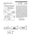
Figure 2.3 is an example of an emission spectrum of a 760 nm, index-guided
diode laser, sold as a single-mode device. For this spectrum, the operating
conditions of the laser were less than ideal resulting in secondary modes that are
clearly observable. The frequency separation of these modes is the free spectral
range (FSR) of the diode laser. The FSR is given by Ay = c/2nL, where c is the
speed of light, n is the index of refraction of the cavity, and L is the length of the
cavity. The FSR of diode lasers usually lies in the range of 50 - 150 GHz.
The ratio of the magnitude of the intensity of the primary mode to the intensity
of the second-most intense mode, is called the side-mode-suppression ratio
(SMSR). The value of this ratio indicates whether the laser is a "good" single-
10
REL. FREQUENCY (approx. 30 GHz per tick mark)
Figure 2.3 760 nm diode laser emission spectrum showing primary and
secondary modes. The free spectral range is 150 GHz.
mode laser. Good single-mode diode lasers may have a SMSR as high as 100.
For our experiments, as will be seen in Chapters 4 and 5, we operate the 760 nm
diode laser, of Figure 2.3, in a single mode, with an SMSR of approximately 60.
After consideration of the single mode lasing characteristics, one must be
aware that this single mode operation is highly dependent on a current and
temperature combination, for reasons explained in the previous section. Indeed,
a single mode oscillation will quickly digress to a multimode condition with
perhaps only a slight change in the diode laser's drive current, temperature, or
11
both. Then after a bit more change in this current and/or temperature, the laser
may once again operate in a (quasi) single-mode. This latter mode may be at a
different wavelength than the first. If so, then what has been described is a
mode-hop. Mode-hops may be jumps of one or more than one FSR of the laser.
These jumps greatly inhibit the usefulness of diode laser's wavelength tuning
utility, since the wavelength ranges within these jumps may not be accessible.
These wavelength-tuning gaps are unique for each specific laser. Thus shear
luck plays a large part in the procurement of these lasers for many wavelengthspecific experiments.
In addition to mode-hops, the diode laser may lase with comparable intensity
in two modes simultaneously. This condition is normally unstable, and is usually
the transient condition of a mode-hop, but with careful control of laser current and
temperature, two-mode operation can persist indefinitely.
2.4 Optical Feedback
Optical feedback of the laser field into the laser cavity has significant
consequences for the operation of the diode laser. These consequences may be
beneficial or detrimental. Quite often, carefully controlled feedback is used to
drastically narrow the linewidth of the laser, operate on a specific laser mode, or
tune to a specific frequency [Wieman, et al. 1991, Kitching, et al., 1994].
12
Unintentional feedback can dramatically degrade the spectral characteristics of
the laser.
The literature [Tkach, et al., 1986, Petermann, 1988] classifies the relative
magnitude of diode laser feedback into a four-regime hierarchy. Regime I is weak
feedback that may broaden or narrow the spectral width, depending on the
parameters of the feedback. Regime II may also result in line narrowing, but in
general, mode hopping and multiple cavity modes will exist. Regime Ill is similar
to regime II, but there is more feedback, and greater line narrowing. Finally,
diode laser operation in
regime IV guarantees highly degraded optical
performance, with spectral linewidths the order of 10 GHz with very large
amounts of intensity noise.
2.5 Diode Laser Noise
The spectral emission of diode lasers has neither constant frequency nor
constant intensity. The coherence length may be as short as a meter, depending
on many factors, including current and temperature stability of the diode laser,
mode stability, and the factors mentioned earlier in this chapter. Even under ideal
operating conditions, the diode laser emission contains noise. For this ideal case,
the primary source of noise originates from spontaneous emission, producing
both intensity and frequency fluctuations.
13
2.5.1 Diode Laser Noise Models
This section gives a brief review of the various statistical models of diode
laser noise found in the literature [See, for example, Raymer, et al., 1979, Elliott,
et al., 1988, Georges, 1980, Dixit, et al., 1980, and Ritsch, et al., 1990]. The work
of this thesis is only concerned with the phase-diffusion field model (PDM),
described below. For completeness, other models are briefly described, namely,
the thermal/chaotic field model, and the real Gaussian field model.
For a diode laser exhibiting only phase noise (no amplitude noise) the laser
E-field may be represented by the equation
E(t) = (1/2)Ei(t) exp[ -icoot ],
2.1
where coo is a well-defined center frequency, Ei(t) = E0 exp[- i4(t)], E0 is a constant,
and 0) is a fluctuating phase. For the PDM, 4(t) is a Gaussian random variable,
with zero mean, giving a field correlation function,
(E(ti)E(t2))= E02 exp[-F(t1 -t2)],
2.2
where F is the laser linewidth. The thermal/chaotic field model [Mollow, 1968]
takes the amplitude to be a complex random variable, with the phase being
constant. This model is closely approached by the radiation from a thermal
source of independent oscillators, or the radiation generated by a laer operating
on several independent modes. The real Gaussian field model [Elliott, et al.,
1988] is similar to the thermal/chaotic model, but the amplitude is considered a
real Gaussian variable.
14
2.5.2 Types of Diode Laser Noise
As mentioned above, diode lasers often emit light in more than a single mode.
Even so-called single mode lasers under optimum conditions will have a finite
amount of power distributed into secondary modes. Each of these lasing modes
has its own intensity noise characteristics, and so it is important to know whether
the full laser spectrum is detected or just a single mode. Ironically, the intensity
noise of the superposition of all the modes is usually a great deal smaller than
the noise for only a single mode. This situation is referred to as mode partition
noise [Petermann, 1988].
In order to explain the significance of mode partition noise, a quantity is
defined that relates intensity noise power to the mean power of the laser. This
quantity is called the relative intensity noise, or RIN. An example of mode
partition noise, in terms of the RIN, for a quasi single-mode laser, is shown in
Figure 2.4 [Petermann, 1988]. For this diode laser, with a SMSR of more than 20,
driven 20% above threshold, the RIN of the dominant mode alone is very high at
the lower frequency-end of the spectrum. The RIN decreases more than three
decades towards the higher frequency end of the spectrum. The RIN of the total
(all modes) laser emission trends the other way, starting with a rather small RIN
at the lower end of the spectrum. Thus the laser would have to be considered to
have a much higher RIN for applications that only utilized the dominant mode.
For instance, in spectroscopy, the dominant mode may be tuned within the
15
10-9
RIN of the
dominant mode alone
10-1°
10-11_
dominant
mode
10-12
838
836
10-13
X [nm)
RIN of the total laser emission
10-14
10-19
0.01
0.1
1
3
frequency IGHz1
Figure 2.4 RIN spectra for a GaAIAs diode laser, driven at 20% above threshold.
The side-mode intensity is less than about 5% of the dominant mode
(Petermann, 1988).
16
absorption envelope of an atomic transition but the secondary modes would be
completely detuned from the line by perhaps 150 GHz.
If the SMSR is relatively high, then the lower curve in Figure 2.4, describing
the total laser emission, can be used to describe the diode laser emission, even if
only the dominant mode is considered.
The total (integrated across the frequency spectrum) RIN varies greatly with
the drive current of the diode laser. A maximum RIN is reached at a drive current
slightly greater than the threshold current. Then as the current is increased, the
RIN decreases several orders of magnitude as soon as the drive current
increases to one and a half times threshold, shown in Figure 2.5.
Frequency noise is more prevalent than intensity noise under steady-state
operating conditions for the 760 nm diode laser used in the experiments. The
frequency noise almost entirely determines the spectral linewidth [Yabuzaki, et
al., 1991], for noise spectra far from the relaxation oscillation frequency, first
described in the following section. The frequency noise spectrum for a typical
diode laser is shown in Figure 2.6 [Yamamoto, 1991]. The local maxima are
relaxation oscillations.
Both frequency and intensity noise are essentially introduced by the same
spontaneous emission noise events, thus it follows that they are highly correlated
[Petermann, 1988]. However, this is not the case for diode lasers experiencing
an increased level of noise due to feedback. In this case the resulting "noise"
from the feedback is actually a manifestation of rapid fluctuations of the power
spectrum of the laser. This does not give rise to a high level of correlation
17
between
frequency
and
intensity
modulation,
though
the
feedback
simultaneously increases both.
10-12
1
10-13
10-14
0,8
1,2
1.0
I/Ith
1.4
1,6
-0.
Figure 2.5 Measured RIN of a GaAIAs diode laser versus drive current
(Petermann, 1988).
18
-2
10
1
108
r
i
I
1
1
10
2
Frequency
Figure 2.6 Frequency noise spectra for a typical GaAlAs diode laser. The solid
curves show different cases of drive current, and the dashed curve is similar to
the behavior of a diode laser obeying the phase diffusing model (Yamamoto, et
al., 1991)
19
2.5.3 Relaxation Oscillations and the Diode Laser Power Spectrum
For the diode laser, the two quantities of interest are the number of photons in
the cavity, S, and the number density of carriers, n. Two rate equations for these
quantities are [Petermann, 1988],
dS
dt
2.3
`J"'st
TI-Dii )-1- Rsp
and,
dn
dt
2.4
1
eV
R(n)
---L- S
V
where Rsp is the number of spontaneously generated photons per unit time of a
given laser mode, Tph is the photon lifetime,
Rst
is a stimulated emission
coefficient, R(n) is the recombination rate, I is the injection current, and V is the
volume of the active region.
Since the spontaneous emission noise exists across a large frequency range,
it can be considered to be a white noise source. A Gaussian distribution may be
used to describe its spectral probability density. Equation (2.3) is modified to
account for this noise source by adding a term, F(t), that represents a Langevin
noise source with zero mean value;
20
dS
= S(Rst
tr;t, )+ Rsp + F(t)
2.5
Laser linewidth varies inversely with output power as predicted by the
modified Schawlow-Townes formula [Schawlow, et al., 1958]. However, this
power dependence for diode lasers must be modified further by the simple
multiplicative factor (1 +a2), where a is called the linewidth enhancement factor
[Henry, 1982]. a is defined as the ratio of real refractive index fluctuations to
imaginary refractive index fluctuations in the active region. Henry showed that the
increased linewidth is due to the strong coupling between phase and intensity
noise.
The diode laser linewidth is given by
8v =
ithvnsp
2.6
(1 + a) 2
Ptot (27tTp )
where v is the lasing frequency, Tp is the photon lifetime in the cavity, Ptot is the
total emission power, and nsp is the spontaneous emission factor given by
nsp = {1
expRhv +Ev -E,)/kTr
2.7
21
where E, and Ec are the valence and conduction band quasi-Fermi levels, k is
the Boltzmann constant, and T is the temperature [Cartaleva, 1994, and Fleming,
et al., 1981].
The spectral lineshape of diode lasers includes sidebands first recognized as
relaxation oscillations by Vahala, et al. [1983], and expressed as part of the
spectral profile by van Exter, et al. [1992]. Relaxation oscillations (RO's) occur
due to an initial perturbation in the number of carriers and/or photons in the laser
cavity. Although RO's are a transient effect in gas lasers, they are a steady-state
condition for diode lasers. If the carrier density momentarily exceeds a threshold
value this will cause an excess of photons also exceeding a threshold. These
extra photons consume enough carriers to reduce the carrier population to below
the threshold level. This depleted condition of carriers results in a decreased
number of photons to below the threshold value. Due to this lowered photon
population the carrier density recovers enough to once again surpass the
threshold value. This cycle repeats, resulting in a ringing at the relaxation
oscillation frequency. RO frequencies are typically between 1.5 and 5 GHz.
The RO frequency increases with increasing drive current of the diode laser.
Temperature decreases will also increase the RO frequency. The square of the
RO frequency varies linearly with laser power, with a slope of approximately 2
GHz2/mW [van Exter, et al., 1992, Figure 6]. Also, higher-order RO's exist, but
their intensity drops considerably from one order to the next. Agrawal, et al.
[1993, Figure 6.14] determines the spectral lineshape of a diode laser using
rather detailed expressions for the laser field. Figure 2.7 shows this result. Notice
22
the key feature is that the relaxation oscillation peaks move away from the
central frequency as the laser power increases.
The fraction of power that is contained in the RO's varies greatly with the
specific laser, feedback and other operating conditions. For example, VVieman, et
al. [1991] has found this power fraction to be of the order of 1/1000 for nearinfrared (NIR) diode lasers and as much as 1/10 for the relatively new visible
diode lasers.
The RO peaks display an asymmetry in height; the low frequency RO peak is
larger than the upper frequency peak. Vahala, et al. [1982] believed this
asymmetry to be the result of the coherence between amplitude and phase
fluctuations. The intensity of the RO peaks' asymmetry has been correlated with
the linewidth enhancement factor a [van Exter, et al., 1992].
0
1
2
FREQUENCY, v
3
4
vo (GHz)
Figure 2.7 Spectral lineshape calculated for a single-mode diode laser operating
at 0.5 mW and 1 mW (Agrawal, et al., 1993)
23
CHAPTER 3: THEORY OF DIODE LASER PHASE NOISE AND
ITS CONVERSION TO AMPLITUDE NOISE
3.1 Introduction
In this chapter, we investigate the behavior of a diode laser field with phase
noise as it propagates through an interferometer, or an atomic medium, during
which the frequency of the laser
is
spectrally scanned across either a
transmission resonance of the interferometer, or an absorption line of the
medium. Specifically, we are interested in the spectral behavior of the intensity of
the transmitted field, which is measured by a square-law photodetector.
In general, we may write our laser electric field as
E(t) = Eo (t) cos[coLt + OA
3.1
where col_ is the laser center frequency, (I)(t) is a time-dependent phase noise, and
E0 (t) is assumed to vary little in an optical period 27t /coy. The photodetector will, in
general, measure an intensity which we separate into its time-independent and
time-dependent parts. As explained in Chapter 4, we use a radio frequency
spectrum analyzer (RFSA) to measure the time-dependent part of the intensity.
Because optical frequencies are too high (1014 Hz) for any detector to follow,
any contributions to a time-dependent intensity must come from Eo (t),
0), or
both. In our work, E0 (t), and 0) are the amplitude noise, and phase noise,
respectively, of our diode laser. In Chapter 5, Eo (t), and 4(t) are analyzed in the
24
frequency domain, which gives their spectra, primarily in the radio-frequency
range (106-109 Hz).
As above, consider Eo(t) and OM to have frequencies in the radio frequency
regime. By squaring equation 3.1, and taking the time-average over an optical
period, as a square-law photodetector does when measuring intensity, we obtain
1(t)
(Eo(t))2. As long as 4(t) varies slowly during the optical period the factor OM
is not in this final result. This indicates that one can directly measure the timedependence of Eo(t), the amplitude noise, but not that of OM, the phase noise.
The 760 nm diode laser used for the primary experimental work described
here should exhibit phase noise only [Yabuzaki, et al., 1991], and so we now set
E0 = constant. Since this phase noise cannot be measured directly, we must
convert it into amplitude noise in order to detect it. There are several ways of
performing this conversion, and the simplest way is using a two-beam
interferometer, explained as follows.
The laser field, after passing through a two-beam interferometer, can be
written
E(t,T) = E0 {cos[coLt + OA + coskoL(t-T) + (1)(t-t)ll
3.2
where t is the time delay of one beam relative to the other introduced by the
interferometer, i.e., t = AUc, where AL is the optical pathlength difference
between the two branches of the interferometer, and c is the speed of light.
25
Squaring and time-averaging equation
3.2
results in a time-dependent
intensity due to the phase noise;
Idet(t,t) = 10/2 {1 + cos[-cocr + 6,(1)(t,c)l}
where All)(t,t) = 4(t)
(1)(t
3.3
t), and lo is E02. This process of mixing two fields with
different phases, and thus converting phase noise to amplitude noise, is a type of
heterodyne detection. In this thesis, this process will be called simply
"heterodyning".
We now determine the heterodyne intensity, Idet(t,t), as a function of the
relative phase delay, (ALT, introduced by the interferometer. Using an angle-sum
trigonometric identity, equation 3.3 becomes,
Idet(t,t) =
10/2{1 +
[cos(A(p)cos(om)
sin(i 0)sin(a)Lt)]}
3.4
Next, we expand cos(A(p) and sin(AT),
Idet(t,t) =
10/2{1 + [(1
(AT
AT2/2! +
AT3/3! +
44/4! ...)cos(an) +
AT5/5!
-...)sin(oyr)]}
3.5
Let us assume our laser is not very noisy so that 60 is small. We then ignore all
4-terms which are higher order than one;
Idet(t,T) =
10/2{1 + [COS(COLT)
.6p(t,t)sin(cocr)] }.
3.6
As COL is scanned, as described in the first paragraph of this section, the first
two terms of equation 3.6 yield the characteristic two-beam interference pattern
for a perfectly monochromatic light source, i.e., AT = 0. When COLT = 2m7c, where
m is an integer, an interferometer transmission maximum is obtained. At these
values of col_ the third term in equation 3.6 goes through zero, changing sign.
However, a RFSA measures magnitudes of the Fourier components of AT;
26
therefore, the signal measured by a RFSA is always positive definite, and simply
vanishes when cocc = 2m7c. Thus, as the laser is tuned through an interferometer
resonance, the RFSA signal yields a spectrum termed an "m-shape".
We now treat the more general case of a multiple beam interferometer, or an
atomic/molecular vapor or gas. To do so, we introduce the Fourier spectrum of
the phase noise, A4)(t,t). We first use a graphical representation to illustrate the
character of the phase noise spectrum of the laser field, and in the following
section we rigorously develop more general expressions of the noise spectra,
modeling the noise as a modulation.
To obtain a graphical representation of phase modulation, we first examine
the graphical representation of amplitude modulation. A single-frequency
amplitude modulated laser electric field can be written
EAM(t) = (1 + 2McosQt)cosokt
3.7
where M is a modulation index (the factor 2 is for notational convenience), Q is
the modulation frequency and OIL is the laser field central, or carrier, frequency.
Rearranging equation 3.7,
EAM(t) = cosekt + M cos[((.k + S2)t] + M cos[(coL S))t]
3.8
We can represent equation 3.8 graphically by using rotating vectors, or
phasors, as in Figure 3.1a. The resultant phasor rotates with a constant angular
velocity, coo, but its magnitude varies cyclically.
27
A single-frequency phase modulated field can be written
3.9
EpM(t) = cos(coLt + Moos Qt)
where M is a modulation index, and Q is the modulation frequency. Equation 3.9
is much more complicated than equation 3.7, so we will start with the phasor
representation in order to find a simplified expression for equation 3.9. At this
point, we note that in order to implement the phasor representation for phase
modulation, we have 0«ok, and M <<1, as in our work. With these conditions on
Q and coL, the phasor representation is shown in Figure 3.1b. By inspection, it
can be seen that this phasor picture is the same as the one in Figure 3.1a, for
amplitude modulation, with the only difference being that one of the smaller
phasors is flipped it radians. The resultant phasor of the two small phasors is
coo + C2
a)
oo Q
b)
wo + Q
> 0) 0
Figure 3.1 Phasor representation of a) amplitude modulation, and b) frequency
modulation. These phasors are rotating vectors that rotate with the angular
frequency noted on each vector.
28
orthogonal to the large phasor at all times. This orthogonality contributes to a
cyclically varying angular frequency of the final resultant phasor. This is only an
approximation based on the fact that Q is much smaller than coo, otherwise this
phasor picture gives us simultaneous phase and amplitude modulation. However,
with this approximation, the phasor representation of Figure 3.1b tells us that we
can write equation 3.9 as
EPM(t) = cosc.ikt + M+ cos[(oh. + qt]
M_ cosRok QM
3.10
where the coefficients of the second and third term are labeled differently for
generality (This is justified since equation 3.10 is based on the approximate
phasor model in Figure 3.1b, whereas equation 3.8 is exact, so we have no
leeway in assigning our choice of coefficients.). Here, M+ and M_ are positive,
constant amplitudes.
Equations 3.8 and 3.10 are represented in the frequency domain by the
schematic model shown in Figure 3.2. The vertical lines represent the
frequencies and magnitudes, including some phase information, of the Fourier
components of the field. For instance, in Figure 3.2b, the central frequency
component at coo has the largest magnitude of the three terms shown, and is
called the carrier frequency. The other two frequency components, at coo + S2 and
wo
0, are called the upper and lower sidebands, respectively. The lower
sideband is shown to be equal in magnitude with the upper sideband, but these
two fields differ in phase by Tr radians. The case in Figure 3.2a is similar, but both
sidebands are in phase with each other. We relate this schematic model with
equation 3.8 and 3.10 as follows. The carrier frequency is the first term of
29
coo -c
>0)
(00 -S2
coo
coo +
(a)
>0)
coo
(b)
Figure 3.2 Frequency-domain representation of the rotating vectors in Figure 3.1,
for a)amplitude modulation, and b) frequency modulation.
equations 3.8 and 3.10, with unity magnitude, and the upper and lower
sidebands are the second and third term, respectively. The coefficients of the
second and third terms, M+ and M_ are equal. Equations 3.8 and 3.10 represent
figures 3.2a and 3.2b, respectively.
The field of equation 3.8 is squared, and time-averaged by a detector,
resulting in a heterodyne signal. However, squaring, and time-averaging the field
of equation 3.10 gives a heterodyne signal of zero, as expected, since M << 1,
30
and we ignore terms involving M+M_, M+2, and M2. However, if the coefficients,
M+ and M_ are no longer equal, then we will get a heterodyne signal. For
instance,
if the
upper sideband
is
selectively
transmitted through
an
interferometer, more than the lower sideband, then M., > M_. This is the crucial
principle underlying heterodyning detection.
In the remainder of this section, we show how a heterodyne m-shape is
produced as the laser field frequency, represented by the carrier/sideband
picture, is scanned across a resonance feature. We use the term "beating",
referring to the resultant difference frequency one gets when mixing two
frequency fields.
The discrete, single-sideband model introduced above is useful because of
how we measure the heterodyne signal; we use a RFSA that is set at a specific,
tuned frequency, f2. As above, to a first approximation (the character of this
approximation is explained at the end of this section), we consider the laser field
to consist of a principle, or carrier, frequency, and an upper and lower sideband.
Each sideband is separated from the carrier by the frequency of the tuned
spectrum analyzer, SI. These three frequency bands will beat with each other as
they are mixed on a photodetector. The possible beat combinations are the
beating of the carrier with either of the two sidebands. It is important to note that
the carrier will beat with both the upper and the lower sideband, and the beat
frequency will be the same for both cases. However, there is an opposite phase
between these two beats, since the upper and lower sidebands are out of phase
by n radians. Opposite phase causes these sideband beats to cancel.
31
The upper part of Figure 3.3 depicts the carrier and a pair of sidebands as
they are scanned across an atomic/molecular absorption line. The lower part of
the Figure shows the resulting heterodyne lineshape at every point during the
scan. We now explain how we arrive at this result.
As the laser field's frequency is adjusted so the three frequency bands begin
to move into the absorbing feature, in Figure 3.3, the upper sideband will be
TUNING -
Figure 3.3 Carrier and sidebands tuned across an absorption line (top) give the
heterodyne m-shape (bottom).
32
attenuated more than the lower sideband, and the sideband beats can no longer
cancel. A resulting net beat signal becomes a heterodyne signal when the two
beating frequency bands mix on the surface of a square-law photodetector. The
photodetector converts the light intensity into a photocurrent. An oscilloscope or
spectrum analyzer can measure this photocurrent which includes the beat
frequency. As the laser continues its scan into the absorbing feature, the
heterodyne signal continues to grow as the imbalance of the sideband
magnitudes increases. As the scan takes the laser frequency near the center of
the absorption, the two sidebands begin to experience similar attenuation, and
the heterodyne signal falls to zero at line center. The scan continues into the far
side of the absorption feature, and the sideband imbalance resumes, again
giving a heterodyne signal until the laser is scanned past the absorption region.
The heterodyne lineshape from the above sequence is clearly an m-shape. A
similar situation occurs if the carrier and sidebands are tuned across an
interferometer transmission resonance instead of an absorption resonance.
In the example above, only the first-order pair of sidebands, at col_ ± f2 is
considered. However, as we will see in the following section, a Fourier analysis
of equation 3.9 yields sidebands at 0L ± 252, oh. ± 352,
± 4S2, and so on, The
RFSA, operating as a tuned receiver, will respond to the modulation frequency,
and all harmonics that are multiplicative factors of this frequency. As an example,
if the spectrum analyzer is tuned to receive a modulation frequency of 10 MHz
then it will measure all components of 10 MHz, including the second harmonic of
the 5 MHz Fourier component, the third harmonic of the 3.33 MHz component,
33
and so on. However, the even-numbered harmonics do not contribute to the
overall heterodyne signal of interest, due to a detail of the nature of frequency
modulation; every even-numbered sideband pair is comprised of sidebands that
are in phase with each other. Thus these pairs contribute to the heterodyne
signal without the need for a spectrally absorbing feature. Being independent of
the spectral feature of interest, these sideband pairs produce a background
signal. Typically, the magnitudes of the sideband harmonics quickly diminish as
their frequency moves away from the carrier frequency, so their contribution to
the heterodyne signal is negligible.
3.2 Mathematical Description of Phase Modulation
If the amplitude or frequency of a sinusoidal function has time dependence,
the resulting signal is best described in terms of a Fourier series of frequency
components [Cuccia, 1952, Rowe, 1965, and Black, 1953]. Repeating equation
3.1, for a laser field,
E(t) = Eo(t) exp[ i(oLt
(1)(0)]
3.11
Here, we set Eo(t) = E0 = constant . For notational clarity, let ooy in equation 3.1 be
written coo.
In order to develop a mathematical description of phase modulation, we begin
with the case of no amplitude modulation and a sinusoidally modulated phase:
0(t) = 13sin comt
3.12
34
where 3 is the modulation index and com is the modulation frequency. (In section
3.1, corn was called 0). For the present case, equation 3.11 is written
E(t) = E0 exp[i(coot + psin comt)]
3.13
E(t) = E0 exp[ipsin (DA exp icoot
3.14
or,
keeping in mind that E0 is a constant. The first exponential factor can be written
as a complex Fourier series,
exp[i[3sin court] =
C. exp[incomt]
3.15
n=co
where the Fourier coefficients are,
It
C
n
= ---r"c° .F. exp[ipsincomt]exp[incomt]dt
2 7c -I.,
3.16
The solution of the integral in equation 3.16 yields Bessel functions for the
Fourier coefficients;
Cn = Jii GI)
3.17
E(t) = Eo EJ,, (P)exP[1(0)0 + ncom)t]
3.18
So finally we have
Equation 3.18 is the general expression for single-tone frequency modulation. By
inspection, it can be observed that equation 3.18 is composed of a carrier and an
infinite number of sideband pairs, as shown in Figure 3.4. All neighboring
sidebands are separated by corn. Notice the odd-numbered lower side bands are
phase inverted. This results from the equation [Cuccia, 1952, appendix has a
nice treatment of Bessel functions in the context of modulation theory]
35
J_n
(3) = (-1)n Jn (3)
3.19
Also, the magnitude of the sidebands decrease as they move farther away from
the carrier. The character of this sideband spectrum depends on the modulation
frequency and index. Supplee, et al. [1994] review the effects of these
parameters on frequency modulation spectroscopy.
Although frequency noise dominates amplitude noise in diode lasers, the
noise modulation effects due to their coexistence can be realized by investigating
the results of replacing E0 in equation 3.13 with
E0(t) = (1 + Mcoscot)Eo
3.20
In order to simplify the analysis, the cosine term adds an amplitude modulation of
the same frequency as the frequency modulation.
Wm
coo
Figure 3.4 Carrier and sidebands for single-tone frequency modulation
36
Realizing that
co
exp[ipsin omt] = E,In (p) exp[incomt]
3.21
Equation 3.18 can be written in a final form;
E(t) = Eo{ i Jn(P)eXPi(00 ± mom )t +
I-; °±Jr,(8)expi(wo +(n +1)com )t +
M
2,i -In (R)expi(coo + (n 1)com )t]}
3.22
This spectrum is shown in Figure 3.5. There is now a lack of symmetry between
the upper and lower sidebands. The upper sidebands will always be greater on
average than the lower sidebands. Some of the spectra of optical heterodyning
display this asymmetry, as will be seen in Chapter 5 of this thesis.
com
(0o
> 0)
Figure 3.5 Carrier and sidebands for simultaneous frequency and amplitude
modulation.
37
3.3 Using a Lummer-Gehrcke Interferometer to Measure Laser Phase Noise
3.3.1 Motivation
For a laser emission obeying the phase-diffusing field model presented in
section 2.5.1, theory predicts a heterodyne lineshape to be the double-peaked m-
shape, presented in section 3.1. Also, the peaks of the m-shape are predicted to
be of equal height, a condition for which we will use the term "symmetric". Earlier
heterodyne work with rubidium [McIntyre, et al., 1993, and McIntyre, private
communication] resulted in asymmetric m-shapes. It was noted [McIntyre, et al.,
1993] that this asymmetry was largely attributed to the multilevel nature of the
transitions they were working with, though another cause for asymmetry is the
presence of amplitude noise in the laser emission. This rubidium example begins
to illustrate the difficulties that arise when heterodyning with an atomic or
molecular medium. Complications include optical pumping of ground-state
hyperfine levels, homogeneous and inhomogeneous broadening mechanisms of
the atomic/molecular gas or vapor, and selective reflection. Therefore, our work
begins with the simplest case of heterodyning, using an interferometer.
We have seen (section 3.1) that a heterodyne lineshape of an interferometer
is a symmetric m-shape, if the laser noise is described by the phase-diffusing
model (PDM), i.e. amplitude noise is not present. In anticipation of the more
complicated heterodyne work with molecular oxygen, we investigate the
character of our diode laser emission, which we will later use for the oxygen
38
work, by using this laser for interferometer heterodyning. To see if this diode
laser's emission obeys the PDM, we look for symmetric m-shapes.
A final concern with the character of the diode laser emission is that we want
to ensure that this emission is not affected by any parts of the experiment
external to the diode laser, such as optical feedback. For this reason we avoid
using a Fabry-Perot interferometer, which has been known to result
in
asymmetric m-shapes [McIntyre, personal communication], perhaps because a
properly aligned Fabry-Perot interferometer will reflect light back into the laser
cavity. Below, we describe the interferometer that we use.
3.3.2 Lummer-Gehrcke Interferometer
A Lummer-Gehrcke interferometer (LGI) is a multiple-beam interferometer. It
is a rectangular slab of quartz with a prism optically fused to one of the larger
surfaces of the plate, as illustrated in Figure 3.6. A beam of light enters the
Figure 3.6 Lummer-Gehrcke interferometer
39
vertical face of the prism, at an angle far from orthogonal to this surface, thus
avoiding any possibility of optical feedback into the diode laser. The beam is then
internally reflected from the diagonal face of the prism. Subsequently, the beam
enters the slab and repeatedly internally reflects from the top and bottom
surfaces, as a result of (almost) total internal reflection. The function of the prism
is to allow the beam to enter the slab at less than the critical angle so that total
internal reflection can occur.
For proper interferometric operation to occur, the beam in the slab must be
internally reflected at slightly less than the critical angle, resulting in a small
fraction of the beam exiting the slab (transmission at the interface) at every
reflection. Concomitant with the multitude of internal reflections is a number of
exiting beams, each one phase-delayed consecutively from the next. The phase
delay is a result of the additional distance the internal beam travels during the
next two internal reflections.
The exiting beams emerge from both the top and bottom surface of the LGI at
a near-grazing angle, though only one surface is utilized. Exiting the surface of
the plate, all the beams are parallel to one another, requiring a converging lens,
or beam divergence, so the exiting beams overlap and interfere with each other
on a screen or detector.
40
The intensity distribution of the interference pattern of the LGI, at the detector,
is given by [Born and Wolf, 1965]
1+ GP sine
P5
2
9ip)21
3.23
1+ Fsin2 5
2
where
F
491
(1-91)2
3.24
and
GP =
49p
(1 -91P)2
3.25
5 is the phase difference between successive beams, 91 is the reflectivity inside
the plate interface, p is the number of exiting beams, and I is the intensity at the
detector with the LGI removed. The finesse,
f,
is defined as the ratio of the
separation of adjacent fringes to their FWHM, and f = (7c/2)Fl1 2. Figure 3.7 shows
the plotted spectrum of equation 3.23 for several different values of p. It is similar
to an Airy function modified by the sinusoid in the numerator. The result is the
occurrence of subsidiary maxima between the usual Airy maxima. These
subsidiary peaks diminish as the number of exiting beam contributions increases.
As p approaches infinity, equation 3.23 approaches the usual Airy transmission
function associated with the common Fabry-Perot Etalon.
In Appendix A, some useful relations are derived for the LGI.
41
p = 25
0.8
p = 15
0.6
0.4
0.2
1111141411411
1414
-6
-4
-2
4141
0
I
2
i
4
6
d
Figure 3.7 LGI output spectra for several values of exiting beam number,
calculated using equation 3.23.
42
3.4 Lummer-Gehrcke Heterodyning
A simplifying approach to analyzing the LGI heterodyne spectrum is the twobeam approximation. In this case, only two of the many exiting beams of the LGI
are considered, and we can use the results of section 3.1. Thus, a LGI
heterodyne spectrum
is
the
symmetric m-shape, centered
at the
LGI
transmission resonance. The center of this m-shape, the central minimum, goes
to zero in this approximation. In other words, at exact resonance the heterodyne
signal is zero.
We now treat the case of a general number of interfering beams of a LGI. In
principle, we can predict a heterodyne spectrum for the LGI using equation 3.23,
by replacing 8 with 8 + Ay, where Acp = Ay(t) carries a time dependence that can
be measured by a spectrum analyzer. However, this approach is mathematically
non-trivial, since Ay represents a Fourier series of very many terms. In Appendix
B a treatment of a general number of LGI beams is given. The resulting
heterodyne intensity equation is very similar to equation 3.6, indicating that the
many-beam case also gives the result of a double-peaked heterodyne m-shape
centered at resonance. Quantitative predictions of the relative magnitudes of the
peak heterodyne intensity and the central minimum intensity would require the
incorporation of a proper diode laser noise model, such as the PDM, along with
the transmission function of the LGI. This analysis is beyond the scope of this
thesis, but it is a topic for future research. For our work now, the usefulness of
the qualitative theoretical predictions of symmetric m-shapes is enough to allow
43
us to characterize the emission of our diode laser and to ensure that it obeys the
phase-diffusion model.
3.5 Heterodyning with an Atomic/Molecular Vapor or Gas
3.5.1 Introduction
By using a diode laser for heterodyne spectroscopy of an atomic or molecular
medium, one takes advantage of the frequency noise that is always present in
these lasers. External frequency modulation of the laser injection current is not
needed.
A heterodyne signal is produced as the diode laser field jumps in and out of
resonance with an atomic line. The condition for macroscopic dipole polarization
is much more favorable as the laser field's frequency approaches resonance.
When this incident field jumps into resonance, a polarization is set up in the
medium that oscillates at -medium = (AE/h), where AE is the energy of the atomic
line transition and h is Planck's constant. When the diode laser field jumps out of
resonance, the polarization that was set up in the medium originally, oscillating at
- medium, continues to "ring", albeit with an exponentially decaying amplitude due
to dephasing mechanisms such as collisions. The polarization field and the
present incident laser field beat with one another as they mix at the surface of a
photodetector.
44
As a manifestation of phase noise, the optical field of a diode laser jumps
around in frequency space. A typical diode laser linewidth of 100 MHz implies a
coherence length of several meters. This is long enough to enable a perfectly
coherent wave train to encompass the entire length of a gas cell filled with an
atomic or molecular medium. The medium will experience a new singlefrequency coherent field as the diode laser jumps to a new frequency. A
requirement for heterodyning of the atomic medium is that the lifetime of the
macroscopic polarization be at least as long as the coherence time of the laser,
so that the polarization field and incident laser field can coexist.
As discussed in the first part of this chapter, section 3.1, an atomic or
molecular absorption line will give us a heterodyne m-shape. The character of
this m-shape, such as the width, central minimum value, and peak value, is
predicted by the phase-diffusing model (PDM) theory of Cooper, et al. [1990].
With this theory, the profile as a function of laser detuning is dependent on the
spectrum analyzer frequency, the natural linewidth of the medium, and the laser
linewidth.
One may realize a familiarity in the description above of the process of
heterodyning with an atomic medium to that of coherent transient experiments,
such as optical nutation and free induction decay [Sargent, et al., 1974, Brewer,
et al., 1972, Yong-qing, et al., 1996, Dube, et al., 1996, and Brewer, et al., 1976].
The crucial comparison is the beating of the incident field with the field of the
induced polarization of the sample. A difference is that heterodyning with a diode
laser gives the needed frequency shifts into and out of resonance automatically.
45
There is no need to Stark shift the sample into or away from resonance, or to
modulate the laser frequency externally.
The molecular oxygen absorption lines we are working with are in the electric
dipole forbidden b1E+9(v'=0).X3E-9(v"=0) band known as the A-band of oxygen
[Babcock, et al., 1948, Kroll, et al., 1987, Ritter, et al., 1987]. This band is shown
in Figure 3.8. The transitions then are primarily magnetic dipole [Garstang, 1962],
yielding a very small linestrength of about 9x10-10. This is readily calculated from
the Ladenburg relation [Corney, 1977];
f
4E 0 meck20
87te2T
3.26
where me is the electron mass, e is the electron charge, c is the speed of light, X.0
is the resonance wavelength, co is the permittivity, and Tr) is the natural lifetime of
1.0r
"
11,
r,
r.y
-Kri
11,
0.9-
0.r0.6'
0.5.
0.41.
0.3'
0.2
Pbranch -
0.1768
766
764
.
762
- Rbranch
760
WAVELENGTH (nm)
Figure 3.8 Calculated transmission spectrum of oxygen (Kroll, et al., 1987).
46
the transition, (approximately 10 seconds). These A-band transitions are two
level transitions, which the PDM-based heterodyne theory assumes. This theory
also assumes that the only dephasing mechanism of the absorption medium is
the natural lifetime decay, neglecting consideration of interatomic collisions. In
the case of the forbidden oxygen A-band transitions, the natural lifetime is so
great that the dominant dephasing mechanism is interatomic collisions. In the
next section we discuss the PDM heterodyne theory, and show that sum of
collision broadening and natural broadening can replace just natural broadening,
in the theory.
3.5.2 Heterodyne Theory for a Diode Laser Emission Obeying the PhaseDiffusing Model
The PDM-based heterodyne theory is based on the development of a phase-
diffusing laser field as
it
propagates through a resonant two-level medium
[Cooper, et al., 1990]. The theory considers the inhomogeneous Doppler
broadening of the medium. As the modified laser field is incident on a square-law
photodetector, a heterodyne signal is predicted by the theory, and measured by a
tuned-frequency RFSA. This heterodyne signal is integrated over the Doppler
distribution of the medium. A final step in the development of the theory is a
Fourier transform from the time domain to the frequency domain.
In the theory, the parameters needed to predict the heterodyne spectra are
the spectrum analyzer frequency,
co,
the laser detuning from the atomic
resonance, A, the natural linewidth of the atomic medium, y, and the laser
47
linewidth, F. In our work with oxygen, with very long lifetime transitions, the
collision linewidth is dominant over the natural
linewidth, and
Doppler
broadening. Therefore we add the collision linewidth to the natural linewidth, as
Schuurmans shows when he introduces interatomic collisions to his calculation of
the polarization of a gas [Schuurmans, 1980], and use this resulting parameter in
the theory.
In this thesis we apply an incomplete PDM-based heterodyne theory to our
oxygen work; we ignore Doppler broadening. This is justified because, as
mentioned in the previous paragraph, we include collision broadening instead.
The following equation is the theoretical heterodyne intensity with no Doppler
broadening [J. Cooper, private communication]:
/(A) a
(y +F)
F
7[A2+(r+1)2]{{(0 +A)2 +(7 +r)21
FRy + F)2 (2F + y )
[A2
+F)2]2L.-
A2 (4F + 3y )]
2
f
+
[00
(y +I-)
}+
1+
AY +(7 +r)2]]
(y + F)
+
[(co +0)2 +(y +r)2]
a +(y ( + 2F)2]
+(7
AF[(y +F)(5F +3y)- A2]
{
r)2 ]2 [A2
[A2
+ 2F)2] [(w
+(7
(y + I")
A)2
±r)2]) ±
A)
(w + A)
0)2 +(y +F)2]
[(w + 0)2 +(y +F )2 i
(co
1
3.27
In Chapter 5 we set y equal to the collision linewidth, and compare our
experimental results with the theoretical results of this equation.
We now show that equation 3.27, which was derived without integrating over
a Doppler distribution, may only modify the theoretical results slightly, even for
48
the case of Doppler broadening dominant over collision broadening. For this case
we use a rubidium transition with a natural linewidth of 6 MHz. At room
temperature the Doppler width is 570 MHz, and collisional broadening can be
neglected because the vapor pressure is very low. Figure 3.9 compares several
characteristics of a single peak of the heterodyne m-shape, using parameters for
rubidium, predicted by the theory with and without the Doppler integration. In the
case without Doppler integration, the Doppler linewidth is used for y instead of
the natural linewidth. In doing this, Doppler broadening is considered by the
theory but the Doppler frequency distribution is ignored. Peak heights and central
minimum heights for the cases with Doppler and without Doppler considerations,
shown in Figure 3.9a, are normalized to unity at zero RFSA frequency. In Figure
3.9b, both cases of FWHM are set equal at zero RFSA frequency, as is also the
situation for both cases of center width.
Differences between considering Doppler integration or not, shown in Figure
3.9, are noticeable, but not drastic. There is much more work involved in
producing the plots from the theory that includes the Doppler distribution
compared to simply using equation 3.27. So one may seriously consider whether
the slightly-increased accuracy is worth the extra effort .
The usefulness of equation 3.27 for the case with rubidium, in the previous
paragraph, gives us confidence of the validity of using this equation for
theoretical comparisons with our oxygen data, since Doppler consideration are
less important for oxygen than rubidium.
49
Peak Heights
without Doppler
0.8
Co
co
a) 'E
u.6-
CD
0.4-
a
.
N
tt3
Ta
0.2
0
z
with Doppler
0
0.5
0
1
1.5
2
2.5
RFSA Freq. (In units of the Doppler width, D: D=570 MHz)
Central Minimum Height
0.8with Doppler
0.6a)
'cE
a)
cm
U
o :E
0.4
_NJ -5
E
z8
without Doppler
0.2
0
0
0.5
1
1.5
2
2.5
RFSA Freq. (In units of the Doppler width, D: D=570 MHz)
Figure 3.9a Calculated heterodyne peak height (top) and central minimum height
(bottom) of rubidium with and without Doppler integration, versus spectrum
analyzer frequency.
Lc)
C\I
c\I
\
L.c,
N
.--
z
LO
C)
(zHN) Aouenbeid
C:)
LC)
C\1
C\1
LC)
'
N--
C:)
50
Figure 3.9b Calculated heterodyne FWHM and center width of rubidium with and
without Doppler integration, versus spectrum analyzer frequency.
51
3.6 Selective Reflection as a Possible Source of Optical Feedback.
In our work with oxygen gas, we shine the diode laser beam into a gas cell
which has quartz end-windows, as fully explained in Chapter 4. This arrangement
can produce unwanted optical feedback into the diode laser from reflections from
the gas itself, by a phenomenon called selective reflection (SR) [Schuurmans,
1980]. When light is incident on the interface between a dielectric and an atomic
medium, the Fresnel reflectivity of the interface changes as the light frequency is
tuned across an atomic resonance. This resonance modification of the reflectivity
occurs mostly within a few GHz of line center, as shown in Figure 3.10.
The spectral dependence of SR is double-peaked at resonance, resembling a
heterodyne m-shape. Therefore, feedback into the diode laser, from SR, can
increase amplitude and phase noise, enhancing the heterodyne m-shape peaks
1
-4
4,--2
).
0
2
Detuning (GHz)
Figure 3.10 Schematic of selective reflection versus detuning.
4
52
beyond what they would be if the only phase noise in the laser emission were
from the unperturbed laser. Thus, SR, if present, will be a complication in
comparisons between our measurements and the PDM-based heterodyne
theory. However, as discussed in Chapter 4, null results of experimental tests for
the presence of selective reflection effects allow us to ignore SR in our present
work.
As described in Chapter 4, even though the end-windows of our oxygen cell
are tilted to prevent Fresnel reflection from traveling back in the direction of the
laser, SR creates a backward wave that travels back towards the incident beam,
regardless of the angle of incidence on the reflecting surface. This situation is
depicted in Figure 3.11.
SPEC ULAR
REFLECTION
GAS CELL
SELECTIVE
REFLECTION
INCIDENT
LASER BEAM
QUARTZ
WINDOW
Figure 3.11 Graphical depiction of directional differences between specular and
selective reflection.
53
In the work of this thesis, there is no way to ensure that selective reflection is
not fed back into the diode laser. An optical isolator could be placed between the
laser and the oxygen cell's front window, but reflections from the optical isolator
will occur without the use of anti-reflection coatings designed for the wavelength
for which the optical isolator is used. For the present work, an optical isolator
designed for the proper wavelengths was not available for our use.
For the interested reader, the following is a brief survey of recent work on SR.
The concept of SR has been known since the early part of the twentieth
century [Wood, 1909]. A significant milepost of SR was made much later by
Cojan [1954] when he observed sub-doppler features in the selective reflectance
and related these to interactions of the atomic medium with the window (wall
collisions). Arguably, the beginning of the modern age of SR studies began with
the work of Woerdman, et al. [1975], and Schuurmans [1980]. Schuurmans and
Woerdman carried out detailed studies of the sub-doppler characteristics of SR
and demonstrated that they originate in the interruption of the optical dipole
phase by atom-wall collisions, and to the subsequent transient response of
ground-state atoms departing from the surface. Current research in SR involves
its use as an investigative tool to study atom-surface interactions [Ducloy, et al.,
(1991)], the study of SR in the dense atomic vapor regime [Guo, et al., 1996], SR
as a powerful spectroscopy tool [Wang, et al., 1997], SR as a function of
incidence angles [Nienhuis, et al., 1988], SR as a function of incident intensity
[Friedberg, et al., 1990], and SR in a pump-probe scheme [Schuller, et al., 1991].
54
To this end, Wang, Gallagher, and Cooper profoundly state the following
[Wang, et al., 1997]: "Selective reflection was first observed at the beginning of
the century, but it remains a complicated phenomenon for atomic physics theory.
A seemingly simple SR experiment may involve many physical processes that
are interleaved in the observations, making it a challenge to obtain an accurate
theoretical model."
3.7 (Optional) Heterodyne Detection and the Correlation Function
In this section, heterodyne detection is explained in terms of the correlation
function, which may be more familiar to the reader than heterodyning. In the
present case, the correlation function is used to measure the degree of
coherence of a laser field.
Essentially, optical heterodyning is the process of mixing light at a detector.
The light being mixed may have originated from the same light source, perhaps
passing through an interferometer, or the light may originate from different
sources altogether, as in the case of the application of a local oscillator. The
process of detection squares and time-averages the sum of the fields of light that
are mixed. The
individual fields,
in
general,
have
different amplitudes,
frequencies, and phase.
An application of the utility of heterodyne detection is the measurement of the
degree of coherence of a light source, such as the laser [Pedrotti, et al., 1993]. A
simple way of illustrating this point is to analyze the situation of a partially
55
coherent laser beam travelling through an interferometer. For simplicity, this
interferometer's output consists of only two beams. These two output beams can
be described by the complex fields El, and E2, respectively, and let E2 be time-
delayed by the interferometer, with respect to El. These fields then mix at a
photodetector. The photodetector squares and time-averages the sum of the
fields, to give the intensity,
1= ((E1 -FE2) (E1*÷E2)),
3.28
assuming the fields have identical polarization. Expanding,
1= (1E112+1E212+ (EIE2* + E1 *E2)),
3.29
1=11 +12 + 2 Re (EiE2*),
3.30
Or,
where 11 and 12 are the intensities of the individual fields. The third term of
equation 3.30 represents the interference of the two fields. The interferometer
introduces a time delay, T, between the two fields. The interference term of
equation 3.30 forms the basis of what is called the correlation function, y,
7 ==-- (Ei
(t)E2*(t
r)).
3.31
If both fields, El and E2, are identical except for their phase at the detector, then y
is called the autocorrelation function.
56
It is easily demonstrated that heterodyne detection measures the correlation
function, if the fields are written (compare to equation 3.2),
3.32
E1 = Eoexp{ikot-cp(t)ll
E2 = Eoexp{i[co(t
3.33
t)-90 TM.
This implies that the interferometer delays one beam relative to the other, without
dissimilar attenuation. This loss of generality does not change the character of
the results below, but merely simplifies notation.
For optical frequencies, we use equations 3.32 and 3.33 in equation 3.30 to
get
1(t) = 11 + 12 + 2E02 Re {exp{ipcot + (p(t)
(p(t
T)] }}
3.34
or,
1(t) = IDC + 10 cos pot + Acp(t,T)1
3.35
where the change in phase in time T is (gt,T) -=- cp(t) - cp(t - T), 'DC is the constant,
time-independent part of the intensity, and 10 is the amplitude of the varying part
of the intensity due to the interference. AT is a function of both t and T, since the
change in phase is clearly dependent on the path difference delay, and the
phase of the source is a function of time. Note that equation 3.35 is the same as
equation 3.6.
57
CHAPTER 4: EXPERIMENTAL TECHNIQUES
The work of this thesis involves several experimental configurations, depending
on the type of measurements performed. The experimental technique for
heterodyne spectroscopy with a LGI, and the similar technique used for work with
oxygen, will be discussed in this chapter. Direct AM noise measurements use a
technique that is different from FM noise detection, and this is also discussed in
the present chapter. Major parts of the experimental apparatus include a diode
laser, diode laser drive current control system, diode laser temperature control
system, the photodiode detection system, the oxygen cell, the LGI, data
acquisition and control of the experiment by a computer, the radio frequency
spectrum analyzer, and various beam-steering optics and focusing lenses. The
present chapter describes the apparatus and its components.
4.1 Diode Lasers
For the oxygen work, a near-infrared (NIR) diode laser is used. This free-
running diode laser is a 10 mW, index-guided, GaAlAs device (Sharp model
LT031MD0), emitting at 758 nm at room temperature (this model is sold as a
nominal 750 nm device). It has a measured free-spectral range of 150 GHz. The
laser cavity is AR coated on the forward face, and reflection-coated on the rear
58
face [Sharp Corp., 1988]. The diode laser package, a TO-5 can, has a glass
window through which the laser emits. The current threshold of the laser is 32
mA, and the operating current for the data presented in this thesis is within the
range from 45 to 56 mA.
The linewidth of the diode laser was never measured, but it is assumed to be
in the range 10-100 MHz for the conditions of operation used in the experiments.
The LGI work, reported in this thesis, utilized the diode laser described above,
and also a visible diode laser. This visible diode laser is a Toshiba TOLD9215,
675 nm, 10mW laser, with a current threshold of 35 mA. Its free-spectral range
was measured to be 100 GHz.
A particular 758 nm diode laser was used for all of the oxygen work presented
in this
thesis. This laser could be wavelength-tuned through six oxygen
absorption lines without mode-hopping, which led to the following activities and
assumptions: 1) We were able to spectrally map the oxygen lines which we
measured. By comparing our measured spectral map with the well-known
spectrum of the A-band of oxygen, we identified which transitions we were
studying. 2) The original, measured heterodyne spectra are in terms of diode
laser drive current. By knowing the diode laser drive current at every absorption
line (diode laser temperature held constant), the spectral distance between
absorption lines, and the change of diode laser emission frequency with respect
to change of diode laser drive current, we can analyze the heterodyne spectra in
terms of frequency detuning from the absorption lines. This is explained further in
section 4.7. 3) A lack of diode laser mode-hopping near an absorption line being
59
investigated helps to ensure that mode-partition noise (chapter 2) can be
neglected since this type of noise is only significant when the SMSR decreases,
occurring near a mode-hop.
4.2 Diode Laser Mounting and Temperature Control
The diode laser mount has several crucial functions aside from the obvious
role of physically holding the laser in place. The mount allows control of the
operating temperature of the laser, and accommodates beam collimation of the
laser.
The diode laser mount used in the experiments of this thesis is a Light Control
Instruments, model 700 series, Temperature Controlled Mount. (This mount now
exists only under the name of Newport Corporation). The mount incorporates
internal temperature control circuitry, interfaced with an external temperature
controller. The laser temperature detection uses a 10 kS2 thermister, mounted
close to the diode laser, connected to a feedback/control circuit that controls the
current flowing in two 16.8 watt thermo-electric modules (peltier coolers). These
modules can heat or cool the laser, depending on the direction of current flow.
The feedback/control circuit is a Light Control Instruments (now Newport
Corporation) model 325 temperature controller. This controller has a temperature
stability of .005 degrees centigrade over a 10 to 30 minute period, and a stability
of .01 degrees over a 24 -hour period, as advertised in the manual.
60
Prior to being placed in the diode laser mount, the diode laser is inserted into a
small diode laser holder that allows control of the collimation of the linearly
polarized beam. This holder, an Optima Precision CDL 3600 Kit, incorporates a
small lens assembly that has an adjustable proximity to the front face of the
diode laser, thus controlling the focus of the beam. For the measurements
reported in this thesis, the focus was set to approximately 3 meters. The cross-
section of the beam was slightly elliptical. The lens system can compensate for
astigmatism, but this wasn't done to any precision, since the heterodyne work,
reported in this thesis, has no particular dependence on the intensity profile of
the laser beam.
Finally, the diode laser mount acts as a heat-sink, which is crucial for diode
laser operation, for several reasons. The heat-sink helps support thermal stability
of the diode laser by increasing the heat capacity of the diode laser/heat-sink
system. Also, a diode laser without sufficient heat sinking will operate at elevated
temperatures, which can greatly shorten the lifetime of the laser.
4.3 Optical Layout Including LGI and the Oxygen Cell
The complete apparatus, with a LGI, is shown in Figure 4.1. For oxygen
heterodyning, the LGI is replaced by the oxygen cell. To monitor the laser for
stable single mode operation, a small fraction of the laser beam is focused into a
61
doublemonochromato
temperature
control
real-time
CRT
display
BS
diode
laser
M1
LG Interferometer
computer/
Current control
data
DC photodiode
BS
L10
acquisition
A
L2
RF
spectrum
analyzer
RF
RF
amplifier
photodiode
Figure 4.1 Schematic description of experimental apparatus, showing LGI.
Computer
electronics
CCD Array
A
Monochromater
Computer monitor
Primary laser Beam
Beam splitter
(.05/.95)
Figure 4.2a Scheme used to monitor, in real-time, the emission spectrum of the
diode laser.
62
1/2-meter double monochromator, using a beam-splitter closely positioned to the
diode laser. This is shown in Figure 4.2a. The spectral resolution of the
monochromator is .01 nm (-10 GHz at 750nm), which is sufficient to detect
individual laser-mode peaks. The monochromator used is Oriel Corporation,
model 77200. After setting the diode laser to a desired emission wavelength, the
monochromator is set to focus the laser light in the center of a CCD array
detector. The computer-interfaced CCD array data is displayed, real-time, on a
CRT. This array detects a total frequency width of 850 Ghz, which is equivalent
to approximately five free spectral ranges of the diode laser. The resolution
observable on the CRT is approximately 30 GHz per centimeter of screen, along
the horizontal axis. Examples of the output of this system are shown in Figure
4.2b, for pure single mode operation with the 750 nm diode laser, and the multimode emission of a 670 nm diode laser.
REL. FREQUENCY (approx. 30 GHz per tick mark)
Figure 4.2b Two examples of monitor output of the apparatus shown in Figure
4.2a. An emission spectrum for a 670 nm and a 760 nm diode laser is shown in
the left and right figure, respectively.
63
Depending on the type of experiment, the laser beam either encounters a
LGI, or an oxygen cell. In both cases, after travelling through the LGI or the
oxygen cell, the beam encounters a beam-steering mirror, that guides it into a
wedged, uncoated, quartz window, acting as a beam-splitter. The wedge-shape
prevents etaloning, by diverting second-surface reflections away from the primary
optical axis. From the wedged window, the transmitted beam is focused onto an
RF-measuring photodiode, and the reflected beam is focused onto a DCmeasuring photodiode.
The following measures were made to eliminate the possibility of optical
feedback into the diode laser, from components in the optical path. The wedged
windows at each end of the five-centimeter-diameter, two-meter-long gas cell,
are tilted about 5°, so that neither surface can specularly reflect laser light back
into the diode laser. These windows are 7° wedges; that prevent etalon
interference. For the same reason, these end-windows are mounted out-of-
parallel with each other, by a small angle of several degrees. Details of the
oxygen cell are shown in Figure 3.3. All optical elements are intentionally
adjusted out of the plane perpendicular to the optical axes of the system. This
includes the photodiode windows, and the photodiode elements (p-n junction
surface) themselves.
The physical dimensions of the LGI are 13 cm long, and 0.45 cm thick. The
transmission function of the LGI, with a free spectral range of 33 Ghz and a
finesse of 10, was measured by scanning a 760 nm diode laser across two
fringes, by a scanning method that is explained in section 4.7, and section 5.1.
64
PRESSURE VALVES
TO OXYGEN
SUPPLY
TANK
PRESSURE
METER
TO VACUUM PUMP
OXYGEN CELL
LASER BEAM
TILTED
WEDGE QUARTZ
WINDOWS
Figure 4.3 Oxygen gas cell details.
This measured transmission spectrum, as shown in Figure 4.4, agrees with the
theory presented in section 3.3 (compare with Figure 3.7), except a ghost fringe,
about 2 GHz away from the main fringe, is observed in this spectrum. A
longitudinal curvature in the slender LGI, although not directly observed, may be
responsible for this aberration. The intensity of the ghost fringe is approximately
one-tenth that of a principal fringe. Although the ghost can be observed in the
(si!un -gm) Apualui eAlle102:1
CD
O
CD
CO
Co
O
O
O
C
CD
d
65
Figure 4.4 Measured transmission spectrum of LGI. The fringe magnitudes of the
two shown are unequal due to laser intensity considerations during the scanning.
66
heterodyne spectra, its presence did not effect our measurements. Further
details concerning the LGI are covered in section 3.3, and appendix A.
4.4 Detector Circuit
The complete detector circuit consists of three photodiodes, as shown
schematically in Figure 4.5. Two photodiodes are the RF and DC detectors,
respectively. The third detector is the on-board photodiode built-in to the diode
laser. This detector measures the photocurrent resulting from the intensity of the
laser emission. It is used for real-time monitoring of the laser power.
As indicated in Figure 4.1, a beamsplitter guides the laser light into two
electronically
independent
photodiodes,
one
for
radio-frequency
(RF)
measurement of signal noise, and the other to measure the time-independent
(DC) component of light intensity. The DC photodiode is a Thor Labs (Model
DET2-SI) detector, with an active area of 1 mm-squared. To achieve a spectral
resolution of approximately 80 MHz, an aperture of 100 microns is placed in front
of each photodiode, during the current tuning of diode laser frequency through a
LGI transmission resonance. The DC photodiode is operated in a reverse-bias
mode at 22 volts. For oxygen work, the RF photodiode is a 3 GHz, Antel
Optronics' Model AR-S1 ultra high speed photodetector. It is reverse-biased at
100 volts. This fast photodiode, as it will be called in this paper, has an active
67
photodiode
A/D
converter
\ RF
\
\
photodiode
RF amplifier
*
diode laser with
on-board photodiode
Figure 4.5 Photodetector description of apparatus circuit
area of .25 square millimeters. For LGI measurements, the RF photodiode is the
same type that is used for the DC detection, since the light intensity of the LGI
output is too small for the Antel to measure. Using the slower Thor labs detector
means that our LGI heterodyne measurements are limited to spectrum analyzer
frequencies less than about 20 MHz. Also, the RF detector is placed about 10 cm
away from the output end of the LGI.
Because the light output of the LGI, intercepted by the RF detector, is too
small to measure a heterodyne signal, we use an RF amplifier, indicated
in
Figure 4.1, for all LGI measurements. This amplifier has a gain of approximately
ten.
68
The photocurrent of the RF photodiode is measured as a voltage drop across
the 50-ohm input resistance of a radio frequency spectrum analyzer (HewlettPackard, model 8500 series). During heterodyne measurements, the spectrum
analyzer is operated as a tuned receiver, measuring a single Fourier component
of the heterodyne noise spectrum. Desired RF frequencies are those which avoid
local radio and television broadcasting and other local sources of spurious RF
signals. The photocurrent of the DC photodiode is measured as a voltage drop
across a 10 k-ohm resistor. Subsequently, both RF and DC information are
stored in a computer, via a computer ND board, for processing later. To ensure
avoidance of optical feedback into the diode laser, both photodiodes are
mounted so that the angle between the axis (normal to the photodiode surface)
and the incident optical path is about 5°.
It was discovered, by trial and error, that the roles of the two photodiodes, RF
and DC, could not be accomplished by a single photodiode. Apparently, any
electronic coupling of the RF spectrum analyzer input with the oscilloscope input
will result in the addition of large amounts of unwanted noise across the radio
spectrum, indicated on the spectrum analyzer. To this end, much effort was
made at having two photodiodes intercept the same part of the L-G spectrum.
4.5 Diode Laser Drive Circuit
The drive circuit is a very rudimentary circuit that allows minimal control over
the diode laser. Designed with the philosophy, "the simpler the better", nonlinear
69
circuit components, and contact switches, were avoided to help ensure that
damaging current or voltage transients into the diode laser would not be possible.
Typically, a diode laser drive circuit is designed to allow slow turn-on of the
operating current. In this section, the procedure used to bring the diode laser to
the chosen operating current is described.
The drive circuit is shown in Figure 4.6. Two large, 12 volt, rechargeable
batteries power the circuit. The laser drive circuit's independence of the utilitypower line circuit helps to ensure that no artifacts, such as noise harmonics from
Digital voltmeter
A
R4=1S-2
RI
R5=7552
R6=11d2
Vdiode laser
24 v
R2
R3
11(S) potentiometer
coupled to stepper
motor shaft.
Figure 4.6 Drive circuit for diode laser.
70
virtually anything in the lab or building, are present in the laser current. The
resistor, R1, is a 1200 kS2, rheostat. When the circuit is off, R1 is adjusted so the
contact at point C is at the grounded end of R1, making the voltage at point C,
Vc, equal to zero. The current to the diode laser is safely turned on in two steps:
First, switch A is closed, with Vc = 0. Second, Vc is slowly turned up, using R1,
until the desired diode laser current is reached. The turn-off procedure is the
reverse of the turn-on procedure. The value of R1 is unchanged while operating
the diode laser during experiments.
After the desired diode laser current is achieved with adjustments to R1, the
value of a potentiometer, R3, is changed to make fine adjustments to the laser
current, as may be the case for current-tuning to a particular laser wavelength.
The laser current can be scanned over a fixed range, roughly 45 to 55 mA, by
repetitively changing the resistance of R3. R3 is a rotational potentiometer, and
its shaft is mechanically coupled to the shaft of a computer-controlled stepper
motor. Thus the resistance of R3 is controllable by a computer, and, therefore, so
too is the diode laser current. Details of the correlation of current changes with
data acquisition are deferred to a later section.
The value of R2 determines the range of the current scan of the diode laser.
Further, the resolution of the heterodyne spectra is related to the current scan
range since the smallest change to the diode laser current is limited by the
stepper motor's smallest rotation angle. For all our work using this drive circuit,
only two current ranges were used, so R2 is fixed at 100 S-2 for a current range of
71
2 mA, centered at 50 mA. When switch B is open, R2 is effectively infinite, giving
a current range of 10 mA, centered at 50 mA.
The diode laser current is monitored by a voltmeter in parallel to a 1.00 S/
resistor, R4 in Figure 4.6. This digital voltmeter is an inexpensive, batterypowered unit with high input impedance. R5, and R6 are current-limiting resistors
that have fixed values.
Adjusting laser current by the computer-operated stepper motor control of the
potentiometer resistance, R3, maintains drive-circuit isolation by avoiding the
typically used ramping function generator that is coupled into the circuit via an
FET or BJT.
4.6 Computer Control
An 80286, IBM-compatible personal computer is used for experiment control
and data acquisition, using a Data Translation computer I/O board. The I/O board
allows analog-to-digital conversion, digital-to-analog conversion, and direct
output of digital voltage levels. Using the A/D conversion, the photodiode
information from the experiment is entered into the computer and stored. The
direct output of the computer board is used to control the steps and direction of
the stepper motor.
A single computer program is used to set the diode laser current parameters
for a spectral scan, spectral resolution parameters, and type of data acquisition.
A value for the center of the diode laser current range is manually chosen by
72
properly adjusting the resistor R1, as explained in the previous section. Then the
lower and upper limits of the current range are chosen, by using the computer
program. The program determines the number of stepper motor steps that
corresponds to the desired current range of the diode laser. Also, several
parameters that determine spectral resolution, and data averaging statistics, are
established using the program. The choices for data acquisition method, using
the program, include spectral scanning by changing the current of the diode
laser, and digitally recording the spectra analyzer's CRT output. Using the
computer program, the spectral scanning is automatically performed over the
entire scanning range, or the scanning can be done manually, one stepper-motor
step at a time. In either case, a data acquisition sequence consists of a stepper
motor step, followed by a wait, and then input to the computer of DC and RF
photocurrent data.
All spectroscopic data, and diode laser parameters, for a scan are stored in a
single computer file on the computer's hard drive. Later, the files are copied, and
stored in an 80586-type personal computer, where the data is analyzed using
spreadsheet-type software.
During a scan, the computer screen displays real-time spectra, and the
rotation step number of the stepper motor, corresponding to the diode laser drive
current.
Details of the computer program are in Appendix C.
73
4.7 Spectral Scanning Method
We will now describe the method used for scanning the diode laser through
oxygen A-band absorption lines, and the slightly different procedure used when
scanning the diode laser across an LGI resonance.
For oxygen spectroscopy, the diode laser's wavelength is temperature-tuned
to the region near an absorption line to be studied. For the specific diode laser
used, the temperature of the laser was heated to about 39'C . The diode laser
frequency is then scanned across the absorption line, by current-tuning, while the
temperature is held constant. The current tuning method, and data acquisition
sequence are explained in the previous section. The limit of the spectral range of
the scan is approximately .12 nm (60 GHz at 760 nm), or .01 nm (5 GHz), if
switch B (Figure 4.6) is opened or closed, respectively.
For LGI spectroscopy, the methods used are the same as for oxygen work,
except that the combination of diode laser temperature and current are chosen
so that atmospheric oxygen absorption lines are avoided.
From analysis of the circuit in Figure 4.6, it is realized that a linear change in
the value of R3 results in a nonlinear change to the diode laser drive current.
Thus, the diode laser current is nonlinear in stepper motor steps. For a scan
range of 20 GHz, the minimum optical frequency change per stepper motor step,
occurring at the high-current end of a scan, is approximately 10 MHz. The step
size for the low-current end of the scan is approximately 200 MHz. Overall, laser
stability averages ±.025 GHz at any point during the scan.
74
At the data analysis stage, RF and DC signal strength, measured as a
function of non-linear diode laser current, is converted to RF and DC signal
strength as a function of linear frequency of the diode laser. The conversion is
performed by utilizing the known frequency separation of two measured 02 Aband absorption lines, the same two lines that are investigated in chapter 5, with
diode laser intensity data obtained from the onboard diode laser photodiode. In
order to perform this conversion, the diode laser frequency is assumed to vary
linearly with the laser intensity, which, in turn, varies linearly with the laser current
[Wieman, et al., 1991]. This linearization procedure takes advantage of the fact
that the 760 nm diode laser used in the work of this paper can be wavelengthadjusted to encompass two atomic transitions with a separation that is less than
our scanning range, without including a mode-hop, as pointed out in section 4.1.
By counting the number of stepper motor steps between the two lines, the
corresponding frequency separation gives a conversion factor that allows
conversion from step number to frequency.
In addition to the linearization of the horizontal axis, described above, the
vertical scale must also be modified. As the diode laser's drive current is
increased to increase its wavelength during a scan, the output power also
increases. As a result, the measured RF and DC signal strength have a direct
spectral dependence due to the changing laser power. To eliminate this direct
effect of varying laser power, the final spectra are the plots of RF and DC signal
strength data respectively divided by the onboard photodiode intensity data,
versus frequency.
75
The spectral stability of our diode laser circuit was measured by configuring
the drive circuit to the high-resolution capability. Then, when scanning near the
peak of an absorption line, the scan process was paused for 500 seconds. Once
the scan is continued, a shift in the spectrum, which represents the spectral drift,
is measured. An example of this process is displayed in the spectrum of Figure
4.7. The net drift is around 0.2 MHz per second. For most of the spectra shown in
this thesis, the absorption line was scanned in a period of less than a minute, and
so the drift during a scan may be approximately 10 MHz. This is a small fraction
of the line's FWHM, so spectral distortion should be negligible.
4.8 Radio Frequency Spectrum Analyzer
A spectrum analyzer (SA) allows a measured signal to be analyzed in
frequency space. The SA generates an oscilloscope-type display, with the
vertical axis measuring signal strength, and the horizontal axis measuring
frequency. A radio frequency spectrum analyzer (RFSA) is a SA that functions in
the radio frequency part of the electromagnetic spectrum, defined as the range
from zero to several GHz. The type of SA we used in our work is the swept-tuned
variety. It works on the principle of heterodyne detection, similar to a FM radio
receiver. Shown in Figure 4.8, the SA consists of a local oscillator, which is
mixed, or heterodyned, with the input signal. The local oscillator frequency is
swept over the frequency range of the SA by an internally generated ramp
waveform. This frequency ramping allows different input frequencies to be
76
NM
00 ,i.
00 CV
CC C
a)
Co
0
CO
cp
..,--
>, c..) C a) = a- a) 2
LL
)
G
the
mi a) Q!
Co
0c:, to
Q co
r
0
when
L
drift
spectral
showing
anileia
seconds.
500
for
Alisuawi
lineshape
.cpe)
paused
(shiun
was
heterodyne
a
process
Half
4.7
Figure
measurement
77
bandpass
low-pass
filter
IF amp
(image rejection)
filter
at I F frequency
detect
log cony
vert
horiz
O
local OSC
(VCO)
scope
ramp
generator
Figure 4.8 Radio frequency spectrum analyzer.
successively mixed. The resulting heterodyne signal is only amplified if it is within
the bandpass range of the SA's fixed-frequency intermediate frequency (IF)
amplifier. The idea behind this scheme is to use a mixer and local oscillator to
shift the input signal, with a variable frequency, to a fixed IF frequency where all
amplification and selectivity are concentrated. A low-pass filter at the input stage
is needed, for image-frequency (local oscillator plus IF) rejection. The output of
the SA is a vertical deflection on the CRT, and a proportional voltage on an
external jack.
Typically, and in our case, the bottom 1% of the SA spectrum range is not
useable: Low frequency sources from the electronics within the SA abound, with
78
intensities relatively much stronger than what is usually measured at higher
frequencies. This results in a finite-width delta function at zero-frequency on the
SA scale.
The SA used in our work is a model HP 8500. It incorporates different RF
sections, or modules, depending on the frequency with which we chose to work.
The three RF sections had a range from zero to 110 MHz, zero to 1250 MHz,
and zero to 2100 MHz, respectively.
Depending on the type of measurements, the SA was operated in one of two
different modes: 1) Full spectral range, and 2) Fixed frequency. The full spectral
range gives spectra that are the full width of the RF section in use. These spectra
were useful for measuring noise of the diode laser emission, and for various
diagnostics and system checks. The latter involved checking for unwanted optical
external-cavity resonance due to feedback, and RF noise from an outside
sources, such as a local radio station. Noting the frequencies of outside source
noise enabled us to avoid performing measurements near these frequencies.
Also, any optical cavity resonance would appear on the SA CRT as a narrow
spike with a frequency determined by the round-trip condition of the cavity, given
by v = c / 2L, where c is the speed of light, and L is the cavity length. The SA can
also detect the harmonics of this resonant frequency. For our optical setup,
typical resonant frequencies were of the order of 107 Hz. When a cavity is
observed, something is done to alleviate it, like tilting an optical component, as
described in section 4.3.
79
For heterodyne spectroscopy measurements, the SA was operated in fixed-
frequency mode, like a tuned receiver. As explained in the paragraph above,
tuned frequencies are chosen to avoid those of local radio and television
broadcasting and other sources of spurious RF signals.
The RF spectrum analyzer sensitivity was always set to the highest level
which does not clip the signal at the largest value of a scan.
80
CHAPTER 5: EXPERIMENT RESULTS
5.1 Lummer-Gehrcke Interferometer Heterodyne Spectra
5.1.1 NIR Diode Laser Spectra
When measuring LGI heterodyne spectra, the temperature of the 760 nm
diode laser is chosen to ensure that the emission is spectrally far from any
atmospheric oxygen absorption lines. The diode laser's emission is scanned over
a 55 GHz range, by varying the laser's drive current between 45 and 55 mA.
Figure 5.1 shows a LGI heterodyne spectrum of the NIR diode laser, along
with the DC transmission spectrum. The RFSA was tuned to 5 MHz, with a
bandwidth of .3 MHz. Figure 5.2 shows the laser's emission spectrum for these
conditions, indicating that the diode laser was operating in a single mode.
These m-shapes are symmetric, and the central minimum goes to zero,
indicating that the emission of this diode laser obeys the phase-diffusing model.
On the high-frequency side of each large m-shape, there is a small m-shape
attributable to the ghost of the LGI, explained in section 4.3.
The m-shape height symmetry shown in Figure 5.1, indicates an absence of
amplitude noise. If any amplitude noise is present in the diode laser emission,
then the m-shape will exhibit asymmetry in the height of its peaks, which has
(swirl cpe) Ai!sualui amiemd
O
co
0
81
Figure 5.1 LGI heterodyne spectrum of the 760 nm diode laser. The DC
transmission spectrum is shown for reference
82
,
111 iiiiii 1 11111111111
REL. FREQUENCY (approx. 30 GHz per tick mark)
Figure 5.2 Diode laser emission spectra for the heterodyne data shown in Figure
5.1.
been reported for heterodyne spectra, with an amplitude-noisy diode laser, of a
Fabry-Perot cavity [McIntyre, private communication].
We have performed measurements of amplitude noise for the 760 nm diode
laser which was used for the heterodyne data presented here, using the setup
shown in Figure 5.3, and we found no measurable amplitude noise over the
frequency range from 0 to 3 GHz. To verify our capability to measure amplitude
noise, the amplitude noise for a 670 nm diode laser, operating at a power level of
6.6 mW, was measured by the same method as for the 760 nm diode laser. The
result is shown in Figure 5.4. This measured noise spectrum extends from 0 to 3
83
PHOTODIODE
DIODE LASER
LASER BEAM
RFSA
Figure 5.3 Apparatus used for measuring diode laser amplitude noise.
GHz, although Figure 5.4 only shows the range from 1.4 to 1.8 GHz, where the
only nonzero signal occurred.
The large peak in the amplitude noise distribution is at the possible relaxation
oscillation (RO) frequency of this diode laser. The large difference between the
amount of amplitude noise for the 760, and 670 nm, diode lasers was expected,
as noted at the end of section 2.5.3.
84
Figure 5.4 Amplitude noise spectrum for a 670 nm diode laser, operating at a
power level of 6.6 mW.
85
5.1.2 Visible Diode Laser Spectra
For a general comparison to the LGI heterodyne spectrum of the NIR diode
laser, LGI heterodyne spectra of the visible diode laser, the same one presented
above, were measured for laser power levels ranging from 1 mW to 9.6 mW. Two
of these spectra, at laser powers of 6 and 8 mW, respectively, are shown in
Figure 5.5, along with the DC transmission spectrum. The spectrum analyzer
was tuned to 10 MHz, with a bandwidth of .3 MHz. Relatively large linewidths,
associated with noisy laser emission, are indicated in these heterodyne spectra
several different ways. It is well-known that diode laser linewidths typically
become narrower as the diode laser operating power is increased beyond its
current threshold. Also, secondary longitudinal emission modes, of the diode
laser, diminish as the power is increased. This is clearly seen by comparing the 6
and 8 mW spectra. In between the principal-mode fringes, secondary-mode
fringes are present. Moreover, the secondary-mode fringes are more pronounced
at the lower, 6 mW, emission power. These modes can also be seen in the
emission spectrum of the diode laser, which was recorded during the
measurements of Figure 5.5, shown in Figure 5.6. Also, across the spectrum the
heterodyne signal is larger for the lower power, indicating an overall larger level
of phase and amplitude noise for this operating power. Because of the
complicated superposition of fringes, it is not obvious what affect the DC 'ghost'
has on these heterodyne spectra.
co
E
co
E
(spn cpe) /4!sualui anitelal
0
CT)
86
Figure 5.5 Heterodyne spectra for a 670 nm diode laser, for two emission power
levels. The transmission spectrum (DC) of the LGI is also plotted. Relaxation
oscillation (RO) peaks of the 8 mW spectrum are noted.
87
As is the case for both laser powers and emission modes in Figure 5.5, the
lack of a central minimum in these heterodyne spectra may demonstrate that a
relatively large amount of noise (large linewidth) exists in these laser emissions.
This conclusion may be explained by noting that equation 3.6 only gives a small
central minimum for small A(I), otherwise the small angle approximation cannot be
used, and additional time-dependent terms will add to equation 3.6 which aren't
zero at line center.
Due to the visible diode laser's emission containing many modes, the LGI
spectra become a complicated superposition of primary and secondary
transmission fringes. Difficulties arise since the free-spectral-range of the laser
and LGI are near-multiples of one another, causing the consecutive laser modes'
fringes to occur at, or close to, the same spectral locations, obscuring the true
spectral widths and shapes of these fringes.
REL. FREQUENCY (approx. 12 GHz per tick mark)
Figure 5.6 Diode laser emission spectrum for the case of Figure 5.5.
88
In Figure 5.5, relaxation oscillation (RO) peaks are observed on the shoulders
of the 8 mW principal fringes. We have observed these RO peaks only at diode
laser powers greater than 7 mW. Below this power, the RO frequency is small
enough that the RO peaks exist within the main fringe, and they are obscured. At
higher laser powers, the RO peaks move away from the fringe center, as the RO
frequency increases. This behavior for RO's is expected [Vahala, et al., 1983,
and Agrawal, et al., 1988], as will be recalled in section 2.5.3. This fact, along
with the observation that these small peaks are larger on the high frequency side
of the fringe, is convincing evidence that these are indeed RO's. The RO of the 8
mW spectrum is approximately 1.6 GHz away from fringe-center. This is the
same frequency of the peak in the amplitude noise spectrum that was measured
for this laser, operated at 8 mW, shown in Figure 5.4. This helps to verify the fact
that the peaks on the shoulder of the fringes in Figure 5.5 are RO's.
5.2 Oxygen Heterodyne Spectra
The experimental apparatus for oxygen heterodyning is discussed in Chapter
4. We used a pressure of 1/2 atm, as it has the best combination of heterodyne
signal strength and freedom from excessive pressure broadening effects. Gas
pressure in the sample cell is measured with an inexpensive mechanical
manometer that has been calibrated using a mercury manometer.
89
For the work of the present paper, two absorption lines of the oxygen A-band
are measured. These transitions, RR(15,15), and RQ(13,14) [For notation
description, see Ritter, et al., 1987], separated by 14 GHz, are at 760.01 nm, and
760.05 nm, respectively. At room temperature, these lines have a Doppler width
(FWHM) of 930 MHz. At 1/2 atm, the pressure broadening gives a measured
linewidth of 1.2 GHz (FWHM). This linewidth was measured using a DC
absorption spectrum, as in Figure 5.7, from one of the heterodyne scans, which
are presented below.
For each line, absorption of 9% was measured for the 2-meter long oxygen
cell. The absorption contribution from oxygen outside the cell, but in the optical
path of the laser, is estimated to be approximately 1°/o.
As for LGI measurements, to record spectra for oxygen, the RFSA frequency
is fixed, so it acts as a tuned receiver. The diode laser is temperature-tuned close
to the absorption region of interest, and the diode laser frequency is scanned
across the absorption line, by current-tuning, in the same manner as for LGI
measurements. For the data presented, the diode laser temperature
is
approximately 38.5°C .
Figure 5.7 shows a heterodyne spectrum of the RQ(13,14), and RR(15,15)
oxygen transitions, and the reference absorption spectrum for comparison, for a
100 MHz RFSA frequency. The strength of the RR(15,15) heterodyne profile is
less than the RQ(13,14) transition because the diode laser emission power is
lower when at resonance with the former transition, since this transition is
scanned at a lower drive current. However, the vertical scale has been adjusted
figure. Figure
RQ(13,14)
The
5.7
line,
scanning
Heterodyne
resulting
in
resolution
spectrum
of
decreased
the
showing
two
apparent
RQ(15,15)
oxygen
line
is
magnitude.
less
transitions,
than
it
as
is
noted
for
in
the the
90
91
for the current-scanning affects as described in section 4.7. In addition, the
spectral resolution of the two-transition scan is nonlinear, due to the currentchanging scanning method, also mentioned earlier in section 4.7, for the case of
LGI heterodyning. Thus, the spectral resolution of the RR(15,15) transition is less
than it is for RQ(13,14) transition.
Several noteworthy features of the spectrum in Figure 5.7 are the relatively
deep central minimum of the m-shape, the symmetry in the height of the two
peaks of the m-shape, and the lack of RO peaks. These features become more
striking when this spectrum is compared to the spectra of earlier measurements
by other workers [McIntyre, et al., 1993, and Fairchild, et al., 1993], which is
presented in figure 5.8. The heterodyne profile for oxygen, measured by Fairchild
et al [1993], disagrees with the PDM theory, because its central minimum is
greater than predicted, and there are subsidiary maxima in this spectrum. In
addition, this spectrum clearly shows first order RO peaks, and perhaps even
higher orders. The diode laser used for the Fairchild, et al., [1993] measurements
is known to have a larger Iinewidth than the one used for the work of this thesis
[Fairchild, private communication]. Consequently, more amplitude (and phase)
noise is present in the emission of this earlier laser, as is demonstrated by the
large RO's. In section 5.4, data will be presented that show qualitatively similar
spectra for the case of Fresnel feedback into the diode laser. The m-shapes of
McIntyre, et al., [1993], shown in Figure 5.8, have an asymmetry that is believed
to be from the fact that the rubidium transition is not a two-level transition, and
the PDM-based heterodyne theory assumes a two-level system, as explained in
92
DC reference
absorption
pressure = 1/2 atm
SA freq. = 400 MHz
0:#
0
2
8
6
Laser Detuning (GHz)
4
10
12
Figure 5.8 Previously reported heterodyne spectra for oxygen (Fairchild, et al.,
1993), top, and rubidium (McIntyre, et al., 1993), bottom.
93
Chapter 1. Also reported in their work is asymmetry due to correlated intensity
and phase noise. Their rubidium heterodyne spectrum also disagrees with the
theoretical value for the central minimum, which is indicated by the theoretical
lineshape shown in the figure.
For the following analysis of measured oxygen heterodyne spectra, we have
concentrated on a single transition. The RQ(13,14) transition was used, since it
has a stronger heterodyne signal, and higher resolution, than the other measured
transition, RR(15,15). Spectra as a function of laser detuning were taken for
values of the RFSA frequency from 10 to 1200 MHz. Each noise spectrum was
characterized by the peak height, FWHM, center-to-peak-center width, central
minimum height, and asymmetry of the heterodyne resonance. Before this
analysis, the vertical scale of these spectra is adjusted for diode laser intensity
changes during scanning, as explained in section 4.7. A Lorentzian curve-fit was
used to determine these heterodyne parameters as follows. For a given mshape, each of the individual peaks of the double-peaked heterodyne spectrum
was best-fit to a Lorentzian by including only the portion of the peak that is equal
to or above the central minimum value. For the resolution of the lab data, each
best-fit included approximately 35 data points. From these best-fit curves, only
the high-frequency peak of the m-shape was analyzed for all the parameters,
with the exception of the asymmetry value. In analyzing this peak, the height was
taken as the maximum value, the width is the FWHM, the center width is the
94
distance from the m-shape center to the center of this peak, and the central
minimum height is the y-axis value of the m-shape at the center frequency. The
asymmetry is defined as the ratio of the difference to the sum of the peak heights
of the two peaks of the m-shape, with the leading term in the difference being the
high-frequency peak height. Figures 5.9 through 5.13 summarize these results,
and compare these experimental data to the PDM-based heterodyne theory for
oxygen for two laser linewidths, presented in section 3.5.1, equation 3.27, except
Figure 5.13, which has no theory with which to compare. In the plots, the theory
curves go to RFSA frequencies near zero, although these frequencies are
impossible to measure experimentally, because the background noise measured
by the RFSA at these low frequencies is extremely large, obscuring any
measurements. For comparison, the theoretical and experimental peaks heights,
and central minimum heights, were each scaled to 1 at a SA frequency of zero.
The theory curves for the center width and FWHM were scaled to an
approximate best-fit among the experimental data. The scale of the curve for the
50 MHz laser linewidth is relative to the scale for the 100 MHz laser linewidth.
The error bars of the experimental data points were determined by the quadratic
summation of the error from the Lorentzian curve-fit and the standard deviation of
the data values from the four data sets. The extra scatter in the experimental
data at RFSA frequencies less than 300 MHz is due to the effect of excessive
RFSA background noise at these lower frequencies. Also, as mentioned, the
experimental values are derived from four sets of data, a relatively low number
that reduces statistical accuracy. As much as a 10% variance of the heterodyne
NORMALIZED PEAK HEIGHT
I
1.20
El
1.00
0
Laser Iinewidth = 100 MHz
-u-;0.80
w .c
°-
0.60
o-a
N S0.40
2
c
0
Laser Iinewidth = 50 MHz
0.20
0.00 --t
0
200
400
600
800
1000
SPECTRUM ANALYZER FREQ. (MHZ)
1200
FWHM
1800 1600
Laser Iinewidth = 100 MHz
1400 1200 1000 -
800 -
600 -
Laser Iinewidth = 50 MHz
400 200 0
0
200
400
600
800
SPECTRUM ANALYZER FREQ. (MHZ)
1000
1200
97
signal strength can be attributed to this background noise, depending on the
RFSA frequency. This scatter made it difficult to find a true normalization factor of
the experimental data, a problem exemplified by the data point at the SA
frequency of 300 MHz in Figure 5.9. In any case, the utility of the plots in Figure
5.9 through 5.13 is a general comparison of the PDM theory with the experiment.
Although the agreement is difficult to accurately assess at the lower SA
frequency values because of the data scatter, the general trends agree well for
the plots of Figures 5.9 and 5.10. Apparently, the biggest discrepancy between
theory and experiment is the center width, shown in Figure 5.11. This may be
due to the presence of amplitude noise at the higher SA frequencies, along with
the inaccuracy of not including Doppler integration in our theoretical equations, a
consideration discussed in section 3.5.1, and shown in Figure 3.9b.
In Figure 5.12, the magnitude of the central minimum is plotted versus SA
frequency. The data are scaled to unity, as they are for Figure 5.9. The scatter of
the data is due to the graphical method of plotting the data from spectral
lineshapes, resulting in a central minimum value that is very sensitive to only one
or two data points at line center. As in Figure 5.10, the agreement between
theory and experiment digresses slightly as the RFSA frequencies increase. This
may be caused by amplitude noise that is more prevalent at higher frequencies,
noting figure 2.4. Another reason, already mentioned above, may be the
approximate nature of our theory, which ignores Doppler broadening. Figure 3.9a
shows this affect.
cc
FD1
91
CENTER WIDTH
0
0
3
I
co
0
0
f
Laser Iinewidth = 100 MHz
rt
CD
0
Cv
0.
CD
X
600
CD
3
CD
Laser Iinewidth = 50 MHz
CD=
200'
a
o_
CD
0
CD
0
0
200
400
600
800
SPECTRUM ANALYZER FREQ. (MHZ)
1000
1200
3
5:
(13
§
cn
CENTRAL MINIMUM HT
CD IV
00
ci)
0
0
CD
$)
II
z
1.2
g
1
1
CD
X
N
CD
z
CD
co
:t=
Laser linewidth = 100 MHz
0.80.60.4
0.2
ce
(7)-
1.4 -_
5
z
3
1.6 -
Laser Iinewidth = 50 MHz
0
-0.2
1
200
400
600
800
1000
O
ci.
CD
C)
CD
CT)
SPECTRUM ANALYZER FREQ. (MHz)
1200
ASYMMETRY OF M-SHAPES
0.3
>-
0.2
w
cr).
0.1
F-
M
(9
w
0.0
-1
1
400
600
800
w< -0.1
-0.2
SPECTRUM.ANALYZER FREQ. (MHZ)
1000
1200
101
As the RFSA frequency increases, so does the asymmetry of the measured
heterodyne m-shapes, shown in figure 5.12. The PDM, for all values of its
parameters, never predicts any asymmetry. As mentioned earlier concerning the
LGI spectra, the asymmetry may be caused by correlated amplitude and phase
noise. If true then figure 5.12 is strong evidence for the increased presence of
amplitude noise at higher frequencies. The lack of amplitude noise effects for the
LGI measurements, in section 5.1.1, is due to the fact that only spectra at low SA
frequencies could be measured, due to detector range limitations. There is a
striking similarity between the asymmetry dependence on frequency, in Figure
5.12, and the intensity noise dependence on frequency in figure 2.4.
In order to ensure our diode laser emission obeys the PDM an experiment
was performed to test for the influence of SR on the diode laser emission, which
might affect our oxygen heterodyne measurements. The experimental apparatus
is shown in Figure 5.14. Heterodyne measurements of the LGI were taken with,
and without, the oxygen cell included in the optical path. For this experiment to
work properly the oxygen resonance needs to occur at the center of the LGI
resonance. We did this by coordinating the frequency of the diode laser scan with
the detector position at the output of the LGI. The experiment assumed that the
small amount of atmospheric oxygen in the optical path outside the oxygen cell
can be neglected in terms of its contribution to SR. If the LGI heterodyne mshapes were dissimilar for the cases with, and without the oxygen cell, then we
would suspect the presence of SR effects. However, no such effects were
detected. Unfortunately, this experiment could not be performed above a RFSA
102
Mirror
Oxygen gas cell
Baffle
> LGI
Diode Laser
Beam splitter
Figure 5.14 Apparatus for testing the presence of selective reflection effects.
frequency above 20 MHz, due to the limitation of the Thor Labs detector
frequency range. The Antel detector, with a frequency range up to 3 GHz, can
not be used for LGI measurements since not enough light from the LGI output
can be focused onto the very small Antel detector, as mentioned in section 4.4.
Because most of our oxygen data is above 20 MHz, this experiment which tests
for the effects of SR is not conclusive, especially since intensity noise, caused by
SR, is not expected to exist in this lower part of the frequency spectrum, as
Figure 3.6 shows.
103
5.3 Oxygen Spectra for the case of a Diode Laser with Intentional Fresnel
Feedback
In order to study the effects of mirror-type optical feedback into the diode
laser we placed an uncoated thin glass plate10 cm from the laser. We then
monitored the RFSA, set for a full-scan from zero to 2GHz, to measure the
amplitude noise of the laser. The diode laser was temperature tuned away from
all atmospheric absorption lines.
At maximum reflection of the glass plate the amount of optical feedback
should be about 5%. This high feedback creates a very chaotic output of the
laser; the amplitude noise spectrum seems to rapidly, and randomly fluctuate. To
prevent these conditions of chaotic diode laser behavior the glass plate's
reflection is shifted away from the laser cavity direction by a small amount so
that, geometrically, the amount of optical feedback is reduced. Using these crude
methods does not allow us to know the amount of optical feedback that actually
gets into the laser cavity. But by adjusting the mirror and simultaneously
observing the amplitude noise spectrum, a fair judgement is to say that an upper
limit to the amount of optical feedback into the laser is about one-third the
maximum, or 2%. This judgement is based on the amplitude noise level having a
linear relation with the amount of optical feedback, which may be very
approximate. Figure 5.15 shows the amplitude noise spectrum with this much
feedback. The light line is for a laser drive current of 50.7 mA, and the heavy line
is for a current 55.5 mA. It can be seen that the amplitude noise peaks shift
"......
G
(shun cpe) aspil eprlindwV
00
CO
T
0C
CD
T
00
41-
T
00
0
T
0
O
CO
00
CD
00
0.1
0
O
104
Figure 5.15 Amplitude noise spectra for two drive current values, of a 760 nm
diode laser, subjected to optical feedback.
105
upward in frequency with increasing laser drive current. This is expected from
general diode laser theory, as in figure 2.7. Also, the amount of amplitude noise
is greater for the lower drive current. This is also expected from diode laser
theory, as in figure 2.5.
Figure 5.16 shows a heterodyne spectrum of the RQ(13,14) line with the
feedback from the glass plate. The RFSA is set to100 MHz. In this situation there
is so much amplitude noise present that the phase-diffusion model seriously fails.
The m-shape is now a single peak. The other peaks are relaxation oscillations
that we expect to see with this excessive amount of amplitude noise. When we
take the glass plate away no amplitude noise is detected, a result discussed in
section 5.1.1.Thus, we have demonstrated that amplitude noise exists as a result
of feedback into our diode laser, otherwise the diode laser is free from amplitude
noise.
5.4 Spectra of the Diode Laser with Unintentional Fresnel Feedback
An activity in the lab was to observe any effects of cooling the oxygen in the
cell. This was done by placing dry ice in a jacket surrounding the cell. The cell is
a PVC tube (2
"1/2"
diameter). During this particular experiment, the inside
surfaces of the wedged end-windows of the cell were near perpendicular to the
laser beam. At room temperature, the light reflected from this inside surface did
not travel back into the diode laser cavity. However, upon cooling, the PVC tube
1
CD
C
CT)
MM.
..,-.-.,
a)
E
u)
ID CI
CU
..0
11)
(Cli
a
(silun cue) Alisualui anpia:i
o
<6
0.
cn
0.
CO
106
Figure 5.16 Heterodyne lineshape of 760 nm diode laser with optical feedback.
107
would contort enough to adjust the window surface to reflect light into the laser.
This optical feedback was not intended. The results from these experiments are
much different than planned; the cooling affects of oxygen were not observed,
and
the
inadvertent
reflection
into the
laser yielded
some
interesting
characteristics of diode laser heterodyning. The slowly contorting oxygen cell
resulted in slowly varying degrees of feedback into the laser. Figures 5.17a
through 5.17f show heterodyne spectra with increasing amounts of feedback into
the diode laser. These are shown for qualitative comparison only, since the
amount of optical feedback into the diode laser was not measured. Also, the
vertical scale of these spectra was not compensated for the changing diode laser
intensity due to the scanning.
Figure 5.17a begins to show relaxation oscillation peaks. The central
minimum is not as small as it is for the m-shape shown in Figure 5.7. Figure
5.17b shows the relaxation oscillations being larger with the increased feedback,
and the central minimum is larger. Figures 5.17c and 5.17d show this trend
continuing with increasing feedback. In Figure 5.17e, it appears that the m-shape
central minimum has just become nonexistent, effectively resulting in a single
peak. The relaxation oscillations are also larger. This situation may be compared
to Figure 5.15 in the case for intentional mirror feedback. In Figure 5.17f there is
enough lasing energy in the relaxation oscillations to affect the DC absorption
signal, as shown in the figure. Again, the m-shape is single-peaked. Also in this
figure, the second order relaxation oscillation peaks are visible. Second order
relaxation oscillation amplitudes have been calculated using theory [Vahala, et
108
al., 1983], and are predicted to be about 1% the amplitude of the first order
relaxation oscillations. The laser power of these second order relaxation
oscillations are about one-ten thousandth the power of the main laser line. The
fact that laser lines of this very small power are visible suggests a high sensitivity
for heterodyne spectroscopy measurements.
It is no surprise that amplitude noise increases with increasing amounts of
feedback into the diode laser, and we expect the RO's to also increase since
RO's are amplitude noise. It follows that RO peaks grow with increased
feedback.
The phase-diffusion model predicts larger central minima with increased
spectral width of the probing laser. Increasing amounts of AM and FM noise are
equivalent to increased laser linewidth. So we'd expect these central minima to
increase with increasing feedback.
109
to
C
C
J
5
20
15
10
251
Rel. Frequency Scale (Ott)
Figure 5.17a Heterodyne lineshapes of oxygen with a relatively small amount of
diode laser optical feedback.
1st order RO
1st order RO
1st order RO
5
10
15
20
25
30
1
Rel. Frequency Scale (Griz)
Figure 5.17b Heterodyne lineshapes of oxygen with an increasing amount of
diode laser optical feedback.
110
1st order
RO
1st order
RO
I
1st
order
RO
5
0
10
20
15
25
Rel. Frequency Scale (GHz)
Figure 5.17c Heterodyne lineshapes of oxygen with slightly more diode laser
optical feedback than in Figure 5.17b.
1st
1st order
RO
order
RO
1st order
RO
5
10
15
20
25
301
Rel. Frequency Scale (GHz)
Figure 5.17d Heterodyne lineshapes of oxygen with slightly more diode laser
optical feedback than in Figure 5.17c.
111
1st order RO
1st order RO
5
10
15
20
25
301
Rel. Frequency Scale (GHz)
Figure 5.17e Heterodyne lineshapes of oxygen with slightly more diode laser
optical feedback than in Figure 5.17d.
Central peak
Central peek
1st order RO
1st order RO
1st order RO
lY
E
2nd order RO
.5
2nd order RO
I
0
5
10
15
20
25
30
Rel. Frequency Scale (GHz)
Figure 5.17f Heterodyne lineshapes of oxygen with slightly more diode laser
optical feedback than in Figure 5.17e.
112
CHAPTER 6: SUMMARY AND CONCLUSION
The motivation of our work has been to measure heterodyne lineshapes that
are at least qualitatively described by the heterodyne theory of the phasediffusing laser field. Thus, our starting point was to choose heterodyne signal
source, either an interferometer or the atomic/molecular vapor or gas, that fits the
criteria of the theory. The oxygen A-band transitions are described as two-level
atomic transitions, and their resonance wavelength is close to available diode
laser wavelengths. The Lummer-Gehrcke Interferometer can be operated so that
it will cause no optical feedback, and it can be operated as a two-beam system,
leading to a much easier theoretical description than a confocal Fabry-Perot
Interferometer.
It
is believed that this thesis presents heterodyne m-shapes that match
theoretical predictions better than previous work with interferometers and
atomic/molecular vapors or gases. Measured heterodyne spectra of rubidium and
oxygen, by other workers, fell short of matching theoretical predictions for an
atomic/molecular vapor or gas in a phase-diffusing laser field. In the rubidium
case, the measured transitions were known to not exactly obey the theoretical
condition that the atomic/molecular system is a two-level, ground/excited state,
and this resulted in an asymmetry of their measured m-shapes. In the oxygen
case of the other workers, the measured heterodyne spectra of the A-band
113
transitions were not described by theory, even though these transitions are
characterized as two-level atomic transitions. In contrast, our oxygen spectra of
the A-band transitions match nicely to theory, implying that our experimental
apparatus and technique is an improvement over their earlier work. We
conjecture that our most important improvement in experimental technique is the
reduction of optical feedback into the diode laser.
Our measured LGI m-shapes, for the NIR diode laser, match qualitative
theoretical predictions very well, which indicates that this diode laser's emission
obeys the phase-diffusing model. We also measured heterodyne spectra for a
visible diode laser, knowing beforehand that this laser does not obey the phasediffusing model. As expected, the heterodyne spectra for this laser did not come
close to theoretical predictions. This contrast between the NIR and visible diode
laser heterodyne spectra gives us confidence that we have at least a reasonably
good
qualitative theoretical description of interferometer heterodyning. A
shortcoming in our interferometer work is our lack of a quantitative description of
the LGI heterodyne problem. Nevertheless, we have been able to use our
qualitative LGI results to help us characterize the diode laser emission, which
was important for our subsequent oxygen work.
There are deviations of the data plotted in Figures 5.10 through 5.13 from
theoretical predictions that we can expect, considering our theoretical model is
only an approximation, because Doppler broadening is neglected. The plots in
Figure 3.9 indicate how our non-Doppler theory deviates from the more complete
PDM theory as applied to rubidium. This information may be extended to the
114
case of oxygen for an idea of how close we can expect this approximate theory
to describe our experimental results. At the time of this writing, we are in the
process of producing theoretical results that include Doppler broadening for the
case of oxygen. These results will be presented in the near future.
Another reason for a discrepancy between theory and experiment is an
increased presence of amplitude noise in the diode laser emission at higher
RFSA frequencies that tend to undermine the accuracy of our theory at this part
of the spectrum. In particular, increasing asymmetry of the m-shapes, as
described by the data of Figure 5.13, indicates increasing amounts of correlated
amplitude and phase noise.
An experiment was performed to test for any effects from selective reflection.
Although we found no measurable effect, our experiment is inconclusive because
apparatus limitations prevented us from looking for selective reflection in the
higher-frequency spectral region where it's effects are most likely to occur.
Testing for selective reflection effects on heterodyne spectra is a topic of
future research.
We have presented m-shapes that include relaxation oscillations peaks by
introducing optical feedback to the diode laser. As the relaxation oscillation peaks
increase, most likely from increased feedback, the central minimum increases,
perhaps because the theory predicts an increasing central minimum value as the
laser linewidth increases. Since a greater linewidth is concomitant with increased
amplitude and phase noise, we may wonder why these m-shapes display no
asymmetry. A possible explanation is that the optical feedback mechanism
115
producing the extra noise does not produce correlated amplitude and phase
noise, which is a necessary condition for asymmetry. These m-shapes are very
interesting, and it is unfortunate that they were measured during an experiment
that did not specifically control the optical feedback. For this reason, future
research will involve measurements that try to reproduce these m-shapes, while
characterizing the optical feedback.
116
BIBLIOGRAPHY
G. P. Agrawal, N. K. Dutta, "Semiconductor Lasers", 2nd ed., Van NostrandReinhold, New York, 1993.
Anderson, M.H., Jones, R.D., Cooper, J., Smith, S. J., Elliott, D. S., Ritsch, H.,
and Zoller, P., Phys. Rev. A., 42, 11 (1990).
Bjorkland, G. C., Levenson, M. D., Lenth, W., Ortiz, C., Appl. Phys. B, 32, 145
(1983).
Black, H. S., "Modulation Theory" D. Van Nostrand Company, Inc., 1953.
Bohler, C. L., and Marton, B. I., Optics Letters, 19, 17 (1994).
Brewer, R. G., and Genack, A. Z., Phys. Rev. Letters, 36, 959 (1976).
Brewer, R. G. and Shoemaker, R. L., Phys. Rev. A., 6, 2001 (1972).
Born, M., Wolf, E. "Principles of Optics", Pergamon Press, 3rd (revised) edition,
1965.
Camparo, J.C., J. Opt. Soc. Am. B, 15, 3 (1998).
Cojan, J. L., Ann. Phys. (Paris) 9, 385 (1954).
Cooper, J., Joint Institute for Laboratory Astrophysics, University of Colorado at
Boulder, Boulder, Colorado, 80309
Corney, A. "Atomic and Laser Spectroscopy", Oxford University Press, 1977.
Cuccia, C. L., "Harmonics, Sidebands, and Transients in Communication
Engineering", McGraw-Hill, 1952.
De Angelis, M., Gagliardi, G., Gianfrani, L., and Tino, G. M., Phys. Rev. Lett.
76, 2840 (1996).
Dixit, S. N., and Lambropoulos, P., Phys. Rev. A, 21, 1289 (1980).
Dube, P., Levenson, M. D., and Hall, J. L., Optics Letters, 22, 184 (1997).
117
Ducloy, M., and Fichet, M., J. Phys. II France 1, 1429 (1991).
Elliott, D. S., and Smith, S. J., J. Opt. Soc. Am. B, 5, No. 9 (1988).
Fairchild, C.E., Dyson, P. L., McLean, R. J., and Hannaford, P., Bull. Am.
Phys. Soc. 38, 1757 (1993).
Friedberg, R., Hartmann, S. R., and Manassah, Jamal T, Phys. Rev. A, vol. 42,
number 9 (1990).
Garstang, R. H. "Atomic and Molecular Processes", edited by D. R. Bates,
Academic Press, pages 1
46 (1962)
Goldstein, N., and Adler-Holden, S. M., Appl. Optics, 32, 5849 (1993).
Guo, J., Cooper, J., and Gallagher, A., Phys. Rev. A, vol. 53, 1130 (1996).
Guo, J., Cooper, J., Gallagher, A., and Lewenstein, M., Optics Comm., 110,
732 (1994).
Haslwanter, Th., Ritsch, H., Cooper, J., and Zoller, J., Phys. Rev. A, 38, 5652
(1988).
Hilborn, R. C., and Yuca, C. L.,Phys. Rev. Lett. 76, 2844 (1996).
Jacobs, S. F., Am. J. Phys., 56, 3, (1988).
Kitching, J. K., Boyd, A. Yariv, A., and Shevy, Y., Optics Lett., 19, 1331 (1994).
Kroll, M., McClintock, J. A., and 011inger, 0., Appl. Phys. Lett. 51,1465 (1987).
Lenstra, D., Verbeek, B. H., and Den Boef, A. J., IEEE J. Quantum Electron.,
QE-21, 674 (1985).
Li, Yong-quing, Burkett, W. H., and Xiao, Min, Optics Lett., 21, 982 (1996).
Macfarlane, R. M., and Zhu, M. Optics Letters, 22, 16 (1997).
McIntyre, D. H., Fairchild, C. E., Cooper J., and Walser, R. Optics Lett. 18,
1816 (1993).
McLean, R. J., Hannaford, P., Fairchild, C. E., and Dyson, P. L., Optics Lett.
18, 1675 1993).
Nienhuis, G., Schuller, F. and Ducloy, M., Phys Rev. A, 38, 5197 (1988).
118
Pedrotti, F. L., and Pedrotti, L. S., "Introduction to Optics", Prentice Hall, 1993.
Petermann, K., "Laser Diode Modulation and Noise", Kluwer Academic
Publishers, 1988
Raymer, M. G., Mostowski, J., Carlsten, J. L., Phys. Rev. A, 19, 2304 (1979).
Ritsch, H., Zoller, P., and Cooper, J., Phys. Rev. A, 41, 5, (1990).
Ritter, K. J., and Wilkerson, T. D., J. Mol. Specrosc. 121, 1 (1987).
Rowe; H. E., "Signals and Noise in Communication Systems, D. Van Nostrand
Company, 1965.
Sargent, M., Ill, Scully, M. 0., and Lamb, W. E., Jr., "Laser Physics", AddisonWesley Publishing Company, 1974.
Schuller, F., Nienhuis, G., and Ducloy, M., Phys. Rev. A, 43, 443 (1991).
Schuurmans, M. F. H.,Contemp. Phys., 21, 463-482 (1980).
Sharp Corporation, "Laser Diode User's Manual", 1988
Silver, J. A., Applied Optics, 31, 707 (1992).
Takubo, Y., Muroo, K., Miwa, S., Yamamoto, K., Suzuki, K., and Yamamoto,
M., J. Mol. Spectrosc. 178, 31 (1996).
Van Exter, M. P., Hamel, W. A., Woerdman, J. P., and Zeijimans, B. R. P.,
IEEE J. Quantum Electron, 28, 1470 (1992).
Wang, P., Gallagher, A., and Cooper, J., Phys. Rev. A, 56, 1598 (1997).
Weiman C. E. and Hollberg, L. Rev. Sci. lnstrum. 62, 1 (1991).
Woerdman, J. P., and Schuurmans, M. F. H., Opt. Commun. 14, 248 (1975).
Wood, R. W., Phil. Mag. 18 (1909) 187.
Yabuzaki, T., Mitsui, T., and Tanaka, U., Phys. Rev. Lett. 67, 2453 (1991).
Yamamoto, Y., "Coherence, Amplification and
Semiconductor Lasers", John Wiley & Sons, 1991.
Quantum
Effects
in
119
APPENDICES
120
APPENDIX A: LUMMER-GERHRCKE INTERFEROMETER
For the Lummer-Gehrcke interferometer to function, the angle of incidence
must be far from normal to the surface of the wedge entrance to the plate. This
fact is taken as an advantage for the work of this thesis: The reflected light from
this interferometer does not re-enter the laser.
In section A.1 the required angle of incidence, 0; , for the operation of the LGI
is derived. In section A.2, the LGI's free spectral range is determined.
A.1 Angle of Incidence of LGI
For the following derivation, refer to figure A.1.
The objective is to find the angle of incidence as a function of the wedge angle,
and the index of refraction for the interferometer. Thus,
0; = 0i(n4)
A.1
Take the surrounding medium to be air, so that the index of refraction for the
incident light is taken to be unity. Then
sin 0; = n sin Ot
A.2
121
By simple geometry,
Ot = 90°-4 -0,-
A.3
Combining equations (A.2) and (A.3),
Sin 0, = n sin (90°-(1)-00
A.4
The sum of all interior angles of a closed triangle is 180 degrees. So,
Or + r3 + 90° -4) = 180°
A.5
By inspection,
= a + 90°
A.6
Combining equations (A.5) and (A.6);
A.7
Or=c1)-a
Substitution of equation (A.7) into (A.4) yields
sin 0, = n sin (90° 24 + a)
A.8
For the Lummer-Gehrcke interferometer to function properly, a must be close
to the critical angle;
a
sin-1 (1/n)
A.9
Making this substitution into equation (A.8), and simplifying;
0, = sin-l[ncos(24)
sin-1 (1/n)]
A.10
Equation (A.10) gives the correct angle of incidence to operate the Lummer-
Gehrcke interferometer. For quartz (n=1.5), 4) can never exceed 45 degrees,
otherwise the argument of the arcsine will be greater than one.
As an example, the angle of incidence of a quartz interferometer is about 18
degrees, for a wedge angle of 60 degrees.
122
A.2 LGI Free Spectral Range
To derive the free spectral range for the Lummer-Gehrcke interferometer refer
to figure A.1.
In order to determine the path difference between two consecutive exodus
beams, consider the exodus angle to be 90 degrees. It will actually be only
slightly less than this, so this is a fair approximation. For a thickness, t, the path
difference, Al is
AI =
2nt
cos a
2t tan a =
2t(n sin a)
cos a
A.11
Therefore the free spectral range is
FSR =
C COS a
A.12
2t(n sina)
where c is the speed of light in vacuum.
Figure A.2 is a plot of the free spectral range as a function of thickness for a
quartz LGI, assuming that for a quartz-to-air interface, a is 41.8 degrees. It is
clear that thin plates have large values of the free spectral range. The inherent
problem, in this case, is that the stiffness of the plate is sacrificed for a thickness
less than a centimeter. The flatness of these plates is extremely critical. For high
finesse longer plates are best. The required combination of long and thin plates
invites the difficulty of flatness over the length of the plate.
123
Figure A.1 LGI angles
N
140
120
0.)(1)
100
80
is
Wm
60
40
co
a)
20
0
0
5
10
15 20 25 30 35 40 45 50
plate thickness (mm)
Figure A.2 LGI free-spectral range versus plate thickness
124
APPENDIX B: LGI n-BEAM CASE
The following is a derivation of a general expression for the case of n exiting
beams of the LGI. Refer to section 3.1 for a similar approach for the two-beam
case, and for the notation used here.
Cxress 1-6 LGI s erierywi-
6ams)
(J as (1.1):1, N41 ex'rti.e,
E(t) = AR) cos[w(A) -1-1QC-0] 4- A' (1) cos lie
to
-Tn
4 Afq1) Co [6)(4- -2T) 4 it) a -715} 4-4NLOCos143({-142) 4-42G-
For ease 0C writ.-Aa ,vvt.6. tke fortowi
US
clefinkcms
"Pi
(t)
-N
So
E
=
t-t1 Cos {w Lt) # te C41]-1- A' (41 Cos [LIU')
A- A4 ( 4)
Agae.
Cos [ t o itt14- y
['of (1)%VellverNCe)
Ag
1 4-
.4
COS
(b) Le)
:TT. to I:04 tett)
# WI)
\
(3)
(4)
ol" = bittg) +T(t ")
125
AI
a) Cosa/ 4-A qt)
--i;,4
cos 014 A"t-t) cos.(
frrlin 4. 0t
A-kc.
cfr-v1
(5)
4A N (i) cos .2
-I-
i-l-uAL (0
vevvis"
(so at 6 unItts-1-0.c1
E (f) = A Co rot. 4- A' cosoti
4 A " COS 01-'1
?Loirt.,,A,atc,Lr 5.(e.(ses
-1-LL
(7)
E4(4) E(4)
c441 41,-1- A
Pk-
(C)
t,,,A4,-atterles .t, cu.
(Cta
=
SetU sPr.Aii
Qwd
A tj (.0 S c41"1
-
(0eft'ekimi-5
:
I Lk) = 101Cosaz
41/11'1 Cos2-0!
AN ( (05.74 m
eAt CoSot COS ei/ 4- /VA' Loco/. ce.5.41' 4 AA A"' Coca (or oz."'
4- A A* Cosot co5c0:4-A u *cos.:4 (Oyu" AAA l" * Cos 4Cosee
4- A' 4A''cosot.' co p2" + Al*A"` Co cli(ofok"
4-
4- Ai/ Au' COfet (o Sot° 4- AI' tC"(o5d: 05d:1'
Ail Arn
>403 d' (Ofor+ AS' Aft" Co s 0(`' (o 5 a.""
+e A' cos 01." cos
4-
AN"'
A" Cos ei."3-` Cosh 0'
co sok
--I-AeCoszCosotk'A4 A' 'A"cosd:asce 4
Soli"
K 4All"Co Cosa
A I A" k co soLicosoc" +A 'A ", ..os.d.:CosoCi-4-
AxA'j Co 51 Cos 04 +
'OS oe "
- 4A IA" 40)5e-ICOSS- pi 4
As 4/1° co s°11(-65c(si
-
-
*A' cos ot'' cos
+
($)
9Z
r-oss-a
1-2,011).6)
t °),t/V
(-1)I ;
+ V
r-N5c9,/y
,73-%5
(.2,)-71-0\2 PNwoal
a-&A
r,
-1.
ft
so)
yit uy 9) rs ?so) t n 50)0y r a)
50) -?°so),r -rso),vtni
yz orso)rsa),v t
3
,-(0so)-p50),yv-Lt
t YZ
av(1
(.4V
3
my
- -
So) N--)0
5-0
mb-a (1,1
I
,,,V 0) S
ri
t
50)
C
t-m-tio)
Sc),,nv
50),v ,:r5o)?,
r,-P593,r50)riVy2.
7*
,,
4
-.1.
,-,4
7° 1.:t
V
t
50)ouV 1+:35°)Y)
o-::v
''i (ci)
-Iv N
es9),,,,,,v,v
-I-
SO')
ur t_LI
- - -
t yZ
.
tif
ild
c0)
o.:.v
ritv
[
GP::-A4
(V1 1
ur
\VI
7-
7°
CPJ
0--4
r'°
1
1.1
L4
07.1
'J
=U
0
1-r-r"
Srv.crl
z
V
4V
V
t QD 7a2S
1"
9:4,1
7
1+11
VV
Lv
N
÷
-1)°)$°)1-1-4vbi
(tue"?).51:01 [(+.2P-i-r)S.0)+
(24yr
t
0
N-N
,_Y ,-,4795°)1.4-uti
/70 t
[(u
1-N
(N+ur
r el+u [(
0
(n)
127
qvco-scr
k-,...,
(?1,vat 0
--1.....,,
-
V, i
LA..1>r c...v,,,A resik.A.ci 4, f(\ect_iix,ive.c. 11.t
ciSc,e,Act Tiv2.:Ive., c1/4.0-
-t-ke
II.
c.evls -6 ems are avtreid
cf,k.
QS & 'D C
ytuk.c, ct., rf'esj
,
b
1
N_,
N
f tt) ::4,
..AIN.L'
4
1-1.,ts-e,
8.-64 ci.c.r
I-1,,
scsecA,-,-
0,,,,,n-i-cr is Aof
Aly:,--tl.t11,
cntrn
-er,s 60,,,,,
,
A0
AA
,\
--kro
Coc Coi---z
,..1"
NI
i
1-_
/
h =o
AN-1 A144-wcoc(oe-L.ceA-1.))
6113
4".
t( 01.01-1\i
ts
of ecr.
C_os-ne
YotAktd T
.
11^-4
coy,
(V"1-)
A eq ces(oc_ o+t)
Az
(IL)
rOOLSS
51"lpi
kit
(k-kt Stc.04 ofreroll
Cos ke
4.1A4 Lct
CA
1
j + 2_A A" CoSCoti-°(64) ) +.
Yt : 0
Vic- 0
SO
So
U') is skeillfvec
ectiN
c;f+
.
A-1.u.
"By k
Yku,s,R:t.s 1)c._ S, kk,s-c,
os
6.v, (.')
i f,
ar,a.
r kvs
yc.,NJ
Ve
0,A.
128
Now ecc)o-,,,A
It
(01.-ot')
A Al
:
A Alt(6S(0/- -az 1 4 A Aal Cos (J-041" )
-4-
A AN Cos (0/-- Go")
A A' cosit.(i a) 4
w
e cDs CiA) (k) 4-
-_-. A
014
) -W({')
1(.11]
- Cf.-0)
AlCostui (0 40,4)
A.
AA"cos[44-0-kt(f)-(0(4.--2-1-)
AA'cps[waiiitt)-(0(4-or) --kt(t-kiT)1
I
AA
c" (13)
r
1
tlecpc[Nwr -4 N4 (e
cosliQr-14(el44eCoSIZvT-f7Afl
Now exfot.A
17: A' A"
171, :
f(oe....c")+AlAalcos(.41-Ge") #
AlA"(os [Li a) 4 ((P)
-w(t")
{)(ti)
4 /VA° CoSlii) (.0
-
-4 A' 414 cos (di-ce')
(1-11+A'Aescoffw(t. ) 4- telt') w(-1119 -1( t"11] 4...
P.")
(k)1
Ai As' c6slw U--T) +(e(k-T) -0) a-1:0 q(1-711kA'Amcbsid(t-T)4(e(1-- r) +
LQ(4 3?)
A` A" Co c [biT
3 -rg
4-A'
+As AN co s(ii (t-r) 4v
4-2.4tel 4.
-L0(4-
Ti -Lea-Pr))
Al Aw COs RN-1) w'r
Cm- t)
(
)
d
129
And now ey_no.4
3
N' A"' cos- [to Lt")4 ({)(fi') -u)(1-"1
-1-
A"A"cos[wtn4_(e(t")
al] +
-(e(t"')1 +
+- A" ecof Ed al 4 as.)-(4,1-Ni
A" A" cocP
-1-te (t---1-1)
f A"A"co_frwtt-2-0
+ A Hecos
TR
+(e R-vr)
(t-3 `1") (ett- 3'0] +
toLt-Lf
-(e Lt-tt -0] 4
he)
riu ries CDS Lruat4ItheT4A"AndCoS [LA +14
+...44 rA°Cosl(fv--2)
40,J-2) tie]
(19
= /4 -` A"
ces[u(kN-0T)-414-04-.)r) -w(4-Nrj-y(t-NT)7
tOcos[,D44(d
,t,
(Deg;So
E Lot + A tf
IT= AA'cbsr4AA"coar 4... 4A A rico s
-1-1-= A' A" Cos + IVA "1655114-
--+A(414('05(44-4
A4AalCoST411"A"COSI.4 +- -4-AV)CosN-2)
A" A"Cos
0-1)
130
(17) UV 114
crcm"
-)-e_yvv\
1-
-3
W7-6
(.4 A' 4A'Au-i-A'' A"#...+ Ar4-'4n cos
-1-
AN-14N) COS 7_ r4-
-
(AA114-Atel-A"A"
N
1,)/itre,
1.(10
A"
0=
44"As" 4-4-4"'1Vj
cA,
AA'
4
AA114A1/(4-44 All"
0
ci
.4-AAlj cosNY
- - 41"--1."Atsi
.= A AN
(L) Vecavve.S.
Lk)
citc,
ittosr4 A(0-44. A 3Ces la(
,
+
cs-s (Lo.,
cAtj cos N
44,4)) it-cittcpsz(wt
cocy,T 4404. it Cos p.1 64'1 k A
(zo)
.
131
ucrAis
41-1
k-Lt
Cos(n16) = Cos A cost,
ft.11 jto 4- 4 t[Coc63TCoSA(p S
wiCos Mhy
4-
tei 4I011
o1/4.1 Sy%
CoS
4f1
3,,T 5,
4- A3 [CaS3t.Pr fos34
G{ic,b4c1
A wTcv
S"%,. "bi.f I
A-1,[6.52-vuT Con4le
cAw [(os
s;y1B
4
tei
(oSAtto
?).'
5.4
So
eetA
kiLta
7...!
1-
A 0 [6-6"
Svc,(
3.'
5/
covvk,s
(2-11
'110 =A,
(q)S_
(4y -61TY
3.
9
(
("Y) " -) CosloiT -(7.4y -(3/1 )3 +(ZA Os_ ...)s,ztdr14.
s".!
ti!
7!
(NO
SI N WE]
et L./2.a) - --yosig -644o - 162-4-0343!
!
tile Ca" 4rof, e_11 bot 44. flrSt
rwi
In 1,1u,
!
[cos (k)T 4 ie Sln WT-1
+ A., [cos
t.4]
jto
y 5.111N LAN]
eel
133
APPENDIX C: COMPUTER PROGRAM
The following text is a description of the extensive computer program used to
operate the laboratory equipment when taking measurements. The program is
written in Microsoft Quick Basic, and will run on any PC that is loaded with that
driver/compiler. In addition, the computer must be equipped with a Data
Translation, model DT2801 input/output board. This board performs standard
digital input/output, and digital-to-analog and analog-to-digital conversion. The
parameters of A/D and D/A conversion, such as gain, are software enabled.
The first question that is posed when the program is first started is, "Is
interface card installed on this computer?". Parts of the program can run on a PC
without an interface card, namely the processing of data files. If the computer is
not equipped with an interface card and a measurement application is chosen,
then the computer will suffer a fatal crash and will need to be rebooted (this is
due to the program asking for a queue that cannot be fulfilled without the
interface card.).
If the answer to the above question is no then the next question will be
"Display RF/DC data plot, or quit?". The chance to terminate the program is
available here. Else plotting data files is the objective. After entering the name of
the data file (with the drive designation), the question concerning the location of
the PC has to do with the graphics parameter (screen resolution).
134
The data-smoothing routine takes an odd number (the number that is
operator chosen) of ordinate data points, takes their average, and places the
result at their center abscissa point. Entering unity will result in no data
smoothing. Numbers greater then eleven tend to unnecessarily obscure plot
characteristics. Five or seven is usually the optimum compromise.
At this point the program will plot the data linearly with the laser drive current
using the on-board photo diode data. The assumption here is that the photo
diode voltage is directly proportional to the laser drive current. So even though
the data is taken and stored nonlinearly with drive current this, plotting routine
linearizes it for plotting. However the data file is left unchanged. Different
smoothing parameters can be chosen to optimize results. Next, the plot can be
printed from the screen only if such a printer driver exists.
If the operator chooses to run the laboratory measurement routine, and an
interface card is installed in the computer, then ND gains and plot-scale factors
for each channel must be entered. Channel 0,1, and 2 is the DC photo diode
input, diode laser's on-board photo diode, and the RF spectrum analyzer's
output, respectively.
There are three principle modes of data measurement: Individual data points,
full screen sweep, or laser current modulation. The last mode listed in the
program (mode 4) is actually the same as the plot routine described above.
Mode 1, individual data points, is the routine that allows the data input and
motion of two photo diodes mounted on a vertically traveling stage operated by a
stepper motor. This is used for the Lummer-Gerhcke spectra measurements.
135
The first choice of mode 1 is whether to use automatic stepper motor control,
or control the individual steps of the motor by pressing the keyboard's spacebar.
The parameters to enter for automatic stepper motor control are the stepper
motor's steps per revolution, and the distance of vertical travel per revolution,
which is a characteristic of the traveling-stage micrometer. Next, the initial
position of the stage can be set. The final choices to be made are the total
vertical travel distance, travel up or down, and the number of times the A/D input
lines should be sampled per stage position. While the data collecting routine is
running, the DC and RF signals are plotted on the screen as the data is being
collected. After the screen is full (640 pixels left to right) the data taking
terminates and the option is to record the data, start over, or quit.
If automatic stepper motor control is not the option chosen then a single set of
data per position of the stage will be taken per press of the spacebar, while
stepping the motor once.
Mode 2 is essentially a screen dump for the RF spectrum analyzer. Mode 3 is
the routine used to scan the laser through resonance lines by controlling laserdrive current. This mode is used for all the oxygen spectroscopy.
Running in mode 3, the first thing that has to be done is that the currentsweep endpoints must be chosen. These are chosen by correctly positioning the
stepper motor, since the stepper motor turns the current-controlling variable
resistor. During this setting procedure, the operator must visually monitor the
ammeter in the diode laser drive circuit. The drive current range can be chosen
136
by changing a specific resistor in the drive circuit. The choice for range also
determines the frequency resolution of the scan.
Next, the two parameters sweep rate and current resolution, are the delay
between motor steps and the number of motor steps taken between
measurements, respectively.
Upon choosing the number of scans in a data run (cycles), data collecting
begins. At the end of a scan the data for that scan is averaged with the data of
the previous scan. This allows for greater signal-to-noise. Another related choice
to determining signal-to-noise is the number of data points collected and
averaged per current step.
All data collected can be stored in files on a hard disk and floppy disk. In
addition to the spectroscopic data, the drive current parameters of a run are
recorded.
Although the data can be plotted using this program (mode 4), the data is
usually evaluated and plotted using common applications, such as Microsoft
Excel.
For additional information concerning the lab software, the comments among
the lines of the program can be consulted. The lab software follows:
The following program allows computer control of external lab parameters,
'gathers spectroscopic data, performs data processing and plotting, and
'simplifies the transfer of data files from the lab computer to other off-site
'computers.
'This program requires the input/output computer board, Data Translation,
'model DT2801. This board performs standard digital input/output, and
'digital-to-analog and analog-to-digital conversion. The parameters of ND
'and D/A conversion, such as gain, are software enabled.
'This program was written and run on a '286 IBM compatible personal
137
'computer. It will also run on newer generation PC's, if Micro Soft Quick Basic
'is installed on that computer. A difficulty may occur with purchasing
'Micro Soft Quick Basic, because Micro Soft has abandoned this application for
'Visual Basic. This program will have to be modified significantly for this
'newer application.
'set constant values, and array dimensions;
CLS
BASE.ADDRESS = &H2EC
COMMAND.REGISTER = BASE.ADDRESS + 1
STATUS.REGISTER = BASE.ADDRESS + 1
DATA.REGISTER = BASE.ADDRESS
COMMAND.WAIT = &H4
WRITE.WAIT = &H2
READ.WAIT = &H5
CSTOP = &HF
CCLEAR = &H1
CERROR = &H2
EXT.TRIGGER = &H80
CSOUT = &H5
CDIOOUT = &H7
CADIN = &HC
FACTOR# = 4096: RANGE = 10: OFFSET = 0
DIM DATA.VALUE(1200, 3)
DIM SUMNUM(1200, 3)
DIM TEMPV(1200, 3)
DIM DATSUM(1200, 3)
DIM NINTPD(1000)
DIM INTPD(1000)
DIM Y(660)
del = 100: I = 0
'Many subroutines of this program will crash the computer (require full
'reboot) if the interface board is not installed. Exception is the plotting
'subroutine, mode 4
11
INPUT "IS INTERFACE CARD INSTALLED ON THIS COMPUTER (Y OR
N)"; 1$
IF 1$ = "N" THEN
INPUT "DISPLAY RF/DC DATA PLOT (D) OR QUIT (Q)"; 1$
12
IF 1$ = "D" THEN GOTO 9004
IF 1$ = "0" THEN GOTO 11111
138
GOTO 12
END IF
IF 1$ <> "Y" THEN GOTO 11
'CHECK FOR LEGAL STATUS REGISTER;
STATUS = INP(STATUS.REGISTER)
IF NOT ((STATUS AND &H70) = 0) THEN GOTO 9800
'STOP AND CLEAR THE DT2801;
OUT COMMAND.REGISTER, CSTOP
TEMP = INP(DATA.REGISTER)
WAIT STATUS.REGISTER, COMMAND.WAIT
OUT COMMAND.REGISTER, CCLEAR
'SET DIGITAL PORT 0 TO BE OUTPUT;
WAIT STATUS.REGISTER, COMMAND.WAIT
OUT COMMAND.REGISTER, CSOUT
WAIT STATUS.REGISTER, WRITE.WAIT, WRITE.WAIT
OUT DATA.REGISTER, 0
GOSUB 2000
PRINT "Choose a mode..."
PRINT "MODE 1: INDIVIDUAL DATA POINTS"
PRINT "MODE 2: FULL SCREEN SWEEP (Spectrum Analyzer SCREEN
DUMP)"
PRINT "MODE 3: LASER CURRENT MODULATION"
PRINT "MODE 4: DISPLAY PLOT OF RF/DC FILE"
INPUT "MODE 1,2,3, OR 4"; MODE
IF MODE = 1 THEN GOTO 90
IF MODE = 3 THEN GOTO 700
IF MODE = 4 THEN GOTO 9004
'Mode 2: the spectrum analyzer display will be digitized and loaded
'into the computer. The time delay below must be made compatible with the
'spectrum analyzer scan rate.
139
'FULL SCREEN SWEEP (Spectrum Analyzer SCREEN DUMP)...
INPUT "ENTER TIME DELAY"; DELAY
FOR I = 1 TO 639
GOSUB 1000
FOR TIME.DELAY = 1 TO DELAY
NEXT TIME.DELAY
NEXT I
'PLOT RESULTS OF MODE 2;
CLS : SCREEN 2
FOR X = 1 TO 639
FOR CHANNEL = 0 TO 1
PSET (X, 195 - SCALE(CHANNEL) * DATA.VALUE(X, CHANNEL))
NEXT CHANNEL
NEXT X
GOTO 10000
'To be used for the LUMMER-GEHRCKE INTERFEROMETER this mode allows
the
'collection of spectroscopic data at a point-by-point
'rate, or a full scan. During the scans the stepper motor, which controls
'the position of photodetectors on a translation stage, must be stepped an
'appropriate number of times for the spectral resolution and range.
'The spacebar is pressed for every data point if done by hand (choice H,
'below) otherwise the scan is automatic.
'MODE 1 ROUTINE;
90
INPUT "MOTOR(M) OR HAND(H)"; TYPE$
IF TYPE$ = "H" OR TYPE$ = "h" THEN GOTO 100
IF I > 0 THEN GOTO 91
IF TYPE$ <> "M" AND TYPE$ <> "m" THEN GOTO 90
'Collect data automatically full scans. Enter parameters of stepper
'motor used. Scan up or down. 'z' is vertical travelling distance of
'photodetectors.
INPUT "ENTER STEPPER MOTOR'S STEPS PER REVOLUTION";
STEPREV
INPUT "ENTER DELTA-Z PER REVOLUTION"; ZREV
91 ' values used for the present lab apparatus; STEPREV = 600: ZREV = .5
140
INPUT "POSITION MOTOR (Y/N)"; a$ '<---set initial spectral condition
IF a$ = "Y" THEN
GOSUB 5000
95
INPUT "POSITION MOTOR AGAIN (Y/N)"; a$
IF a$ = "Y" THEN GOTO 95
END IF
INPUT "CHANGE GAIN PARAMETERS (Y/N)"; a$ '<---another chance...
IF a$ = "Y" THEN GOSUB 2000
97 INPUT "ENTER DELTA-Z PER MEASUREMENT"; DELZ '<---resolution
CLS : PRINT "PREPARE TO TAKE DATA;"
STEPS = STEPREV * DELZ / ZREV
INPUT "ENTER TOTAL Z"; TOTZ '<---total spectral range
INPUT "TRAVEL UP(U) OR DOWN(D)"; TRAV$ '<---scan up or down in freq.
IF TRAV$ = "U" OR TRAV$ = "Li" THEN DIREC = 1
IF TRAV$ = "D" OR TRAV$ = "d" THEN DIREC = 0
INPUT "ENTER NUMBER OF DATA POINTS PER STEP"; NUMDAT '<--S/N value
'if the combination of spectral range and resolution is too large to
'fit on a screen, then redo these parameters...
LIMIT = INT(TOTZ / DELZ)
IF LIMIT * NUMDAT > 639 THEN
PRINT : PRINT : PRINT : PRINT
PRINT "...FATAL SCREEN LIMITATION..."
PRINT "INCREASE STEP-SIZE AND/OR REDUCE NUMBER OF DATA
POINTS"
GOTO 97
END IF
93
I = 0: MOVFLAG = 0: CLS : SCREEN 2
GOSUB 2500
FOR N = 0 TO LIMIT
FOR NN = 1 TO NUMDAT
I=I+1
'READ DATA ON A/D
GOSUB 1000
IF I = 1 THEN GOSUB 80
LOCATE 3, 1
PRINT "DELTA-Z="; INT(I / NUMDAT) * DELZ
FOR CHANNEL = 0 TO 1
PSET (I, 195 SCALE(CHANNEL) * DATA.VALUE(I, CHANNEL))
NEXT CHANNEL
141
NEXT NN
'MOVE STEPPER MOTOR
GOSUB 1100
a$ =1NKEY$
IF a$ = "q" OR a$ = "Q" THEN GOTO 10000
NEXT N
GOTO 10000
'This section measures and records spectral data on a point-by-point basis.
'The spacebar is pressed for each data point. For each data the stepper
'motor is moved an appropriate number of steps depending on the chosen
'resolution.
100 CLS : SCREEN 2
GOSUB 2500
I= 0: FLAG = 0
110 a$ =1NKEY$
IF a$ = "Q" OR a$ = "q" THEN GOTO 10000
IF a$ = "G" THEN
GOSUB 2000
GOTO 100
END IF
IF a$ = "A" OR a$ = "a" THEN GOTO 300 '<---scan automatically instead
IF a$ = "R" OR a$ = "r" THEN GOTO 100 '<---reset scan
IF a$ <> " " THEN GOTO 110
1=1 + 1
60 LOCATE 3, 1
PRINT "X="; I
a$ = INKEY$
IF a$ = "G" THEN
GOSUB 2000
GOTO 100
END IF
GOSUB 1000
IF I = 1 THEN GOSUB 80
X =I
FOR CHANNEL = 0 TO 1
PSET (X, 195 - SCALE(CHANNEL) * DATA.VALUE(X, CHANNEL))
LOCATE 5 + CHANNEL, 1
PRINT "CHANNEL"; CHANNEL; "=";
PRINT USING "##.### "; DATA.VALUE(X, CHANNEL)
NEXT CHANNEL
IF FLAG = 1 THEN GOTO 400
142
GOTO 110
'This section allows the scan to be automatic, just like mode 'M' above.
'The choices 'F' and 'S', below, make the scan run Faster or Slower. The
'F or S keys may be hit repeatedly to stengthen the affect.
300 FLAG = 1: i.temp =I
FOR I = i.temp TO 639
FOR time.del = 1 TO del
NEXT time.del
B$ = 1NKEY$
IF (B$ = "f' OR B$ = "F") AND del > 20 THEN del = del 20
IF (B$ = "s" OR B$ = "5") AND del < 300 THEN del = del + 20
IF B$ = "q" OR B$ = "Q" THEN GOTO 10000
IF B$ = "r" OR B$ = "R" THEN GOTO 100
GOTO 60
400 NEXT I
GOTO 10000 '<---done. record data?
'This subroutine records the RAM data into a permanent file on the hard disk,
'and the floppy disk, if so chosen. The name of the last saved file for
'the present session is repeated for convenience.
'Parameters of the scan are also recorded, such as maximum and minimum
'drive currents of the diode laser.
IF FIFLAG = 1 THEN '<---if not then this is a first run.
PRINT "LAST SAVED FILE IS "; FILENAME$
END IF
INPUT "ENTER NEW FILE NAME (.DAT IS AUTOMATICALLY
APPENDED)"; FILENAME$
FIFLAG = 1
INPUT "IS DISK IN DRIVE A"; a$
IF a$ = "Y" THEN
OPEN "A:" + FILENAME$ + ".DAT" FOR OUTPUT AS #1
END IF
OPEN "C:" + FILENAME$ + ".DAT" FOR OUTPUT AS #2
IF a$ = "Y" THEN
WRITE #1, DATA.VALUE(3, 1), DATA.VALUE(B / 2, 1), HIGHC, LOWC,
DATA.VALUE(MMIN, 1) '<---continued line
END IF
WRITE #2, DATA.VALUE(3, 1), DATA.VALUE(B / 2, 1), HIGHC, LOWC,
DATA.VALUE(MMIN, 1) '<---continued line
500
FOR K = 1 TO B - 1
143
FOR CHANNEL = 0 TO 1
DATA.VALUE(K, CHANNEL) = INT(DATA.VALUE(K, CHANNEL) * 10000)
/ 10000
NEXT CHANNEL
IF a$ = "Y" THEN
WRITE #1, DATA.VALUE(K, 0), DATA.VALUE(K, 1), DATA.VALUE(K, 2)
END IF
WRITE #2, DATA.VALUE(K, 0), DATA.VALUE(K, 1), DATA.VALUE(K, 2)
NEXT K
CLOSE
RETURN
'This is the mode used for GAS SPECTROSCOPY. The diode laser drive current
'is scanned through a range chosen below. The limit of the range is
'determined by the choice of a certain resister in the drive circuit. There
'is a trade-off between range and spectroscopic resolution.
'The scans may be repeated for improved S/N.
'The drive current is scanned by the use of a potentiometer in the diode
'laser drive circuit, which is adjusted by the use of a stepper motor which
'is interfaced with the computer and controlled by this program.
700 'MODE 3;
GOSUB 7700 'ESTABLISH CURRENT-SWEEP RANGE
701 CLS : SCREEN 2
'determine signal-to-noise...
INPUT "ENTER NUMBER OF A/D SAMPLES PER CURRENT VALUE";
AVNUM
CLS
'<---GRAPHICS
GOSUB 2500
FLAGD = 0
B=0
C=0
FLAGB = 0
FOR CHANNEL = 0 TO 2
FOR a = 1 TO 940
SUMNUM(a, CHANNEL) = 0
DATSUM(a, CHANNEL) = 0
DATA.VALUE(a, CHANNEL) = 0
NEXT a
NEXT CHANNEL
INPUT "ENTER NUMBER OF CYCLES"; CYCLE '<---determines S/N
'MOVE MOTOR TO MINC POSITION
144
DIREC = 0
FOR X = CSTEP TO MINC STEP -1
FOR NNN = 0 TO 2 * RESOL STEP 2
BITTOTAL = NNN + DIREC
GOSUB 6000
NEXT NNN
NEXT X
I =0
DIREC = 1
703 FOR I = 1 TO 639
B=B+1
a$ =1NKEY$
IF a$ = "Q" THEN GOTO 10000
The following section allows the scan to be halted until the operator
'wishes to continue. During pause, the elapsed time is displayed.
'Press 'T' to pause, and press 'S' to restart.
IF a$ = "T" THEN
Z = INT(TIMER)
LOCATE 10, 10
PRINT "WAITING... PRESS S TO RESTART"
a$ = INKEY$
704
LOCATE 11, 10
PRINT "ELAPSED TIME"; INT(TIMER) Z; "SECONDS"
IF a$ = "S" THEN
LOCATE 10, 10
PRINT "
GOTO 702
END IF
GOTO 704
END IF
IF a$ = "G" THEN
GOSUB 2000 'INPUT A/D GAIN
INPUT "RESTART SCREEN (Y OR N)?"; a$
IF a$ = "N" THEN GOTO 702
GOTO 701
END IF
LOCATE 3, 1
702
PRINT "X="; I; " B="; B
FOR AVEAD = 1 TO AVNUM
145
GOSUB 1000 '<---READ VALUES ON A/D INPUT LINES
FOR CHANNEL = 0 TO 2
SUMNUM(B, CHANNEL) = SUMNUM(B, CHANNEL) + DATA.VALUE(B,
CHANNEL)
NEXT CHANNEL
NEXT AVEAD
FOR CHANNEL = 0 TO 2
DATA.VALUE(B, CHANNEL) = SUMNUM(B, CHANNEL) / AVNUM
NEXT CHANNEL
CSTEP = CSTEP + DIREC - 1 * (1 - DIREC) 'COUNTS UP OR DOWN
' PRINT DIREC, CSTEP, MAXC, MINC <----debug statement...
'The following section places a dot if the current changes from decreasing
'to increasing, and two dots if the current changes the other way...
IF (CSTEP > MAXC) AND (DIREC = 1) THEN
DIREC = 0
FLAGA = 1
'<---PLACE CURRENT-CHANGE
PSET (I, 195): PSET (I, 194)
MARKER
END IF
IF (CSTEP < MINC) AND (DIREC = 0) THEN
DIREC = 1
PSET (I, 195)
'<---PLACE CURRENT-CHANGE MARKER
IF FLAGA = 1 THEN 'Already been to max current. now manipulate data
GOSUB 708 'find minimum value of this run
IF FLAGB = 1 THEN GOSUB 709
FLAGB = 1
FOR CHANNEL = 0 TO 2
FOR a = 1 TO 2 * STEPS
DATSUM(a, CHANNEL) = DATSUM(a, CHANNEL) + DATA.VALUE(a,
CHANNEL)
IF a = 100 AND CHANNEL = 0 THEN
LOCATE 10, 30
PRINT DATSUM(a, CHANNEL), DATA.VALUE(a, CHANNEL)
END IF
NEXT a
NEXT CHANNEL
C=C+1
GOSUB 713
IF C = CYCLE THEN
BEEP: BEEP: BEEP
CLS
FOR CHANNEL = 0 TO 2
146
FOR a = 1 TO 2 * STEPS
DATSUM(a, CHANNEL) = DATSUM(a, CHANNEL) / CYCLE
DATA.VALUE(a, CHANNEL) = DATSUM(a, CHANNEL)
PSET (a, 195 - SCALE(CHANNEL) * DATA.VALUE(a, CHANNEL))
NEXT a
NEXT CHANNEL
GOTO 10000
END IF
B=0
END IF
END IF
FOR NNN = 0 TO 2 * RESOL STEP 2
BITTOTAL = NNN + DIREC
GOSUB 6000
NEXT NNN
IF I = 1 THEN GOSUB 80
FOR CHANNEL = 0 TO 2
PSET (I, 195 SCALE(CHANNEL) * DATA.VALUE(B, CHANNEL))
LOCATE 5 + CHANNEL, 1
PRINT "CHANNEL"; CHANNEL; "=";
PRINT USING "##.### "; DATA.VALUE(B, CHANNEL);
PRINT " VOLTS"
NEXT CHANNEL
FOR TIME = 1 TO DELAY
NEXT TIME
IF DIREC = 1 THEN
PRINT "CURRENT IS INCREASING"
ELSE
PRINT "CURRENT IS DECREASING"
END IF
NEXT I
CLS : GOSUB 2500: GOSUB 713
GOTO 703
' GOTO 10000
'Some of the following sections are used to find the center of the
'spectroscopic feature, such as the center of an atomic line, like a
'transmission dip. This point may be used to synthetically allign the scans
'of the different cycles in order to counter the effects of parameter-drift
'with time, such as drive current range, etc.
147
708
709
'FINDS MINIMUM VALUE OF RUN
IF FLAGD <> 1 THEN
INPUT "IS THIS A BASELINE MEASUREMENT (NO 02)"; a$
IF a$ = "Y" THEN
AMIN = 1
AMAX = 0
ELSE
INPUT "ENTER AMIN"; AMIN
INPUT "ENTER AMAX"; AMAX
END IF
FLAGD = 1
END IF
FLAGC = 0
FOR a = AMIN TO AMAX
FOR TIMM = 1 TO 500
NEXT TIMM
IF FLAGC = 0 THEN 'very first loop through this subroutine
F = DATA.VALUE(a, 0)': LOCATE 1, 1: PRINT "F="; F
END IF
IF FLAGC = 1 THEN
F = DATA.VALUE(MMIN, 0)
END IF
IF FLAGC = 2 THEN
F = DATA.VALUE(MIN, 0)
END IF
G = DATA.VALUE(a + 1, 0)': LOCATE 2, 2: PRINT "G="; G
IF G < F THEN
IF FLAGB = 0 THEN 'very first time through this subroutine
FLAGC = 1
MMIN = a + 1
END IF
IF FLAGB = 1 THEN
FLAGC = 2
MIN = a + 1
END IF
END IF
NEXT a
RETURN '708
DELTA = MMIN MIN '<---difference between consecutive cycles
'COPY VARIABLE SO DATA-ARRAY SHIFT DOWNWARD CAN OCCUR
(DELTA>0)...
148
FOR CHANNEL = 0 TO 2
FOR a = 1 TO 2 * STEPS + DELTA
TEMPV(a, CHANNEL) = DATA.VALUE(a, CHANNEL)
NEXT a
NEXT CHANNEL
FOR CHANNEL = 0 TO 2
FOR a = 1 TO 2 * STEPS + DELTA
IF (a - DELTA) < 0 THEN
DATA.VALUE(a, CHANNEL) = 0
GOTO 710
END IF
DATA.VALUE(a, CHANNEL) = TEMPV(a - DELTA, CHANNEL)
NEXT a
710
NEXT CHANNEL
RETURN '709
713
LOCATE 3, 65
PRINT "RUN #"; C + 1; "I"; CYCLE
RETURN '713
'The following section runs if any run-time errors occur with the 10 board.
9800 PRINT "FATAL ERROR - ILLEGAL STATUS REGISTER VALUE"
PRINT "STATUS REGISTER VALUE IS "; HEX$(STATUS); "
HEXIDECIMAL"
'At the end of scans the following question is asked...
10000 INPUT "record data (y or n) "; R$
IF R$ = "y" OR R$ = "Y" THEN GOSUB 500
IF R$ <> "N" AND R$ <> "Y" THEN GOTO 10000
10010 PRINT "QUIT (Q) OR RESTART IN MODE 1 (1), OR MODE 3 (3)"
INPUT "OR DISPLAY FINAL OUTPUT (D) "; C$
IF C$ = "3" THEN
8989 INPUT "CONTINUE WITH THE SAME CURRENT PARAMETERS (Y OR
N)'?"; a$
IF a$ = "Y" THEN GOTO 701
IF a$ = "N" THEN GOTO 700
GOTO 8989
END IF
IF C$ = "q" OR C$ = "Q" THEN GOTO 11111
149
IF C$ = "1" THEN GOTO 90
IF C$ = "D" AND R$ = "Y" THEN GOTO 9005
IF C$ = "D" THEN
PRINT "YOU NEED TO RECORD DATA INTO A FILE ON C:"
GOTO 10000
END IF
GOTO 10010
'The following subroutine deals with the gain parameters for the 10 board,
'as well as vertical scaling on the screen.
2000 'GET A/D GAIN FOR ALL CHANNELS;
FOR CHANNEL = 0 TO 2
2001 PRINT "ENTER GAIN (ENTER ZERO FOR DEFAULT VALUES) FOR
CHANNEL"; CHANNEL;
INPUT GAIN(CHANNEL)
IF GAIN(CHANNEL) = 0 THEN
GAIN(0) = 3: GAIN(1) = 3: GAIN(2) = 3
SCALE(0) = 100: SCALE(1) = 100: SCALE(2) = 100
GAINA(0) = 8: GAINA(1) = 8: GAINA(2) = 8
GOTO 2002
END IF
GAINA(CHANNEL) = GAIN(CHANNEL)
IF GAIN(CHANNEL) <> 1 AND GAIN(CHANNEL) <> 2 AND
GAIN(CHANNEL) <> 4 AND GAIN(CHANNEL) <> 8 THEN GOTO 2001
'
IF GAIN(CHANNEL) = 1 THEN GAIN(CHANNEL) = 0
IF GAIN(CHANNEL) = 2 THEN GAIN(CHANNEL) = 1
IF GAIN(CHANNEL) = 4 THEN GAIN(CHANNEL) = 2
IF GAIN(CHANNEL) = 8 THEN GAIN(CHANNEL) = 3
'THIS IS BEST VALUE FOR S/A
GAIN(0) = 3: GAINA(0) = 8
INPUT "ENTER VERTICAL SCALE"; SCALE(CHANNEL) '=100 FOR S/A
NEXT CHANNEL
2002 RETURN '2000
2500 LINE (0, 25)-(639, 25)
LINE (0, 27)-(639, 27)
LOCATE 1, 1: PRINT "CHANNEL GAIN/SCALE==>CH 0, CH 1, CH 2
PRINT GAINA(0); "1"; SCALE(0); ", ";
PRINT GAINA(1); "/"; SCALE(1); ", ";
PRINT GAINA(2); "/"; SCALE(2)
RETURN '2500
150
'THIS SUBROUTINE PERFORMS THE A/D CONVERSIONS FOR ALL
CHANNELS.
'CH. 0 IS DC, CH. 1 IS DL'S PHOTO DIODE, AND CH. 2 IS RF.
1000
FOR CHANNEL = 0 TO 2
WAIT STATUS.REGISTER, COMMAND.WAIT 'WRITE READ A/D
IMMED. COMMAND
IF CHANNEL = 0 AND I = 1 AND MODE = 2 THEN
OUT COMMAND.REGISTER, CADIN + EXT.TRIGGER
ELSE
OUT COMMAND.REGISTER, CADIN
END IF
WAIT STATUS.REGISTER, WRITE.WAIT, WRITE.WAIT 'WRITE A/D
GAIN BYTE
OUT DATA.REGISTER, GAIN(CHANNEL)
WAIT STATUS.REGISTER, WRITE.WAIT, WRITE.WAIT 'WRITE A/D
CHAN. BYTE
OUT DATA.REGISTER, CHANNEL
'READ TWO BYTES OF A/D DATA FROM THE DATA OUT REGISTER AND
COMBINE
'THE TWO BYTES INTO ONE WORD
IF CHANNEL = 0 AND I = 1 AND MODE = 2 THEN
PRINT "WAITING FOR TRIGGER..."
WAIT STATUS.REGISTER, READ.WAIT
PRINT : PRINT :
PRINT "TRIGGER RECEIVED. COLLECTING DATA..."
ELSE
WAIT STATUS.REGISTER, READ.WAIT
END IF
LOW = INP(DATA.REGISTER)
WAIT STATUS.REGISTER, READ.WAIT
HIGH = INP(DATA.REGISTER)
DUMMY = HIGH * 256 + LOW
IF MODE = 3 THEN I = B
DATA.VALUE(B, CHANNEL) = RANGE * DUMMY / FACTOR# /
GAINA(CHANNEL)
LOCATE 14, 10
PRINT "THIS DATA.VALUE IS "; DATA.VALUE(B, CHANNEL); "MODE=";
'
MODE
NEXT CHANNEL
RETURN '1000
80 'The following section assists in the determination of which trace
151
'is RF and DC.
LOCATE 3, 25
IF SCALE(0) * DATA.VALUE(1, 0) > SCALE(1) * DATA.VALUE(1, 2) THEN
PRINT "DC > RF AT START"
ELSE
PRINT "RF > DC AT START"
END IF
RETURN '80
1100 'MOVE STEPPER MOTOR A CERTAIN NUMBER OF STEPS IN THE
CORRECT DIRECTION
FOR NNN = 0 TO 2 * STEPS
R=NNN/2
B1TTOTAL = (R - INT(R)) *4 + DIREC
LOCATE 2, 1
PRINT "STEPS="; INT(R)
GOSUB 6000
NEXT NNN
RETURN '1100
'This subroutine deals with stepper motor direction of rotation and
'other motor drive considerations...
5000
CLS
INPUT "DIRECTION (U/D)"; a$
IF a$ = "U" THEN DIREC = 1
IF a$ = "D" THEN DIREC = 0
INPUT "ENTER DISTANCE IN MILLIMETERS"; DIST
STEPS = STEPREV * DIST / ZREV
IF DIST < 1 THEN
LOCATE 1, 1
PRINT "HIT SPACEBAR FOR EACH MOTOR STEP"
PRINT "TYPE C TO CHANGE DIRECTION"
PRINT "TYPE D IF DONE"
PRINT "TYPE Q TO QUIT PROGRAM"
5025
a$ = INKEY$
IF a$ = "C" THEN DIREC = 1 - DIREC
IF a$ = "D" THEN GOTO 5050
IF a$ = "Q" THEN GOTO 10010
IF a$ = " " THEN
FOR NNN = 0 TO 2 STEP 2
152
BITTOTAL = NNN + DIREC
GOSUB 6000
NEXT NNN
END IF
GOTO 5025
END IF
GOSUB 1100
5050 RETURN '5000
'This subroutine deals with establishing the diode laser drive current range.
'The operator follows the instructions while observing an ammeter that is a
'part of the drive circuit.
7700 PRINT "STABILIZE TEMPERATURE. NEXT, CENTER
POTENTIOMETER."
PRINT "STRIKE ANY KEY WHEN READY..."
7701 a$ = INKEY$
IF a$ = "" GOTO 7701
CSTEP = 300 '<---DEFINE CENTER POSITION AS 300
PRINT "ADJUST MASTER CURRENT CONTROL(the rheostat)."
PRINT "NEXT, USING THIS PC, ADJUST CURRENT TO DESIRED
77
MAXIMUM."
PRINT "USE R (RAISE), L (LOWER), AND D (DONE) KEYS."
FLAG = 10
GOSUB 7000
INPUT "ENTER THIS MAXIMUM CURRENT VALUE"; HIGHC
PRINT "FINALLY, ADJUST CURRENT TO DESIRED MINIMUM."
FLAG = 20
GOSUB 7000
INPUT "ENTER THIS MINIMUM CURRENT VALUE"; LOWC
STEPS = MAXC MINC
PRINT "CHOOSE MODE:"
PRINT "MODE 1; SWEEP CURRENT UP AND DOWN" 'start scanning
PRINT "MODE 2; ADJUST CURRENT" '<---redo current range if needed
INPUT "MODE"; MODE2
IF MODE2 = 2 THEN
FLAG = 30
GOTO 77
END IF
IF MODE2 = 1 GOTO 78
GOTO 79
INPUT "ENTER SWEEP RATE (1-10)"; RATE '<---anything below 10
78
gives
a time delay
'
DELAY = (10 - RATE)* 100
79
153
INPUT "ENTER CURRENT RESOLUTION (1-10)"; RESOL '<---(10-number)
of
steps per
measurement
RESOL = (11 - RESOL) * 2 - 1
RETURN '7700
a$ =1NKEY$
IF a$ = "R" THEN
CSTEP = CSTEP + 1
DIREC = 1
GOTO 7010
END IF
IF a$ = "L" THEN
CSTEP = CSTEP - 1
DIREC = 0
GOTO 7010
END IF
IF a$ = "D" THEN GOTO 7030
GOTO 7000
7000
FOR NNN = 0 TO 2 STEP 2
BITTOTAL = NNN + DIREC
GOSUB 6000
NEXT NNN
GOTO 7000
7030 IF FLAG = 10 THEN MAXC = CSTEP
IF FLAG = 20 THEN MINC = CSTEP
7010
RETURN '7000
9004 THIS SUBROUTINE PLOTS THE MODIFIED DATA. ALSO, LINEARIZES
CURRENT AXIS.
'SUBROUTINE STARTS HERE IF DATA IS FROM PREVIOUS
MEASUREMENT
'(DATA FROM DISK). BUT IF DATA WAS JUST GATHERED THEN
SUBROUTINE
'ACTION STARTS AT LINE NUMBER 9005.
CLS
LOCATE 1, 55
PRINT ".DAT"
LOCATE 1, 1
INPUT "ENTER FILE NAME INCLUDING DRIVE DESIGNATION";
FILENAME$
9005 LOCATE 12, 12
154
PRINT "LOADING DATA..."
OPEN FILENAMES + ".DAT" FOR INPUT AS #1
INPUT #1, Z1, Z2, Z3, Z4, Z5
FOR X = 1 TO 1000
IF EOF(1) THEN GOTO 9008
INPUT #1, Y0, Y1, Y2
INTPD(X) = Y1
NEXT X
9008 INPUT "ARE YOU AT OSU-LAB PC (3) OR AT HOME (2)"; PC
IF PC = 2 THEN SCREEN 2
IF PC = 3 THEN SCREEN 3
IF PC <> 2 AND PC <> 3 THEN GOTO 9008
XPIXEL = 600
LISTNUM = X
9010 'THIS SECTION SMOOTHS THE DATA CURVE BY AVERAGING EVERY
CONSECUTIVE SET
'OF DATA. THE SIZE OF THE SET IS CHOSEN BY THE INPUT FOR NUM,
BELOW.
CLS
INPUT "ENTER NUMBER OF POINTS TO BE AVERAGED (ODD
NUMBER)'; NUM
LOCATE 12, 12
PRINT "SMOOTHING INT. PHOTODIODE DATA CURVE..."
FOR J = 0 TO LISTNUM / 2 STEP NUM
SUM = 0
FOR I = (J + 1) TO (NUM + J)
SUM = SUM + INTPD(I)
NEXT I
NINTPD(J + (1 + NUM) / 2) = SUM / NUM
NEXT J
FOR J = 0 TO LISTNUM / 2 STEP NUM
ARRAY = J + (1 + NUM) / 2
DELTA1 = (NINTPD(ARRAY + NUM) NINTPD(ARRAY)) / NUM
FOR I = 1 TO (NUM - 1)
NINTPD(ARRAY + I) = DELTA1 * I + NINTPD(ARRAY)
NEXT 1
NEXT J
I=1
CLOSE #1
OPEN FILENAME$ + ".DAT" FOR INPUT AS #1
INPUT #1, PDLOW, PDHIGH, HIGHC, LOWC, RESONC
155
PDDIFF = PDHIGH - PDLOW
CLS
FOR X = 1 TO LISTNUM / 2
IF EOF(1) THEN GOTO 100
INPUT #1, DC, PDVALUE, RF
PDOFFSET = (NINTPD(X) - PDLOW) / PDDIFF * XPIXEL
IF PC =2 THEN
PSET (PDOFFSET, 190 100 * DC)
PSET (PDOFFSET, 190 200 * RF)
END IF
IF PC = 3 THEN
PSET (PDOFFSET, 330 - 200 * DC)
PSET (PDOFFSET, 330 300 * RF)
END IF
NEXT X
LOCATE 1, 1
PRINT "SMOOTHING PARAMETER="; NUM;
CLOSE #1: CLOSE #2
9100 IF PC = 3 THEN
LINE (0, 312)-(600, 312)
ELSE
LINE (0, 180)-(600, 180)
END IF
RESONC = (RESONC - PDLOW) / PDDIFF * XPIXEL
IF PC = 3 THEN
LINE (RESONC, 311)-(RESONC, 313)
ELSE
LINE (RESONC, 179)- (RESONC, 181)
END IF
CDIFF = HIGHC - LOWC
INTERVAL = CDIFF / 10
FOR I = 1 TO 601 STEP 60
IF PC = 3 THEN
LINE (I, 310) -(I, 314)
LINE (I - 2, 314) -(I + 2, 314)
ELSE
LINE (I, 178) -(I, 182)
LINE (I 2, 182) -(I + 2, 182)
END IF
NEXT I
LOCATE 24, 1: PRINT LOWC;
LOCATE 25, 32: PRINT "LASER CURRENT (mA)";
LOCATE 24, 72: PRINT HIGHC;
LOCATE 2, 1
9012 PRINT "PRINT SCREEN (P), OR ";
156
INPUT "REDO PLOT WITH DIFFERENT SMOOTHING PARAMETER (Y OR
NW; Q$
IF Q$ = "P" THEN
LOCATE 2, 1: PRINT "FILE: "; F1LENAME$; "
,.
PRINT "
FOR TIMMER = 1 TO 5000
NEXT TIMMER
BEEP: BEEP
GOTO 9012
END IF
IF Q$ = "Y" THEN GOTO 9010
IF Q$ = "N" THEN
CLS
GOTO 10010
END IF
GOTO 9012
'STEP MOTOR...
6000 WAIT STATUS.REGISTER, COMMAND.WAIT
OUT COMMAND.REGISTER, CDIOOUT
WAIT STATUS.REGISTER, WRITE.WAIT, WRITE.WAIT
OUT DATA.REGISTER, 0
WAIT STATUS.REGISTER, WRITE.WAIT, WRITE.WAIT
OUT DATA.REGISTER, BITTOTAL
RETURN '6000
11111 END
,..