Download Networks, Routers and Transputers:

Networks, Routers
and Transputers:
Function, Performance, and Applications
Edited by:
M.D. May
P.W. Thompson
P.H. Welch
INMOS is a member of the SGS–THOMSON Microelectronics Group
 INMOS Limited
ISBN 90 5199 129 0
INMOS Limited 1993
,
, IMS, occam and DS-Link are trademarks of INMOS Limited.
is a registered trademark of the SGS-THOMSON Microelectronics Group.
INMOS Limited is a member of the SGS-THOMSON Microelectronics Group.
Preface
High speed networks are an essential part of public and private telephone and computer communications systems. An important new development is the use of networks within electronic systems to form the connections between boards, chips and even the subsystems of a chip. This trend
will continue over the 1990s, with networks becoming the preferred technology for system interconnection.
Two important technological advances have fuelled the development of interconnection networks. First, it has proved possible to design high–speed links able to operate reliably between
the terminal pins of VLSI chips. Second, high levels of component integration permit the
construction of VLSI routers which dynamically route messages via their links. These same two
advances have allowed the development of embedded VLSI computers to provide functions such
as network management and data conversion.
Networks built from VLSI routers have important properties for system designers. They can provide high data throughput and low delay; they are scalable up to very large numbers of terminals;
and they can support communication on all of their terminals at the same time. In addition, the
network links require only a small number of connection points on chips and circuit boards. The
most complex routing problems are moved to the place where they can be done most easily and
economically – within the VLSI routers.
The first half of this book brings together a collection of topics in the construction of communication networks. The first chapters are concerned with the technologies for network construction.
They cover the design of networks in terms of standard links and VLSI routing chips, together
with those aspects of the transputer which are directly relevant to its use for embedded network
computing functions. Two chapters cover performance modelling of links and networks, showing the factors which must be taken into consideration in network design.
The second half of the book brings together a collection of topics in the application of communication networks. These include the design of interconnection networks for high–performance
parallel computers, and the design of parallel database systems. The final chapters discuss the
construction of large–scale networks which meet the emerging ATM protocol standards for public and private communications systems.
The 1990s will see the progressive integration of computing and communications: networks will
connect computers; computers will be embedded within networks; networks will be embedded
within computers. Thus this book is intended for all those involved in the design of the next generation of computing and communications systems.
February 1993
Credits
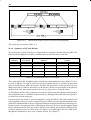
This book has been assembled from a number of sources. The authors of the chapters are as follows:
4
@
D
Q
W
g
h
o
t
7
{
;
|}~m€{
{
;
|}~mƒ‚
{
;
|}~m {
;
|}~mƒ‡
!#"%$&('*)+-,/.102+3
576#893): .;);:=<>!/ !#"%$&('*);+3,?.02+3
=93AB,?.02+-C !#"%$&('*)+-,/.102+3
EF=GH;<I:J ;!?KL8" EF$M NPO:<
RS8$TABNU0V+-
KL XY <I1Z[[5\] ^_=G#<`APababABcd)0e;!f" %$&('*);+3,?.02+-
KL XY <I1Z[ ;!f
KL XY <I1Z[[5SJi !j ^_(kjAmlJ+-Nn:
RS8pq:<I<`An!sr[:
KL XY <I1Z[i !#k/=6uAmlJ) <>!0
KL%RSJ^#!; ,_0`5R=%$&(XvH;<I<>:15R=8 pq:<I<`An!3r7:[5
"w3 x]AP;ABr=cb+-5=k/=6uAml)1 <>!0e !#"Ey($z:=NmlJ)
KL8"Ey($NPO:<
KL8"Ey($NPO:<
6f(w„<… l†An0
6f(w„<… l†An0
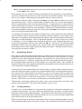
The editors would also like to thank all those who assisted with the preparation of the manuscript,
particularly Alan Pinder and Glenn Hill of the INMOS documentation group, who provided vital
support for the use of the document preparation system.
Work on this subject has been supported under various ESPRIT projects, in particular ‘Parallel
Universal Message-passing Architecture’ (PUMA, P2701), and more recently also under the
‘General Purpose MIMD’ (P5404) project. The assistance of the EC is gratefully acknowledged.
ˆ
Contents
Preface . . . . . . . . . . . . . . . . . . . . . . . . . . . . . . . . . . . . . . . . . . . . . . . . . .
v
1 Transputers and Routers: Components for Concurrent Machines .
1
1.1
1.2
1.3
1.4
1.5
1.6
1.7
Introduction . . . . . . . . . . . . . . . . . . . . . . . . . . . . . . . . . . . . . . . . . . . . . . . . . . .
Transputers . . . . . . . . . . . . . . . . . . . . . . . . . . . . . . . . . . . . . . . . . . . . . . . . . . . .
Routers . . . . . . . . . . . . . . . . . . . . . . . . . . . . . . . . . . . . . . . . . . . . . . . . . . . . . . .
Message Routing . . . . . . . . . . . . . . . . . . . . . . . . . . . . . . . . . . . . . . . . . . . . . . .
Addressing . . . . . . . . . . . . . . . . . . . . . . . . . . . . . . . . . . . . . . . . . . . . . . . . . . . .
Universal Routing . . . . . . . . . . . . . . . . . . . . . . . . . . . . . . . . . . . . . . . . . . . . . .
Conclusions . . . . . . . . . . . . . . . . . . . . . . . . . . . . . . . . . . . . . . . . . . . . . . . . . . .
1
1
2
6
9
12
14
2 The T9000 Communications Architecture . . . . . . . . . . . . . . . . . . . . .
15
2.1
2.2
2.3
2.4
2.5
2.6
2.7
2.8
Introduction . . . . . . . . . . . . . . . . . . . . . . . . . . . . . . . . . . . . . . . . . . . . . . . . . . .
The IMS T9000 . . . . . . . . . . . . . . . . . . . . . . . . . . . . . . . . . . . . . . . . . . . . . . . .
Instruction set basics and processes . . . . . . . . . . . . . . . . . . . . . . . . . . . . . . . . .
Implementation of Communications . . . . . . . . . . . . . . . . . . . . . . . . . . . . . . . .
Alternative input . . . . . . . . . . . . . . . . . . . . . . . . . . . . . . . . . . . . . . . . . . . . . . .
Shared channels and Resources . . . . . . . . . . . . . . . . . . . . . . . . . . . . . . . . . . . .
Use of resources . . . . . . . . . . . . . . . . . . . . . . . . . . . . . . . . . . . . . . . . . . . . . . . .
Conclusion . . . . . . . . . . . . . . . . . . . . . . . . . . . . . . . . . . . . . . . . . . . . . . . . . . . .
15
15
16
18
24
28
34
36
3 DS-Links and C104 Routers . . . . . . . . . . . . . . . . . . . . . . . . . . . . . . . . .
39
3.1
3.2
3.3
3.4
3.5
3.6
3.7
Introduction . . . . . . . . . . . . . . . . . . . . . . . . . . . . . . . . . . . . . . . . . . . . . . . . . . .
Using links between devices . . . . . . . . . . . . . . . . . . . . . . . . . . . . . . . . . . . . . .
Levels of link protocol . . . . . . . . . . . . . . . . . . . . . . . . . . . . . . . . . . . . . . . . . . .
Channel communication . . . . . . . . . . . . . . . . . . . . . . . . . . . . . . . . . . . . . . . . .
Errors on links . . . . . . . . . . . . . . . . . . . . . . . . . . . . . . . . . . . . . . . . . . . . . . . . .
Network communications: the IMS C104 . . . . . . . . . . . . . . . . . . . . . . . . . . . .
Conclusion . . . . . . . . . . . . . . . . . . . . . . . . . . . . . . . . . . . . . . . . . . . . . . . . . . . .
39
39
39
42
45
46
54
4 Connecting DS-Links . . . . . . . . . . . . . . . . . . . . . . . . . . . . . . . . . . . . . .
55
4.1
4.2
4.3
4.4
4.5
Introduction . . . . . . . . . . . . . . . . . . . . . . . . . . . . . . . . . . . . . . . . . . . . . . . . . . .
Signal properties of transputer links . . . . . . . . . . . . . . . . . . . . . . . . . . . . . . . .
PCB connections . . . . . . . . . . . . . . . . . . . . . . . . . . . . . . . . . . . . . . . . . . . . . . .
Cable connections . . . . . . . . . . . . . . . . . . . . . . . . . . . . . . . . . . . . . . . . . . . . . .
Error Rates . . . . . . . . . . . . . . . . . . . . . . . . . . . . . . . . . . . . . . . . . . . . . . . . . . . .
55
55
56
58
64
‰(Š
4.6
4.7
4.8
4.9
4.10
Optical interconnections . . . . . . . . . . . . . . . . . . . . . . . . . . . . . . . . . . . . . . . . .
Standards . . . . . . . . . . . . . . . . . . . . . . . . . . . . . . . . . . . . . . . . . . . . . . . . . . . . .
Conclusions . . . . . . . . . . . . . . . . . . . . . . . . . . . . . . . . . . . . . . . . . . . . . . . . . . .
References . . . . . . . . . . . . . . . . . . . . . . . . . . . . . . . . . . . . . . . . . . . . . . . . . . . .
Manufacturers and products referred to . . . . . . . . . . . . . . . . . . . . . . . . . . . . . .
65
67
68
69
70
5 Using Links for System Control . . . . . . . . . . . . . . . . . . . . . . . . . . . . . .
71
5.1
5.2
5.3
5.4
5.5
5.6
5.7
5.8
5.9
Introduction . . . . . . . . . . . . . . . . . . . . . . . . . . . . . . . . . . . . . . . . . . . . . . . . . . .
Control networks . . . . . . . . . . . . . . . . . . . . . . . . . . . . . . . . . . . . . . . . . . . . . . .
System initialization . . . . . . . . . . . . . . . . . . . . . . . . . . . . . . . . . . . . . . . . . . . .
Debugging . . . . . . . . . . . . . . . . . . . . . . . . . . . . . . . . . . . . . . . . . . . . . . . . . . . .
Errors . . . . . . . . . . . . . . . . . . . . . . . . . . . . . . . . . . . . . . . . . . . . . . . . . . . . . . . .
Embedded applications . . . . . . . . . . . . . . . . . . . . . . . . . . . . . . . . . . . . . . . . . .
Control system . . . . . . . . . . . . . . . . . . . . . . . . . . . . . . . . . . . . . . . . . . . . . . . . .
Commands . . . . . . . . . . . . . . . . . . . . . . . . . . . . . . . . . . . . . . . . . . . . . . . . . . . .
Conclusions . . . . . . . . . . . . . . . . . . . . . . . . . . . . . . . . . . . . . . . . . . . . . . . . . . .
71
73
75
78
79
81
81
83
84
6 Models of DS–Link Performance . . . . . . . . . . . . . . . . . . . . . . . . . . . .
85
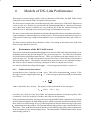
6.1
6.2
6.3
6.4
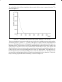
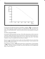
Performance of the DS–Link Protocol . . . . . . . . . . . . . . . . . . . . . . . . . . . . . . .
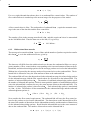
Bandwidth Effects of Latency . . . . . . . . . . . . . . . . . . . . . . . . . . . . . . . . . . . . .
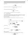
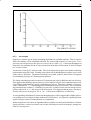
A model of Contention in a Single C104 . . . . . . . . . . . . . . . . . . . . . . . . . . . . .
Summary . . . . . . . . . . . . . . . . . . . . . . . . . . . . . . . . . . . . . . . . . . . . . . . . . . . . .
85
90
95
103
7 Performance of C104 Networks . . . . . . . . . . . . . . . . . . . . . . . . . . . . . .
105
7.1
7.2
7.3
7.4
7.5
7.6
7.7
7.8
The C104 switch . . . . . . . . . . . . . . . . . . . . . . . . . . . . . . . . . . . . . . . . . . . . . . .
Networks and Routing Algorithms . . . . . . . . . . . . . . . . . . . . . . . . . . . . . . . . .
The Networks Investigated . . . . . . . . . . . . . . . . . . . . . . . . . . . . . . . . . . . . . . .
The traffic patterns . . . . . . . . . . . . . . . . . . . . . . . . . . . . . . . . . . . . . . . . . . . . . .
Universal Routing . . . . . . . . . . . . . . . . . . . . . . . . . . . . . . . . . . . . . . . . . . . . . .
Results . . . . . . . . . . . . . . . . . . . . . . . . . . . . . . . . . . . . . . . . . . . . . . . . . . . . . . .
Performance Predictability . . . . . . . . . . . . . . . . . . . . . . . . . . . . . . . . . . . . . . .
Conclusions . . . . . . . . . . . . . . . . . . . . . . . . . . . . . . . . . . . . . . . . . . . . . . . . . . .
105
105
107
109
110
110
116
117
8 General Purpose Parallel Computers . . . . . . . . . . . . . . . . . . . . . . . . .
119
8.1
8.2
8.3
8.4
8.5
Introduction . . . . . . . . . . . . . . . . . . . . . . . . . . . . . . . . . . . . . . . . . . . . . . . . . . .
Universal message passing machines . . . . . . . . . . . . . . . . . . . . . . . . . . . . . . .
Networks for Universal message passing machines . . . . . . . . . . . . . . . . . . . .
Building Universal Parallel Computers from T9000s and C104s . . . . . . . . . .
Summary . . . . . . . . . . . . . . . . . . . . . . . . . . . . . . . . . . . . . . . . . . . . . . . . . . . . .
119
119
122
126
131
‹Œ Œ
9 The Implementation of Large Parallel Database Machines on T9000 and
C104 Networks . . . . . . . . . . . . . . . . . . . . . . . . . . . . . . . . . . . . . . . . . . . . . . 133
9.1
9.2
9.3
9.4
9.5
9.6
9.7
9.8
9.9
9.10
9.11
9.12
Database Machines . . . . . . . . . . . . . . . . . . . . . . . . . . . . . . . . . . . . . . . . . . . . .
Review of the T8 Design . . . . . . . . . . . . . . . . . . . . . . . . . . . . . . . . . . . . . . . . .
An Interconnection Strategy . . . . . . . . . . . . . . . . . . . . . . . . . . . . . . . . . . . . . .
Data Storage . . . . . . . . . . . . . . . . . . . . . . . . . . . . . . . . . . . . . . . . . . . . . . . . . . .
Interconnection Strategy . . . . . . . . . . . . . . . . . . . . . . . . . . . . . . . . . . . . . . . . .
Relational Processing . . . . . . . . . . . . . . . . . . . . . . . . . . . . . . . . . . . . . . . . . . . .
Referential Integrity Processing . . . . . . . . . . . . . . . . . . . . . . . . . . . . . . . . . . . .
Concurrency Management . . . . . . . . . . . . . . . . . . . . . . . . . . . . . . . . . . . . . . . .
Complex Data Types . . . . . . . . . . . . . . . . . . . . . . . . . . . . . . . . . . . . . . . . . . . .
Recovery . . . . . . . . . . . . . . . . . . . . . . . . . . . . . . . . . . . . . . . . . . . . . . . . . . . . .
Resource Allocation and Scalability . . . . . . . . . . . . . . . . . . . . . . . . . . . . . . . .
Conclusions . . . . . . . . . . . . . . . . . . . . . . . . . . . . . . . . . . . . . . . . . . . . . . . . . . .
133
134
136
137
139
140
141
142
145
146
146
148
10 A Generic Architecture for ATM Systems . . . . . . . . . . . . . . . . . . . . .
151
10.1
10.2
10.3
10.4
10.5
Introduction . . . . . . . . . . . . . . . . . . . . . . . . . . . . . . . . . . . . . . . . . . . . . . . . . . .
An Introduction to Asynchronous Transfer Mode . . . . . . . . . . . . . . . . . . . . . .
ATM Systems . . . . . . . . . . . . . . . . . . . . . . . . . . . . . . . . . . . . . . . . . . . . . . . . . .
Mapping ATM onto DS–Links . . . . . . . . . . . . . . . . . . . . . . . . . . . . . . . . . . . .
Conclusions . . . . . . . . . . . . . . . . . . . . . . . . . . . . . . . . . . . . . . . . . . . . . . . . . . .
151
152
162
177
181
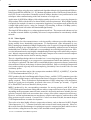
11 An Enabling Infrastructure for a Distributed Multimedia Industry
183
11.1
11.2
11.3
11.4
11.5
11.6
11.7
11.8
11.9
11.10
Introduction . . . . . . . . . . . . . . . . . . . . . . . . . . . . . . . . . . . . . . . . . . . . . . . . . . .
Network Requirements for Multimedia . . . . . . . . . . . . . . . . . . . . . . . . . . . . . .
Integration and Scaling . . . . . . . . . . . . . . . . . . . . . . . . . . . . . . . . . . . . . . . . . .
Directions in networking technology . . . . . . . . . . . . . . . . . . . . . . . . . . . . . . . .
Convergence of Applications, Communications and Parallel Processing . . . .
A Multimedia Industry – the Need for Standard Interfaces . . . . . . . . . . . . . . .
Outline of a Multimedia Architecture . . . . . . . . . . . . . . . . . . . . . . . . . . . . . . .
Levels of conformance . . . . . . . . . . . . . . . . . . . . . . . . . . . . . . . . . . . . . . . . . . .
Building stations from components . . . . . . . . . . . . . . . . . . . . . . . . . . . . . . . . .
Mapping the Architecture onto Transputer Technology . . . . . . . . . . . . . . . . .
183
183
186
186
187
188
189
194
195
196
Appendices:
A New link cable connector . . . . . . . . . . . . . . . . . . . . . . . . . . . . . . . . . . .
201
B Link waveforms . . . . . . . . . . . . . . . . . . . . . . . . . . . . . . . . . . . . . . . . . . .
203
C DS–Link Electrical specification . . . . . . . . . . . . . . . . . . . . . . . . . . . . .
205
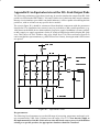
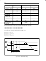
D An Equivalent circuit for DS–Link Output Pads . . . . . . . . . . . . . . . .
209
1
1
1.1
Transputers and Routers:
Components for Concurrent
Machines
Introduction
This chapter describes an architecture for concurrent machines constructed from two types of
component: ‘transputers’ and ‘routers’. In subsequent chapters we consider the details of these
two components, and show the architecture can be adapted to include other types of component.
A transputer is a complete microcomputer integrated in a single VLSI chip. Each transputer has
a number of communication links, allowing transputers to be interconnected to form concurrent
processing systems. The transputer instruction set contains instructions to send and receive messages through these links, minimizing delays in inter-transputer communication. Transputers can
be directly connected to form specialised networks, or can be interconnected via routing chips.
Routing chips are VLSI building blocks for interconnection networks: they can support systemwide message routing at high throughput and low delay.
1.2
Transputers
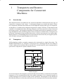
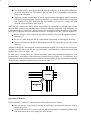
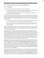
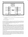
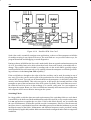
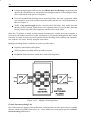
VLSI technology enables a complete computer to be constructed on a single silicon chip. The
INMOS T800 transputer [1], integrates a central processor, a floating point unit, four kilobytes
of static random access memory plus an interface for external memory, and a communications
system onto a chip about 1 square centimetre in area.
!#"%$'&
T800 Transputer
As a microcomputer, the transputer is unusual in that it has the ability to communicate with other
transputers via its communication links; this enables transputers to be connected together to
construct multiprocessor systems to tackle specific problems. The transputer is also unusual in
that it has the ability to execute many software processes, sharing its time between them automati-
2
cally, to create new processes rapidly, and to perform communication between processes within
a transputer and between processes in different transputers. All of these capabilities are integrated into the hardware of the transputer, and are very efficient. This is discussed in more detail
in chapter 2.
The use of transputers for parallel programming has been greatly simplified by the development
of the occam programming language [2]. The occam language allows an application to be expressed as a collection of concurrent processes which communicate via channels. Each channel
is a point-to-point connection between two processes; one process always inputs from the channel
and the other always outputs to it. Communication is synchronised; the first process ready to
communicate waits until the second is also ready, then the data is copied from the outputting processes to the inputting process and both processes continue.
Each transputer has a process scheduler which allows it to share its time between a number of
processes. Communication between processes on the same transputer is performed using the local memory; communication between processes on different transputers is performed using a link
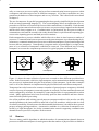
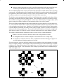
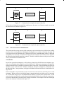
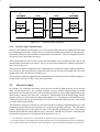
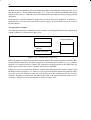
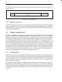
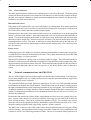
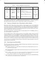
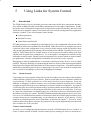
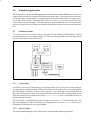
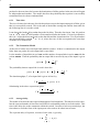
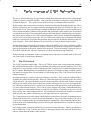
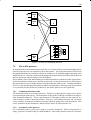
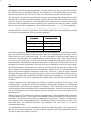
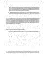
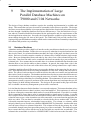
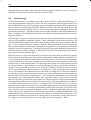
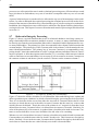
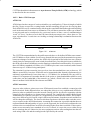
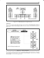
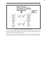
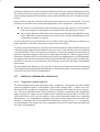
between the two transputers. Consequently, a program can be executed either by a single transputer or by a collection of transputers connected in a network. Three different ways of using
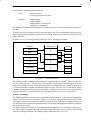
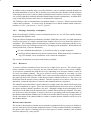
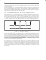
transputers to execute the component processes of a typical program are shown below.
1 transputer
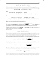
Figure 1.1
3 transputers
5 transputers
Allocations of processes to processors
Figure 1.1 shows the same collection of processes executed on three different specialised networks. In the first network, which is a single transputer, each communication channel connecting
two processes is implemented using the local memory of the transputer. In the other examples
some or all of the channels are implemented by physical links between different transputers.
Transputers have also been used to construct a number of general purpose computers, which all
consist of an array of transputers connected together in a network. In some machines the network
can be configured by software, for example by connecting the links via a programmable crossbar
switch. Many applications have been successfully ported to these machines and have demonstrated efficient parallel processing.
One of the problems with existing general purpose transputer machines is the need to carefully
match algorithms to the interconnection networks of specific machines, which results in a lack
of software portability. It has become clear that a standard architecture is needed for these general
purpose message-passing machines. An attractive candidate is a collection of transputers connected by a high throughput, low delay communication network supporting communication
channels between processes anywhere in the network.
1.3
Routers
There are many parallel algorithms in which the number of communication channels between
processes on different transputers is much greater than the number of physical links available to
3
connect the transputers. In some of these algorithms, a process executed on one transputer must
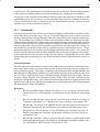
communicate with processes on a large number of other transputers. These requirements for system-wide communication between processes can be met by:
(
(
new transputers including hardware to multiplex many ‘virtual links’ along a single physical link (see chapter 2)
new VLSI message-routing chips (routers) which can be used to construct efficient communication networks
This new communications architecture allows communication channels to be established between any two processes, regardless of where they are physically located in the system. This simplifies programming because processes can be allocated to transputers to optimize performance
after the program has been written. For general purpose message-passing computers, a further
benefit is that processes can be allocated to transputers by a compiler, which effectively removes
configuration details from the program, thereby enhancing portability.
)+*
/021 53 46
)
)+*
/021 3546
,
/021 3546
-7/021 3546
-78
/021 3546
8.9
)+*
/021 3546
-.,
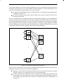
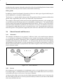
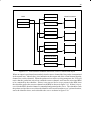
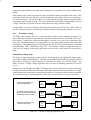
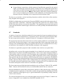
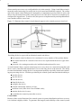
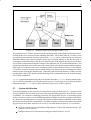
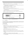
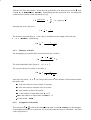
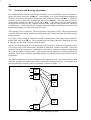
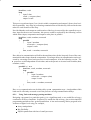
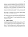
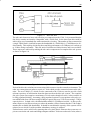
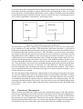
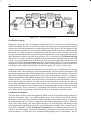
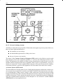
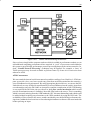
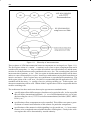
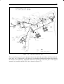
Figure 1.2 Network constructed from routers
The use of two separate chips, one to perform computing (the transputer) and one to perform communication (the router) has several practical advantages:
(
(
Transputers can be directly connected without routers in systems which do not require
message routing, so avoiding the silicon cost and routing delays.
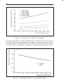
It allows routers to have many links (e.g.32) which in turn allows large networks to be
constructed from a small number of routers, minimizing the delay through the network.
For example, 48 such routers can connect 512 terminals with only 3 routing delays, as
in figure 1.2.
4
:
:
It avoids the need for messages to flow through the transputer, reducing the total throughput of the chip interface. This reduces the pin count, power consumption and package
costs of the transputer.
It supports scalable architectures in which communication throughput must be balanced
with processing throughput. In such architectures, it is known that overall communication capacity must grow faster than the total number of processors - a larger machine
must have proportionately more routers.
Since the new architecture allows all the virtual links of a transputer to pass through a single
physical link, system-wide communication can be provided by connecting each transputer to a
routing network via a single link. The provision of several links on transputers allows each transputer to be connected to several different networks. Examples of the use of this technique are:
:
:
The use of two (or more) identical networks in parallel to increase throughput and fault–
tolerance [7]
The use of a main network and an (independent) monitoring and debugging network
:
The use of a main network and an independent network for input and output (or for access
to discs)
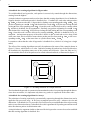
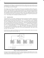
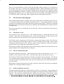
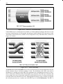
Another technique for increasing the communications throughput is to construct the network using two (or more) links in parallel for each connection. An example of a 2-dimensional network
of this kind is shown in figure 1.4.
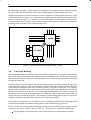
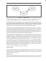
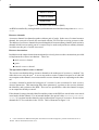
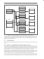
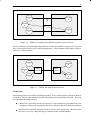
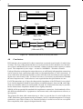
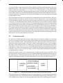
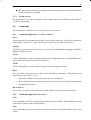
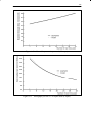
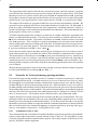
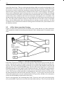
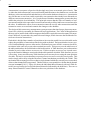
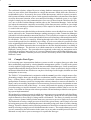
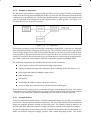
In some cases, it is convenient to construct a network from routers and attach transputers to its
terminal links. An example is the multi-stage network shown in figure 1.2. An alternative is to
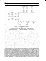
construct a network such as a hypercube or an array from a number of nodes, each node consisting
of one or more transputers and a router as shown in figure 1.4.
FG2B C5E<
;=<%>?@ABDC!E<
Figure 1.3 Node combining a transputer and a router
Operation of Routers
Each router has a number of communication links and operates as follows:
:
:
It uses the header of each packet arriving on each link to determine the link to be used to
output the packet;
It arbitrates between two (or more) packets which must both be output through the same
link, and causes them to be output one after another;
5
H
It starts to output each packet as early as possible (immediately after the output link is determined, provided that the output link is not already in use for another packet).
The overall throughput of the router is determined by the number of links which can be operating
concurrently. An important benefit of employing serial links for packet routing is that it is simple
to implement a full crossbar switch in VLSI, even for a large number of links. Use of a full crossbar allows packets to be passing through all of the links at the same time.
The ability to start outputting a packet whilst it is still being input can significantly reduce delay,
especially in networks which are lightly loaded. This technique is known as wormhole routing.
In wormhole routing, the delay through the switch can be minimized by keeping headers short
and by using fast, simple, hardware to determine the link to be used for output.
The use of simple routing hardware allows this capability to be provided for every link in the router. This avoids the need to share it between many links which would increase delay in the event
of several packets arriving at once. Equally, it is desirable to avoid the need for the large number
of packet buffers commonly provided in some packet routing systems (in which each packet is
input to a buffer before output starts). The use of small buffers together with simple routing hardware allows a single VLSI chip to provide efficient routing between a large number of links.
The simple communications architecture allows a wide variety of implementations:
H
CMOS VLSI can be used to construct routers with a large number of links;
H
H
It is straightforward to combine transputers and small routers on a single chip;
It is possible to construct routers in ECL or Gallium Arsenide technology to support extremely high speed implementations of the link.
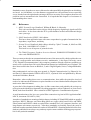
For some purposes, it may be useful to combine a router together with each transputer in a single
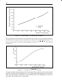
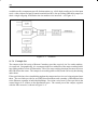
chip (or a single package). One example is the construction of a two dimensional array of simple
transputers for image processing (for this application, no off-chip memory is needed, and most
communication is local). The architecture of the routing system makes such a combination possible, as in figure 1.4.
Figure 1.4 Two dimensional array of nodes
6
1.4
Message Routing
1.4.1
Avoiding Deadlock
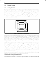
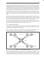
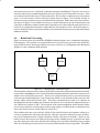
The purpose of a communications network is to support efficient and reliable communication between processes. Consequently, an essential property of a communications network is that it
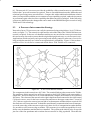
should not deadlock, i.e. arrive in a state where further progress is impossible. However, deadlock can occur in most networks unless the routing algorithm is designed to prevent it. For example, consider the square of four nodes shown in figure 1.5. Suppose that every node attempts to
send a packet to the opposite corner at the same time, and that the routing algorithm routes packets
in a clockwise direction. Then each link will become ‘busy’ sending a packet to the adjacent corner and the network will deadlock.
Figure 1.5 Deadlock in a simple network
It is important to understand that deadlock is a property of the network topology and the routing
algorithm used; it can also arise with buffered packet routing. In the above example, a single
packet buffer at each node is sufficient to remove the deadlock but, in general, the number of
packet buffers needed to eliminate deadlock depends on the network topology, the routing algorithm and the applications program. This is clearly not a satisfactory basis for a general purpose
routing system.
All of the above problems can be avoided by choosing networks for which deadlock-free wormhole routing algorithms exist. In such networks, buffers are employed only to smooth the flow
of data through the network and to reduce congestion; often a buffer of size much less than the
length of a packet is sufficient for this purpose. Most important of all, the buffering needed is
not dependent on the network size or the applications program. It is possible to construct a single
universal router which can be used for networks of arbitrary size and for programs of arbitrary
complexity. An essential property of such a router is that, like a transputer, it can communicate
on all of its links concurrently.
It turns out that many regular networks constructed from such routers have deadlock free routing
algorithms. Important examples are trees, hypercubes and grids.
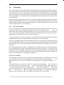
A deadlock free routing algorithm for Trees
A tree consists of a collection of nodes with a single external link from the root. Assume that
7
two trees1 IKJ with root link LMJ and I.N with root link LON are both deadlock free; they will always
perform internal communication without deadlock, and will accept and transmit packets along
the root link without deadlock.
A new tree is formed by connecting the root links LPJ and L#N to a new root node Q ; a further link
L on this node is the root link of the newly constructed tree I .
Any packet arriving at Q along LPJ is routed either to LON or to L . If it is routed to LON , it will be consumed by I.N , because IN is deadlock free. If it is routed to L , it will eventually be consumed by
the environment. By symmetry, packets arriving along LPJ will also be consumed. A packet arriving along L will be routed to either IKJ or IN ; in either case it will be consumed because both IKJ and
I.N are deadlock free.
It remains to show that a tree with only one node is deadlock free; this is true because the node
can send and receive packets concurrently along its single (root) link.
RTS
RUS
RTS
RUS
Figure 1.6 Hypercube constructed from 2N+2 Nodes
1. Note that this construction can easily be generalized from binary to n-ary trees.
8
A deadlock free routing algorithm for Hypercubes
To avoid deadlock in a hypercube, each packet is successively routed through the dimensions,
starting from the highest.
A simple inductive argument can be used to show that this routing algorithm is free of deadlocks.
Suppose
the order-V hypercube is deadlock free. Combine two such orderV hypercubes
WYX and W[Z that
Y
W
X
W[Z
to form an order-(V +1)WYhypercube
by linking corresponding
nodes of and . Any
X
W
Z
packet originating at a node \ in
andW[destined
for a node in
will first travel along the link
Z
corresponding node in ; from this node it will be delivered by routing within
W joining
W Z
Z and \thisto isthedeadlock
\
free
by
assumption.
Similarly,
any
packet
originating
at
a
node
in
W X will first travel along the link joining \ to the corresponding node
andWYdestined
for a node in
X
WYX and this is deadlock free by asin ; from this node it will be delivered by routing within
sumption. An important property of the node is that it is able to send and receive
a link
X in WYX toalong
at the same time;Z thisW isZ needed to ensure that a packet can flow from
node
the
corre]
X
Z
sponding node ] in
at the same time as a packet flows into ] from ] .
It remains to show that the order-0 hypercube is deadlock free (which it is, being just a single
node)!
The effect of the routing algorithm can easily be understood in terms of the example shown in
figure 1.5 above, which shows a 2–cube. Instead of routing all packets in a clockwise direction,
the deadlock-free algorithm routes two of the packets anti-clockwise. Since the links are bi–
directional this allows all of the packets to be routed without deadlock, as illustrated in figure 1.7.
Figure 1.7 Avoiding deadlock in a simple network
The fact that the hypercube is symmetrical means that the order of sequencing through the dimensions does not matter; it is important only that every packet is sequenced in the same order.
A deadlock free routing algorithm for Arrays
The technique of routing a packet by systematically sequencing through the dimensions can be
applied to any processor array. In fact, any rectangular processor array - whatever its size and
dimension - is deadlock free! To prove this it is first necessary to establish that a line of processing
nodes (a one-dimensional array) is deadlock free; this is guaranteed if a packet generated at a node
takes the shortest path to its destination node.
A simple inductive argument similar to that used for the hypercube can now be used to establish
that this routing algorithm is deadlock free.
9
1.5
Addressing
Every packet must carry with it the address of its destination; this might be the address of a transputer, or the address of one of a number of virtual channels forming input channels to a transputer.
As a packet arrives at a router, the destination address must be inspected before the outgoing link
can be determined; the delay through the router is therefore proportional to the address length.
Further, the address must itself be transmitted through the network and therefore consumes network bandwidth.
It is therefore important that this address be as short as possible, both to optimize network latency
and network bandwidth. However, it is also important that the destination link can be derived
from the address quickly and with minimal hardware. An addressing system which meets both
of these requirements is interval labelling.
1.5.1
Interval Labelling
An interval labelling scheme [6] assigns a distinct label to each transputer in a network. For simplicity, the labels for an ^ transputer network can be numbers in the range [0,1, . . . ,^ –1]. At
each router in the network, each output link has one or more associated intervals, where an interval is a set of consecutive labels. The intervals associated with the links on a router are non-overlapping and every label will occur in exactly one interval.
As a packet arrives at a router, the address is examined to determine which interval contains a
matching label; the packet is then forwarded along the associated output link.
The interval labelling scheme requires minimal hardware; at most a pair of comparators for each
of the outgoing links. It is also very fast, since the output link can be determined, once the address
has been input, after only a single comparison delay provided all the comparisons are done concurrently.
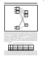
There remains the question of how to assign labels to an arbitrary network. The following examples give labelings for networks constructed from nodes as shown in figure 1.3. Intervals are represented with the notation [_ ,` ), which means the set of labels greater than or equal to _ and less
than ` ; note however that the comparisons are performed modulo the total number of labels, and
intervals are permitted to ‘wrap around’ through zero.
Trees can be labelled
The transputers in a binary tree2 with ^ nodes are labelled as follows. Suppose there are a nodes
to the left of the root node. Then the transputers to the left of the root are numbered 0, . . . , a –1;
the transputer of the root node is labelled a ; the transputers to the right are labelled a +1,. . .
,^cb 1,
Any node d in the tree is itself the root node of a subtree e with nodes f5g , . . . , f%h . The interval
associated with the left link of d is [f g , . . . , d ); that associated with the right link is [d +1,
. . .,f h +1); that associated with the root link is [f h +1, . . . ,f g ). The interval [f h +1, . . . ,f g ) consists
of all of the labels in the tree apart from those in e ; numerically it consists of the two intervals
[f%h +1, . . . ,^ +1) and [0, . . . ,f!g ). An example is shown in figure 1.8. This shows the labels assigned to each node, and the intervals assigned to the links of two of the nodes.
2. This construction can easily be generalized from binary to general trees, as illustrated in figure 1.8.
10
[0,9)
8
9
[11,14)
[10,11)
3
9
[0,10) U
[11,14)
0
1
4
5
2
6
7
10
11
12
10
13
Figure 1.8 A Tree with Interval Labelling
Hypercubes can be labelled
The labelling of the hypercube follows the construction given for the deadlock free routing algorithm. In combining the two order-i hypercubes jYk and j[l , the transputers in jYk are labelled
k
0, . . . , 2 m – 1 and those in j[l are labelled 2 m , . . . ,2 mn – 1. The link from each node oKk in jYk
k
to the corresponding node o7l in j[l is labelled with the interval [2 m , . . . ,2 m'n ) at oKk , and with
[0, . . . ,2 m ) at o7l . This inductively constructs a hypercube together with the deadlock-free routing algorithm described above.
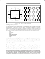
Arrays can be labelled
The labelling for an array follows the construction of the deadlock free routing algorithm. An
i -dimensional array is composed of p arrays of dimension i –1, with p corresponding nodes
(one from each i –1 dimensional array) joined to form a line. If each of the i –1 dimensional arrays has q nodes, the nodes in the i –1 dimensional arrays are numbered 0, . . ., q –1; q , . . ., 2q –1;
. . .; (p –1)q , . . ., prq –1. On every line the link joining the s5tvu node to the (s +1) t u node is labelled
[s q , . . ., pwq ) and the link to the (s –1) tvu node is labelled [0, . . ., (s –1)q ). This inductively labels
an array to route packets according to the deadlock free algorithm described above. An example
is shown in figure 1.9. This shows the labels assigned to each node, and the intervals assigned
to the links of one of the nodes.
11
[0,8)
[8,9)
9
0
1
2
3
4
5
6
7
8
9
10
11
12
13
14
15
[10,12)
[12,16)
Figure 1.9 An Array with Interval Labelling
Labelling arbitrary networks
The above labelings provide optimal routing, so that each packet takes one of the shortest paths
to its destination. It can easily be shown [6] that any network can be labelled so as to provide
deadlock free routing; it is only necessary to construct a spanning tree and label it as described
above. This may produce a non-optimal routing which cannot exploit all of the links present in
the network as a whole. Optimal labelings are known for all of the networks shown below:
trees
hypercubes
arrays
multi-stage networks
butterfly networks
rings3
In high performance embedded applications (or in reconfigurable computers) specialised networks are often used to minimize interconnect costs or to avoid the need for message routing.
In these systems, a non-optimal labelling can be used to provide low-speed system-wide communications such as would be needed for system configuration and monitoring.
1.5.2
Header Deletion
The main disadvantages of the interval labelling system are that it does not permit arbitrary routes
through a network, and it does not allow a message to be routed through a series of networks.
These problems can be overcome by a simple extension: header deletion. Any link of a router
can be set to delete the header of every packet which passes out through it; the result is that the
data immediately following becomes the new header as the packet enters the next node.
Header deletion can be used to minimize delays in the routing network. To do this, an initial header is used to route the packet to a destination transputer; this header is deleted as it leaves the final
router and enters the transputer. A second header is then used to identify the virtual link within
3. Note that the optimal labelling of a ring requires that one of the connections be duplicated in order to avoid
deadlock.
12
the destination transputer. As the number of transputers is normally much less than the number
of virtual links, the initial header can be short, minimizing the delay through each router.
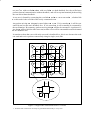
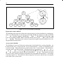
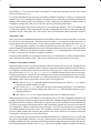
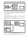
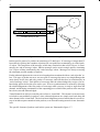
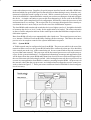
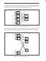
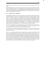
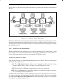
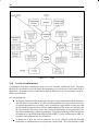
Another important use of header deletion is in the construction of hierarchical networks. In the
2-dimensional array of figure 1.4, each transputer could be replaced with a local network of transputers as shown in figure 1.10. Headers are deleted as packets leave or enter a local network.
A single header can be used to route a packet within a local network, whilst three headers are
needed to route a packet via the 2-dimensional array.
xzy|{~}€T
xzy|{~}€T
Figure 1.10 Local network of transputers and a router
1.6
Universal Routing
The routing algorithms described so far provide efficient deadlock free communications and allow a wide range of networks to be constructed from a standard router. Packets are delivered at
high speed and with low latency provided that there are no collisions between packets travelling
through the same link.
Unfortunately, for general purpose concurrent computers, this may not be enough. In any sparse
communication network, some communication patterns cannot be realized without collisions.
Such collisions within the network can reduce system performance drastically. For example,
some parallel algorithms require that all messages from one phase of a computation are delivered
before the next phase starts; the late arrival of a single message delays all of the processors. In
the absence of any bound on message latency it is difficult - and in many cases impossible - to
design efficient concurrent programs. The problem of constructing general purpose concurrent
computers therefore depends on the answer to the following question:
Is it possible to design a universal routing system: a realizable network and a routing algorithm
which can implement all communication patterns with bounded message latency?
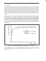
In fact, a universal routing system allowing the construction of scalable general purpose parallel
computers was discovered by Valiant in 1980 [3]. This meets two important requirements:
‚
The throughput of the network increases proportionately with the number of nodes.
13
ƒ
The delay through the network increases only slowly with the number of nodes (proportional to „O…‡† (ˆ2‰ for ˆ nodes).
Notice that the aim is to maximize capacity and minimize delay under heavy load conditions a parallel communications network is a vital component of a parallel computer. This is not the
same as, for example, minimizing delay through an otherwise empty network.
A ˆ -node hypercube has a delay of proportional to „O…‡† (ˆ ) (written Š („O…‹† (ˆ ))) if there are no collisions between packets. This is an unreasonable assumption, however, as all of the transputers
will be communicating via the network simultaneously. An important case of communication
is that of performing a permutation in which every transputer simultaneously transmits a message
and no two messages head for the same destination. Valiant’s proof [4] demonstrates constructively that permutation routing is possible in a time proportional to „O…‹† (ˆ ) on a sparseˆ -node network even at high communication load.
To eliminate the network hot-spots which commonly arise when packets from many different
sources collide at a link in a sparse network, two phase routing is employed. Every packet is first
dispatched to a randomly chosen intermediate destination; from the intermediate destination it
continues to its final destination. This is a distributed algorithm - it does not require any central
co-ordination - so it is straightforward to implement and scales easily. Randomization does not,
in fact, strictly guarantee a delivery time which is Š („O…‹† (ˆ )) - but it gives it a sufficiently high
probability to achieve the universality result. The processors will occasionally be held up for a
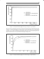
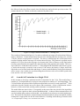
late message, but not often enough to noticeably affect performance. Simulated results of universal routing are presented in chapter 7.
1.6.1
Randomizing Headers
How is the two-phase algorithm implemented? As a packet enters a randomizing network, it must
be supplied with a new, random, header; this header will be used to route the packet to a router
which will serve as the intermediate destination. Any input link of a router can be set to randomize packets as they arrive. Whenever a packet starts to arrive along such a link, the link first generates a random number and behaves as if this number were the packet header. The remainder of
the packet follows the newly supplied random header through the network until the header reaches the intermediate (random) destination.
At this point, the first (randomizing) phase of the routing is complete and the random header is
removed to allow the header to progress to its final destination in the second (destination) phase.
The removal of the random header is performed by a portal in each router which recognizes the
random header associated with the router. The portal deletes the random header with the result
that the original header is at the front of the packet, as it was when the packet first entered the
network. This header is now used to route the packet to its final destination.
Unfortunately, performing routing in two phases in the same network makes the paths of the
packets more complicated. The result is that deadlock can now occur.
1.6.2
Avoiding Deadlock
A simple way to avoid deadlock is to ensure that the two phases of the packet transmission use
completely separate links. The node numbers are partitioned into two halves: one half contains
the numbers used for the randomizing phase. The numbers in the other half are used for the destination phase. Similarly the links are partitioned into two sets: one set is used in the randomizing
phase and the other set in the destination phase.
Effectively this scheme provides two separate networks, one for the randomizing phase, and one
for the destination phase, with only one set of routers. The combination of the two networks will
14
be deadlock free if both of the networks are deadlock free. The simplest arrangement is to make
the randomizing network have the same structure as the destination network - and to make both
employ one of the known deadlock free routing algorithms.
Universal routing can be applied to a wide variety of networks including hypercubes and arrays
[5].
1.7
Conclusions
Concurrent machines can be constructed from two components: transputers and routers. Transputers can be connected via their links to form dedicated processing systems in which communication takes place only between directly connected transputers. They can also be connected
via routers allowing system-wide communication.
The provision of system-wide inter-process communication simplifies the design and programming of concurrent machines. It allows processes to be allocated to transputers after a program
is written in order to optimize performance or minimize cost. It ensures that programs will be
portable between different machines, although their performance will vary depending on the capabilities of the specific communications network used.
The communications architecture allows a wide variety of implementations. VLSI routers can
provide routing between a large number of links, minimizing network delays. Very fast routers
with fewer links can be constructed using high-speed technology. Transputers and routers can
be combined on VLSI chips to provide network nodes.
Transputers and routers can be used to build machines in which a balance is maintained between
communication throughput and processing throughput. Universal routing can be used to achieve
bounded communication delay, and fast process scheduling within the transputers allows this
communication delay to be hidden by a small amount of excess parallelism. An immediate possibility is the development of a standard architecture for scalable general purpose concurrent computers, as discussed in chapter 8.
References
[1]
M. Homewood, D. May, D. Shepherd, The IMS T800 Transputer
IEEE Micro 7 no. 5, October 1987
[2]
INMOS Limited, occam2 reference manual, Prentice Hall 1988
[3]
L.G. Valiant, A scheme for fast parallel communication
SIAM J. on Computing 11 (1982) pp. 350–361
[4]
L.G. Valiant, General Purpose Parallel Architectures,
TR–07–89, Aiken Computation Laboratory, Harvard University
[5]
L.G. Valiant, G.J. Brebner, Universal Schemes for Parallel Communication
ACM STOC (1981) pp. 263–277
[6]
J. van Leeuwen, R.B. Tan Interval Routing
The Computer Journal 30 no. 4 pp. 298–307 1987
[7]
P. Thompson, Globally Connected Fault–Tolerant Systems
in Transputer and occam Research: New Directions, J. Kerridge (Ed)
IOS Press 1993
15
2
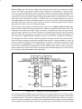
2.1
The T9000 Communications
Architecture
Introduction
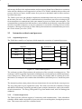
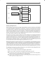
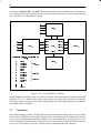
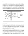
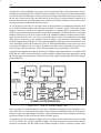
This chapter describes the communications capabilities implemented in the IMS T9000 transputer, and supported by the IMS C104 packet router, which is discussed in chapter 3. The T9000
retains the point-to-point synchronised message passing model implemented in first generation
of transputers but extends it in two significant ways. The most important innovation of the T9000
is the virtualization of external communication. This allows any number of virtual links to be
established over a single hardware link between two directly connected T9000s, and for virtual
links to be established between T9000s connected by a routing network constructed from C104
routers. A second important innovation is the introduction of a many-one communication mechanism, the resource. This provides, amongst other things, an efficient distributed implementation
of servers.
2.2
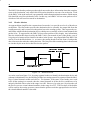
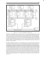
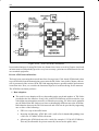
The IMS T9000
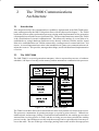
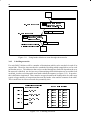
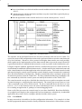
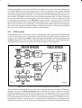
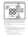
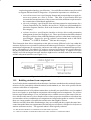
The IMS T9000 is a second–generation transputer; it has a superscalar processor, a hardware
scheduler, 16K bytes of on-chip cache memory, and an autonomous communications processor.
E'(+#+#E ; <
=>//4+#+
? (@"A
=>//4+#+
? (@"A<
7 $:9
8
+;%<'
5 ('<6<
I +J"4
I %K< '(+
L M+
B DC
.
F2 "G.E
5 6(<%
E'(+#+H
#)*(#"$
!(+,"--.'#"- (/1023"4
5 ('%6(
!#"$%&('(
Figure 2.1
NK@3"APOQ
The IMS T9000 Transputer
The T9000’s scheduler allows the creation and execution of any number of concurrent processes.
The processes communicate by passing messages over point-to-point channels. Channels are
unidirectional, and message passing is synchronised and unbuffered; the sending process must
wait until the receiving process is ready, and the receiving process must wait until the sending
process is ready. Once both processes are ready the message can be copied directly from one process to the other. The use of this type of message passing removes the need for message queues
16
and message buffers in the implementation, and prevents accidental loss of data due to variations
in the order in which processes happen to be executed. The T9000’s scheduler also provides each
process with its own timer, and the means for a process to deschedule until its timer reaches a
specified alarm time.
The T9000’s processor and scheduler implement communication between processes executing
on the same processor. The T9000’s communication system allows processes executing on different transputers to communicate in the same manner as processes on the same transputer. The
communication system has four link interfaces, each of which may be directly connected to a link
interface of another transputer, or may be connected via a network of routing devices to other
transputers. Messages are passed over these links by the autonomous communications processor,
the virtual channel processor (VCP).
2.3
Instruction set basics and processes
2.3.1
Sequential processes
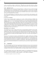
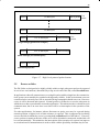
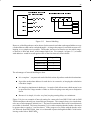
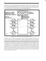
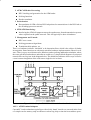
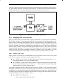
The T9000 has a small set of registers which support the execution of sequential processes:
Registers
Workspaces
FAreg
Areg
FBreg
Breg
FCreg
Creg
Program
Workspace
Next Instruction
Figure 2.2
IMS T9000 Registers
The workspace pointer (Wptr) points to the workspace of the currently executing process. This
workspace, which is typically organized as a falling stack, contains the local variables and temporaries of the process. When a process is not executing, for example while it is waiting for a communication, its workspace also contains other information, such as the process’ instruction pointer.
The instruction pointer (Iptr) points at the next instruction to be executed by the current process.
The Areg, Breg and Creg are organized as stack. The stack is used for the evaluation of integer
and address calculations, and as the operands of more complex instructions, such as the communication instructions. The FAreg, FBreg and FCreg form another stack, used for floating point
arithmetic.
2.3.2
Concurrent processes
The T9000 provides efficient support of concurrency and communication. It has a hardware
scheduler which enables any number of processes to be executed together, sharing the processor
time. This removes the need for a software kernel.
17
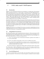
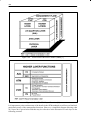
At any time, a concurrent process may be:
active
being executed
on a list waiting for execution
inactive
ready to input
ready to output
waiting until a specified time
waiting for a semaphore
The T9000’s scheduler operates in such a way that inactive processes do not consume any processor time.
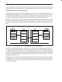
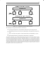
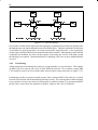
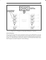
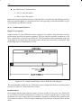
The active processes waiting to be executed are held on a list. This is a linked list of process workspaces, implemented using two registers, one of which points to the first process on the list, the
other to the last.
In figure 2.3, S is executing, and P, Q and R are active, awaiting execution.
Workspaces
Registers
Front
Program
P
Back
Q
A
B
R
C
S
Workspace
Next Instruction
Figure 2.3
Active processes
The T9000 provides a number of instructions to support the process model. These include start
process, and end process. The start process instruction creates a new concurrent process by adding a new workspace to the end of the scheduling list, enabling the new concurrent process to
be executed together with the ones already being executed. The end process instruction allows
a number of concurrent processes to join together, so that a successor process is executed when,
and only when, all of its predecessors have terminated with an end process instruction.
Priority scheduling
The T9000 scheduler is actually more complex than described above. It provides two scheduling
queues, one for each of two priorities. Whenever a process of high priority (priority 0) is able
to proceed, it will do so in preference to a low priority (priority 1) process. If a high priority process becomes active whilst a low priority process is executing, the high priority process preempts
the low priority process.
To identify a process entirely, it is necessary to identify both the process’ workspace and its priority. These can be encoded in a single word by or-ing the priority of the process into the bottom
bit of the workspace address; the resulting value is known as the process id.
18
2.4
Implementation of Communications
The T9000 provides a number of instructions which implement communication over channels.
These instructions use the address of the channel to determine whether the channel is internal or
is a virtual channel. This means that the same instruction sequence can be used, allowing a process to be written and compiled without knowledge of where its channels are connected.
Since channels are distinct objects from the processes which communicate over them, they serve
to hide the internal structure of such processes from each other. A process which interacts with
others only via channels thus has a very clean and simple interface, which facilitates the application of structured programming principles.
Before a channel can be used it must be allocated and initialized. The details depend on whether
the channel is to connect two processes on the same transputer, or two processes on different
transputers.
2.4.1
Variable length input and output
The variable input message (vin), variable output message (vout) and load count instructions provide the basic message passing mechanism of the T9000. They convey a message and its length,
from an sending process to an receiving process. The receiver specifies the maximum length of
message that it is prepared to receive, and the sender the actual length of the message to be sent.
If the actual length is longer than the receiver is prepared to receive than an error is signalled.
A sending process performs an output by loading the evaluation stack with a pointer to the message, the length of the message and the address of the channel. It then executes a vout instruction.
A receiving process performs an input by loading the evaluation stack with a pointer to the variable, the maximum length of message and the address of the channel. It then executes a vin
instruction followed by a load count instruction. The load count instruction either loads the
length of the message received onto the evaluation stack, or signals an error, if the length specified
by the sender was too long.
2.4.2
Internal channel communication
A channel between two processes on the same transputer is implemented by a single word of
memory. Before the channel is used it must be initialized to the special value NotProcess
(=80000000R:S ) which cannot be the address of the workspace of any process.
At any time, an internal channel (a single word in memory) either holds the identity of a process,
or holds the special value NotProcess, which indicates that the channel is empty. The channel
is initialized to NotProcess before it is used.
When a message is passed using the channel, the identity of the first process to become ready is
stored in the channel, and the processor starts to execute the next process from the scheduling list.
When the second process to use the channel becomes ready, the message is copied, the waiting
process is added to the scheduling list, and the channel is reset to its initial state. It does not matter
whether the receiving or the sending process becomes ready first.
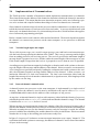
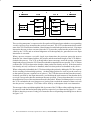
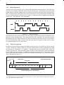
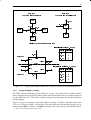
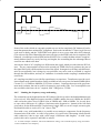
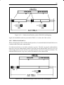
In figure 2.4, a process P is about to execute an output instruction on an ‘empty’ channel C. The
evaluation stack holds a pointer to a message, the address of channel C and a count of the number
of bytes in the message.
19
j
fgZhgc i@`GZDe4i
k
\MUVE]_^DY%`
TU%VWEXPYDYZD[
NotProcess
a UbD]2cdY%`GZDe
Figure 2.4
Output to empty channel
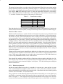
After executing the variable output instruction, the channel C holds the address of the workspace
of P, and the address and length of the message to be transferred are stored in the workspace, as
shown in figure 2.5. P is descheduled, and the processor starts to execute the next process from
the scheduling list.
a
p
qr]2eosiEbXVEZ
p
lZ%m`
cdYi3`neo^V(`nc ]2Y
t<ZDYh`nW
p]2c!Y<`GZDe
Figure 2.5
Outputting Process Descheduled
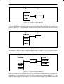
The channel C and the process P remain in this state until a second process, Q executes a variable
input instruction on the channel, as shown in figure 2.6.
a
p
u
\UVE]2^DY<`
qr]_eosiEbXVEZ
p
l Z%m`
cdYi3`neo^V(`nc ]2Y
TU<VWXPYYZD[
a Ub]2c!Y<`GZDe
t<ZDYh`nW
pD]2c!Y<`GZDe
Figure 2.6
Input on a Ready Channel
Since the channel is not empty, the message is copied and the waiting process P is added to the
scheduling list. The channel C is reset to its initial ‘empty’ state, as shown in figure 2.7. The
length of the message (as specified by P) is recorded in the workspace of Q so that it can be put
onto the stack by the load count instruction.
20
‹
‡
ƒr2}„|…†€w
vwx@y
z!{E|@yn}~€ynz 2{
ˆ
NotProcess
‚Ez |@y
‚<wD{‰ynŠ
Figure 2.7
Communication completed, output ready first
If P is the receiving process and Q the sending one, the same set of pictures apply, except that
the final state is as shown in figure 2.8.
‡
ˆ
‹
ƒr2}„|…†€w
vŒw%x@y
z!{E|@yn}~€(ynz 2{
NotProcess
‚z |3y
‚<wD{‰ynŠ
Figure 2.8
2.4.3
Communication completed, input ready first
External channel communication
The synchronised message passing of the transputer requires that data be copied from the sending
process to the receiving process, and that the sending process continue execution only after the
receiving process has input the data. Where the processes communicating reside on different
transputers, it is necessary to transfer the data from one transputer to the other, and to signal in
the other direction that an input has occurred. Thus the connection between the processes must
convey information in both directions.
Virtual links
In the first–generation transputers, each point-to-point physical link between transputers provides two communication channels, one in each direction. In the new transputers, each physical
link provides an arbitrary number of point-to-point virtual links. Each virtual link provides two
channels, one in each direction. Hardware within the transputer multiplexes virtual links onto
the physical links. At any moment, each physical link has an associated list of virtual links waiting to use it.
Each virtual link is represented by a pair of virtual link control blocks (VLCBs), one on each
transputer. When a process executes an input or output instruction to send or receive a message
on a virtual link, the process is descheduled and its identity is stored in the control block. At the
same time the control block is used to determine the physical link to be used for the communication, and is added to the associated list of waiting virtual links. An example of how the lists might
look at one moment is illustrated in figure 2.9.
21
VLCBs
VCP Registers
Link 0
Link 1
Front
Back
Front
Back
Figure 2.9
Queues of VLCBs
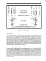
Message–passing Protocol
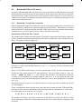
When an output is performed, the message is transmitted as a sequence of packets, each of which
is restricted in length to a maximum of 32 data bytes. There are several reasons for this which
are explained below. Each packet of the message starts with a header, which is used to route the
packet to an receiving process on a remote transputer. The header also identifies the control block
of the virtual link used by the remote receiving process. Thus a virtual link is established by setting up a control block in each of two transputers such that the header in each control block is
set to cause packets to address the other control block.
Each packet of a message is transferred directly from the sending process to the physical link and
is transferred directly from the physical link to the receiving process, provided that a process is
waiting when the packet arrives. An acknowledgement packet is dispatched back along the virtual link as soon as each packet starts to arrive (thus transmission of acknowledge packets can overlap transmission of message packets). At the outputting end of the virtual link, the process will
be rescheduled after the last acknowledgement packet has been received.
When the first packet of a message starts to arrive on a virtual link, it is possible that no process
is waiting to input the message. In this case, it is essential that the packet is stored temporarily
so that communication via other virtual links sharing the same physical link is not delayed. A
single packet buffer associated with each virtual link control block is sufficient for this purpose,
since the outputter will not send any further packets until an acknowledgement packet is received.
The splitting of messages into packets of limited size, each of which is acknowledged before the
next is sent, has several important consequences:
It prevents any single virtual link from hogging a physical link

It prevents a single virtual link from hogging a path through a network



It provides flow-control of message communication and provides the end-to-end synchronization needed for synchronised process communication
It requires only a small buffer to be used to avoid blocking in the case that a message arrives
before a process is ready to receive it
22
Each VLCB must be initialized with the address of the packet buffer for the input channel, the
header to be used for outgoing packets, and which physical link is to be used by the virtual link.
The implementation of message–passing
When a message is passed via a virtual channel the processor of the T9000 delegates the job of
transferring the message to the VCP and deschedules the process. Once a message has been transferred the VCP causes the waiting process to be rescheduled. This allows the processor to continue the execution of other processes whilst the external message transfer takes place.
In figure 2.10 processes P and Q, executed by different transputers, communicate using a virtual
channel C implemented by a link connecting two transputers. P outputs, and Q inputs; note that
the protocol used by the VCP ensures that it does not matter which of P and Q becomes ready
first.
¡
žg”Ÿgœ @™G”D4 ¤¥ š Ž
š
¤¥ š Ž
£
ž¢”Ÿ>œ 3™G”D$ –M—2˜D“<™
–E—2˜D“<™
Ž%‘’P““”D•
Ž%‘’P““”D•
š ›D—_œ!“<™G”P
š ›—2œ!“<™G”D
Figure 2.10
Communication between transputers
The VCP, on being told to output a message, stores the pointer, count and process id into the
VLCB, and causes the first packet of the message to be sent. The VCP maintains queues of
VLCBs for packets to be sent on each link, so the sending of a packet is in two parts; firstly adding
the VLCB to the corresponding queue, and then subsequently taking the VLCB from the front
of the queue and sending a packet, with the header provided by the VLCB. The queues of VLCBs
are illustrated in figure 2.9.
Subsequently, on receipt of an acknowledge packet for this virtual channel, the VCP sends the
next packet of the message. This continues until all packets have been sent. When the final acknowledge is received, the VCP reads the process id from the VLCB and causes the waiting process to be scheduled.
23
­
¦
¯r§2¬o°@±²³´E«
¸¹ ­»º
µ
¸¹ ­¼º
¹E¨ ±@ª
¹E¨ ±@ª
µ
¦
¶«%·ª
¨d©±3ªn¬o®´(ªn¨ §2©
¯r§2¬o°±E²³´E«
¦D§2¨d©%ªG«D¬
¦§2¨!©<ªG«D¬
­ §2®D©%ª
­ §2®©%ª
Figure 2.11
¶«·@ª
¨!©E±@ªn¬®´ªn¨ §2©
Communication in Progress
The receiving transputer’s response to the first packet will depend upon whether a corresponding
variable input message instruction has yet been executed. The VCP can determine this from the
state of the VLCB associated with the virtual channel on which the packet has arrived. If an input
instruction has not yet been executed, then the VCP stores the packet into the packet buffer provided by the VLCB, and an acknowledgement will subsequently be generated once an input
instruction is executed.
When a process executes a variable length input instruction, the processor passes the process
identifier, the virtual channel address, the pointer, and the maximum length, to the VCP and deschedules the process. The VCP, on being told to input a message, stores the pointer, maximum
length and process id into the VLCB and records that an input has been requested. The VCP then
examines the VLCB to determine whether a data packet has already arrived. If the data packet
has already arrived, it will now be handled; otherwise data packets are handled as they arrive.
When a data packet is handled, the VCP acknowledges the packet by adding the VLCB to a queue
for the sending of acknowledge packets. (Acknowledge packets are sent in just the same way
as data packets, but use a separate set of queues.) The VCP then stores the data into the memory
locations specified by the input instruction, provided that the total amount of data that has been
received is not greater than the maximum amount specified. If more data than this is received
then all data in excess of the maximum allowed is discarded. When a final data packet is received,
the VCP reschedules the receiving process, having first recorded the amount of data received4
into the process’ workspace. This value will be used by a subsequent load count instruction.
The message is thus copied through the link, by means of the VLCBs at either end being alternately queued to send data and acknowledge packets respectively, as illustrated in figure 2.11. After
all this is done the processes P and Q are returned to the corresponding scheduling lists as shown
in figure 2.12.
4.
If too much data is received, a special error value (= FFFFFFFF½¿¾ ) is recorded instead.
24
É
ÀrÁ2ÂÃÄÅÆÇÈ
ÓÒ%Ê»Ô
ÓÒ%ʼÔ
Ë
ÀrÁ2ÂÃÄÅÆÇEÈ
̌È%Í@Î
Ï!ÐEÄ@ÎnÂÑÇ(ÎoÏ Á2Ð
ÌÈ%ÍÎ
ÏdÐÄ3ÎnÂoÑÇ(ÎnÏ Á2Ð
ÒEÏ Ä3Î
ÒEÏ Ä@Î
Figure 2.12
2.4.4
Ê
Communication completed
Known length communication
In many cases both the sender and receiver of a message know the precise length of the message
to be transferred in advance. In this case it is possible to optimize the operation of message passing and the T9000 provides a number of instructions which do this. The most important of these
are input message and output message 5.
These instructions are like vin and vout except that both the receiver and the sender specify the
actual length of message to be passed. There is no need for an instruction which corresponds to
load count in this case.
The operation of known length internal communication is similar to variable length communication. However, the first process to synchronize does not need to store the length, since the same
length will be specified by the second process.
The operation of known length external communication is identical to the variable length case,
except for the omission of the load count instruction.
2.5
Alternative input
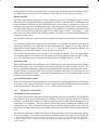
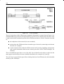
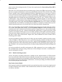
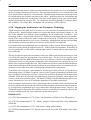
In a system, it is sometimes necessary for a process to be able to input from any one of several
other concurrent processes. For example, consider a process which is implementing a bounded
buffer between two other processes, one of which (a peripheral of some kind) outputs data to the
buffer along a channel, the other (the ”consumer”) requests data from the buffer along another
channel, and receives it via a third, as illustrated in figure 2.13. The behavior of the buffer process
is determined not only by its internal state, but also by whether the other processes wish to add
or to take data from the buffer.
The alternative construct is a means to select between one of a number of guarded processes, each
comprising a guard and an associated process; the guard is typically an input6. The alternative
selects a guarded process whose guard is ready. If a particular guarded process is selected then
both the guard and the associated process are executed. Guards may also have a boolean part
which force the guard to be disregarded if the boolean is FALSE.
5. Note that this is the only form of communication supported by the first–generation transputers.
6. In principle, outputs could equally well be used as guards; however the implementation becomes considerably
more complex if both inputs and outputs are allowed as guards. Thus in the T9000 output guards are not allowed.
25
Peripheral
Consumer
Buffer
Figure 2.13
Buffer process
The T9000’s implementation of alternative separates the selection of a guarded process from its
execution. This means that the only new mechanism needed is one to support selection.
The idea behind the selection mechanism is that for each guard, the channel is examined to see
if it is ready. If, when all the channels have been examined, no ready channel has been found,
the process deschedules until at least one is ready. The process then re–examines the channels
and chooses the first one that it finds ready. The key to the mechanism is therefore, the means
by which a process can deschedule until one of several channels becomes ready.
The first aspect of this mechanism is that channels can be enabled and disabled. A channel is
enabled (by the process performing the alternative) by executing an enable channel instruction.
One effect of this instruction is that if the channel subsequently has an output performed on it,
the output will signal the process performing alternative that the channel has become ready. An
enabled channel is disabled by the process performing alternative executing a disable channel
instruction, which reverses the effect of an enable channel instruction.
The second aspect of the mechanism is the use of a special workspace location by the process
performing alternative. This location serves a number of purposes. Firstly, in the case of a
straightforward input it is used to hold the pointer to the location to store the message, as discussed
previously; consequently it is referred to as the ”pointer location”. Secondly, whilst an alternative is being performed, it contains one of the special values Enabling (= NotProcess + 1),
Waiting (= NotProcess + 2), or Ready (= NotProcess + 3). As no process which is
performing a normal input could be descheduled with one of these values in its pointer location
(processes being forbidden to input messages to these addresses), the value in the location distinguishes a process performing alternative from an inputting process. Thirdly, it is used to record
whether any channel which has been examined is ready. Finally, it is also used to record whether
a process performing alternative is active or descheduled.
The implementation of alternative can now be explained.
Alternative start
The first thing that a process does to perform an alternative is to execute an alternative start
instruction. This sets the pointer location of the workspace to the value Enabling, indicating
that an alternative is in progress, that no guard has yet been seen to be ready, and that the process
performing alternative is active.
Enable channel
The process performing alternative then executes an enable channel instruction for every channel
guard. This instruction determines whether the channel is ready, and, if it is not ready, the instruc-
26
tion enables it. If, on the other hand, the channel is ready the instruction sets the value in the
pointer location to Ready.
For an internal channel, the processor determines whether a channel is ready by examining the
channel word. If it contains the identity of another process, then that process has performed an
output on the channel, and so the channel is ready. Otherwise, the channel is empty, and so is
enabled by writing inti it the process id of the process performing alternative.
For a virtual channel, the processor uses the VCP to enable the channel. The VCP examines the
VLCB of the channel; if the packet buffer already contains the first packet of a message then the
channel is ready. Otherwise, the VCP records in the VLCB that the channel has been enabled.
Alternative wait
Once a process has enabled all the channels from which it wishes to make a selection, it executes
an alternative wait instruction. This first writes the value -1 to location 0 of the workspace, in
preparation for the selection process. Then, if the pointer location still contains the value Enabling, indicating that no guard is yet ready, the instruction writes the value Waiting into the
pointer location, indicating that the process performing alternative is not active, and deschedules
the process. Otherwise, the pointer location contains Ready, indicating that at least one guard
is ready, so the process continues to make its selection.
If a process deschedules on execution of an alternative wait instruction, it will be scheduled when
one of the guards becomes ready. The process will then proceed to make its selection.
Output on an enabled channel
When an output occurs on an internal channel which contains a process id, the sending process
distinguishes between a channel which is ready for input and a channel which is ready for alternative input by examining the pointer location of the waiting process. If this word contains one of
the special values Enabling, Waiting, or Ready then the channel is in use by a process performing an alternative. In this case the sending process will store information into its own workspace and deschedule as if the inputter were not ready, and may also perform some other actions,
depending on the value in the pointer word of the receiving process:
Õ
Õ
If the value is Enabling then the output instruction changes the value to Ready, indicating that an enabled channel is ready.
Õ
If the value is Waiting, and hence the process performing alternative is descheduled,
then the output instruction changes the value to Ready, and schedules the process performing alternative.
If the value is Ready, the output instruction performs no additional action.
When an output occurs on an enabled virtual channel, the VCP of the outputting transputer will
send the first packet of the message as usual; indeed, the sending transputer has no indication that
the channel has been enabled. When the first packet arrives on an enabled virtual channel, the
VCP places the packet in the packet buffer, and records that a packet has arrived as is normal for
for a channel on which no input has been performed. The VCP also informs the scheduler that
an enabled channel has become ready. The scheduler will then examine the pointer word of the
process which enabled the channel and performs the same actions as an output instruction
executed by a local process, as described above.
Once an output has been performed on an enabled channel two conditions are true; firstly, that
the process performing alternative is active (either because it has not descheduled, or because a
channel which has become ready has scheduled it); and secondly, the pointer word of the process
performing alternative has the value Ready. These two, together with the condition for desche-
27
duling when an alternative wait instruction is executed, ensure that a process executes the instruction following an alternative wait instruction if, and only if, at least one guard is ready.
Disable channel
The process performing alternative selects a guarded process by executing a disable channel
instruction for each guard and then executing an alternative end instruction. In addition to the
channel address, the disable channel instruction takes a code offset as a parameter. This is the
offset from the alternative end instruction to the code for the guard. If the disable channel instruction finds that a channel is ready, then workspace 0 is examined; if it contains a value other than
-1 then a selection has already been made, so no further action is taken. If it contains -1 then
this is the first ready channel to be disabled and the code offset associated with this channel is
written into workspace 0.
The operation of disable channel depends on whether the channel is internal or is a virtual channel.
For an internal channel, the channel word is examined. If it contains the identity of the process
performing alternative, an output has not been performed, the channel is not ready, and the
instruction resets the channel word to NotProcess . If the channel contains the identity of a
sending process, then the channel is ready and may be selected.
For a virtual channel, the processor uses the VCP to disable the channel. The VCP examines the
VLCB of the channel; if it contains the first packet of a message then the channel is ready. Otherwise, the VCP removes the information that the channel is enabled from the VLCB.
Alternative end
When all the guards have been disabled, one will have been selected, because guards are not disabled until at least one is ready, and the first ready guard that is disabled will be selected. The
process performing alternative jumps to the code corresponding to the selected guard by executing the alternative end instruction. This instruction reads the code offset from workspace 0, and
adds it to the instruction pointer. In this way the guarded process corresponding to the selected
channel is caused to be executed.
A note about boolean guards
In the above, the fact that the guarded processes can have boolean guards has been overlooked.
In fact, the enable channel and disable channel instructions take an additional parameter which
is the boolean guard. If the guard is FALSE (= 0) they perform no action.
2.5.1
Extensions of alternative
Prioritized and fair alternatives
The T9000’s alternative mechanism actually implements a prioritized alternative, the guards being prioritized in the order in which they are disabled. This can be directly useful; for example,
consider a bounded buffer where we wish to prioritize receiving data from the peripheral over
supplying it to a consumer. This can easily be achieved by always disabling the channel to the
consumer process7 first, so that if both the peripheral and the consumer happen to be ready, the
alternative end instruction will always find the offset to the code which interacts with the peripheral.
The prioritized alternative which is actually provided can also be used to implement fair alternatives. For example, if we wish to ensure that the bounded buffer on average favours neither the
7. Since the implementation only provides for input guards, it is necessary to use two channels between the buffer
and the consumer process, so that the consumer can perform an output to the buffer to indicate its readiness to
receive an item.
28
peripheral nor the consumer, then this can be achieved by always disabling first the channel which
was not selected on the previous iteration of the buffer control loop.
Other guards
In addition to inputs from channels, alternatives allows two other types of guard which may be
used in addition to, or instead of channel guards.
The first is a SKIP guard, which is always ready. This guard is useful in conjunction with boolean
guards, and is supported by the enable skip and disable skip instructions.
The second is a timer guard, which can be used for implementing timeouts, or for arranging for
several different time related operations to be scheduled by a single process. The implementation
of timer guards is built upon the implementation described above. However, some extra mechanisms are needed, and this necessitates the use of the timer alternative start and timer alternative
wait instructions, rather than alternative start and alternative wait, for any alternative which contains timer guards. Timer guards are supported by the enable timer and disable timer instructions.
2.6
Shared channels and Resources
2.6.1
Alternative
The alternative mechanism is very general. It allows a choice to be made between channels,
SKIPs and timers; each guard of an alternative may contain a boolean part; and the choice between guards is prioritized. Furthermore, there is complete freedom about how the channels are
used both within and outside the alternative. It is this generality that necessitates the enabling
and disabling of all the guards every time an alternative is executed, a consequence of which is
that the cost of an alternative is proportional to the number of guards. This cost is incurred every
time a selection is made.
Users
Channels:
Server
Figure 2.14
2.6.2
Server and users
Servers
One common use of an alternative is to implement a server, or to provide access to a resource.
For example figure 2.14 illustrates the notion of a simple server which offers a service to N users,
each connected to the server by one of an array of channels.
As the provision of the service may involve further interaction with the user, it is necessary for
the code which provides the service to be passed its identity. In this case, the index of the channel
in the array identifies the user.
29
In addition to the potentially large cost of the alternative, there is another potential drawback to
this implementation of a server; this is, that the server must know the identity of all the channels
connecting to users, since it has to enable and disable them in order to select one. A user cannot
use a resource that does not know about the channel along which it communicates. A further difficulty is that fairness between the users is complicated to implement.
The T9000 provides a communication mechanism called a ‘‘resource’’ which overcomes both
of these these problems . A resource may be thought of as a shared channel which connects a
number of ‘‘user’’ processes to a ‘‘server’’ process.
2.6.3
Sharing a channel by a semaphore
Before describing the T9000’s resource mechanism and its use, we will first consider another
mechanism that might be used.
Using an efficient semaphore mechanism (which the T9000 does provide), we could implement
resources by means of a single communication channel, whose use was shared by means of a
semaphore. The resulting system would comprise a channel, used to synchronize with the server,
and a queue of processes waiting to use the server, belonging to the semaphore. Whilst this mechanism would work, it has two drawbacks:
Ö
It is not a distributed mechanism – it would work only on a single transputer.
Ö
It no longer allows channels to be used as an abstraction. Rather than merely communicating via a channel, a user would have to first claim the semaphore.
The resource mechanism overcomes both of these problems.
2.6.4
Resources
A resource connects a number of user processes to a single server process. The resource comprises a number of resource channels, one for each user, and a resource data structure (RDS).
A user process communicates with the server by outputting on its resource channel, exactly as
if it were an ordinary channel. The server selects a resource channel by executing a a grant
instruction with the address of the RDS. Once a user process has output on a resource channel,
the grant will deliver the identifier of the chosen resource channel to the server. The server can
then input from the chosen resource channel. Thus the operation of a resource is like that of an
alternative, in that the functions of selection and communication are separated.
The identifier associated with a resource channel is a single word value which is delivered to the
server on completion of a grant. This is the only information delivered to the server to identify
the chosen resource channel, and hence, the user. Although it might seem as though the server
should receive the address of the chosen resource channel, this is not always adequate. For example, in the server shown in figure 2.14 above, the service–providing code may need the index of
the channel rather than the channel itself, so that it can use this index in an array of reply channels.
On the other hand, if the channel address is what is wanted, then the identifier can be set to be
the channel address.
Resource data structure
The resource data structure contains one word used to synchronize the server process with a user
process, and a pair of words used to implement a queue. Unlike a channel shared by a semaphore,
the queue is not a queue of waiting processes, but a queue of resource channels, each of which
has been output to by a user process.
30
Back of Queue
Front of Queue
Synch word
Figure 2.15
Resource Data Structure (RDS)
An RDS is initialized by setting both the synchronization word and the front pointer to NotProcess .
Resource channels
A resource channel is a channel together with an a pair of words. In the case of a virtual resource
channel, the extra pair of words are associated with the VLCB of the receiving (resource) side.
The address of a resource channel does not distinguish it from an ordinary channel, and a resource
channel which is not currently part of a resource may be used used just like an ordinary channel,
in which case the pair of words is not used.
Resource instructions
In addition to the output instructions mentioned previously, there are three instructions provided
to implement the resource mechanism. These are:
×
mark resource channel
×
grant
×
unmark resource channel
The operation of mark resource channel
The resource mechanism allows resource channels to be made part of a resource (‘‘marked’’) by
either the server or by the user8. A server may mark a resource channel irrespective of when the
user outputs on the channel; a user must mark a resource channel prior to outputting on the channel.
A resource channel is marked as being part of a resource by the execution of a mark resource
channel instruction. This instruction takes three parameters; a pointer to the resource channel,
the identifier, and a pointer to the RDS. There are two possibilities: either the channel is empty,
or an output has already occurred.
If the channel is empty, then the identifier and the pointer to the RDS are stored in the extra words
associated with the channel. For an internal channel, the special value ResChan (= NotProcess + 2) is written into the channel word to indicate that it is part of a resource; for an external
channel the VCP records this in the VLCB. This is illustrated in figure 2.16.
8. A user located on a different transputer from the server must arrange for a process local to the server to
do this. This is discussed in section 2.7.3.
31
Channel Identifier
RDS
Process workspace
Pointer to RDS
Channel:
In resource mode
Figure 2.16
Channel after mark resource channel but before output
If an output has already been executed on the channel, then the mark resource channel instruction
must be being executed by the server. In this case the channel will be queued on the RDS, using
the first of the pair of words to form a linked list, with the second extra word containing the identifier. This is illustrated in figure 2.19.
The operation of grant
A server process grants use of a resource by loading the evaluation stack with a pointer to the
resource data structure and a pointer to a location which is to receive the identifier of the granted
resource channel, and then executing a grant instruction.
If there is a resource channel on the queue, it is dequeued and its identifier is written into the location provided for it. The server then continues and can input from the (now unmarked) resource
channel.
RDS
Process workspace
Empty
Channel:
Pointer to server
Server
Id location
Pointer to location
Figure 2.17
RDS and Server after grant
If there is no resource channel on the queue, then there is no user process waiting for the resource.
In this case the instruction writes the process id of the server into the synchronization word of
32
the RDS, writes the address to where the identifier will be written into the workspace of the server
and deschedules it. This is illustrated in figure 2.17. The server will be rescheduled when a user
outputs to the resource. Thus the resource mechanism also provides non–busy waiting, just like
alternative.
Note that once a resource channel is granted to a resource it becomes unmarked. It must be re–
marked before it can be used as part of the resource again. In the meantime it can be used as a
normal channel.
The operation of output
An output performed on a unmarked resource channel is indistinguishable from an output on an
ordinary channel, as illustrated in figure 2.18.
Process workspace
Channel:
Pointer to process
Figure 2.18
Channel after output only
When an output is performed on a marked internal channel, the output instruction reads the channel word in the normal way. On discovering that it contains the special value ResChan, indicating that it is a marked resource channel, the instruction reads the pointer to the RDS from one
of the extra words of the resource channel and examines the RDS.
If there is no server present in the RDS, the output instruction queues the resource channel onto
the RDS, as shown in figure 2.19. If there is a server present, then the instruction grants the channel to the server; the channel word is set to the process id of the sending process, the resource
channel’s identifier is written into the address specified in the pointer location of the server’s
workspace, and the server is rescheduled, as shown in figure 2.20.
33
Channel Identifier
RDS
Client Processes
Channel Identifier
Channel Identifier
Channel Identifier
Figure 2.19
Four resource channels after mark resource channel and output
When an output is performed on a marked virtual resource channel the first packet is transmitted
in the normal way. Indeed, there is no indication at the output end of the virtual channel that the
channel is a resource channel. When the packet arrives at the receiving transputer, the VCP will
notice that the packet has arrived on a marked resource channel, and cause the associated RDS
to be examined by the scheduler. If there is no process id of a server present in the RDS, then
the scheduler queues the resource channel on the RDS as shown in figure 2.19. If there is a process id in the RDS, then the channel is unmarked and granted to the server. The scheduler reads
the pointer to where the server wishes the identifier to be stored from the server’s pointer location,
stores the identifier there, and reschedules the server as shown in figure 2.20.
34
Client Processes
RDS
Channel Identifier
Server
Channel Identifier
Channel Identifier
Channel Identifier
Figure 2.20
RDS with queued resource channels and server after grant
Note that in both the internal and external case the resource channel is then in the same state as
a channel after an output has been performed and before the corresponding input has been performed, as shown in figure 2.18.
2.7
Use of resources
The T9000’s resource channel mechanism can be used in several ways, three of which we now
discuss.
2.7.1
Resources as a replacement for alternative; Omniscient servers
Consider the server example shown in figure 2.14, in which a set of users request some service
from a server by communicating on an array of channels. We assume that the central server process repeatedly chooses a user which has requested it, provides some service for a time, and then
chooses another user. If no user requires the service, the server will wait non–busily.
Although this can be implemented directly using the T9000’s alternative mechanism, the cost
may be too high if there are a large number of users, and the time taken to perform the service
is small. However, if this is so, we can implement the above server using a resource.
The server process first creates and initializes a resource data structure, and then marks all of the
resource channels in the array as being part of that resource. The identifier of each resource chan-
35
nel is set to the index of that channel in the array. The server then repeatedly selects a user by
performing grant, inputs from the chosen user and provides the service. The granting of the chosen channel enables it to be used as an ordinary channel, and so the server has to re-mark the channel to include it in the resource when the server has completed this iteration. Finally, if and when
the server terminates, the channels may have to be placed in a state where they can be used again
as ordinary channels. This is done by means of the unmark resource channel instruction.
In order that the new code works correctly, the channels must have been allocated as resource
channels. This can be achieved either by allocating all channels as resource channels, or by allocating only those channels used in resources as resource channels, in order to optimize memory
usage.
This implementation has a one-off set up and take down cost, proportional to the number of users,
and a constant per-iteration cost which is independent of the number of users. The users (sending
processes) cannot distinguish between this implementation and one using alternative – or indeed
one in which every user is provided with its own server, which simply performs input!
The use of resources instead of alternative is efficient only where a number of constraints are obeyed. Boolean guards and explicitly prioritized selection must be avoided, and the server process
must interact with only the selected user, and not with any other users.
2.7.2
Resources in alternatives
Although the above has been suggestive that resources are some sort of a replacement for alternatives, they are in fact complementary. Resources may be used as guards in alternatives by means
of the enable grant and disable grant instructions.
The use of resources in this way is very natural. For example, consider a bounded buffer process,
with several providers of data and several users thereof, as illustrated in figure 2.21.
Users
Server
Providers
Figure 2.21
Server with users and inputs
This can be implemented using two resources, one for the users and one for the providers. The
server can use an alternative to select between the users as a group and the providers as a group,
and then within each branch of the alternative it can make a further selection by the resource
mechanism as already described. This ensures that the server will wait (non–busily) until either
36
a user or a provider is ready to communicate. When there are many inputs and users waiting,
the server can prioritize either users or providers within the alternative as previously explained.
2.7.3
Ignorant servers
We have seen how to use resources instead of alternatives. In that case, the server knows through
which channels its users communicate, and how many users there are, but the users are unable
to distinguish the resource from an alternative. We now consider how resources can be used when
the server and the users know only the location of the RDS. In this case the resource channels
can be generated dynamically as needed.
We start by explaining how to do this where the users are located on the same transputer as the
server, and then we explain how to do this where the users and server may be located on different
transputers.
Local server and users
In this case the user knows that it is going to use a resource channel and knows the RDS of the
resource. The user allocates three words of memory for use as a resource channel, initializes the
channel part to NotProcess, and executes a mark resource channel instruction which specifies
the RDS of the resource and gives the address of the channel itself as the identifier of the channel.
The user then performs an output on the channel. The server, when it grants this resource channel,
will be delivered the address of the channel, and can then input from the user. In practice, it will
probably be necessary for the resource to be able to output to the user, as well as the user outputting to the resource. A channel can be established in the reverse direction according to some convention known both to user and server.
Distributed servers and user
The distributed case is more complex because the user cannot initialize and mark a resource channel by itself. Firstly, as the user and server are located on different transputers, a virtual resource
channel must be used. It must first be allocated, then both ends of the virtual link must be initialized. Once this has been done something must mark the input side of the virtual channel; this
something must be executed on the same transputer as the server, not on the same transputer as
the user!
However, if we assume the existence of a distributed kernel, capable of allocating, initializing
and marking virtual channels, the distributed case becomes straightforward. Firstly, the user asks
the kernel to initialize and mark a virtual channel connected to the server9. The kernel then cooperates with the kernel on the server’s machine to initialize the virtual channel, and then the local
kernel waits for the remote kernel to mark the virtual channel. The local kernel then informs the
user process of which virtual channel to use, and the user process proceeds to output on that channel.
2.8
Conclusion
The T9000 transputer and C104 router provide the mechanisms necessary for the construction
of large concurrent distributed systems. The T9000 provides a process and communication model, based around synchronised message passing over unidirectional point-to-point channels including an efficient and non-busy implementation of message passing, alternative and resources.
The communication system of the T9000 enables channels to be established between processes
executing on different transputers, and for the same communication model to be maintained
whether processes are located on a single transputer, or on a number of transputers.
9.
The kernel can appear as a local server to the user.
37
When two T9000 transputers are directly connected, many virtual channels are provided in each
direction between processes on the two transputers. If C104 routers are used, a network may be
built which allows processes distributed over any number of transputers to communicate. The
scheduling and communication mechanisms of the T9000 provide efficient support for a wide
variety of operating system kernel functions and concurrent programming constructs.
38
39
3
3.1
DS-Links and C104 Routers
Introduction
Millions of serial communication links have been shipped as an integral part of the transputer
family of microprocessor devices. This ‘OS-Link’, as it is known, provides a physical point–to–
point connection between two processes running in separate processors. It is full–duplex, and
has an exceptionally low implementation cost and an excellent record for reliability. Indeed, the
OS-Link has been used in almost all sectors of the computer, telecommunications and electronics
markets. Many of these links have been used without transputers, or with a transputer simply
serving as an intelligent DMA controller. However, they are now a mature technology, and by
today’s standards their speed of 20 Mbits/s is relatively low.
Since the introduction of the OS-Link, a new type of serial interconnect has evolved, known as
the DS-Link. A major feature of the DS-Link is that it provides a physical connection over which
any number of software (or ‘virtual’) channels may be multiplexed; these can either be between
two directly connected devices, or can be between any number of different devices, if the links
are connected via (packet) routing switches. Other features include detection and location of the
most likely errors, and a transmission speed of 100 Mbits/s, with 200 Mbits/s planned and further
enhancement possible.
Although DS-Links have been designed for processor to processor communication, they are
equally appropriate for processor to memory communication and specialized applications such
as disk drives, disk arrays, or communication systems.
3.2
Using links between devices
DS-Links provide point–to–point communication between devices. Each connected pair of DSLinks implements a full–duplex, asynchronous, flow–controlled connection operating at a programmable speed of up to 100 MBits/s or more. Point to point links have many advantages over
bus based communications in a system with many devices:
There is no contention for the communication mechanism, regardless of the number of
devices in the system.
There is no capacitive load penalty as more devices are added to the system.
The communications bandwidth does not saturate as more communicating devices are
added to the system. Rather, the larger the number of devices, the greater the total communications bandwidth of the system.
Removing the bus as a single point of failure improves the fault–tolerance of the system.
For small systems, a number of DS-Links on each device can provide complete connection between a few devices. By using additional message routing devices, networks of any size and
topology can be built with complete connection between all devices.
3.3
Levels of link protocol
As with most communications systems, the links can be described at a number of levels with a
hierarchy of protocols. The lowest level of electrical signals is considered in detail in chapter
4.
40
3.3.1
Bit level protocol
To achieve the speed required, a new, simple link standard has been produced. DS-Links have
four wires for each link, a data and ‘strobe’ line for each direction. The data line carries the actual
signal, and the strobe line changes state each time the next bit has the same value as the previous
one10. By this means each DS pair carries an encoded clock, in a way which allows a full bit–time
of skew–tolerance between the two wires. Figure 3.1 shows the form of signals on the data and
strobe wires. All signals are TTL compatible.
Figure 3.1
Link data format
Since the data–strobe system carries a clock, the links are asynchronous; the receiving device synchronizes to the incoming data. This means that DS-Links ‘autobaud’; the only restriction on
the transmission rate is that it does not exceed the maximum speed of the receiver. It also simplifies clock distribution within a system, since the exact phase or frequency of the clock on a pair
of communicating devices is not critical.
3.3.2
Token level protocol
In order to provide efficient support for higher level protocols, it is useful to be able to encode
‘‘tokens” which may contain a data byte or control information (in other standards these might
be referred to as ‘‘characters” or ‘‘symbols” – note that they have no relation to the ‘‘token” of
a token–ring network). Each token has a parity bit plus a control bit which is used to distinguish
between data and control tokens. In addition to the parity and control bits, data tokens contain
8 bits of data and control tokens have two bits to indicate the token type (e.g. ‘end of message’).
This is illustrated in figure 3.2.
Control bit
Data token
Parity bit
P
End of packet token
8 Data bits
0
D
D
D
D
D
D
D
D
P
1
0
1
Scope of parity bit in second token
Figure 3.2
Token level protocol
10. NB: This does not correspond with the usual meaning of ‘strobe’, which would be a signal which indicates
every time that another signal is valid.
41
The parity bit in any token covers the parity of the data/control flag in the same token, and the
data or control bits in the previous token, as shown in figure 3.2. This allows an error in any single
bit of a token, including the token type flag, to be detected even though the tokens are not all the
same length. Odd parity checking is used. To ensure the immediate detection of errors null tokens are sent in the absence of other tokens. The coding of the control tokens is shown in table
3.1, in which P indicates the position of the parity bit in the token.
Table 3.1
!
*+-,.#/102-)
*+-,./7689)9)2:7
*59!201<=!
@BA )
Control token codings
#"$
*34%
*34;
*>?"
@DCBE
%'&)((
%'&)(5&
%'&&)(
%'&&&
*>'"%'&)((
Note that the token level of the protocol is independent of details of the higher levels, such as the
amount of data contained in a packet, or the particular interpretations of packets of different types.
Token level flow control
Token level flow control (i.e. control of the flow of tokens between devices) is performed in each
link module, and the additional tokens used are not visible to the higher–level packet protocol.
The token–level flow control mechanism prevents a sender from overrunning the input buffer
of a receiving link. Each receiving link input contains a buffer for at least 8 tokens (more buffering than this is in fact provided). Whenever the link input has sufficient buffering available for
a further 8 tokens, a flow control token (FCT) is transmitted on the associated link output, and
this FCT gives the sender permission to transmit a further 8 tokens. Once the sender has transmitted a further 8 tokens it waits until it receives another FCT before transmitting any more tokens. The provision of more than 8 tokens of buffering on each link input ensures that in practice
the next FCT is received before the previous batch of 8 tokens has been fully transmitted, so the
token level flow control does not restrict the maximum bandwidth of the link. This is analyzed
in detail in chapter 6.
Token level flow control greatly simplifies the higher levels of the protocol, since it prevents data
from being lost due to buffer overflow and so removes the need for re–transmission unless errors
occur. To the user of the system, the net result is that a connected pair of DS-Links function as
a pair of fully handshaken FIFOs, one in each direction.
Note that the link module regulates the flow of data items without regard to the higher level objects that they may constitute. At any instant the data items buffered by a link module may form
part or all of one or more consecutive higher–level objects. FCTs do not belong to such objects
and are not buffered.
3.3.3
Packet level protocol
In order to transfer data from one device to another, it is sent as one or more packets (in some
other serial standards these might be called ‘‘frames” or ‘‘cells”). This allows a number of simultaneous data transfers to be interleaved on the same link. It also allows data to be routed by packet
switches such as the IMS C104 (described later).
Every packet has a header defining the destination address followed by zero or more data bytes
and, finally, a ‘terminator’ token, which may be either an ‘end of packet’ or an ‘end of message’
token. See figure 3.3. This simple protocol supports data transfers of any length, even when (for
reasons of smooth system performance) the maximum packet size is restricted; the receiving de-
42
vice knows when each packet and message ends without needing to keep track of the number of
bytes received.
header
data bytes
Figure 3.3
3.3.4
terminator
Packet format
Higher level protocols
A variety of higher level protocols can be layered on top of this basic system. DS-Link packets
can be used as a transport mechanism for protocols defined by other standards such as ATM, SCI
and FibreChannel. They also provide very efficient support for synchronised channel communication, as described below.
3.4
Channel communication
A model of communication which can be implemented very efficiently by DS-Links is based on
the ideas of communicating sequential processes. The notion of ‘process’ is very general, and
applies equally to pieces of hardware and pieces of software. Each process can be regarded as
a ‘‘black box” with internal state, which can communicate with other processes using communication channels. Each channel is a point–to–point connection between two processes. One process always inputs from the channel and the other always outputs to it. Communication is synchronized: the first process ready to communicate waits until the second is also ready, then the
data is copied from the outputting process to the inputting process and both processes continue.
Because a channel is external to the processes which use it, it provides a connection between them
which hides their location and internal structure from each other. This means that the interface
of a process can be separated from its internal structure (which may involve sub–processes), allowing the easy application of structured engineering principles.
3.4.1
Virtual channels
Each OS-Link of the original transputers implemented only two channels, one in each direction.
To map a particular piece of software onto a given hardware configuration the programmer had
to map processes to processors within the constraints of available connectivity. The problem is
illustrated in figure 3.4 where 3 channels are required between two processors, but only a single
link connection is available.
One response to this problem is the addition of more links. However this does not really solve
the problem, since the number of extra links that can be added is limited by VLSI technology.
Neither does this ‘solution’ address the more general communication problems in networks, such
as communication between non-adjacent processors, or combining networks in a simple and regular way.
43
Process
A
Process
D
?
Process
B
Process
E
Process
C
Figure 3.4
Multiple communication channels required between devices
A better solution is to add multiplexing hardware to allow any number of processes to use each
link, so that physical links can be shared transparently. These channels which share a link are
known as ‘virtual channels’.
Process
A
Process
D
Mux/
Demux
Process
B
Mux/
Demux
Process
E
Process
C
Figure 3.5
Shared DS-Links between devices
Virtual links
Each message sent across a link is divided into packets. Every packet requires a header to identify
its channel. Packets from messages on different channels are interleaved on the link. There are
two important advantages to this:
F
F
Channels are, generally, not busy all the time, so the multiplexing can make better use
of hardware resource by keeping the links busy with messages from different channels.
Messages from different channels can effectively be sent concurrently – the device does
not have to wait for a long message to complete before sending another.
44
A
G
G
G
G
G
G
G
G
G
B
A
G
G
G
G
G
G
G
G
Mux/
GDemux
B
G
G
G
G
G
G
G
G
G
G
G
G
Packets arriving on link
G
G
G
G
G
G
G
G
B
Figure 3.6
Multiple channels sharing a link
In this specific protocol, a packet can contain up to 32 data bytes. If a message is longer than 32
bytes then it is split up into a number of packets all, except the last, terminated by an ‘end of packet’ token. The last packet of the message, which may contain less than a full 32 bytes, is terminated by an ‘end of message’ token. Shorter messages can be sent in a single packet, containing
0 to 32 bytes of data, terminated by the ‘end of message’ token. Messages are always sent using
the minimum possible number of packets.
Packet acknowledgements are sent as zero length packets terminated with an ‘end of packet’ token. This type of packet can never occur as part of a message because a zero length data packet
must always be the last, and only, packet of a message, and will therefore be terminated by an
‘end of message’ token. Each packet of a message must be acknowledged by receipt of an acknowledge packet before the next can be sent. Process synchronization is ensured by delaying
the acknowledgement of the first packet of a message until a process is ready to input from the
channel, and delaying continuation of the outputting process until all the packets of the message
have been sent and acknowledged.
Virtual channels are always created in pairs to form a ‘virtual link’. This means it is not necessary
to include a return address in packets, since acknowledgements are simply sent back along the
other channel of the virtual link. The strict acknowledgement protocol means that it is not necessary to include sequence numbers in the packets, even when the routing network is non–deterministic!
The specific formats of packets used in this system are illustrated in figure 3.7.
45
header
32 data bytes
First
end of packet packet
header
32 data bytes
end of packet
header
1 to 32 data bytes
Last
end of message packet
Long message (greater than 32 bytes)
header
0 to 32 data bytes
end of message
Short message (0 to 32 data bytes)
header end of packet
Acknowledge packet
Figure 3.7
3.5
High Level protocol packet formats
Errors on links
The DS-Links are designed to be highly reliable within a single subsystem and can be operated
in one of two environments, determined by a flag at each end of the link, called LocalizeError.
In applications where all connections are on a single board or within a single box, the communications system can reasonably be regarded as being totally reliable. In this environment errors are
considered to be extremely rare, but are treated as being catastrophic should one occur. If an error
occurs it will be detected and reported. Normal practice will then be to reset the subsystem in
which the error has occurred and to restart the application. This minimizes the overheads on each
communication, but if an error does occur there will be an interruption in the operation of the
system.
For other applications, for instance when a disconnect or parity error may be expected during
normal operation, a higher level of fault–tolerance is required. This is supported by localizing
errors to the link on which they occur, by setting the LocalizeError bit of the link to 1. If an error
occurs, packets in transit at the time of the error will be discarded or truncated, and the link will
be reset automatically. This minimizes the interruption of the operation of a system, but imposes
an overhead on all communications in order to deal with the possibility that data may be lost.
46
3.5.1
Errors detected
The DS-Link token protocol allows two common types of error to be detected. Firstly the parity
system will detect all single bit errors at the DS-Link token level, and secondly, because each output link, once started, continues to transmit an uninterrupted stream of tokens, the physical disconnection of a link can be detected.
Disconnection errors
If the links are disconnected for any reason whilst they are running then flow control and token
synchronization may be lost. In order to restart the link it is therefore necessary to reset both ends
to a known flow control and token synchronization point.
Disconnection is detected if, after a token has been received, no tokens are seen on the input link
in any 1.6 microsecond window. Once a disconnection error has been detected the link halts its
output. This will subsequently be detected as a disconnect error at the other end, and will cause
that link to halt its output also. It then resets itself, and waits 12.8 microseconds before allowing
communication to restart. This time is sufficient to ensure that both ends of the link have observed disconnection and cycled through reset back into the waiting state. The connection may
now be restarted.
Parity errors
Following a parity error, both bit–level token synchronization and flow control status are no longer valid, therefore both ends of the link must be reset. This is done autonomously by the DS-Link
using an exchange–of–silence protocol.
When a DS-Link detects a parity error on its input it halts its output. This will subsequently be
detected as a disconnect error at the other end, and will cause that link to halt its output also, causing a disconnect to be detected at the first end. The normal disconnect behavior described above
will then ensure that both ends are reset (irrespective of line delay) before either is allowed to
restart.
3.6
Network communications: the IMS C104
The use of DS-Links for directly connecting devices has already been described. The link protocol not only simplifies the use of links between devices but also provides hardware support for
routing messages across a network.
The system described previously packetizes messages to be sent over a link and adds a header
to each packet to identify the virtual channel. These headers can also be used for routing packets
through a communication system connecting a number of devices together. This extends the idea
of multiple channels on a single hardware link to multiple channels through a communications
system; a communications channel can be established between any two devices even if they are
not directly connected.
Because the link architecture allows all the virtual channels of a device to use a single link, complete, system-wide connectivity can be provided by connecting just one link from each device
to the routing network. This can be exploited in a number of ways. For example, two or more
networks can be used in parallel to increase bandwidth, to provide fault–tolerance, or as a ‘user’
network running in parallel with a physically separate ‘system’ network.
The IMS C104 is a device with 32 DS-Links which can route packets between every pair of links
with low latency. An important benefit of using serial links is that it is easy to implement a full
crossbar in VLSI, even with a large number of links. The use of a crossbar allows packets to be
47
passing through all links at the same time, making the best possible use of the available bandwidth.
If the routing logic can be kept simple it can be provided for all the input links in the router. This
avoids the need to share the hardware, which would cause extra delays when several packets arrive at the same time. It is also desirable to avoid the need for the large number of packet buffers
commonly used in routing systems. The use of small buffers and simple routing hardware allows
a single VLSI chip to provide efficient routing between a large number of links.
A single IMS C104 can be used to provide full connectivity between 32 devices. IMS C104s can
also be connected together to build larger switch networks connecting any number of devices.
3.6.1
Wormhole routing
The IMS C104 includes a full 32 x 32 non-blocking crossbar switch, enabling messages to be
routed from any of its links to any other link. In order to minimize latency, the switch uses ‘wormhole routing’, in which the connection through the crossbar is set up as soon as the header has
been read. The header and the rest of the packet can start being transmitted from the output link
immediately. The path through the switch disappears after the ‘end of packet/message’ token has
passed through. This is illustrated in figure 3.8. This method is simple to implement and provides very low latency as the entire packet does not have to be read in before the connection is
made.
Minimizing routing delays
The ability to start outputting a packet while it is still being input can significantly reduce delay,
especially in lightly loaded networks. The delay can be further minimized by keeping the headers
short and by using fast, simple hardware to determine the link to be used for output. The
IMS C104 uses a simple routing algorithm based on interval labelling (described in section
3.6.3).
Because the route through each IMS C104 disappears as soon as the packet has passed through
and the packets from all the channels that pass through a particular link are interleaved, no single
virtual channel can monopolize a route through a network. Messages will not be blocked waiting
for another message to pass through the system, they will only have to wait for one packet.
C104 inputs header and
selects outgoing link
Crossbar connects input to
output; header flows through
followed by rest of packet
Packet terminator closes
crossbar connection
Figure 3.8
Device
or
C104
C104
Device
or
C104
Device
or
C104
C104
Device
or
C104
Device
or
C104
C104
Device
or
C104
Packet passing through IMS C104
48
The IMS C104s that the packets pass through do not need to have information about the complete
route to the destination, only which link each packet should be sent out of at each point. Each
of the IMS C104s in the network is programmed with information that determines which output
link should be used for each header value. In this way, each IMS C104 can route packets out of
whichever link will send it towards its destination.
3.6.2
Header deletion
An approach that simplifies the construction of networks is to provide two levels of header on
each packet. The first header specifies the destination device (actually, the output link from the
routing network), and is removed as the packet leaves the routing system. This exposes the second header which tells the destination device which process (actually, which virtual channel) this
packet is for. To support this, the IMS C104 can route packets of any length. Any information
after the initial header bytes used by the IMS C104 is just treated as part of the packet, even if
it is going to be interpreted as a header elsewhere in the system. Any output link of the IMS C104
can be set to do header deletion, i.e. to remove the routing header from the front of each packet
after it been used to make the routing decision. The first part of the remaining data is then treated
as a header by the next device that receives the packet.
SUT-V-W5TX7Y-ZT-Wf[]8ZT^ T-_![
g a Xh[Y-V1^!^ a bcia bLWT g a _T
R
R
R
R
HJILKNM<O)P-Q
SUT-V-W5TX7Y-Z)T-W\[]8ZT^ T-_![
]Y[`7Y[^ a bcd]eM<O)P-Q
Figure 3.9
Header deletion
As can be seen from figure 3.10, by using separate headers to identify the destination device and
a channel within that device, the labelling of links in a routing network is separated from the labelling of virtual channels within each device. For instance, if the same 2 byte header were used
to do all the routing in a network, then the virtual channels in all the devices would have to be
uniquely labelled with a value in the range 0 to 64K. However, by using two 1 byte headers, all
the devices can use virtual channel numbers in the range 0 to 255. The first byte of the header
will be used by the routing system to ensure that the packets reach the appropriate device before
the virtual channel number is decoded.
49
Š |‹?} |Œ1k} } z ˆfl ‡ kLxŽxlk‘miz l ‡ 8ŒŽlk ‡ k-|-’k#px
jUklnmdoprqdos1t<u)v-w#x
yz phl{-|1}
†‡ |ˆˆk} x‰
v'~€-
-#‚'~ƒuu
‚-#-„v'~<‚…
Š Œ-‹?} |Œk} } z ˆ-fl ‡ k4x“Ž-x“lrk#”m•z l ‡ lnmdo–uLŒŽlk ‡ k-|-’5kpx
jUklnmdoprqdos1t<u)v-w#x
yz phl{-|1}
†‡ |ˆˆk} x‰
v
u
v'~€-
v'~€-
Figure 3.10
-
v'~<--
Using header deletion to label a network
The advantages
of using header deletion in a network are:
—
—
It separates the headers for virtual channels from those for the routing network.
—
The labelling of the network can be done independently of the application using the network.
—
There is no limit to the number of virtual channels that can be handled by a system.
By keeping the header for routing short, routing latency is minimized.
Any number of headers can be added to the beginning of a packet so that header deletion can also
be used to combine hierarchies of networks as shown in figure 3.11. An extra header is added
to route the message through each network. The header at the front of each packet is deleted as
it leaves each network to enter a sub-network. This is just like the local–national–international
hierarchy of telephone numbers. Since the operation of the IMS C104 is completely independent
of the length of the packets, the fact that header deletion changes the length of a packet as it passes
through the network causes no problem at all.
50
¡-¢ž-Ÿf£¤¥ ¤¡£žf¬›-«#­!ž£
£ ¤¡®ª¢¡°?±•šž)£n³d¤ r­-´
Ÿž#œ ž£ž-Ÿ.¤šL¤¡£¬7¡£·µ
¢¯¡°?±•šž)£n³d¤ ­d¤˜¸d¹)º»#¢
¢¯¡°²±ªšž)£¼³<¤ ­d¤˜¸d¹)º-»¢
¡-¢)ž-Ÿf£¤¥ ¤¡£ž\¬#›-«#­)ž)£
£ ¤¡®•¢¯¡°²±ªšž£n³d¤ r­-´
Ÿ5žœ ž£ž-Ÿ.¤šL¤¡£¬5¡)£¶µ
˜r™ š-›œ!ž›Ÿ5ž 5¡¢ž-Ÿ\£¤¥™ Ÿžš)£¦™ §
˜h¨ª©-™ h£¡-›1œ“«-›ššžœ“¤šLŸ5ž©-™ «-ž
Figure 3.11
3.6.3
Using header deletion to route through sub-networks
Labelling networks
For each IMS C104 there will be a number of destinations which can be reached via each of its
output links. Therefore, there needs to be a method of deciding which output link to use for each
packet that arrives. The addresses that can be reached through any link will depend on the way
the network is labelled. An obvious way of determining which destinations are accessible from
each link, is to have a lookup table associated with all the outputs (see figure 3.12). In practice,
this is difficult to implement. There must be an upper bound on the lookup table size and it may
require a large number of comparisons between the header value and the contents of the table.
This is inefficient in silicon area and also potentially slow.
ɀÊ7˯ÌÎÍÐÏ7Ñ#ÌÎÍ ÒÏ1Ë¥ÓÊ7ÑÔ5Õ7Ñ'Ö?× Ê
Ø ÓÒÙÚÌÎÕ=Í Ë.ÒÛ#̶ܲÛÌÝ×ÞÍÐÏ+ß
ÍÐÏ+ß ¾
à
à
à
à
½¾¿À-Á²¿-½=Â
ÍÐÏ+ß À
Ã5Å ¿½ Å ¿ÆÀDz¿È²¿ Ä Â
ÍÐÏ+ß Ã
à ½¿ à à ¿ à Á²¿
Ä ½
Ä È²¿-½ Ã
ÍÐÏ+ß Ä
Figure 3.12
Ò'Òß#Û+ÜáÌÑ+Ö²× ÊNÓÊ5âÝÛ+ÍÐÓÊ5ã
à
à Á
Ã5Å
à ½
à Ã
ÀÁ
À#Ç
È
à
à
à
à
à
à
à
ÍÞÏ=ß
ÍÞÏ=ß
ÍÞÏ=ß
ÍÞÏ=ß
ÍÞÏ=ß
ÍÞÏ=ß
ÍÞÏ=ß
Ã
À
Ã
Ã
à
½ Ã
=½ ¾
à
à
à
Ä Â
¾
Labelling a network
½=Â
½ Å
À
À
Ä È
Ä ½
à
à
à
ÍÐÏ+ß
ÍÐÏ+ß
ÍÐÏ+ß
ÍÐÏ+ß
ÍÐÏ+ß
ÍÐÏ+ß
ÍÐÏ+ß
¾
À
Ä
Ä
¾
Ã
À
51
ô€õ7ö¯÷ÎñÐò7ø÷¶ñ ùò1öáúrõ7øûü1ø'ý?þ õ
ÿ úùÚ÷Îü+ñ ö.ù#÷#÷þÞñÞò=ó
ð1ñÐò+ó î
ð1ñÐò+ó æ
7é ëåUéè²åÝì5êåÝìäå
ìí
äåæç
ð1ñÐò+ó é
êî²åêé²å-ê5ëÝåê=í
ð1ñÐò+ó ì
æ-è²åéé²åé7ê
ò#÷¦õ+úø'þ-úù÷ÎñÞò
÷ø'ý?þ õNúõ+ñÐúõ
äNïïï æ-è
ïïï é7ë ïïï ê=î ïïï ë=î
ð1ñÐò+ó é
ð1ñÐò+ó î
ð1ñÐò+ó ì
ð1ñÐò+ó æ
Figure 3.13
Interval labelling
However, a labelling scheme can be chosen for the network such that each output link has a range
of node addresses that can be reached through it. As long as the ranges for each link are non-overlapping, a very simple test is possible. The header just has to be tested to see into which range,
or interval, it falls and, hence, which output link to use. For example, in figure 3.13, a header
with address n would be tested against each of the four intervals shown below:
Interval
Output link
6
n < 18
1
18 n < 25
3
25 n < 40
0
40 n < 50
2
The advantages of interval labelling are that:
It is ‘complete’ – any network can be labelled so that all packets reach their destinations.
It provides an absolute address for each device in a network, so keeping the calculation
of headers simple.
It is simple to implement in hardware – it requires little silicon area which means it can
be provided for a large number of links as well as keeping costs and power dissipation
down.
Because it is simple, it is also very fast, keeping routing delays to a minimum.
Figure 3.14 gives an example of interval routing for a network of two IMS C104’s and six IMS
T9000 transputers showing one virtual link per transputer. The example shows six virtual channels, one to each transputer, labeled 0 to 5. The interval contains the labels of all virtual channels
accessible via that link. The interval notation [3,6) is read as meaning that the header value must
be greater than or equal to 3 and less than 6. If the progress of a packet with the header value
4 is followed from IMS T90001 then it is evident that it passes through both IMS C104s before
leaving on the link to IMS T90004.
52
)+*!
B
( !
&@
+'!
>
,.-0/2143(50687 9:
!
#$)%*!
;
! +&!;+ &!<#$ %&!
Figure 3.14
('!
= #"$ %&!
A
#$'"!
*?
>
( !;$ !; "!;#"$ %&!
Interval routing
It is possible to label all the major network topologies such that packets follow an optimal route
through the network, and such that the network is deadlock free. Optimal, deadlock free labelings
are available for grids, hypercubes, trees and various multi–stage networks. A few topologies,
such as rings, cannot be labeled in an optimal deadlock free manner. Although they can be labeled
so that they are deadlock free, this is at the expense of not using one or more of the links, so that
the labeling is not optimal. Optimal deadlock free labelings exist if one or more additional links
are used.
3.6.4
Partitioning
All the parameters determining the routing are programmable on a per link basis. This enables
an IMS C104 to be used as part of two or more different networks. For example, a single IMS
C104 could be used for access to both a data network and a control network (see figure 3.15).
Partitioning provides economy in small systems, where using an IMS C104 solely for a control
network is not desired, whilst maintaining absolute security. By ensuring that no link belonging
to one partition occurs in any interval routing table in another partition, it is guaranteed that no
packet can be routed from one partition to another, whatever the value of its header.
53
LNM)O^PR$S_U D
C=D)EFa`b M&cdY Zfegce0OheiZM0OQPRTSVU
LjM)OQP=R$SVUJ
CD)EFa`b M&cdY Zfegk&R$Z0O_SR$l ZM0OQPRTSVU
\
] EEE
G D)EHD FI
G EH ] I
G DH J I
\
] EEE
G E
HD'I
G K$H [&I
CD)EF
CD)EF
G] HD)E&I
\
] EEE
G(J H'KI
CD)EF
\
] EEE
pY Zs$l M CD)EFa`b M&cdt8M)OQPuMM4ZfJiZM0OQPRTSVU b
n.Z0O2M4S(o0e8lvOhe4tl Mxw^R$Sl Y Z4U bF$H mye4Zc [
G#] HD)E*I
LNM0OQPRTSVUWJ
G EH ] I
G DH J I
G EHD'I
LNM0OQPRTSVU D
Figure 3.15
3.6.5
n.Z0O2M4S(o0e8ldpqM4l M&k)OrX&Y Z4U
F
G D)EHD FI
G#] HD)E&I
m
[
G EH ] I
X&Y Z4U [
X&Y Z4U E
X*Y Z4U'm
CD)EF
X&Y Z4U D
&X Y Z4U J
G J H'KI
X&Y Z4U F
X&Y Z4U K
G D EHD FI
G K$H [&I
n.Z0O2M4S(o0e8lvOhe4tl Mxw^R$S$l Y Z4U b=EHDH Jze4Zc K
n.Z0O2M4S(o0e8l pqM4l M&k)OrX&Y Z4U
K
G K$H [&I
J
G(J H'KI
E
G DH J I
D
G EHD'I
Using partitioning to enable one C104 to be used by two different networks
Grouped adaptive routing
The IMS C104 can implement grouped adaptive routing. Sets of consecutive numbered links
can be configured to be grouped, so that a packet routed to any link in the set would be sent down
any free link of the set11. This achieves improved network performance in terms of both latency
and throughput.
Figure 3.16 gives an example of grouped adaptive routing. Consider a message routed from
C1041, via C1042, to T90001. On entering C1042 the header specifies that the message is to be
output down Link5 to T90001. If Link5 is already in use, the message will automatically be
11. This is also sometimes called a hunt group.
54
routed down Link6, Link7 or Link8, dependent on which link is available first. The links can
be configured in groups by setting a bit for each link, which can be set to ‘Start’ to begin a group
and ‘Continue’ to be included in a group.
{|)}~©
{=|)}~
§
Œ ’ Q   ‚”
•– ‚g—f˜r™›š$œ8Ÿž¡ T¢z£
 ¤  ’4¥ ¦ ¤$
{|)}~
}
Œ$hŽ4Q
|
{; ‚   ‚4‘’
ª– ‘4«4’¦
{; ‚   ‚4‘’
Š
{; ‚   ‚4‘’
ˆ
~
Œ$hŽ4Q
Œ$hŽ4Q
„
{; ‚   ‚4‘’
‡
ª– ‘4«4’¦
{; ‚   ‚4‘’
†
{; ‚   ‚4‘’
…
Œ$hŽ4Q
‹
ª– ‘4«4’¦
|)}
{; ‚   ‚4‘’
||
Œ$hŽ4Q
“
“
“ˆ |
Œ$h“ Ž4Q
Figure 3.16
€& ‚4ƒ }
€& ‚4ƒ |
€& ‚4ƒ'Š
€& ‚4ƒ‰ˆ
€* ‚ƒ |)}
€* ‚4ƒ'‹
€& ‚4ƒ …
{|)}~ €& ‚4ƒ †
€& ‚4ƒ ‡
€& ‚4ƒ'„
€* ‚4ƒ ~
¨ ‹ } }}
§
¨ ‹ }}}
Grouped adaptive routing
Grouped adaptive routing is also very effective in multi–stage networks such as those illustrated
in figures 7.1 to 7.4. Since all the centre–stage switches are equivalent, all the links from each
first–stage switch towards the centre can be grouped together, allowing a high degree of adaption
to dynamic traffic conditions.
3.7
Conclusion
DS-Link technology provides reliable, high–speed serial communications at low cost, in a simple
form which is suitable for a wide range of applications. A simple protocol, implemented in hardware, keeps overheads down whilst allowing more complex functions to be layered on top of it.
It also permits high–performance routing devices to be constructed, from which efficient systems
of any size can be built to provide very high system bandwidth and fault–tolerance.
55
4
4.1
Connecting DS-Links
Introduction
Digital design engineers are accustomed to signals that behave as ones and zeros, although they
have to be careful about dissipation and ground inductance, which become increasingly important as speeds increase. Communications engineers, on the other hand, are accustomed to disappearing signals. They design modems that send 19200 bits per second down telephone wires that
were designed 90 years ago to carry 3.4KHz voice signals. Their signals go thousands of kilometers. They are used to multiplexing lots of slow signals down a single fast channel. They use
repeaters, powered by the signal wires.
Digital designers do not need all these communications techniques yet. But sending 100Mbits/s
or more down a cable much longer than a meter has implications that are more analog than digital,
which must be taken care of just like the dissipation and ground inductance problems, to ensure
that signals still behave as ones and zeros.
Actually, it is easy to overestimate the problems of these signal speeds. Engineers designing with
ECL, even fifteen years ago, had to deal with some of the problems of transmitting such signals
reliably, at least through printed circuit boards (PCBs), backplanes, and short cables. One of the
best books on the subject is the Motorola ‘MECL System Design Handbook’ [1] by William R
Blood, Jr., which explains about transmission lines in PCBs and cables. This shows waveforms
of a 50MHz signal at the end of 50ft (15m) of twisted pair, and of a 350MHz signal at the end
of 10ft (3m) of twisted pair, both with respectable signals.
This chapter first discusses the signal properties of DS-Links. PCB and cable connections are
then described, followed by a section on error rates: errors are much less frequent on transputer
links than is normal in communications. A longer section introduces some of the characteristics
of optical connections including optical fibre, which should be suitable for link connections up
to 500m, using an interface chip to convert between the link and the fibre. A pointer is given
towards possible standards for link connections. Appendix A describes a connector that will assist standardization of transputer link connections. Appendix B shows waveforms of signals
transmitted through cable and fibre. Appendix C gives detailed electrical parameters of DSLinks, and appendix D gives an equivalent circuit for the DS-Link output pads.
4.2
Signal properties of transputer links
Considerable design work has gone into making the DS-Link signals [4] well behaved. The bitlevel protocol and the electrical characteristics both contribute to make the link signals unusually
easy to use, for serial data at 100MBits/s.
The DS-Link information is carried by a pair of wires in each direction. The D signal carries data
bits, and the S signal is a strobe, which changes level every bit time that the D signal does not
change12. This is illustrated in figure 4.1. This bit-level protocol guarantees that there is a transition on either D or S every bit time. Effectively this provides a Gray code between the D and
S signals.
12. Note that this differs from the usual meaning of a ‘strobe’, which is a signal which indicates every time the
data signal is valid.
56
Figure 4.1
DS-Link signals
One result of the DS Gray coding is that the received data is decoded purely from the sequence
of D and S transitions rather than depending on any absolute time. This means that the link receivers ‘autobaud’, receiving data at whatever speed it is sent (so long as the receiver logic is fast
enough).
The Gray coding makes it much easier to design logic that is fast enough, because the timing resolution required is a whole bit time. Alternative codings would require a clock edge in the centre
of a data bit, and hence require timing resolution of half a bit time. The more relaxed timing resolution needed by the DS-Links gives major benefits in terms of the performance that can be
achieved in practical systems.
A further advantage of the coding, with only D or S changing at a time, is that the signal can be
received without a phase-locked loop (PLL) – the clock is just the Exclusive-OR of the D and
S signals. For the C104 routing switch, avoiding the need for 32 PLLs is very valuable, and it
is likely that a 32 way routing switch would not be implementable had the PLLs been required.
Electrical aspects of the design include a controlled output impedance approximately matched
to a 100 transmission line13. Obviously there is a tolerance on the impedance, which also may
not be identical for high and low, but the DS-Link has been designed to minimize the effect of
any such mismatch on the signal.
The link outputs have also been designed to give controlled rise and fall times. The full electrical
characteristics will not be known until the devices are fully characterized, but a reasonable estimate of the transition times is 3ns fastest transition and 6ns slowest transition.
The DS coding gives as much tolerance as possible for skew between the D and S signals, and
the outputs and inputs have been designed to have minimal skew at the TTL threshold of 1.5V.
These characteristics of the DS-Link signals make them ideal for connections on PCBs, and for
DC coupled connections on short lengths of cable, up to 10m. Later sections will describe such
connections, as well as much longer connections up to 500m using optical methods.
4.3
PCB connections
The following discussion assumes the use of multi-layer PCBs with power and ground planes;
use of DS–Links on double-sided boards without ground planes is not recommended.
A 100 transmission line impedance is fairly easy to achieve on the surface of a PCB. PCBs have
been made with long connections of 100 impedance which carry link signals faithfully. The
100 impedance requires a track width between 0.1mm and 0.3mm, depending on the board
13. See appendix C.
57
thickness and where the power planes are located within it. Figure 4.2 (derived from data given
in Blood [1], from SONY [2], and from Coombs [3]) shows the approximate relationship between these parameters for standard FR4 PCB material with a dielectric constant of 4.7.
Track
width
mm (.001”)
100 on surface
(without soldermask)
0.3
(12)
100 inner
layer
0.2
(8)
0.1
(4)
(approximate, calculated
from data in references)
0
0.1
0.2
0.3
0.4
0.5
0.6
0.7
0.8
0.9
Height of track above ground or power plane (mm)
Figure 4.2
FR4
Graph showing approximate PCB transmission line impedance for FR4 laminate
Note that when a PCB track is buried in the fiberglass/epoxy laminate, its impedance is reduced
by about 20% compared with a surface track. This requires the inner layer tracks to be narrower
than surface tracks, to minimize differences in impedance. It is not possible, within the normal
1.6mm board thickness, to have 100 tracks sandwiched between power or ground planes.
If the transmission line impedance could be maintained with high precision, PCB DS-Link connections would be good for several meters, in theory. However in practice it is hard to maintain
a tighter tolerance than +/– 20%. It is therefore advisable to limit the connections on PCBs to
less than 1000mm with standard FR4 PCB material. If the impedance goes outside the range of
80 to 120 , it is advisable to limit the connection to 500mm.
Short discontinuities in the impedance are permissible, such as connectors, vias, and short sections of track of higher or lower impedance; such discontinuities should be kept to less than
50mm. Similarly, if it is necessary to use some PCB tracks of higher impedance than 100 , and
some lower than 100 , it is best if they can be alternated in short sections, rather than having a
400mm length of 125 track and then a 400mm length of 80 track.
The controlled transition times of the DS-Links minimize crosstalk compared with the sub-nanosecond fall times of some of the fast families of ‘TTL’, but care still needs to be taken over crosstalk. Tests, simulations, and theory using typical PCB materials and DS–Link outputs suggest
that backwards crosstalk increases as the length of the parallel tracks increase up to 25cm, and
58
does not increase for longer parallel tracks. Track separation of 0.15mm over this length appears
to give 1 volt of crosstalk, which is above the noise margin. Simulations of track separation of
1.25mm over a length of 20cm give crosstalk figures of less than 100mV.
The references [1], [2], and [3] do not give a great deal of information about PCB crosstalk, and
the results above suggest that further work is required. In the meantime, it must be good practice
to avoid long parallel runs and to space the tracks out as far as possible. Another technique is to
use guard tracks ( tracks connected to 0V ) between link tracks, although the effects of this on
the impedance of the link track may need to be taken into account.
The D and S pair of signals should be approximately the same length, but a difference in length
of 50mm would only introduce a skew of 250ps, which should be totally acceptable.
4.4
Cable connections
This section looks at existing cable interfaces, comparing them with transputer links, and then
discusses the loss and noise that occur in a cable, and what can be done to overcome their effects.
4.4.1
Existing cable interfaces and rough costs
Ethernet connections are now inexpensive, with a component cost well under $50 and an end-user
cost around $150. Transputer links are even less expensive with a low cost T400 having two OSLinks each capable of 20Mbits/s full duplex, a total bandwidth four times that of ethernet.
Token Ring goes a little faster than Ethernet, but to go substantially faster the next standard is
FDDI at 125 MBits/s (of which 100 Mbits/s are useful data). FDDI is expensive, not only in its
protocol, but even in its components, and just the optical transceiver is not expected to fall below
$100 even in volume for some time.
Links on the T9000 transputer run at 100 MBits/s, full duplex. The cost per link is considerably
less than either the chipset or the transceiver for FDDI. The C104 routing switch, with 32 ports
will give a cost per port well under $10 – at least an order of magnitude less than the FDDI component cost.
Ethernet, Token Ring, and FDDI are all local area networks, with many ports in a network and
long distances between ports. Transputer links are point-to-point, and are generally expected to
be comparatively short connections. In this respect they are more like the recent parallel interfaces such as SCSI2, IPI and HPPI. HPPI as an example has a maximum length of 25m, and runs
at 800 Mbits/s in one direction down a cable with 50 twisted pairs. The same speed in both directions requires two cables, and the speed can be doubled by using two cables in each direction.
FibreChannel is a fibre connection with similar data rates to HPPI, using laser diodes. This will
allow much longer connections than HPPI, at drastically lower cable costs, but possibly with a
high cost per port.
4.4.2
Vanishing signals (High frequency attenuation)
Copper wire has a finite resistance: 28AWG wire is one of the smallest cross sections in widespread use and has a resistance of 0.23 m, 1 in 4.3m. If the characteristic impedance of the
cable is 100 , a resistance of 10 ohms is not going to affect the signal very much, so this cable
should certainly be usable at 43m. The problem is that at high frequencies, the signal does not
flow evenly throughout the conductor but concentrates at the outside of the conductor – the skin
effect. So the higher the frequency of the signal, the more the resistance of the cable. Some of
the energy does not flow in the conductor at all, but in the insulation and, if it can, in adjacent
59
conductors causing crosstalk as well as loss. Some of the energy is sent into the atmosphere to
interfere with radios and other users of the airwaves.
Attenuation
dB/10m
10
5
2
1
0.5
0.2
0.1
0.05
0.02
0.01
1MHz
Figure 4.3
10MHz
100MHz
1GHz
Frequency
Cable attenuation against frequency for a variety of cables
60
The sum of these losses of energy which depend on frequency is measured in dB (deciBels) per
unit length. Figure 4.3 plots these losses for a number of cables – some inexpensive, some extremely expensive. The detail is not important but note that for all of the electrical cables the loss
increases with frequency.
The increase of loss with frequency means that the higher the frequency to be passed along the
cable and the longer the cable, the less ‘lossy’ (and probably more expensive) the cable will have
to be. Above some length of connection, the losses have to be compensated for somehow – as
in Telecommunications – and more tricks have to be used, increasing the cost of the circuitry at
the ends of the cable, and possibly adding repeaters in the cable. At some stage, it will become
worth while to use optical fibre, an example of which is shown in figure 4.3.
The increased loss at high frequency can be overcome by using a cable short enough that the loss
is minimal. At 100MHz, this could mean less than a meter for some of the cables illustrated.
The effect of using a longer cable is distortion of the signal. Figure 4.4 shows the sort of thing
that happens to an NRZ (Non Return to Zero) signal which has suffered a 10dB loss14 at the frequency of the square wave. The dotted line represents the DC threshold of the receiver, which
suggests that the signal will not be received correctly, even if there is no noise.
Figure 4.4
Cable as a low-pass filter
Figure 4.5 shows a similar effect to figure 4.4, but the received high frequency voltage is now
about 0.6 times the transmitted voltage, representing a loss at this frequency of around 4.5dB.
At 100Mbits/s, the ‘sine wave’ part of figure 4.5 is 50MHz, and the 28AWG IPI/SCSI2 cable15
shown in figure 4.3 has a loss of 2.8dB for 10m at 50MHz, so in the absence of noise, and with
a receiver which had sufficient gain and is tolerant of small errors in timing, this cable might just
work not at 43m but at (4.5/2.8) 10m or 16m. In practice the maximum length will be less than
this.
14. The 10dB loss means that the power at the receiver is 1/10 of the power at the transmitter. As power is volts
times amps, both of which are reduced in the same proportion, the received voltage for a 10dB loss is 0.33 times
the transmitted voltage.
15. The 28AWG and 26AWG Madison cables, shown in figure 4.3, have also been designed to minimize the skew
that can occur between any two pairs in the cable, resulting in a skew of 0.04ns/ft, which is an order of magnitude
better than that of cables which have not been so designed. Skew is important for parallel interfaces such as SCSI
or HIPPI, and is equally important for DS-Links.
61
Figure 4.5
4.4.3
Almost enough signal
Boxes are not at the same voltage (Common mode, DC coupled differential signals)
For a cable several meters long between two boxes, there may be crosstalk and it can not be
guaranteed that there will be no difference between the boxes’ ground or logic 0V levels. Any
difference will be seen as noise.
A good way to remove the effect of the difference in grounds between the two boxes is to send
differential signals. These are shown in figure 4.6. Any difference in ground voltage will be seen
as common mode by a receiving differential buffer.
Figure 4.6
DC coupled differential signal
A popular standard differential signals is RS422, whose receivers have a common mode tolerance
of +/– 7V. The RS422 components are limited to 10MBits/s or 20MBits/s, and so are not suitable
for higher bit rate DS-Links. However they have been found to be extremely reliable when used
to connect OS–Links between boxes, which shows that differential signalling is effective. DSLinks therefore simply require faster differential buffers.
ECL buffers are much faster than the RS422 components. Blood shows ’scope traces of a
350MHz signal after a receiver at the end of 10ft of twisted pair. Unfortunately the ECL common
mode tolerance is much less than RS422, from +1V to -1.8V or -2.5V depending on the device
used.
A family of devices from AT&T (41 series of High Performance Line Drivers, Receivers, Transceivers.) offers speed approaching that of ECL together with common mode tolerance approaching that of RS422. The transmitters have TTL inputs and pseudo-ECL outputs, and the receivers
convert the pseudo-ECL back to TTL. One range of devices runs up to 100MHz (200MBits/s),
another to 200MHz (400MBits/s). Common mode tolerance is from -1.2V to +7.2V, with the
1V signal approximately in the middle of of this range.
62
Tests have been done using these buffers which indicate that a 10m link running at 100 Mbits/s
should work reliably.
The cable used for the tests was 30AWG individually shielded twisted pairs. The shielding and
the use of 30AWG both increase attenuation compared with the 28AWG unshielded cable mentioned earlier; the shielding minimizes EMC emissions for FCC and other regulations, eliminates
crosstalk, and the 30AWG reduces the size of the cable.
4.4.4
Ground differences more than a few volts (AC coupling, DC balance)
In the last section, we overcame some problems by using balanced, differential signals. Larger
common mode voltages between two boxes can be overcome by using AC coupling, which requires a different sort of balance. Figure 4.7 shows a signal which has a mark-to-space ratio of
4-1: on the receive side of the AC coupling, the threshold is set by averaging the received voltage.
As a result, the threshold is heavily offset, reducing the noise margin and changing timings.
Figure 4.7
Effect of DC imbalance
In order to provide DC balance, so that the threshold is in the middle of the signal, the data is coded
in some way, usually by adding redundant bits to achieve the desired signal characteristics. One
of the most popular forms of DC balanced coding is Manchester Code, which provides DC balance over every bit period, at the expense of doubling the bit–rate. An alternative to coding is
to modulate a carrier, in amplitude, in frequency, in phase, or in combinations of these, with different data values being represented by different amplitudes, frequencies or phases; the carrier
is a sine wave which is inherently DC balanced.
Even when there is no DC component in the signal, a long period without a transition can cause
the signal to disappear. Codes therefore have a maximum run length to limit this time between
transitions; they also have a minimum run length, to ensure that two adjacent edges do not cancel
each other out and appear as no edge. Figure 4.8 shows the effect of a long run length: the signal
droops, reducing the margin between the signal and the threshold, until it eventually crosses over
the threshold.
63
Figure 4.8
Effect of excessive run length
Some of the codes which are currently popular are not in fact completely DC balanced, but for
most data patterns have minimal DC component. Such codes include the 2:7 Run Length Limited
code used on disks, and the TAXI/FDDI code which is never worse than 40%/60% balanced.
(The code used by FibreChannel has the same efficiency as the FDDI code, but is completely DC
balanced.) A technique used on ISDN and on SONET is to scramble the data so that it is approximately balanced and very rarely has long run lengths; the scrambling has the advantage that no
extra bits are added to the data.
An extreme form of AC coupling is to differentiate the signal, which provides inherent DC balance. The pre-compensation circuit used in twisted pair FDDI effectively produces the sum of
the signal itself, plus a differentiated version of the signal. In magnetic recording, such differentiation occurs naturally, but it brings its own problems; any noise such as crosstalk is coupled
through the differentiator, and any AC imbalance in common-mode coupling is translated into
extra noise.
AC coupling can either be provided by transformers or capacitors. Transformers provide excellent common mode isolation and are readily available at low cost up to a few hundred MHz (MiniCircuits T1-1 0.15MHz to 400MHz, $3.25 in low volume). Capacitors do not provide good common mode isolation, but can be used for frequencies up to many GHz. Low cost amplifiers are
also available which must be AC coupled, with 7.5dB gain at 1.5GHz.
4.4.5
Limiting the frequency range and tuning
The constraints on run length and on the DC balance effectively reduce the bandwidth that needs
to be received. If the highest frequency needed is 50MHz, and the lowest is 10MHz, the 28AWG
cable referred to above loses 2.8dB in 10m at 50MHz and 1.2dB at 10MHz. So we only have
to cope with a difference of 1.6dB per 10m between the frequencies. Instead of the 16m limit
given above for the differential DC coupled case giving 4.5dB, we can AC couple, use more gain,
and should be able to reach (4.5/1.6) 10m or 28m 16.
Even with a very wide bandwidth, it is possible to use tuning to compensate for the frequency
characteristics of the cable. As with ’scope probes, it is easier to do if the tuning is built into the
cable (otherwise it has to cope with a wide range of different cable lengths). As with ’scope
probes, this can be expensive and liable to misuse.
16. A similar example is Ethernet, which uses Manchester coding, with a limited frequency range, and allows
a total of 8.5dB loss at its frequency.
64
4.5
Error Rates
The form of serial communications that most engineers are familiar with are LANs and very long
distance (tele-)communications. For these long distance connections, error rates tend to be
around 10 or less, which at 100MBits/s is an error per link every five seconds (counting a link
as bidirectional). Telecomms and LANs also need to cope with buffer overflow.
For these high error rates, it is absolutely necessary to have CRCs for error detection, and to have
re-try mechanisms for corrupted or lost data – whether lost as a result of data errors or buffer overflow.
Another reason for needing CRCs is that most of the efficient communication codes, such as
FDDI and FibreChannel, allow an erroneous single bit in the received data stream to be decoded
as a valid (but incorrect) whole data symbol; both the FDDI and FibreChannel codes limit such
decoded errors to less than a byte of data, but such error multiplication necessitates the use of
checksums such as CRC.
The situation with transputer links is rather different: the specified error rates on PCBs are substantially better than 10 , which is a failure per link every 50 000 years. At such error rates,
it is quite reasonable to consider a system as reliable, and to crash the system if an error occurs.
Alternatively, it is possible to add software to detect the rare event and to take some form of recovery action. In practice, at these error rates, hardware errors are much more likely to be caused
by lightening strikes or by mechanical damage than by electrical signal failure.
The parity check on the DS-Links is such that a single bit error, either in control or data, is detected. As long as the errors are infrequent (one every several thousand years), this is entirely
adequate. If a user is concerned about the possibility of an error not being detected, software can
be added to the processes at the end of the link to perform more rigorous data checks and to recover from data or control errors.
These software checks can be performed even if the suspected virtual channel goes through a
routing switch. The suspected link can be configured in the routing switch to go to a single transputer which is programmed to check the messages, effectively ignoring a possibly corrupted routing header. If several transputers are programmed to check the messages, the routing switch can
be configured to route the messages to any of these transputers – but not to another routing switch
or to a transputer that is unable to check the message.
The specifications stated in the transputer data sheets are designed to ensure the very good error
rates that are expected between logic devices on a PCB. As a result, the permitted skew specification for the T4xx and T8xx transputers is a few nanoseconds. Some users have observed that
OS–Links work with larger skews, but with such large skews the error rates are more like the 10 of the telecommunications and LANs. At INMOS, there is a network of transputer links, buffered
with RS422 buffers, with connection lengths of close to 100m – far outside the specification or
recommendations; in practice, the incidence of software failure on this network is substantially
higher than the incidence of hardware errors due to links.
DS-Links have been specified, therefore, so that they give such infrequent errors that the hardware can be considered reliable. This does not preclude any user from adding checking software;
nor does it preclude the use of more elaborate checking hardware when connecting links over
longer distances such as with optical fibre interconnections.
65
4.6
Optical interconnections
Included in this section on optical interconnection are optical isolators which retain electrical
connection, but offer large tolerance of common mode noise, and optical fibre, which comes into
its own for connections much above 10m.
4.6.1
DC coupling with common mode isolation (Optical Isolation)
Optical isolators appear to offer the best of both worlds, in that they do not require the DC balance
or run length limits that AC coupling needs, but yet offer almost infinite tolerance to common
mode. To make opto-isolators fast, however, most of the circuitry needs to be included that would
be used in an optical fibre connection. As a fibre connection would cost less than the wire connection and go much further at a given speed, it may be preferable to use fibre. Whether this is the
reason or not, it has not been possible to find opto-isolators that are specified to run at 100Mbits/s.
4.6.2
Long distance, high data rate, infinite isolation ... but... (Optical Fibre)
The fibre shown on figure 4.3 is inexpensive but is much better in terms of its attenuation than
the best copper cable. Single mode fibre is still better. The problem is not in the attenuation in
the cable, but in the losses (and consequent costs) in converting from electricity to light at one
end and from light to electricity at the other end.
4.6.3
Losses, performance and costs of components for optical fibres
The light is produced by a LED or by a Laser Diode. An example LED outputs (infra-red at
1300nm wavelength) 0.25mW of optical power when driven by 100mA of electrical power. Laser diodes are more efficient, one for example produces 5mW of optical power for 50mA of input
current. The fastest LEDs have an optical rise time of about 2.5ns, and a 1.5dB cutoff at 100 or
150MHz (6dB around 800MHz). The 1300nm laser diodes have sub-nanosecond rise and fall
times: one example has a very sharp cutoff at around 1.5GHz.
Components with wavelengths of 820 or 850nm are in many respects more suitable for 100
MBits/s transputer links. Components from HP and from a number of other companies include
LEDs which output around 0.1mW (-10dBm) of optical power into the fibre with optical rise and
fall times of 4ns, for a current of 60mA.
The receivers are PIN17 photodiodes, very often integrated into a hybrid with a pre-amp, and
sometimes also with a power supply for the diode. The diodes are reverse biased, with a finite
reverse (Dark) current. One example has a responsivity of about 0.5A/W. Assuming no attenuation in the fibre, 100mA into the LED becomes 0.25mW in the fibre which becomes 0.125mA
in the PIN diode; this loss is far more than the electrical cable loss but fibre has the important
advantage that, over short distances at least, there is much less variation of loss with frequency.
The received current needs to be amplified up to logic levels, and this amount of amplification,
at these frequencies, is easier with AC coupling. So the requirements of bandwidth limiting, DC
balance and run length limiting are present for optical fibre as much as for electrical wire. The
FDDI transceivers and the HP 820 nm 125MHz receiver module amplify up the current into a
voltage – ECL levels from the FDDI transceivers, 10mV to 1V from the HP receiver.
The costs are radically dependent on the technology used, as illustrated in table 4.1 (all figures
are approximate and for large volumes).
17. PIN = P doped, Insulator, N doped
66
Table 4.1
Optical components cost/performance
Wavelength
(nm)
Data rate
Light
source
820
200KBits/s
LED
less than $10 per transceiver
now
820
125MBits/s
LED
$30 per transceiver
now
1300
125 to 350
MBits/s
LED
over $300 per FDDI transceiver
now
Cost
$100 per FDDI transceiver
1300
125MBits/s to
2.5GBits/s
Laser
diode
$1000 to $10000 per transceiver
Availability
long term
goal
now
Notice that there is nearly an order of magnitude cost difference between the 820nm and 1300nm
wavelengths, and another order of magnitude between LEDs and lasers. The one exception to
this is the 780nm laser diodes used for Compact Disks, which are discussed below.
4.6.4
Expensive or affordable, long or short distances, 1300 or 820nm?
Most of the work on fibre has have been to make it go long distances, often at very high speed;
or to make it cheap, where speed and distance do not matter. FDDI seems to come in between
these, in asking for 2km at 125Mbits/s, but they have chosen the more expensive 1300nm. In
fact FDDI connections using lasers are now being developed to go further than the 2km, as Medium or Metropolitan Area Networks (MANs).
The 820nm components are limited in distance to about 500m at 100 or 125 MBits/s, which is
more than adequate for transputer links.
The laser diodes that are used in compact disks have a wavelength of 780nm, which ties in well
with the HP 820nm receivers for 100MBits/s, and it is possible that the CD lasers could be used
with faster receivers to provide 400Mbits/s. FibreChannel has specified a CD laser as one of its
options. These laser diodes are inexpensive because they are made in such large volumes for CDs,
but the laser is not ideal for use by non-experts, and the laser diodes are not as reliable as LEDs.
At present, the cost, availability, and performance of the 820nm components appear to offer the
preferred choice for DS-Links.
4.6.5
Interfacing between links and fibre
The last few subsections have described a number of characteristics of the fibre connection which
are not handled directly by the DS-Link:
The fibre connection is a single fibre in each direction, so both D and S need to be encoded onto a single signal;
This signal needs to include sufficient transitions that a clock can be extracted by a PLL
at the receiver;
The LED (or laser) is driven by a current rather than by a voltage, and the receiver needs
to see a signal of possibly only 10mV, certainly no more than ECL;
The fibre allows connection up to 500m, whereas the buffering in the standard link logic
is enough for some distance between 10m and 50m.
67
Longer distance connections, with the amount of amplification required for the optical
signal, is such that the connection must be considered as less reliable than normal short
connections on a PCB. In fact the indications are that it may be possible to achieve worst
case error rates of the order of 10 !"# , far better than is achieved by normal communications. It may nevertheless be reasonable to offer additional error checking and possibly
alternative means of handling errors compared with short distance links.
The best way to do these various interfacing functions would be with a link-to-fibre interface
chip, designed for the purpose.
INMOS is collaborating on projects in the European ESPRIT program with other partners developing optical fibre connections. Indications suggest that fibre connection over 200m to 500m
will be achievable with low-cost optical components. The signalling system used for the optical
connection should allow isolated copper connection over 100m, possibly with unshielded twisted
pair cable.
4.7
Standards
A number of users have asked that standards for interconnections between equipments be proposed, so that different manufacturers’ equipments can be connected by their transputer links.
In some respects this provides a ‘small area network’ of transputer or link based systems.
The proposal for electrical cable connection is to use DC coupling with the 41 series buffers mentioned earlier. Earlier in this chapter, it was suggested that these cable connections should work
well up to 16m, and although tests have given good results at 30m, for a reliable link it is necessary
to limit this to 10m using the 30 AWG shielded twisted pair cable suggested.
If isolation is required the proposal is that it should be done with low cost optical fibre.
In drafting early versions of the proposed standard, it was found to be necessary to specify four
different types of connector for different applications. There was no single connector which provided separate cables for each link, while meeting the other requirements, so INMOS produced
an outline specification of a single connector which would satisfy all the various requirements.
This connector has been developed by AMP, Harting and Fujitsu, in cooperation with INMOS/
SGS-Thomson. Plugs and intermateable sockets have been manufactured by Fujitsu and Harting,
and the connector closely follows an IEC standard which was originally put forward by AMP.
It is shielded, polarized, latched and robust, and has a leading pin for 0V for reliable hot-swap.
An outline description of this connector is included as an appendix.
The four connectors specified in the draft standard were 9-way D type, LEMO, SCSI2, and METRAL. Pinouts will be defined for these, for the MiniDIN, and for the new connector.
Proposed standards for optical fibre connection are based on a fibre interface chip, with the low
cost 820nm optical components, 62.5 $ m fibre (which is being installed into buildings for FDDI)
and SC connectors (which appear to give a good combination of repeatability, density, and ease
of use for the end-user).
The electrical and optical issues covered by this chapter, the protocols of Chapter 3, and the connector of Appendix A are combined in a draft IEEE standard, P1355.
68
PCB
DS-Link
device
DS-Link
device
Up to 1m
Cable
DS-Link
device
DS-Link
device
Buffers
Up to 10m
Buffers
Optical fibre
DS-Link
device
Fibre
interface
chip
Fibre
interface
chip
DS-Link
device
Up to 500m
(100m with STP)
Figure 4.9
4.8
Distances that can be covered by DS-Links
Conclusions
DS-Links have been optimized for short connections on printed circuit boards, for which they
are ideal. The Gray coding means that the receiver does not need a PLL, that there is a wide tolerance of skew, and that the receivers can ‘autobaud’ without requiring a status register to set their
speed. The comparatively slow edges – at least for 100 MBits/s – minimize crosstalk.
Link specifications are designed to ensure that errors are sufficiently infrequent that connections
can be treated as logic connections rather than as telecommunications or LAN connections. If
users violate these specifications for links, systems will often work, but with error rates approaching the error rates seen by LANs. For these error rates, it is necessary to add software to handle
the more frequent errors. Such software is not required when the specifications are met.
For PCB connections up to 20cm, the characteristic impedance of the PCB track is not critical.
Up to 1m the impedance should be kept within a reasonable tolerance, between 80 % and 120 % ..
Some care should be taken to avoid crosstalk. Beyond 1m, PCB connections may be possible,
but the characteristic impedance should be more tightly controlled.
INMOS will be proposing link standards for long distance connections. Such standards will enable different manufacturers’ equipments to interconnect and, with cooperation on software, to
inter-operate.
The proposal for short cable connections up to 10m is to use the fast 41–series buffers from
AT&T, which have good common mode performance, in a DC coupled arrangement. For longer
connections, up to 200 or 500m, or for electrical isolation, it seems best to use low cost optical
fibre components, with a purpose designed interface chip.
69
Standards remove from the user some of the need to understand fully the principles on which they
are based. At 100 MBits/s, over the distances suggested here, the problems are not especially
severe, but the faster the signals and systems go, the more necessary it is to engineer them to avoid
problems such as attenuation in the connection. It is hoped that this chapter is of assistance in
understanding these issues.
4.9
References
1 MECL System Design Handbook, William R Blood, Jr, Motorola.
This is an excellent book on the subject of high frequency digital logic signals on PCBs
and cables. It also shows that the ECL system builders needed careful thermal design
some years ago.
2 SONY data book of SPECL,1990 edition.
This has a short application note with some comprehensive graphs of transmission line
impedance, capacitance, and delay.
3 Printed Circuit Handbook, third edition, edited by Clyde F Coombs, Jr, McGraw-Hill,
New York, 1988 ISBN 0-07-012609-7.
This book covers all aspects of printed circuits.
4 The T9000 Transputer Products Overview Manual, INMOS/SGS-THOMSON, 1991,
order code DBTRANSPST/1.
There are many textbooks on communications but one of the most useful, which explains the concepts for a non-specialist and without excessive mathematics, is the Open University course
‘T322: Digital Telecommunications’; this comprises a number of books, which are available separately or as a set from Open University Educational Enterprises in Milton Keynes, England. The
three most useful in the course are Blocks 4, 5, and 6: Digital Signals; Noise; Coding and Modulation.
More mathematical, and covering more ground, is ‘Digital Communication’ by Edward A Lee
and David G Messerschmitt, ISBN 0-89838-295-5, reprinted 1990 and published by Kluwer
Academic Publishers, Boston.
Remember, when reading these texts on communications, that (while the principles involved
need to be understood) the distances required and the error rates obtained make transputer links
much easier than telecomms.
A great deal of development is taking place in fibre connections, and probably the easiest way
to keep in touch with the developments is by taking magazines, such as Lightwave or Laser Focus
World, both from PennWell. More technical is IEEE Lightwave Communication Systems.
A good introduction to fast, low cost, optical fibre connections is given in HP’s Application Bulletin 78, document 5954-8478 (3/88).
A number of standards are mentioned in this chapter, including SCSI and HPPI which are parallel
interfaces, RS232, Ethernet, and Token Ring which are copper cable based LANs, and FDDI,
FibreChannel and SONET which are optical fibre standards for LAN, computer interface, and
long-distance telecomms respectively. After these standards are formally issued, they may be
obtained from the standards authorities such as ANSI and IEEE. Obtaining drafts before the standards are published is not always easy, and may require contact with the working group responsible for the particular standard.
70
4.10
Manufacturers and products referred to
AT&T: 41 series of high performance line drivers, receivers, and transceivers;
Hewlett Packard: 820nm low cost 150MBits/s fiber optic LED and receiver modules;
Honeywell: 820nm low cost 150MBits/s fiber optic LED and receiver modules;
Madison Cable: ‘SCSI’ type cable with specified and low skew.
71
5
5.1
Using Links for System Control
Introduction
The T9000 family of devices includes processors and routers which have subsystems and interfaces which are highly flexible to match the requirements of a wide range of applications. In addition to the static configuration requirements of subsystems such as the memory interface of the
T9000, the more dynamic aspects of a network of devices must be configured before application
software is loaded. These more dynamic items include:
cache organization;
data link bit–rates;
virtual link control blocks;
If T9000 processors are configured as stand-alone devices, the configurable subsystems will be
initialized by instructions contained in a local ROM. When the devices are integrated as part of
a network with a static configuration every processor in the network could also initialize these
subsystems independently by executing code contained in a local ROM. Typically, however, networks of T9000 family devices contain routers as well as processors and executing code from
a ROM is not an option for a routing device. As a consequence, routing devices must be configured under external control. During system development or for systems which are used for multiple applications a flexible configuration mechanism for processors is also required.
Debugging of software and hardware on networks consisting of many devices is not a simple
problem. The major difficulty is in monitoring the behavior of the system as an integrated whole
rather than observing the individual behavior of the separate components. A flexible mechanism
which allows monitoring tools to observe and manage every device in a network in a simple manner is essential in designing a system-wide debugging environment.
5.1.1
Virtual channels
Connecting processors together with point-to-point serial links overcomes many of the problems
of shared memory multi-processor systems. Point-to-point links, however, introduce a different
set of problems. Of these problems, two of the most critical for system design are, firstly, the
difficulty of mapping a software structure on to an arbitrary hardware topology and, secondly,
routing messages between processes running on processors which are not adjacent. A great deal
of effort has gone in to seeking solutions to these problems and the most flexible and readily implementable technique for overcoming the difficulties is the concept of virtual links. Processes
in a network communicate via channels and so the collection of processes and channels define
the software topology of a system. The IMS T9000 has multiplexing hardware (the Virtual Channel Processor) which allows any number of channels to share the available physical links in such
a manner that processes communicating via the channels are unaware of the sharing. Virtual
channels are naturally paired to form virtual links, as described in chapter 2. The use of virtual
channels allows the software structure of a system to be developed independently from the hardware on which it is to be executed.
Control virtual channels
An ideal way of configuring and monitoring a network of T9000 family devices would be to
create a control network in which a master control process running on a host is connected to a
72
client control process on every configurable device in the network. Using virtual links to implement this control network gives exactly the level of control and flexibility required. The remote
end of the control virtual link must be managed by an autonomous process which is active and
able to obey the instructions of the control process even if the device itself is in a completely unconfigured or stopped state. To achieve this, this process is implemented by an independent hardware module called a control unit.
Figure 5.1 illustrates how control virtual channels appear to the control processes involved.
Figure 5.1
Control virtual channels
Providing all device types with an identical control unit allows:
host system control software to be consistent for every member of the product family;
the control network on a mixture of devices to be explored and the device types determined;
processor–free routing networks to be initialized and monitored for error;
A virtual channel from a system control process to every device in a network means that each
device can be controlled and monitored as if it were the only device in the network. The ability
to control and monitor routing devices is an important capability especially in networks containing no processing devices. Facilities provided by the control system must include the ability to:
start the device;
stop the device;
reset the device;
identify the device;
configure the device;
examine and modify memory (if any);
load boot code (if the device uses loadable code);
monitor the device for error;
re-initialize the control system after an error.
Control links
Because of the critical function of the control system in system initialization and error recovery
it is vital that is highly reliable. To guarantee the integrity and reliability of the control system
73
it is essential that it exists in an entirely different domain from the normal operation of the communication system. This separation is achieved by providing each device in the T9000 family
with two dedicated control links (CLink0 and CLink1, also called the ‘up’ and ‘down’ links)
and a dedicated control unit. Implementing the control links with a data link is not desirable because it adds complexity to the implementation (by mixing functions which can otherwise be implemented separately) and reduces security, since for example an error in the data network might
be impossible to report.
The control links of every device in a network are connected to form a control network. The communication links of the devices will be connected to form a data network. The control network
is kept completely separate from the data network and is intended for use by the control system
exclusively. It is an important feature that the control links are not accessible to software running
on a T9000 processor; the control system is a mechanism designed exclusively for initializing
and monitoring the various hardware subsystems of the T9000 family of devices. The type of
error which would be reported via the control system includes system crashes such as link failure.
The control system could not be used for run-time system messages to report failure of a user
application. In the latter case the failure messages would be routed via established virtual channels across the data network but in the former case these channels may no longer be reliable. The
control network may be run at a lower speed or use different interconnect technology from the
data network for increased reliability if necessary.
5.2
Control networks
In a network of T9000 family devices, the control system of each device will have a virtual link
to a process running on the processor being used to manage the initialization and monitoring of
the system (typically a host). The managing processor, referred to as the control processor, is
connected to the network via the control port, which consists entirely of one or more standard
DS-Links. If the control processor is a T9000, one of its serial links could be used as the control
port and the Virtual Channel Processor would then implement the virtual channels to the controlled devices. If the control processor is not a T9000, the control port would need to be implemented by a device such as a DS-Link adapter and the virtual channel handling would need to
be implemented by software.
Within the control network every control unit obeys a simple protocol on its virtual link. Each
message from the control process to a device is acknowledged by a handshake message back to
the control process. Each unsolicited message from a device to the control process is acknowledged by a handshake message from the control process to the device as shown in figure 5.2.
Figure 5.3
Communication between control process and control system
This strict exchange of a handshake message for each command or error message means that the
controlling process can be implemented entirely sequentially without danger of deadlock. Even
if the control system sends an error message at the same time as the controlling process sends a
74
command, the controlling process subsequently performs an input in any case in order to receive
the handshake for its command. When it receives an error message instead it knows that a further
pair of messages must be exchanged.
The messages received by a control unit have the form of a command byte followed by parameters specific to that command. Of the thirteen commands in the protocol some are common to
all device types and some are specific to particular device types. The physical implementation
of the part of the control unit which handles the common commands is generic to all device types.
The commands common to all device types are those to start, reset, and identify the device, and
to recover from an error in the control network. Other commands are specific to particular devices. The meaning of the commands is detailed in section 5.8.
5.2.1
Implementation
After hard (power-on) reset the virtual links between the control process and the control unit of
all the devices in the network must be established. The virtual link to a device is established by
the first message received by the network device on CLink0; this must be a Start command.
The Start command will be used to set the device ‘label’ as well as the return header used by the
device on every packet sent back to the control process. The label is the header which identifies
the virtual link to this device; all packets received from CLink0 with this label are directed to
the device control unit and all those with a different label are passed to CLink1. Packets received
on CLink1 are passed directly to CLink0. By connecting the control links of all devices into
the control network and establishing a virtual link to every device, the control process can initialize and monitor every processor and router in the network independently of the behavior and
topology of the data network.
Each device has a single control link pair so in a network consisting entirely of processors these
must be daisy-chained as shown in figure 5.4.
Figure 5.4 Daisy chained control links
For large networks containing IMS C104 devices daisy-chaining is undesirable because of command latency and possible physical routing constraints. In these networks it is better to route the
control network via C104s as shown in figure 5.5.
75
Figure 5.5
Routing control links through an IMS C104
It is possible to use C104s for control network routing because control links use the same electrical and packet–level protocols as the standard data links. When data links on a C104 are used
to route the control network, its down control link, CLink1, can be connected into one of its own
data links and thus the control network can fan out in a similar manner to the data network. It
is strongly recommended that C104 devices which are part of the control network are used exclusively for the control network and are not part of the data network. If it is unavoidable that a C104
is part of the data network as well as part of the control network it must be partitioned into separate
logical devices so that no link can be in both networks (as described in section 3.6.4 of chapter
3). In this case special actions must be taken during reset sequences to avoid losing the control
network when resetting the data network. When the control network includes C104 devices the
routing tables of the C104 must be initialized using CPoke commands before the control network
can be fully established.
CLink0 is started automatically by the arrival of the first token. CLink1 must be started explicitly via a CPoke command received by the control process. If a message is received for downward
transmission and CLink1 has not been started a protocol error will be reported.
5.3
System initialization
System initialization is the sequence of actions from receipt of a hard reset (i.e. assertion of the
reset pin) until the devices in the system are ready to perform the application for which the system
is intended. In a network containing processors, the application may be an operating system
ready to run user software or an embedded application ready to start receiving its control data.
In a network consisting entirely of routers the system is fully initialized when all of the routing
information of the network is established. A possible sequence of actions for a network containing processors and a host, referred to as levels of reset and shown in figure 5.6, is as follows:
Label the control network (including configuring any C104s in the control network) - the
network is now at level 1.
Configure the devices in the network using the control network - level 2.
76
Set up virtual links over which to load the network and then run boot code in each processor
-level 3.
Load the network with the application and then set up the virtual links required by the application software -level 4;
Start the application on the network and a server on the control process - level 5.
Figure 5.6
Levels of reset
The sequence can be performed one device at a time or network wide one level at a time. For
a processor some of the configuration actions can be performed either across the control network
or by local software. Because a richer protocol with higher data transfer rates and (possibly)
shorter paths can be implemented across the data network than exists on the control network it
is generally desirable to establish the data network as early as possible in the initialization cycle.
Using the sequence outlined, application software is loaded onto processors in the network via
virtual channels established within the data network. A loader must first be loaded and connected
to the virtual channels to load the application at the desired locations. This loader must be loaded
and started using the control network and the control channel protocol contains the commands
Boot, BootData and Run to facilitate this. The Run command provides a workspace pointer and
an instruction pointer to start the T9000 CPU. The Run command and the Stop command are the
two commands by which the control system can modify the behavior of the T9000 CPU.
The control network can only be re-labelled after a hard reset so no packet corruption can result
in control messages re-configuring the control network. The control process can, however, issue
a Reset command to any device in the network. The Reset command directs the device to reset
to level 1, 2 or 3 so the control process can restore individual processors to a known state ready
for re-loading an application or, perhaps, to load a debugging kernel.
Some or all of the processors in a network may be set to boot from ROM. Boot-from-ROM devices might be used simply to the configure the local environment or, alternatively, in embedded
applications they can be used to configure and then load the whole system.
5.3.1
Local ROM
In many networks it is desirable to localize configuration information. For example it is often
useful to program the memory interface locally with the the characteristics of the memory system
77
connected to that processor. Suppliers of special purpose interface boards can build a ROM onto
the board which sets up all of the specific characteristics without having to worry about the environment in which the board is going to be used. While a network processor is executing code
from its local ROM it is important that the control process does not attempt to load and configure
the device. A simple convention to prevent this from happening is for the code in the ROM to
set error when it has completed its local configuration, and thereby cause the processor to halt
and transmit an Error message. The receipt of the Error message then signals to the control process that the device is now ready to receive the rest of the initialization sequence.
The local ROM could contain code to take the device to a higher reset level. It might be desirable
to bootstrap the device to level 3 ready for the application to be loaded. The same convention
as above could be adopted to indicate to the control process that the ROM has completed its initialization sequence.
Boot-from-ROM will only occur automatically after a hard reset. The control process can, however, instruct a T9000 to boot from ROM by sending a Reboot message. This allows the control
process to be in complete control of the system initialization sequence.
5.3.2
System ROM
A T9000 network may be configured to boot from ROM. The processor which is the root of the
network will have access to the system ROM, and will be connected so that one of its data links
is the control port at the ‘top’ of the control network. Its own control links will not be connected
as part of that same network. This processor will be the control processor as well as the root processor for the system initialization. Configuration information, bootstraps and application code
will be drawn from the system ROM rather than from a local file store which would typically be
the case if the network was booting from link. After booting the network, the root processor can
execute its own application from RAM or continue executing from the ROM. All processors in
the network, other than the root processor, are initialized and configured across the control network as shown in figure 5.7. These processors could boot from local ROMs for local configuration if necessary.
Figure 5.7
Booting from system ROM
78
A similar mechanism could be employed for a network consisting entirely of routing devices; a
single (cheap) processor could initialize the routing tables for the whole network. The processor
could then monitor the control system for errors taking appropriate recovery actions and logging
information for later analysis.
5.4
Debugging
The normal mechanism for dealing with errors on a working T9000 processor is to execute a trap
handler which takes recovery and repair actions to restore the processor to a known valid state.
The trap handler may report its actions via the data network to a supervisory process in the system.
During development of software and hardware, however, it may be desirable to halt the processor
which has caused the error and examine the system state in some detail.
Errors generated by a T9000 subsystem (other than those detected in the CPU and caught by a
trap handler) will result in an Error message being generated on the virtual channel back to the
controlling process and the CPU being halted. The control process can then bring the whole system to a quiescent state by sending a Stop command to every T9000 in the network. The Stop
command stops the processor cleanly, preserving register values and allowing a debugging kernel
to retrieve processor state and thus trace the cause of the error. If a processor initiated the situation
because of an error, that processor will have halted at the point of error. On all other processors
the CPU will continue until the next deschedule point or timeslice. The links are unaffected, and
the timers continue to run until a Reset3 command is received, but no processes will be scheduled.
After the control process has received handshakes for all of its Stop messages it must allow time
for the system to become quiescent and then issue a Reset3 command to every T9000. When
every device has received a Reset3 command, all of the CPUs will be halted and the system is
guaranteed to be static. At this stage the control process can make certain that the configuration
is correct by using configuration ‘peek’ and ‘poke’ (CPeek and CPoke) commands.
If a debugging kernel is to be loaded into the network it may be necessary to save the area where
it is to be loaded to guarantee that no processor state is lost to the analysis tools. This space can
be retrieved across the control network using the Peek command and stored on the host processor.
The debugging kernel can be loaded and started using a BootData and Run sequence which will
not interfere with the preserved state of the data network.
The debugging kernel now has access to all of the previous processor state and can be directed
by the debugging tools running on the control processor to retrieve information on all of the processor’s subsystems. The network is thus a distributed data base containing the memory state,
register contents and call history of the whole system rather than of just a single processor. The
debugging tools can piece together the cause of the system failure and observe the interaction
between the different processes and processors. The combination of access to the state of every
processor, access to the sources from which the system was built and knowledge of the compiling,
linking and loading strategies enables debugging tools to produce an integrated picture of the behavior of the whole system at a symbolic level rather than at an instruction stream level. Once
the debugging kernel is loaded onto the network, the debugging tools would, typically, establish
virtual channels across the data network to communicate with the individual kernels.
The mechanism described above is called post-mortem debugging. Interactive debugging can
be accomplished by running a debugging kernel on every processor in the system in parallel with
the application. In this way breakpoints, watchpoints, single stepping and many of the other facilities delivered by ICE systems are provided without using expensive and intrusive additional
hardware. An additional benefit of using links to assist in debugging is the ability to monitor the
behavior of a complete multi-processor system observing the interactions across processor
79
boundaries at source level. The debugger running on the control processor communicates with
the debugging kernels through virtual channels additional to those established for the data network so that the applications are entirely unaware of the presence of the debugging system.
Much of what has been described in this section is familiar to developers of software for multiprocessor systems. The T9000 family of devices introduce many features to decouple software
and hardware development and as a consequence access to the state of routing devices is a vital
requirement in system debugging. Access to the state of routing devices is particularly important
for networks which contain no processors. The post-mortem mechanisms described earlier are
equally relevant for routers. A control process can examine the configuration of a routing device
and proceed to access the state of every serial link and thus locate the point of failure and determine what recovery action must be taken. When a data link disconnect error is detected on a router it will cause an error message to be generated on the virtual link to the monitoring process running on the system control processor. As a consequence networks of routers do not require special
hardware monitoring devices, a significant amount of fault detection and isolation can be built
into the system by the addition of a single monitoring device.
5.5
Errors
The control system provides an error reporting mechanism for all errors, other than those detected
by a CPU and caught by trap handlers. The reporting of errors by the control system to the control
process is the only time that the controlled device is the initiator of a communication on the control network. The controlling process must acknowledge receipt of the Error message by sending
an ErrorHandShake message back to the device generating the Error message. The Error message includes a field to indicate the source of the error. The control system will not send an error
message if a handshake has not yet been received for a previously sent error message.
The control system handles three distinct classes of error, as listed below.
1. Errors on the control links, which include:
parity/disconnect on CLink1;
unexpected acknowledge;
invalid messages;
handshake protocol error;
2. System errors - errors from one of the subsystems when stand alone mode is not set.
3. Stand alone mode errors
The effects of the errors are given in table 5.1. The ErrorSinceReset flag is a flag in the
IMS T9000 which is provided to assist self–analysis of stand–alone systems.
80
Table 5.1
Error effects
The control unit will record a single error which is cleared by the error handshake from the control
process. A hard reset, reset 1 or reset 2 will cause the record of untransmitted errors to be cleared.
5.5.1
Control link errors
The basic reliability of DS-Links used within their specifications, as discussed in chapter 4, is
very high, and this reliability can be further enhanced for the purposes of the control network by
reduced the operating speed somewhat and by paying particular attention to the connection of
links. However since an error – however unlikely – in the control network is potentially very
serious for the whole system, extra mechanisms are provided to report and recover from such errors.
A parity or disconnect error on CLink1 will be reported by the control system to the control process via CLink0. A parity or disconnect error on CLink0 will cause the link to halt. This halt
will be detected by the device connected to the other end of the link which will in turn report the
error.
After an error has occurred some virtual links in the control network may be in an invalid state.
The controlling process ends of the virtual links must be reset and then the process can restore
the control network to a valid state by sending RecoverError commands (which can be sent in
violation of the normal protocol). A RecoverError command will reset the remote end of a control virtual link and cause any un-handshaken error message (which may have been lost) to be
resent. A sequence of RecoverError messages sent by the control process to each of the devices
in turn can thus systematically restore the control network and at the same time recover information which may help to determine the cause of the failure.
5.5.2
Stand alone mode
When a T9000 processor is operating in stand-alone mode, errors are handled in a distinct way.
If an unmasked/untrapped error occurs the control system will reset all of the subsystems on the
T9000 and then cause a boot from ROM. The ErrorSinceReset flag will be set so that the
ROM code can determine that an error has occurred.
81
5.6
Embedded applications
The root processor in an embedded application which has booted from ROM takes over the role
of the control processor on a system which has booted from a host. The control process can monitor and log errors, restarting and re-configuring processors after failure and recovering from errors in the control system. As described in section 5.5.2 above, errors in the control processor
result in the processor rebooting. The control process can determine that an error occurred since
the last reset and can recover and log information from the previous processor state for later analysis.
5.7
Control system
The control system of each device consists of a pair of control links, a packet handler, a control
unit and system services as shown in figure 5.8. The functionality within each unit of the control
system is described in more detail below.
Figure 5.8
5.7.1
Control system components
Control links
A network of devices is controlled by a set of virtual links, one for every device in the network.
A simple physical implementation of these virtual links can be achieved by connecting together
the control links of a number of devices into a pipeline. The virtual links are multiplexed down
this control link pipeline so that, as far as the network is concerned, each device has a single virtual
link to the control process which is carried by CLink0. CLink1 carries virtual links for devices
further down the pipeline.
The virtual link is established by the first message received on CLink0 after a hard reset. The
physical management of the virtual links by routing packets received on CLink0 to the correct
destination is performed by the packet handler.
5.7.2
Packet handler
The packet handler manages the packet stream performing the following functions.
82
Records the first header received on CLink0 after hard reset as the device label.
Records the return header from a received Start command.
Checks incoming CLink0 packet headers. Any with a different label from the one recorded after reset are forwarded to CLink1.
Adds the return header to outgoing CLink0 packets.
Forwards incoming CLink1 packets to CLink0.
Detects and handles acknowledge packets received on CLink0.
Validates that commands are correctly formed and forwards correctly formed commands
to the control unit.
Detects the commands Reset, RecoverError and ErrorHandshake.
Rejects a command, other than the previous three, if another is already in progress.
. The format of the packets is shown in figure 5.9.
Figure 5.9
5.7.3
Command packet structure
Control unit
The control unit includes a command handler for acting on messages received from the control
network and an autonomous control block which controls the behavior of the device when it is
operating independently of a control network.
Command handler
The command handler:
captures errors from error inputs and forwards them to the control process via CLink0;
responds to errors with appropriate stop/halt to sub-systems;
arbitrates between command responses and errors, and forwards via CLink0 to the control process;
filters illegal and inappropriate commands as errors;
Controls sub-system reset after receipt of a Reset command;
handles access to the configuration bus after receipt of CPeek, and CPoke commands;
handles access to the memory system after receipt of Peek, Poke, Boot and BootData commands;
stops the processor cleanly after receipt of a Stop command;
starts the processor with with a given workspace and instruction pointer after receipt of
a Run command;
83
starts the processor with with a workspace and instruction pointer read from a ROM after
receipt of a Reboot command.
5.7.4
System services
The system services is a block of registers in the configuration space containing control and general device information.
5.8
Commands
The commands to which the control unit responds are as follows.
5.8.1
Commands applicable to a variety of devices
Start
This must be the first command received by a device after a hard reset. It is used to program the
return header of the device. After a hard reset it will also set the label of the device.
Identify
The Identify command causes the device to respond with a handshake containing an identifier
unique to that device type.
CPeek
CPeek commands are used to examine registers in the configuration space. The handshake message contains the contents of the selected register.
CPoke
CPoke commands are used to initialize registers in the configuration space.
Reset
Reset is used to reset the device to a chosen state specified by a parameter. The parameter can
typically have the values 1, 2 or 3.
1. Equivalent to hard reset but the control system is unaffected.
2. Resets all subsystems except the control system, and leaves the configuration unchanged.
3. Just halts the processor.
RecoverError
RecoverError is used to restore the protocol after a link error in the control link system.
5.8.2
Commands applicable to processors
Peek
Peek commands are used to read the normal address space of a T9000. The handshake message
contains the contents of the selected address.
Poke
Poke commands are used to write data to memory locations in the normal address space of the
T9000.
84
Boot
This command initiates a booting sequence. Parameters to the command specify the length of
code to be loaded and where it is to be loaded in memory. The Boot and BootData allow code
to be loaded much more efficiently than it would be by using a sequence of Poke commands.
BootData
A sequence of BootData commands follow a Boot command. Each BootData command will
contain 16 bytes of code which will be loaded into consecutive locations starting from the address
specified in the Boot command until the length specified by the Boot command has been reached.
Run
The Run command specifies a workspace pointer and an instruction pointer and causes the processor to start executing with these values.
Stop
This command causes the processor to come to a ‘clean’ stop ready for post-mortem debugging.
ReBoot
The ReBoot command re-initiates a boot-from-ROM sequence.
5.9
Conclusions
Using the same electrical and packet protocols for system control as for data transfer allows large
concurrent systems to be programmed, monitored and debugged in a very straightforward way
using virtual links. A small set of commands, supported directly in hardware, provides precise
control over individual devices and the whole system. A simple handshaking protocol at the message level ensures that a simple, sequential control process can be used without any difficulty.
Using a separate network for system functions improves the reliability and security of the system.
The provision of a two links and a basic through–routing function on each device allows a low–
cost daisy–chain topology to be used for small systems. Larger systems can employ C104 routers
in the control network to improve fan–out.
Facilities have been added to recover use of the control network even after the temporary disconnection of one of its links. The RecoverError command provides a ‘remote channel reset’ function to enable the control virtual links to be restored to a known state. Error information which
might have been lost is re–transmitted.
85
6
Models of DS–Link Performance
This chapter contains analytic studies of the performance of DS-Links, the IMS T9000 virtual
channel processor and the IMS C104 packet routing switch.
The first section considers the overheads imposed by the various layers of the DS–Link protocol
on the raw bit–rate. Results are presented for the limiting bandwidth as a function of message
size, which show that the overheads are very moderate for all but the smallest messages (for
which the cost of initiating and receiving a message will dominate in any case).
The next section analyses the diminution of bandwidth caused by latency at both the token flow–
control and packet–acknowledge layers of the protocol. The losses due to stalls at the packet level
of the protocol when only a single virtual channel is active are plotted in the latter part of the section.
The final section considers the performance of the C104 routing switch under heavy load, both
in the average and the worst case.
6.1
Performance of the DS–Link Protocol
This section looks at the maximum throughput of user data on a DS-Link implementing the virtual channel protocol (described in chapter 3) for a given message size. Two values are calculated,
for unidirectional and bidirectional link use. These give bounds on the data transfer rate for a
given message size. The DS–Link protocol requires use of flow–control tokens, packet headers
and termination tokens. The analysis calculates how many bits have to be transmitted along a
DS–Link in order to transfer a message, taking all of these overheads into account.
It is useful to define the ceiling function
6.1.1
:= (least integer greater than or equal to x).
Unidirectional data transfer
Assume that we have a message of size bytes. This will be transmitted as packets. If the
message is sent as a single large packet, = 1. If the message is split into packets of a maximum
size 32 bytes,
np
m
32 Let be the header size, in bytes. The number of bits transmitted for the message is
bd
10m
(10s
4)n p
since there are 10 bits for every byte of data, and a header-terminator overhead per packet. This
overhead is 10 bits for each byte of header, and 4 bits for the terminator.
In the synchronised message–passing protocol used by the IMS T9000, each packet of a message
must be acknowledged by an acknowledge packet, which we assume uses the inbound link. Since
there will be one acknowledge for every outbound packet of data, the whole message will require
inbound acknowledge packets. The inbound acknowledge packets require outbound flow control tokens. There are data tokens in the header of each acknowledge packet, and one data token
in the terminator of each acknowledge packet. The total number of inbound data tokens for the
acknowledge packets is
86
n dt
(s
1)n p
For every eight inbound data tokens, there is an outbound flow control token. The number of
flow control tokens is rounded up to the nearest integer for the purposes of the model
n ft
n dt
8 A flow control token is 4 bits. The total number of outbound bits, , required to transmit a message is the sum of the data bits and the flow control bits.
B
bd
4n ft
The number of bits in the message transferred is 8 , and this requires bits to be transmitted
on the 100 MBit/s link. Thus the data rate on the link, D, is given by:
D
6.1.2
8m
B
100 Mbits s
Bidirectional data transfer
The message to be transferred has bytes of data, and the number of packets required to transfer
this data, is, as in the unidirectional case, given by
np
m
32 The data rate will differ from the unidirectional case because the outbound will have to carry a
greater number of flow–control tokens corresponding to the increased amount of data on the inbound link, and also acknowledge packets for the message packets received on the inbound link.
Without loss of generality, the message analyzed is assumed to be on the outbound link. The inbound link is assumed to carry the same amount of data as the outbound link.
The outbound link will carry the data packets for the outbound message, the acknowledge packets
for the inbound message, and the flow control tokens for all packets on the inbound link. The
number of outbound data packets is . The number of outbound acknowledge packets equals
the number of inbound data packets, which in turn equals the number of outbound data packets
(since the inbound link is assumed to carry the same amount of data as the outbound link). The
number of acknowledge packets is therefore also . Each acknowledge packet is transmitted
as (10 + 4) bits. The number of bits transmitted for the outbound message and the outbound
acknowledgement packets is
bd
(10m
(10s
4)n p )
(10s
4)n p
Now consider the flow control requirements. The outbound link will carry the flow control tokens for the packets received on the inbound link. The data tokens on the inbound link will be
the sum of the number of data tokens for the inbound data transfer, and the number of data tokens
for the inbound acknowledge packets. Recall that the inbound link carries the same amount of
data as the outbound link. The number of data tokens on the inbound link is
n dt
(m
(s
1)n p)
(s
1)n p
87
The number of flow control tokens required on the outbound link is (rounded up for the purposes
of the model)
n ft
n dt
8 The total number of outbound bits for the message transfer is given by the sum
B
bd
4n ft
and the outbound link data bandwidth is, as before,
D
8m
B
100 Mbits s
Note that the bandwidth on the inbound link is the same, by assumption.
6.1.3
Asymptotic Results
Consider first the case where the message is split into packets of maximum size 32 bytes. For
large messages, the overhead of the final, possibly not full size, packets will become negligible.
In this case, the asymptotic values for throughput may be calculated.
Unidirectional link use
From the previous derivations, assuming that only 32–byte packets are used, we have
np
m
32
bd
(10m
n dt
n ft
B
(s
n dt
8
(s
8
(10s
4)n p )
1)n p
10m
(10s
(s
10m
1)m
32
4) m
32
giving !
m 649
(10s
4) m
32
1) m
32
4
(s
8
collecting terms,
B
1)m
32
21s
64
in terms of " ,
D
8m
B
100
51200
649 21s
Mbits s
Bidirectional Link use
The bandwidth for the bidirectional case is calculated similarly, giving the asymptote
D
25600
345 21s
Mbits s
88
6.1.4
Results
The model is used to calculate data throughput for varying message size. This is the throughput
in the outbound direction only, for both unidirectional and bidirectional link usage. This is calculated for both 1-byte and 2-byte header sizes. The graphs show data throughput, in Mbytes per
second, for varying message size, header size and link usage. The asymptotic values are calculated below. The graphs also show the bandwidth that would result from sending the entire message as a single packet. This illustrates the relatively small cost of dividing messages into packets,
which has considerable advantages in terms of fine–grain multiplexing and small buffer requirements.
Consider figure 6.1. It shows the data throughput for unidirectional and bidirectional link usage,
with 1-byte headers, for messages up to 128 bytes. The larger discontinuity in the throughput
curve occurs when an extra packet is required to transmit a message, for the maximum packet
size of 32 bytes. The small discontinuities are due to the requirement to send an additional flow–
control token. This is more pronounced in the bidirectional case. The overhead of the extra packet has less effect on throughput for the larger messages. Note that the knee in the graph occurs
for very small messages. Only messages of 10 bytes or less cause appreciable degradation in the
throughput rate.
Figure 6.1 Outbound link throughput for small messages (1 byte headers)
The second graph, figure 6.2, shows the throughput for larger messages. Again a 1-byte header
is assumed. Throughput is calculated for messages of size 32 #%$ and for size ( 32 # i) +1 for
integer values i.
89
Figure 6.2 Outbound link throughput for large messages (1 byte headers)
The use of a two-byte header increases the overhead of each extra packet needed for the message.
In figure 6.3, the data throughput for small messages with 2-byte headers, the overhead shows
as a larger ‘‘dip’’ in the curve when an extra packet is used for the 32 byte maximum packet size.
Figure 6.4 shows the use of 2-byte headers with larger message sizes.
Figure 6.3 Outbound link throughput for small messages (2 byte headers)
90
Figure 6.4 Outbound link throughput for large messages (2 byte headers)
6.1.5
&('*),+.-0/213/46587:9;'=<,>?/@'
The values A =1 and A =2 are substituted into the limiting expressions for B given earlier. The results for the 32 byte maximum packet size are shown in table 6.1. The figures given are in Mbytes
per second. Note that these figures are the asymptotes of the graphs.
Table 6.1
Effect of header size and usage on link throughput
C
Unidirectional
Bidirectional
1
9.55
8.74
2
9.26
8.27
Effect of maximum packet size
If the message is not split into packets then, for unidirectional data transfer the expressions for
throughput derived above give
D
D
E
10m
8m
10s
E
F
8
G
100
80 Mbits H s
For bidirectional data transfer, there is a slightly larger overhead due to the flow control information. Again from the previous derivations,
D
D
10.5m
E
8m
21s
E
9
F
100
G
76.19 Mbits H s
91
6.2
Bandwidth Effects of Latency
In practice the bandwidth achieved at the user level is sometimes less than the theoretical peak
calculated in the previous section, because latencies in the system cause the link to become idle
for part of the time. In this section we first of all consider the effect of device–to–device latencies
on the token-level protocol, and then consider the effect of end–to–end latency on the upper levels
of the virtual channel protocol.
6.2.1
Bandwidth of Long Link Connections
Signals propagate through wires with a finite speed, and so long lengths of wire are themselves
a source of latency, which can be significant at the speed of DS-Links,. What follows is a formal
model of the flow–control mechanism of the DS–Links, which is used to calculate the maximum
tolerable device–to–device latency before a link is forced to become idle.
Specification of DS–Link Flow–control
We consider a pair of links connected together. Each link is connected to both a source and a sink
of data. Transmission/buffering delay between the links is modelled by a pair of buffers between
them. The picture is shown in figure 6.5.
IKJ*LMONQP
JRLTSVUWLTS
0.so
^*M_XZ\ Y
0.ot
\ YZUWLTS
1.id
SVMOXZY[I]\ S
\ YZUWLTS
0.ti
SVMOXZY[I]\ S
1.ti
JRLTSVUWLTS
1.ot
^*M_X`\ Y
IKJRLZM_N[P
1.so
a \ YZb
Figure 6.5
0.id
a \ YZb
Token streams in a bi–directional DS–Link connection
Formally, we regard each labelled channel as a trace, i.e. a sequence of tokens transmitted upto
the current time.
There are 256 different data tokens, an end-of-packet token (EOP), an end-of-message token
(EOM), the flow-control token (FCT) and a null token. The set of tokens is thus c = dfe=gheji
where d = {kmlonOl , prqts , prqtu }, g = {g:vwc } and i is the null token. We indicate the restriction
of a trace to a sub-alphabet by x , and the length of a trace by #. y{z is the empty trace. l |~}
means that the trace a is an initial subsequence of the trace b (so b can be thought of as a ‘continuation’ of a).
Almost all relations are given in one direction only; an exactly equivalent set hold with ‘0’ and
‘1’ interchanged.
Firstly, note that the streams from the source and to the drain contain only data, EOPs and EOMs;
there are no flow–control or null tokens other than between the two link interfaces, so the restriction of the other traces to the set F  S is empty:
0.so € ( F

S )

0.id € ( F

S)

1.so € (F

S)

1.id € (F

S)

<>
The sequence of tokens is preserved, so the trace of data tokens received by the drain is a strict
initial subsequence of the trace of data tokens sent by the source (the difference being those still
in transit):
92
‚
0.id
0.ti ƒ D
0.ti
‚
„
0.ot ƒ D
‚
0.so
0.ot
The number of tokens held in each box is the difference between the number of tokens input and
the number output. All the boxes (except the sources and drains) have finite capacities, thus:
0
0
0
…
#0.so † #(0.ot ƒ D ) …
output.cap.0
#0.ot † #0.ti
t.delay
…
#(0.ti ƒ D ) † #0.id
input.cap.0
…
…
…
The total credit received is the number of FCTs received times the flow-control batch–size ‡`ˆŠ‰Œ‹[ .
The output credit remaining for that link is the difference between this and the number of data
tokens sent. The total credit sent is the number of FCTs sent times the flow-control batch–size;
the input credit remaining is the difference between this and the number of data tokens received18.
Since we have a ‘credit’ based system all of them must be positive, and from the sequence relations above we can deduce:
input.credit.0 „ #(1.ot ƒ F) Ž bsize † #(0.ti ƒ D)  output.credit.0
output.credit.0 „ #(1.ti ƒ F) Ž bsize † #(0.ot ƒ D)  0
The input credit must never exceed the buffer space available, which is the difference between
the size of the buffer and the number of tokens held. Thus we require:
input.cap.0
†

#(0.ti ƒ D)

#0.id
input.credit.0
Combining the above gives the simple relation:
input.cap.0


#0.id
#(1.ot ƒ F)
Ž
bsize
This shows that the total credit issued must not exceed the buffer capacity of the input plus the
amount sent to the drain.
Initially all the traces have zero length. The condition for actual transfer of data is that at least
one of the traces into the drains (e.g. 0.‰_‘ ) must become non-empty. By the above this implies
that #(0.’m“•”—– ) becomes non-zero. Now for this to happen #(1.“˜‰ ”—™ ) š›‡ZˆK‰Œ‹[ must become nonzero, this is bounded from above by ‰6œž Ÿ¡“ .¢]£ .0, since at the start #0.‰6‘ = 0. Since the length of
traces is integral, this shows that no data can ever be transferred unless ‰¤œž Ÿ¡“ .¢]£ .0 ¥¦‡`ˆK‰ ‹§ž¨=© ª¡«3¬
­
Ä
ª0®V¬t¯±°m²´³~°¡¯µ¯±¶˜°¸·º¹¼»Q°m½
­
 »]ªË¹r¬®O̧¿*Í
6.2.2
­
²¾°m¶•²Š¿¸ÀR«Á®—²Š¿W¬(½.®—½¡Ã¡«
­jÄ
«;¯±¯Å¿Z²ÆÂ
­
¶Ç¿¸ÂW¬
­
Â`¬:¶È²´ÉR¿ºÂ`¬
­
ªÁ¿Ê¯±¶˜°¸·º¹¼»]°¡½
­
²¾°m¶
Effect of Inter–Link Delay
Now consider the consequences of the transit delay. If the delay is constant, it behaves as a fixedsize buffer which can only output when it is full. This means that in the steady-state there is always a fixed difference in the lengths of its input and output streams, i.e.
#0.ot
„
#0.ti

t.delay.0
Thus, for any set Î :
#(0.ot ƒ A)
…
#(0.ti ƒ A)

t.delay.0
Equality only occurs if all the tokens held in transit belong to Î . If we assume (for the moment)
that data flows only on the 0 channels and transmission is continuous (i.e. no tokens from Ï are
interspersed) this means:
18. The difference between the input and output credits is due to tokens in transit.
93
#(0.ot Ð D)
Ñ
#(0.ti Ð D)
Ò
t.delay.0
On the 1 channels, to maintain the steady state we must send an FCT for every Ó`ÔKÕ Ö§× tokens transmitted on the 0 channels (since these are, by assumption, all tokens from D). Thus, on average,
Ñ
#(1.ot Ð F)bsize
Ø
#(1.ti Ð F)
Ò
bsize
t.delay.1
Thus,
Ñ
input.credit.0
Ø
Ñ
#(1.ot Ð F)
#(1.ti Ð F)
Ø
Ù
bsize
Ò
#(0.ti Ð D)
bsize
Ù
t.delay.1
Ò
#(0.ot Ð D)
t.delay.0
Thus:
Ú
input.cap.0
Ñ
(t.delay.0
Ò
input.credit.0
t.delay.1)
Ò
(#(1.ti Ð F)
Ø
Ò
#(0.ti Ð D)
Ù
bsize
By the above, the third term of the last equation is
Û
Ø
bsize
#(0.ot Ð D)
Ò
Ò
#0.id
(#(0.ti Ð D)
Ò
#0.id)
0.
in.cap.0
Ø bsize
The second term is ÜmÝ¡Þ ß Ý¡Þ .àTá@×Tâ¡Õ—Þ .0, which can attain ã bsize ä
when #(0.ÜmÞ3å
and #(1.Þ˜Õ å ç ) is equal to the maximum number of flow-control tokens that can be sent.
æ
)=0
From the starting condition we can write Õ6èžß Ý¡Þ .à]éß .0 = Ó`ԊՌÖ[× + ×±ê*Þ_áÅé (where ×±ê*ÞOáÅé is non-negative)
so that the previous expression is simply ×±ê*Þ_áÅé .
Thus we deduce:
extra
Ú
t.delay.0
Ò
t.delay.1
So we see that the input buffer must have a minimum capacity of Ó`ÔKÕ Ö§× for transmission to start,
but to maintain continuous transmission of data through a delay, there must also be some some
‘slack’ to deal with tokens in transit, which depends on the latency of the connection.
If we assume that data flows on both sets of channels, by a similar argument we obtain the result:
extra
Ú
Ò
(t.delay.0
Ø
t.delay.1)
ë
Ò
1
bsize
bsize
ì
Inverting this equation gives a restriction on the maximum delay through which full bandwidth
can be sustained:
t.delay.0
Ò
t.delay.1
í
1
Øîë
extra
Ò
bsize
bsize
ì
Thus for the DS-Link, for which ÓZÔKՌÖ[× = 8, a total buffer capacity of 20 tokens means that
extra=12, so the maximum delay which can be endured without loss of bandwidth is:
max.delay
Ñ
12
Øîë
9
8
ì
Ñ
13.5
where the unit of time is the average time to transmit one token. This depends on the ratio of data
tokens to EOP/M tokens, the worst case being 1:1. This makes the average token length 7 bits,
94
so at 100 MBits/s the average token transmission time is 70ns. Thus the maximum delay is 945ns.
In practice there is some latency associated with the front-end circuitry of the DS-Link, buffers
etc.. This could be added explicitly to the model by introducing more buffer processes, but the
effect will simply be to reduce the latency budget for the wires. Latencies in the link account for
approximately 400ns, so a conservative estimate would allow 500ns for the round–trip wire
delay, which corresponds to a distance of about 80m. Allowing for delays in buffers leads to the
conclusion that 50m would be a suitably conservative figure.
6.2.3
Bandwidth of a Single Virtual Channel
The T9000 VCP is pipelined in order to sustain the high rate of packet processing required by
the virtual channel protocol, just as the DS-Link is pipelined internally to achieve a high bandwidth. When many virtual channels are active simultaneously on a link, the VCP ensures that
the link is never idle so that its full bandwidth is exploited. The disadvantage of pipelining is that
it introduces latency, which can become a limiting factor on bandwidth when only one virtual
channel is active on a link.
The reason that latency can limit bandwidth is because of the requirement that each data packet
must be acknowledged before the next may be sent. Although the VCP sends the acknowledge
packet as soon as possible, so that its transmission can overlap that of the bulk of the data packet,
if the data packet is short and/or the latency of the system is large, it is possible for the acknowledge to arrive too late to prevent a stall in data transmission. When the VCP has packets to send
for other channels this does not matter, but if only a single channel is active, the bandwidth may
be reduced by the system latency.
Analysis
We consider the particular case of two processes communicating over a single virtual channel.
This can be represented in occam by:
CHAN OF [message.size]BYTE channel :
PLACED PAR
[message.size]BYTE message :
SEQ
channel ! message
.
. (repeat n times)
.
channel ! message
[message.size]BYTE message :
SEQ
channel ? message
.
. (repeat n times)
.
channel ? message
We ask: what is the bandwidth that this pair of processes observes, as a function of the message
size? The bandwidth is defined as the total amount of message data transferred divided by the
total time taken (as measured by the outputting process). Whenever the time is limited by the
latency of the system, the bandwidth is proportional to the length of the message, since the time
is constant. When the time to transmit the data exceeds the round-trip latency it is this which
limits the bandwidth. In this case the time to transmit the header is significant, and so there is
a difference in bandwidth depending on the size of header used.
We assume that all data is in the cache, the inputting process is initially ready, and that only one
process is using each machine. Communication is thus mainly unidirectional, and so we ignore
95
the effects of token level flow-control, since this has been analyzed in the previous section. We
assume that the two T9000s are directly connected by short wires.
Figure 6.6 Single channel bandwidth vs. message size
The results are illustrated in figure 6.6. It can be seen that for messages of less than about 20 bytes,
latency dominates. Packet transmission time becomes limiting until the message size exceeds
32 bytes, when a second packet is required. The time to acknowledge the second packet then
becomes limiting until the message size reaches about 50 bytes. This pattern is repeated at each
multiple of 32 bytes, but as the message size increases the effect of latency on the final packet
becomes proportionately less significant, and so the dips in the graph become smaller. The envelope of the curve is that derived in section 6.1. If the length of the individual connections is greater, and/or the message is routed via one or more C104 routers, the latency is larger, and so the
dips in the curve become both wider and deeper. Latency can be hidden by having more channels
active at once, since in this case an acknowledge does not have to be received until a packet has
been sent for each active channel.
6.3
A model of Contention in a Single C104
In this section we develop a statistical model of contention for the C104. The model allows a
number of C104 input links to be trying to route packets to a number of C104 output links. The
C104 will allow one packet which requests an output link to succeed, for each output link19. Each
packet has a header, which is one or two bytes, and a terminator. A byte of information is transmitted as 10 bits on the link, and the packet terminator is transmitted as 4 bits.
The model allocates time in slots. Conceptually, at the start of the time slot all of the input links
attempt to route a packet to their selected destination link. A subset of these transmissions will
succeed, and the other packets are discarded – note that this is not what occurs in the implementation. The model developed here assumes that the destination links are chosen at random, and this
assumption is appropriate for the the actual behavior of stalling and buffering of unsuccessful
19. Grouped adaptive routing is not considered in this model.
96
packets for the next time slot, because the destinations of all the packets in the next slot will again
be independent and random. The model describes the probability that a packet is successfully
transmitted from its chosen outbound link.
6.3.1
Time slots
The size of a time slot is the time for which a packet occupies the input/output pair of links, given
that it is successfully routed. This is the sum of the header routing time and the time taken for
the following bits to cross the switch.
Let ï denote the header delay, and ð denote the bit delay. Then the slot time, ñ , for ò -bit packets
is ñ = ï + òôó ð , where òôó is the number of bits transferred after the header. For one-byte headers,
this is ò + 4 since the bits transferred are the data bits and the 4 terminator bits. Two-byte headers
may be modelled by setting ò ó = ò + 10 + 4, where the extra 10 bits correspond to the extra byte
of header to be transferred.
6.3.2
The Contention Model
At the start of a time slot, each input link submits a packet. If there is contention for the output
links, then one packet for each output link is successful.
Let the number of input links in use be õ6ö , and the number of output links in use be ÷mø¡ù , with the
ratio ú = ÷oø¡ù /õ¤ö . Then the probability that an output link is not used by any of the inputs is given
by
1
in
p(free) û ü 1 ý
out þ
The probability that an output link is used is therefore
p(use)
û
ý
1
û
p(free)
ý
1
ü
1
out
ý
1
þ
in
The data throughput, T, of an input link is given in bits/s by
T
1
slot time
û
p(use)
ÿ
ÿ
rk
Substituting in the above expressions gives
T
6.3.3
û
ý
1
1 in
out)
ý
(1
ÿ
S
rk
Average delay
The model so far describes the expected throughput of each input link. This may be used to calculate the expected number of time slots it will take for a submitted packet to cross the switch. This
time is the delay due to the contention within the switch. In order to look at system delays, the
time taken to reach the front of the input queue also needs to be taken into account.
The expected delay of a packet, in terms of time slots, is given by
L
û
i
i
û
1
ÿ
p(i)
97
where is the time slot number. Now ( ) is the probability of an input success on the trial,
so that ( ) = (
) ( ). Substituting into the expression for ! and taking the
common factor outside of the summation we get:
$
L
%
p(success)
r
"
i
#
i
p(failure) i
#
&
1
1
"
summing the series, this gives
'
L
1
r
"
1
p(use)
#
The absolute expected delay, ' , is the value ! multiplied by the length of the time slot,
= ! ( ()*
*+-,. ). Substituting,
1
r
D
6.3.4
"
#
1
S
(1 /
/
1 in
out)
Summary of model
The throughput per terminal link, in units data bits per second is
T
1
"
(1
/
1 in
out)
/
#
S
The total bandwidth of the system is
B = in
(
rk
T.
The expected delay of a packet, in seconds, is
D
"
1
r
#
1
/
S
(1 /
1 in
out)
where the slot–time 0 = 1 + 243 5 , for k bit packets where 243 is the number of bits transferred after
the header, and
6
is the time taken to route a header, in seconds
1
6
is the number of bits in the packet
2
6
87
6
is the number of input links used, -7
):*
6
6.3.5
is the time taken to transmit a bit, in seconds
5
6
9
is the number of output links used, ):*
32
9
32
is the ratio = ):* /87
Asymptotes of the model
x n
The expression ; 1 / n < tends to the value >= as 7 ? @ . As both -7 and )
:* grow, the asymptotic throughput and delay for a particular set of switch parameters may be calculated. The limit
of the expressions is
98
F
1
B
1
out
F
in
1
A
G
T lim
1
A
D lim
A
1
r
B
eC
S
B
E
in H
1
r
E
in
1D r
E
1
B
S
eC
eC
G
1D r
rk
1D r
In the special case where r = 1, i.e. the numbers of input and output links in use are the same,
T lim
D lim
6.3.6
0.632
A
A
SE
k
1.582S
Results
The IMS C104 chip has a header routing time, I of approximately 500ns, and a bit delay, J of
10ns (assuming links operating at 100Mbits/s). The throughput of each input link is calculated
as a function of the number of links in use, and of the packet size (in data bits).
The model is first used to describe the throughput of the chip when the number of input links in
use is the same as the number of output links in use. In the equations, this is setting K8L =MN:O , or
P
= 1. Figures 6.7 and 6.8 show the resulting throughput and delay respectively for one-byte packet headers. All of the message is sent in a single packet, with one header and one terminator. The
value of Q is Q = I + (1.25R + 4) S J . Note that the curves for both the throughput and delay
quickly flatten.
65.5
50.0
33.0
16.5
0.0
Figure 6.7
Throughput per link vs. packet size
99
12.2
9.8
7.3
4.9
2.4
0.0
Figure 6.8
Mean packet delay vs. packet size
The model is now used to illustrate the case when . The number of input links is varied,
with the number of output links held constant at 32. The message size is varied. The throughput
for each input link is shown in figure 6.9, and the corresponding expected packet delay is shown
in figure 6.10.
65.5
50.0
33.0
16.5
0.0
Figure 6.9
Throughput per link vs. no inputs used (32 outputs)
100
12.2
9.8
7.3
4.9
2.4
0.0
Figure 6.10
Mean delay vs. no inputs used (32 outputs)
The asymptotic results for the case describes the expected behaviour. The number of
output links is held constant, first at = 32, then at =8. The number of input links is varied,
for 32 byte messages. The throughput and delay are compared to the asymptotic curves in figures
6.11 and 6.12 with 32 output links in use. Figures 6.13 and 6.14 show 8 output links in use.
65.5
50.0
33.0
16.5
0.0
Figure 6.11
Throughput per link vs. no inputs used (32 outputs)
101
5.9
5.1
4.4
3.7
2.9
2.2
1.5
0.7
Figure 6.12
Mean delay vs. no inputs used (32 outputs)
52.5
45.9
39.4
32.8
26.2
19.7
13.1
6.6
0.0
Figure 6.13
Throughput per link vs. no inputs used (8 outputs)
102
17.1
14.6
12.2
9.8
7.3
4.9
2.4
0.0
Figure 6.14
Mean delay vs. no inputs used (8 outputs)
These graphs show that the limits of the expressions are actually a very good approximation to
the exact model as long as there are more than a few links in use for both input and output. The
factor common to the expression for link throughput, and delay, is r 1
in figure 6.15.
Figure 6.15
Variation of r 1
e
1 r e
1 r . This is plotted
with The approximation is dependent upon the ratio of output links to input links, and not the absolute
number of input links and output links in use. This suggests that the throughput for each of 8 input
links, choosing among 16 output links, will be about the same as the throughput of each of 16
input links, choosing between 32 output links.
103
In the expression for throughput, the value / describes the amount of data in time : the data
throughput rate. The factor r 1
e
1 r describes the proportion of output links which are used.
1
The expression for delay depends on , with the factor r 1 e 1 r determining the number of
slot times which the packet takes to get across the switch.
6.3.7
Maximum Routing Delay
Finally we consider the effect of the very worst case contention on the transit time of a packet
through a C104. This means the time between the header arriving on an input link of the C104
to the time that the header is transmitted from the chosen output link.
In the worst case, 32 inputs contend for the same output20, so the unlucky packet must wait for
31 others to be routed before it can proceed. The very worst case is when all 32 packets arrive
simultaneously; in all other cases some of the routing of the first packet will have been done by
the time the unlucky packet arrives.
Although every packet header must be received and the corresponding routing decisions taken,
this occurs concurrently for all 32 packets. So the unlucky packet is delayed only by the time
taken to receive its own header and perform the corresponding routing decision. The worst case
is with two-byte headers, which take 2
100ns + (link input latency) to receive. Making the
routing decision and performing the arbitration takes about 60ns; the first packet can then start
to be transferred across the crossbar. Each successive packet will start to be transferred immediately after the previous one finishes; the whole process will be limited by the speed of the output
link21.
100ns is required before the unlucky packet
Thus a total packet transfer time of 31 "!#%$'&)('*)+
gets across the crossbar; it then has to reach the outside world through a FIFO and the link output
circuitry. The delay through the FIFO is minimal, but the link output latency should be considered.
Thus the total is: (!-,.*/$102*43 + 31 5!#%$'&/(6*/+ ) 100ns + 4 20ns + (total link latency). In a T9000
system packets (in the worst case) are 32 bytes plus a terminator plus a routing header of length
!-,.*/$102*43 plus (usually) a virtual channel header (typically another two bytes), so Lpacket is typically
at most 37. The link latency is small compared to the other terms, so this gives a total of about
115 7 s.
Note that this analysis assumes that the congested output link transfers data at full speed the whole
time. If this is not the case (for example if it is connected to another C104, where there is contention for an output link...) then the time must be increased. Note however that the effect of this
multiplication is minimized by using large fan-out routers such as the C104.
6.4
Summary
A variety of models have been developed to describe data throughput on the DS-Link and through
the C104 router. The first takes into account the overhead of acknowledge packets and flow control, use of one or two byte headers, and unidirectional or bidirectional link use. This model has
been used to give the asymptotic throughput of the DS-Link, as the message size gets very large.
For large messages and a maximum packet size of 32 bytes, the lowest throughput value of the
link is 8.27 Mbytes per second. This occurs when two-byte headers are used along with bidirec20. Note that this includes the unusual - but not impossible - case that one packet is being routed directly back
out of the link on which it arrived.
21. All the links are assumed to run at the same speed.
104
tional link use. Further models consider the effect of latency on bandwidth given the particular
protocols used, both at the token and the message levels of the protocol. The final models show
the effect of output contention in a single C104, both in an average and a worst case.
105
7
The use of VLSI technology for specialised routing chips makes the construction of high-bandwidth, low-latency networks possible. One such chip is the IMS C104 packet routing chip, described in chapter 3. This can be used to build a variety of communication networks.
In this chapter, interconnection networks are characterized by their throughput and delay. Three
families of topology are investigated, and the throughput and delay are examined as the size of
the network varies. Using deterministic routing (in which the same route is always used between
source and destination), random traffic patterns and systematic traffic patterns are investigated
on each of the networks. The results show that on each of the families examined, there is a systematic traffic pattern which severely affects the throughput of the network, and that this degradation
is more severe for the larger networks. The use of universal routing, where an amount of random
behavior is introduced, overcomes this problem and provides the scalability inherent to the network structure. This is also shown to be an efficient use of the available network links.
An important factor in network performance is the predictability of the time it will take a packet
to reach its destination. Deterministic routing is shown to give widely varying packet completion
times with variation of the traffic pattern in the network. Universal routing is shown to remove
this effect, with the time taken for a packet to reach its destination being stabilized.
In the following investigation, we have separated issues of protocol overhead, such as flow control, from issues of network performance.
7.1
The C104 switch
The C104 is a packet routing chip. The use of VLSI to create such a chip means that routing is
fast, and the flexibility of the C104 ensures that the chip can be used in many situations. The C104
contains a 32-way crossbar switch, in which all of the 32 inputs can be routed simultaneously to
the 32 outputs. Routing delays are minimized by the use of wormhole routing, in which a packet
can start to be output from a switch whilst it is still being input. The C104 is described in more
detail in Chapter 3.
A packet arriving at a switch is routed according to its header. If the required outbound link is
available, the packet utilizes the link. However, if the link required is currently in use, the packet
will be blocked. The tail of the packet may now start to catch up with the head. If there is enough
buffering, the whole packet may be taken into a buffer, waiting to have access to its required output. Therefore if the network is very busy, the performance will approximate to the performance
of a store-and-forward network. The C104 provides roughly one packet of inbound buffering,
and one packet of outbound buffering on each link, for packets of a small average size, such as
those used by the virtual channel protocol. The simulations reported in the chapter use a model
with precisely one packet of buffering on each input and one on each output.
The C104 supports universal routing, which requires each packet to be sent to a randomly chosen
intermediate node before it travels to its real destination. Any of the links on the C104 can be
set to create a random header for each inbound packet on that link. At the randomly chosen intermediate node, this random header is deleted, leaving the original header to route the message to
its real destination.
All routing, header creation and deletion is performed on a per link basis. There is no shared resource within the C104. This has the effect of making the links of the network the shared resources, rather than the nodes of the network.
106
7.2
Networks and Routing Algorithms
!#"%$
In a communication network connecting terminals, we can realistically expect the distance a
packet will travel to increase with ( ). Consequently, if we wish to maintain throughput per
terminal, the number of packets in flight from each terminal will scale with ( ). Therefore
network capacity required for each terminal will scale with ( ). The total capacity of a network with terminals must therefore scale as
( ). One structure which achieves this is
the hypercube or binary n–cube. Another structure is the (indirect) butterfly network, which has
constant degree. Conversely, the two–dimensional grid and indirect multistage networks do not
maintain throughput per node as the network scales.
(')!#"%$
!#"&$
!#"&$
2
Three topologies are considered. The first structure is the binary n-cube. The second structure
is the two-dimensional grid, which is appealing practically. The last structure is the indirect multistage network.
In a binary n-cube, node * is connected to node + in dimension , if the binary representation of
* and + differ only in the ,.- / bit. The n-dimensional cube has 0 =21 nodes, diameter 2 and uses
links per network node for network connections.
3
4
A grid is a 2-dimensional array of routing chips. If the network is drawn onto integer axes, there
is a router at each of the intersections, and links in both the and the directions. Only links
internal to the grid are used, since, although it is possible to construct toroidal networks using
the C104, the number of links used to ‘wrap around’ must be doubled to avoid the possibility of
deadlock. This contrasts with the appealing simplicity of the grid, and so such networks are not
studied here.
The indirect multistage networks considered in this chapter provide a low cost switch for small
networks, and make economical use of the C104 switches for large networks. An example of an
indirect multistage network, with 512 terminals, is shown in figure 7.1.
576
576
576
8:9<;>=
5
8:9<;>=
@
8:9<;>=
AB@
8?9<;>=
5
8?9<;>=
@
8?9<;>=
576
Figure 7.1 A 512–way multistage network
107
There are 16 external links on each C104 in the left hand column, and there are 32 switches in
the column. There are 16 switches in the right hand column. Indirect multistage networks can
also be built using 8 links to the left of the left hand column, and 24 links to the right, providing
greater throughput per terminal. Similarly, 24 links to the left and 8 to the right provide less
throughput per terminal. For very large networks, where the switches in the right column need
to switch more than 32 links, they can be implemented by small indirect networks.
7.3
The Networks Investigated
In the following performance evaluation, three sizes of network are considered, where the size
of a network is measured as the number of terminals from it. The networks studied are mostly
not practical, in that they do not make efficient use of the routing chips22, but they are such that
the results can be easily interpreted in terms of scalability, and extended directly to other networks
of similar form.
Three sizes of network are considered: 64, 256 and 1024. These are natural sizes for the topologies considered.
7.3.1
The binary n–cube
The network sizes are all powers of 2. The smallest network is constructed from 64 C104
switches. These form a six-dimensional cube. On each switch there are six links in use for the
network, and one more for the traffic source and sink (the terminal link).
The 256 size cube is constructed as 256 switches, connected as a degree 8 cube. The 1024 size
cube is 1024 switches, constructed as a degree 10 cube. For all three sizes, smaller ‘‘fatter’’ cubes
would more fully utilize the C104s. These are cubes of lower dimension, with several links in
parallel where only a single link would otherwise be used.
Deterministic routing on the hypercube is done from the highest dimension downwards, providing the deadlock free routing described in chapter 1.
7.3.2
The two–dimensional grid
C C D D
The grids examined are all square. Each switch uses one link in each direction (+ , – , + , – )
and there is one terminal at each switch. The links at the edges of the grid are not used.
The 64 size grid is therefore made from 64 switches, arranged as an 8 by 8 square. The 256 size
is 16 switches square, and the 1024 size is 32 switches square. The same number of terminals
would be given by using smaller grids with, say, four terminals per node, and parallel links between the nodes.
Deterministic routing on the grid is first in the y direction, then in the x direction, providing the
deadlock free routing described in chapter 1.
7.3.3
Indirect multistage networks
The indirect multistage networks considered here are all low-cost networks. A larger number of
switches can be used to make the network more highly connected: this tends towards the indirect
butterfly. The networks examined therefore indicate the performance characteristics of the
‘‘cheaper’’ networks in the class. The 64-way network illustrated in figure 7.2 has eight links
22.
E FHGJILKNM%OQPRKTSRK.PVUWPYX[Z PYXW\%S%X&FL]YG_^LSYXYI`U`MaSYXbG_c FRPYZ KVOQI[]YZ de^7SJOQIBFLFRS`OfMaS`dHg.c M#hVMihRS_F7]%G_^7SYXYI`ULKNg.c MjO7hRSRKk]RKTS`dml
108
for each one from left to right shown in the diagram, and the 256-way network illustrated in figure
7.3 has two. A 1024–way network can be constructed from 32–way routers by using a 64–way
network for each of the center stage switches, as illustrated in figure 7.4.
r7s n:o<p>q
r7s n:o<p>q
r7s n:o<p>q
8 links
n?o<p>q
n?o<p>q
r7s n:o<p>q
Figure 7.2 64–way multistage network
Deterministic routing on the indirect multistage network routes an inbound packet at the left hand
side via an appropriate right hand side node to the destination terminal at the left hand side.
r`s :n o<r pq
r`s n:o<u pq
r`s :n o<7r spq
n:otr p>q
n:otu p>q
n:otv p>q
Figure 7.3 256–way multistage network
109
w7x
w7x
y:z<{>|
w
y:z<{>|
}
w
}
w7x
y:x&z<ƒ {>|
j‚
j‚
j‚
w7x j ‚
~Tj€i
~Tj€i
~Tb€i
~Tj€i
~Tb€i
~Tb€i
Figure 7.4 1024–way multistage network
7.4
The traffic patterns
In designing universal communication networks, we are interested in network throughput where
network properties are not exploited by the traffic pattern. The important features are the local
throughput and delay for continuous operation, and the way in which throughput and delay scale
with network size. Once the continuous throughput of the network has been determined, the load
may be adjusted to take advantage of the throughput.
The symmetry of the cube and multistage networks mean that for continuous traffic approximately the same number of packets are injected at each node. On the grid network, one would expect
the edge nodes to inject a smaller number of packets than the centre nodes. To understand these
effects, we also measured a traffic pattern in which a fixed number of messages was injected from
every terminal, but the difference produced by this traffic pattern was not significant.
7.4.1
Continuous Random traffic
The continuous traffic is created at each source. Whenever an input queue is empty, a new packet
is created and put on the queue. The destination of this packet is chosen at random from all possible destination addresses. This is a good pattern as it dissipates traffic over the network, in a
similar manner to that of universal routing. However, such random behavior will obviously
create a number of packets from different sources which are going to the same destination. This
causes contention at the destination, and the effects of this are discussed later on.
7.4.2
Systematic traffic patterns
For a systematic pattern, each source sends to a specific destination. When an input queue is
empty, a packet is created to this pre-defined address. Each of the patterns chosen is a permuta-
110
tion, so that no two source nodes send to the same destination. Therefore the contention seen in
these patterns is wholly a feature of the network and routing algorithm.
For each network, a systematic traffic pattern is chosen. The patterns seem harmless enough, and
represent an operation which could be reasonably expected to be performed. However, in each
case the pattern chosen will create severe hot–spots in the network. These are, in a sense, worstcase traffic patterns.
7.5
Universal Routing
For a communication network, we would like to be able to bound delay and achieve scalability
of throughput. The bound on delay will, with deterministic routing, depend on the traffic patterns
currently in transit in the network. Some of these patterns will be fast, others slow. Universal
routing overcomes this problem by bounding the amount of time a set of communications is likely
to take. The probability of exceeding this time can be made arbitrarily small. Improvement of
the upper bound is of considerable benefit, and since we are only interested in the upper bound
any detrimental effect on fast patterns is inconsequential.
The practice of universal routing is straightforward. An amount of random behavior is
introduced. This ‘‘upsets’’ systematic traffic patterns which cause the exceptional delays, and
disperses the load across the network so that more links can be used concurrently. The realization
of the random behavior depends on the underlying topology.
On the cube, a packet is sent to a random intermediate node in the network, then it continues to
its destination. The journey to the random intermediate node and the final destination node makes
use of the appropriate deterministic routing algorithm. This means that the average packet travels
twice as far, so in order to maintain throughput, twice as many links are needed. The links are
partitioned into two parallel networks, one of which carries the traffic on its journey to the random
intermediate node, and the other carries the traffic from the random intermediate node to the required destination.
On the grid, it is only necessary to randomize in one dimension. This is the second direction in
which the packet would normally travel. So for routing which goes first in the y direction, then
the x direction, universal routing takes a packet first to a random node in the x direction. An extra
set of links is used in the x direction specifically for this random step.
Universal routing on the multistage network sends a packet via a randomly chosen node on the
right hand side, see figure 7.1. This does not increase the number of links required in the network.
In practice, even better results can be obtained by using grouped adaptive routing to make the
selection of link to the right hand switches.
7.6
Results
The simulation examines continuous traffic in a network in equilibrium. The throughput is measured as a percentage of the maximum possible throughput of each input link. Delay is measured
in terms of header times: this is the amount of time it takes a header to be output from a switch,
received at the next switch, and processed ready for output at that switch, which for the C104 is
approximately 500ns. Time units are therefore consistent throughout.
7.6.1
The n–cube
The systematic traffic pattern
The n–cube is perhaps the most difficult of the three structures to visualize, especially for the larger examples. Therefore the systematic traffic patterns on the cube will be described for a small
part of the network, then extended.
111
A seven dimensional cube can be partitioned into a number of three-dimensional cubes. Two of
these 3-cubes can be joined by a ‘‘middle dimension’’ link. The 7-cube can be partitioned so that
each node lies in exactly one such sub-structure.
For a permutation, which is one-to-one by definition, the maximum congestion will occur at the
middle dimension. Therefore the 3-cube on one end of the middle link is mapped to the 3-cube
at the other end of the middle link, and vice versa. This is the essence of the underlying permutation for systematic traffic on the cubes.
The cubes which are examined are all of even dimension. So the traffic pattern for one dimension
less is used, and each packet moves along the first dimension. (This will not increase the contention, but will increase slightly the time taken). On the 6-cube, a 2-cube (square) maps to a 2-cube,
therefore giving four-way contention. On the 8-cube, a 3-cube maps to a 3-cube, giving eightway contention. The 10-cube gives 16-way contention. So with the increase in the dimension
of the cube, we can expect the throughput per terminal of the network to halve. The delays for
the systematic traffic are expected to double with the increase in dimension of the cube.
Results for the binary n–cube
Table 7.1
Random traffic on the n–cube
Network size
Mean delay
Max delay
Throughput(%)
64
48
322
78.8
256
59
546
70.2
1024
64
655
71.1
Table 7.2
Systematic traffic on the n–cube
Network size
Mean delay
Max delay
Throughput(%)
64
188
376
25.1
256
383
1618
12.5
1024
722
3679
6.3
Table 7.3
Universal Routing on the n–cube
Network size
Mean delay
Max delay
Throughput(%)
64
59
260
84.7
256
80
514
67.5
1024
91
605
71.7
112
Figure 7.5 Throughput varying with network size on the n–cube
Discussion
The continuous random traffic shows the throughput and delay to scale, as predicted. Universal
routing has the effect of adjusting the nature of the systematic permutation towards that of the
random traffic. The variation of throughput with network size is due to variation within the random number generator.
The results show the behavior of the systematic permutation to be as expected, with a large increase in delay and a large decrease in throughput for an increase in network size. Note the relative decrease in throughput as network size increases. For the 6-cube, throughput is about one
third of that for random traffic, the 8-cube reduces to one sixth of the random traffic throughput,
and the 10-cube to a mere twelfth of the random traffic throughput.
As an aside, there is an interesting aspect of the delay figures. Comparing the random traffic with
the universal routing shows that the universal routing does not double the delays. This is counterintuitive, as the universal routing sends messages, on average, twice as far. However, this anomaly is explained by the nature of random traffic. As noted earlier, random traffic will send several
packets to the same destination. This is a major cause for delay for the random traffic. However,
the universal routing on the systematic traffic does not cause the same destination contention (and
does not cause contention at the randomly chosen node because random headers are removed at
each link in the switch).
7.6.2
The two–dimensional grid
The systematic traffic pattern
On a grid, a block move provides the permutation on which to base the systematic traffic. The
grid is divided into four sets of nodes, with the nodes being bisected in both the x and y directions.
The top left corner is translated onto the bottom right, and vice versa. This means that messages
are delayed in both the y and x direction when travelling to their destination. Note that the four
separate block moves are independent of each other.
113
The amount of contention doubles in both the x and y direction with an increase in network size.
This suggests that throughput will decrease by a factor of 4, and that the average delay will at least
double with each increase in network size.
Results for the 2–D grid
Table 7.4
Random traffic on the 2–D grid
Network size
Mean delay
Max delay
Throughput(%)
64
116
1135
34.2
256
223
4442
17.5
1024
336
19937
7.9
Table 7.5
Systematic traffic on the 2–D grid
Network size
Mean delay
Max delay
Throughput(%)
64
302
1311
12.6
256
861
7126
3.1
1024
1916
36833
0.8
Table 7.6
Universal Routing on the 2–D grid
Network size
Mean delay
Max delay
Throughput(%)
64
187
1095
21.9
256
368
2178
11.2
1024
826
4725
5.1
Figure 7.6 Throughput varying with network size on the 2–D grid
114
Discussion
The continuous random traffic shows that throughput per node degrades with increasing network
size. This is to be expected, as the grid does not increase network capacity at a suitable rate. The
delay increases quickly with network size.
Systematic traffic shows that the throughput and delay on a grid can both be affected considerably
by the traffic pattern. Again, the throughput per terminal decreases with the network size. Universal routing pulls the behavior back towards the random traffic, providing similar scalability
in both throughput and delay. Throughput is now limited only by the overall capacity of the network. For the grid, the universal routing takes longer than the random traffic, as expected.
7.6.3
Indirect multistage networks
The systematic traffic pattern
The systematic traffic pattern is built upon a very straightforward permutation. In each case, the
source node adds a particular value (modulo the number of nodes), to its own identity number.
This number is chosen so that all traffic is routed through a single mid-layer switch. Note that
there is no contention within the switch, as messages contend for the links. However, this ensures
a large amount of contention for both the inbound and the outbound links of that switch.
Consider these patterns compared to random traffic. For the 64-way network, shown in figure
7.2, traffic all goes via the top switch on the right hand side. As there are two central switches,
this can be expected to reduce bandwidth by about a half compared to the random traffic, as only
one half of the links out of the left hand side are used.
Results for the indirect multistage networks
Table 7.7
Random traffic on the MIN
Network size
Mean delay
Max delay
Throughput(%)
64
36
442
56.8
256
46
512
48.8
1024
78
1078
30.0
Table 7.8
Systematic traffic on the MIN
Network size
Mean delay
Max delay
Throughput(%)
64
44
44
36.0
256
204
364
8.6
1024
408
622
4.4
Table 7.9
Universal Routing on the MIN
Network size
Mean delay
Max delay
Throughput(%)
64
48
228
41.7
256
46
284
47.6
1024
111
926
21.3
115
Figure 7.7 Throughput varying with network size on the indirect multistage networks
Discussion
Random traffic on the indirect multistage network shows that in the low-cost networks considered the throughput per node degrades with network size. However, the number of input links
per switch can be altered, and the ‘‘centre’’ of the network made a lot more richly connected.
This will improve the scalability characteristics.
Systematic traffic patterns show that the indirect networks have traffic patterns which can severely affect bandwidth and delay, and once again universal routing will overcome these problems.
The universal routing graphs do not look smooth because the structure of the networks varies.
7.6.4
Scalability
The networks examined are all appealing for varying reasons, theoretical or practical. The hypercube satisfies the requirement for constant throughput from a node as the network size increases,
whereas the grid and indirect multistage networks tail-off in throughput as the network size increases. For the grid, using up to 4 such networks in parallel would not give the throughput of
a single link to a cube structure, for networks over 256 nodes. The indirect multistage networks
could be replicated to provide this throughput. Note that 4-way replication of the 1024-node network gives a total throughput from the processor similar to the throughput from a single link
which is available from a cube. These approximate calculations assume that traffic is split optimally over the parallel networks.
On all of the networks, universal routing removes the varying delays due to traffic pattern contention. In each case, it provides a means of taking advantage of the bandwidth inherent in the network structure.
7.6.5
Is this good use of link bandwidth?
One of the disadvantages of universal routing is the additional link bandwidth which is required.
For instance, on the n-cube, the number of links required is doubled. This raises the issue as to
116
whether these extra links are being well used. If they were used instead to ‘fatten’ the original
cube structure, would deterministic routing provide a better solution?
If the links were doubled then the throughput could be doubled for deterministic routing which
used both available paths optimally. However, even doubling the throughput on the cubes does
not bring the systematic traffic throughput close to that of universal routing. This suggests that
universal routing does not only give scalability, but also makes good use of link bandwidth.
For the indirect networks no extra links are used, and on the grid 1.5 times as many links are used.
These factors also show that using the links for universal routing is preferable to extra links and
deterministic routing on these structures.
7.7
Performance Predictability
The previous results show that universal routing can improve the throughput and bandwidth scalability of a network. In this section, universal routing is shown to improve the predictability of
the network also.
We investigate the 8-cube. Each node in the network sends to a distinct destination node, i.e.
the traffic pattern is a permutation. If each node creates twenty packets to the same destination,
the resulting traffic pattern is called a 20-permutation.
The underlying permutation is the perfect shuffle, which is obtained by deriving the destination
node number by rotating the bits of the source node number by a particular amount. A rotation
of 1 gives a 2-way shuffle, the rotate of 2 gives a 4-way shuffle, and so on. The rotation was varied
from 0 to the cube dimension and the time measured for a 20-permutation to complete using both
deterministic and universal routing.
Figure 7.8 The variation of time taken to finish with the degree of shuffle
The results for the 8–cube are shown in figure 7.8. This shows that the deterministic routing gives
a wide variation in run-time. For instance, changing to an 8-way shuffle rather than a 4-way
shuffle increases the network delivery time by a factor of 2. With universal routing the time taken
117
remains approximately constant (a representative value is shown). This is a major advantage,
since calculating a bound on the run-time requires the worst case to be taken into account.
Again, the extra links for universal routing could be used for deterministic routing and provide
extra bandwidth to allow the permutation to finish in about half of the time. However, the variability remains, and most of the deterministic routing cases would still be worse than the universal
routing.
7.8
Conclusions
In this chapter we have examined communication networks which can now be built from state-ofthe-art VLSI technology. Each of the networks investigated has been shown to have a systematic
traffic pattern which severely effects its performance. The detrimental effect of this pattern
grows with increasing network size.
The inherent scalability of the networks have been illustrated by the use of random traffic patterns. The use of universal routing provides scalability similar to that of random traffic patterns,
for the systematic traffic patterns. Results have highlighted the unpredictable nature of deterministic routing, and shown that the use of links for universal routing restores predictability and the
scalability inherent to the network structure.
118
119
8
8.1
General Purpose Parallel Computers
Introduction
Over the last decade, many different parallel computers have been developed, which have been
used in a wide range of applications. Increasing levels of component integration, coupled with
difficulties in further increasing clock speed of sequential machines, make parallel processing
technically attractive. By the late 1990s, chips with 10 transistors will be in use, but design and
production will continue to be most effective when applied to volume manufacture. A ‘‘universal” parallel architecture would allow cheap, standard multiprocessors to become pervasive, in
much the same way that the von Neumann architecture has allowed standard uniprocessors to take
over from specialised electronics in many application areas.
Scalable performance
One of the major challenges for universal parallel architecture is to allow performance to scale
with the number of processors. There are obvious limits to scalability:
For a given problem size, there will be a limit to the number of processors which can be
used efficiently. However, we would expect it to be easy to increase the problem size
to exploit more processors.
There will in practice be technological limits to the number of processors used. These will
include physical size, power consumption, thermal density and reliability. However, as
we expect performance/chip to achieve 100-1000 Mflops during the 1990s, the most significant markets will be served by machines with up to 100 processors.
Software portability
Another major challenge for a universal parallel architecture is to eliminate the need to design
algorithms to match the details of specific machines. Algorithms must be based on features common to a large number of machines, and which can be expected to remain common to many machines as technology evolves. Both programmer and computer designer have much to gain from
identifying the essential features of a universal parallel architecture:
the programmer because his programs will work on a variety of machines - and will continue to work on future machines.
the computer designer because he will be able to introduce new designs which make best
use of technology to increase performance of the software already in use.
8.2
Universal message passing machines
A universal message passing machine consists of:
processing nodes with concurrent processing and communication (and preferably process scheduling).
interconnection networks with scalable throughput (linear in ) and bounded delay (scaling on average as ( )).
Programs for message passing machines normally consist of a collection of concurrent processes
which compute values and periodically communicate with each other. These programs must take
into account the relationship between the communication throughput and the computation
120
throughput of the message passing machine. We will call this ratio the grain ( ) of the architecture, and measure it as operations/operand. For simplicity, we will assume that a processor performs an operation in one clock tick, so that we can measure the grain in ticks/operand.
The importance of achieving a good balance between computation and communication can be
understood by considering a simple example. Suppose that a two dimensional image is to be processed by an array of transputers. Each transputer stores and processes a portion of the image.
Each step of the computation involves updating every element of the image in parallel. Assume
that at every step of the computation, every element of the array a[i,j] is to be updated to:
f(a[i,j], a[i-1,j], a[i+1,j], a[i,j-1], a[i,j+1])
and that function f involves 4 operations. The following table shows the operations performed
for each item communicated for four possible mappings.
elements per
transputer
operations per
communication
1
1
4
2
16
4
256
16
If we chose a mapping which allocates one element to each transputer, we would need each transputer to perform one operation in the same time that it can communicate one data item. This is
often referred to as fine grain processing. If, on the other hand, we allocate a large number of
elements to each transputer, the communications requirements are small. This is often referred
to as coarse grain processing. It can be seen from the example that as the grain is decreased, the
communications capability becomes the limiting factor. At this point, it is impossible to use more
transputers to increase performance, but easy to use more transputers to process a larger image.
Specialised transputer configurations can often be used to provide fine grain processing. In the
above example a two-dimensional array of transputers could be used, as communication is required only between adjacent transputers in the array. However, a general purpose machine
should be able to provide fine grain processing for a wide variety of algorithms, and for software
portability it should allow automatic allocation of processes to transputers. To do this it must
support a high rate of non-local communication, which can be achieved with a suitable network
of routers.
Another important factor affecting the performance of parallel computers is the latency (l) in
communication. A transputer may idle awaiting data from another transputer even though the
communication rate between the transputers is adequate. This is normally overcome by using
extra parallelism in the algorithms to hide communication delays. Instead of executing one process on each transputer, we use the transputer process scheduler to execute several processes on
each transputer.
Whenever a process is delayed as a result of a communication, it is descheduled and the transputer
activates another process. This in turn will eventually become descheduled as a result of a communication. Execution proceeds in this way through several processes. Whenever a communication completes, the corresponding process is rescheduled ready for subsequent execution. Provided that there are sufficient processes, the transputer will never idle as a result of
communication delays.
To understand the use of excess parallelism, consider the following simple worker process suitable for use in a processing farm. In a typical farm a controller process would hand out packets
of work to many such worker processes.
121
local data, result
loop
{
input ? data
result := compute (data)
output ! result
}
This process performs input (?) to a local variable, computation and output (!) from a local variable sequentially. Any delay in performing communication will be directly reflected in the time
taken for each iteration of the loop.
Provided that the result output at each iteration of the loop is not used (by the controller) to produce input for the next two iterations, this process could be replaced by the following version
which allows input, computation and output to take place in parallel.
local data, result, nextdata, nextresult
loop
{
parallel
{
input ? nextdata
nextresult := compute (data)
output ! result
}
data, result := nextdata, nextresult
}
Here delays in communication will affect the total time taken for the loop only if one of the communications takes longer than the computation. Even larger delays in communication can be tolerated by executing several such processes in each transputer, as in the following version. The
processes are all independent of each other, and each operates on its own local variables (data,
nextdata, result).
parallel i = 1 to n
{
local data, result, nextdata, nextresult
loop
{
parallel
{
input ? nextdata
nextresult := compute (data)
output ! result
}
data, result := nextdata, nextresult
}
}
Here every communication can be delayed by up to computation steps. An algorithm of this
kind can be efficiently executed even in the presence of long communication delays.
8.2.1
Using Universal message passing machines
Designing a program for a particular grain (g) is a significant task, so we would like to keep g
constant for all sizes of machine. In practice we would also like to keep g low, as this simplifies
programming and allows fine–grained parallelism. A low and constant g allows programs to be
written at a higher level using, for example,
Array manipulation
Big DO-PARs
Explicit parallelism with lots of small processes
122
The programmer and compiler will take into account the grain , and will construct a program
as a collection of virtual processors (processes) of grain > and cycle-time (ticks). We assume
that the processes are cyclical, and in each cycle perform / communications and operations.
Notice that we want to keep the grain of the software as low as possible so as to exploit all possible
parallelism for a given problem size, but the grain must be at least to avoid processor idling.
The output of the compiler is a program suitable for use on all universal machines of grain . We
expect to keep the program in this form, and perhaps distribute it in this form. We note that is
fixed for a range of machines based on the same components, and further that there is likely to
be little variation in even for machines based on different components. This means that the compiled program is likely to be re-useable.
To load a compiled program for execution, we make use of a loader which takes as parameter the
latency of communication: (ticks). This will vary from machine to machine and will scale as
( ) for realizable networks. The loader will allocate at least / virtual processors to at most
( processors. There would be no point in attempting to use more processors than this,
as this would result in processors idling some of the time. It would be better to leave some processors available for some other purpose. Thus the program will run with optimal efficiency on a
–processor machine provided (
!
Notice that our loader ensures that there will always be enough processes on each processor to
ensure that (at least) one is executable; the others will be waiting for communication to complete.
This means that we will need to use at least " ( ) more processes than processors. Another way
to think of this is that we could use a specialised machine exactly matched to the algorithm in
which each processor executes only one process; this would offer ( ) more performance. Specialised parallel computers will still be needed for maximizing performance where the problem
size is limited!
We note that our proposal for universal message passing is closely related to Valiant’s proposal
for Universal PRAMs [8] in which = " ( ) and = 1.
8.3
Networks for Universal message passing machines
Universal message-passing machines consist of a number of concurrent processors, connected
by a communication network. A suitable network is a Universal Communication Network, where
the throughput per terminal link remains constant with varying network size, and the delay per
terminal link grows slowly with increasing network size. Such a machine is universal, as the algorithm running on the machine (made up from the processes on the processors) does not depend
on the underlying structure of the machine. This structural independence means that the program
structure will not need to be altered if the underlying machine is changed, for instance if it has
more or less processors. The machine may be characterized by the parameters and .
Suppose that a process sends a message which will take time to get to its destination. The communication delay may be hidden by the processor scheduling another parallel process (or other
parallel processes) during the communication delay. Given the network delay, , we can predict
the number of processes which are required to hide the communication latency. It has been shown
that several networks have constant throughput per terminal and latency growing with log(p),
where p is the number of processors. Among them is the n–cube.
8.3.1
A simulation of the n–cube
The 6-dimensional cube is examined. From the distribution of packet arrival times, the probability that a packet takes longer than a certain amount of time is derived. The probability, in turn,
is used to predict the amount of parallel slack required. The results compare to the theory of Valiant [8], and follow similar arguments.
123
The probability (derived from simulation) that a packet delivery time is greater than time T is
shown in figure 8.1.
Figure 8.1
Probability that a packet takes longer than time T on a 6–cube
There are a number of processes on each processor, in this case 6, which operate one after another,
for instance process 1, process 2, ..., process 6, then process 1 again. The time required between
process 1 finishing and process 1 starting again is # , the latency of the communication. However,
although process 1 may not have received its communication, and therefore not be ready to run
again, process 2 may have received its communication, and be able to restart. This implies that
the probability of no process being ready is actually the product of the probabilities that any one
of the processes is not ready (assuming that these events are independent). Note that process 1
has time # , whereas process 2 has time 4# /5, process 3 has time 3# /5, and so on. This does not take
account of the compound probabilities of many delays happening in a very short time. The probability of waiting, against the network latency # , is shown in figure 8.2.
124
Figure 8.2
Probability that a processor will have to wait
For 6 processes, the graph shows that for a probability of waiting of 10 $&% , we need about 100
cycles between successive executions of a process. For a probability of 10 $(' , we need about 130
cycles. These suggest that each process needs to run for about 20 or 26 cycles respectively. This
is the cycle size ) , defined earlier. In the next section, the effect of the probability of waiting is
shown.
The effect on program runtime
In our model, each processor has 6 processes. Each of the 64 processors run their 6 processes
repeatedly. Suppose that a delay to any of the processors means that all the processors have to
wait for the one which is delayed. Then there are 384 (=6 * 64) processes each of which require
their packet to be delivered within time + in order to avoid a delay to the system. If the system
is delayed, it waits for a further + units of time before it continues.
Because we require that all 384 packets are delivered, if the probability of any one packet being
delayed is 10 $&% , nearly all of the cycles will take time 2+ rather than + . The time required to run
the program consequently doubles.
If the probability of a delay is 10 $,' , about one third of cycles will be delayed. If the probability
is 10 $.- , then about one in 26 cycles will be delayed. These probabilities correspond to particular
values of ) . The factor of increase in runtime over the case where there are no communication
delays, is shown in figure 8.3.
125
Figure 8.3
8.3.2
Increase in runtime due to latency as a function of cycle time c
An example
Suppose we want to run an image smoothing algorithm on a parallel machine. Then to operate
where the runtime will be minimally affected, we want to hide a latency of 160 cycles. For 6
processes on each processor, this gives a cycle size, / of (160/5)= 32. A network throughput of
about 80% (as simulated for the n–cube) means that about there will be about 25 units of output
per 32 units of time.
Let the unit of time be 0.5 microseconds. This is the about time required to transmit a floatingpoint number using DS-Links. Floating-point values will be bundled into 4 packets, one for each
of the 0 1 , 0 2 directions. The header overhead is very small, so the 25 units of time corresponds
to transmitting 4 groups of 6 floating-point numbers.
The image smoothing operation consists of 5 operations per pixel (4 additions and one division).
This suggests that splitting a picture into 6 by 6 pixel squares will give four communications (each
of six floating point numbers), and 36 calculations per process. Therefore within the 16 microseconds, a total of 36 3 5 = 180 floating point calculations need to be performed. The corresponding calculation rate is about 11.25 MFlops per processor. Each processor runs six such processes,
giving a total of 64 3 6 = 384 processes in the network. This suggests that an array of such processors will process an image of 386 3 36 = 13896 pixels without loss of efficiency.
A corresponding calculation for a network throughput rate of 60% suggests that 5 Mflop processors could process a 6144 pixel image without loss of efficiency. As expected, a smaller problem
requires a higer ration of communication to computation.
In this example we have taken an algorithm which could be executed on a dedicated two–dimensional grid and re–written it so that it can execute efficiently on universal message–passing machines of varying sizes.
126
8.4
Building Universal Parallel Computers from T9000s and C104s
Throughout the remainder of this chapter we assume that the basic architecture of the general–
purpose parallel computer consists of T9000 processing nodes connected via C104 switches, and
examine a number of practical issues in the construction of such machines.
8.4.1
Physical organization
A T9000 runs somewhat hotter than first–generation transputers; a typical T9000 processing
module, with dynamic memory and drivers, might be expected to dissipate around ten watts. This
power budget can, if necessary, accommodate an error correcting memory subsystem. A small
mothercard, with ten T9000s and some C104 switches, might therefore dissipate about 150 watts
in an area of about one tenth of a square metre. Such a board would require a cooling air flow
of around twenty cubic metres per hour. This is not a huge requirement by the standards of high–
performance computer design; a conventional backplane/crate implementation using forced air
cooling with a 30mm card pitch is quite reasonable. Fan noise may, however, be considerable
and a substantial volume will be occupied by air ducting and fans.
Higher component densities may easily be achieved using contact and/or fluid cooling. The published design for the Parsytec GC supercomputer [1] implements a sixty–four node subsystem
in a total volume of about 500 by 300 by 200 mm. This GigaCube uses large aluminium contact
plates and heatpipes to transport heat away from the active components. Two alternative cooling
systems can be provided for the ‘‘cold” end of the heatpipes: a fan and fin module for forced air
cooling, or a water cooling block accepting an external water supply. Either module may be accommodated within the GigaCube volume, as is a secondary power supply converting a 42V
40kHz AC power feed down to the 5V required by the modules.
We may contrast these densities with the degree of compactness required to minimize signal propagation delays. Assume that only T9000 data links travel between cards in the computer. Low
level flow control on such a link network is maintained on groups of eight tokens (see Chapter
3); such a group takes about 800nS to transmit at the 100 Mbits/s rate. An end–to–end delay of
half this figure corresponds to a separation of sixty metres in free space; thus, even allowing for
velocity factors, we are able to build very big machines.
Overall, it can be seen that the choice of component density is not constrained by the T9000/C104
architecture; the relatively low power requirements and long permissible cable runs allow the designer full flexibility in mechanical design.
8.4.2
Network Performance Issues
A primary part of the design of a T9000 and C104 system is the design of the data link routing
network. Raw throughput and latency are two important issues that must be considered.
Early work by Dally [3] on routing networks suggested that two dimensional grids formed good
routing networks for supercomputers. These results were, however, based on parameters which
do not apply to C104 networks. In particular, it is desirable to use the very high valency of the
C104 to real effect; connecting many links in parallel to form a low valency network wastes much
of the routing capability.
There are several possible measures of network performance. One, popular with computer
manufacturers, is the peak point–to–point bandwidth between a pair of processors in an otherwise
unloaded network. This measure gives some information about the behavior of the processor to
network interface, but it conveys almost nothing about the performance of the network itself.
Realistic measures must quantify the behavior of the network under reasonable load conditions,
127
taking into account contention between messages within the network. Important effects can arise
as a network is loaded:
4
4
Even if the network saturates uniformly as regards throughput, individual message latencies may become very high as the network approaches saturation; serious unfairness may
also arise between different processors. Randomization, as offered by the C104, can be
shown [8] to make highly delayed messages improbable.
Certain particular patterns of communication [3] can cause a dramatic build–up of message traffic at particular intermediate nodes in the network. This is a universal property
[4] of deterministic sparse routing networks. It is unfortunate that many popular networks (grid, n–cube, Clos...) show this bad behavior on traffic patterns that would be
expected to arise in typical computations. Randomization can again be shown to render
these systematic collisions improbable.
The use of randomization in a C104 network can be seen to offer important simplifications in the
network’s behavior. It can completely decouple the network topology from the algorithmic message pattern. One can then essentially characterise a network by its throughput and average latency for randomly distributed traffic under high load. In practice, the adaptive routing offered by
the C104 normally provides all the benefits of randomization, along with a useful increase in average bandwidth as will be shown below.
Throughput in a C104 network is limited by contention, the simultaneous presence of two or more
packets requesting the same output link from a C104. Under random traffic, this may be modelled
very simply as discussed in chapter 6. The formulæ derived there may be simply modified to
account for restrictions on the output links. It is then straightforward to calculate approximate
throughputs for networks by cascading this calculation through the various layers of the network.
There are two other direct results from this formula:
4
4
A single 100 Mbit/s link between T9000s can deliver a unidirectional throughput of
8.9M bytes/s. A perfect network could route permutation traffic, in which it is guaranteed that no two processors are attempting to communicate to the same destination, at
the same rate. With random traffic, even for a perfect network, contention at the destination T9000s reduces the maximum throughput per link to 5.6 Mbyte/s.
8.4.3
Consider an indirect network: one in which there are layers of C104 switch that are not
connected directly to T9000s but only to other C104s. Then the amount of traffic on
these inner layers is reduced by contention in the outer switches adjacent to the T9000s.
A balanced indirect network design will thus have a density of links that is highest near
to the T9000s and is reduced between the inner switches.
A practical Routing Network
A simple and useful routing network is the folded Clos23. The network provides routing between
the mn external ports on the left side of the network, where each of the n switches in the left–hand
column provides m external ports. A 512–terminal version is illustrated in figure 8.4.
23. The title is derived from an important early paper [5] on the design of telephone switching networks. The
particular numbers of interconnections provided by Clos and the related Benes [6] networks are important for
the establishment of telephone circuit connections without contention. These numbers have no special significance for packet routing networks such as those built using C104s.
128
798;:&<
56
5
56
798;:&<
7=8;:&<
>
5
7=8;:&<
>
7=8;:&<
56
798;:&<
56
?@>
Figure 8.4
Folded Clos network
The simple model of chapter 6 can be used to evaluate the performance of the folded Clos network. If the network is programmed for random routing, then a random one of the p right hand
switches is selected for each message. The probability of an output being active at the first stage
is thus P1 = 1–e –m/p. The probability of an input being active at the second stage is also P1 and
the probability of an output being active, for random traffic, is P2 = 1–e –P1 . Finally, the probability of one of the external output ports being active is P3 = 1–e –pP2 /m, giving an average throughput
per link of 8.9 A P3 Mbyte/s. If grouped adaptive routing is used at the first stage, then the contention there is eliminated as long as p >= m. Thus, the previous formula is modified by replacing
P1 with min(1,m/p). Table 8.1 below shows some calculated random traffic throughputs for typical Clos type networks.
Table 8.1
Sustained high–load throughputs for Clos–type networks
m
p
random
throughput
Mbytes/s
adaptive
throughput
Mbytes/s
random
routed
efficiency
adaptive
routed
efficiency
16
16
3.3
4.2
59%
74%
8
16
4.3
4.8
76%
86%
Note that the two networks differ only in that half the external ports are left unconnected for the
m = 8 network. The randomization applied to folded Clos networks was effectively free; no additional links were traversed by randomized packets. Nevertheless, adaptive routing can be seen
to be more efficient. Grid and n–cube networks impose more severe penalties. Random routing
must be applied to all but one dimension of the grid or n–cube, almost doubling the traffic density.
129
Simple adaptive routing also achieves little in eliminating systematic contention from these networks.
Similar methods may be used to analyze a wide variety of networks. Homogeneous networks
such as the Folded Clos and n–cube are straightforward. Inhomogeneous networks, such as two
or three dimensional grids, have an unbalanced traffic pattern which peaks (linearly) in the center
of the grid. Calculation of the contended throughput in the centre of the grid gives a good estimate
of the overall throughput of the network.
8.4.4
Routing Network Simulations
Some detailed simulations [2] of C104 networks have been performed by Siemens as part of the
Esprit PUMA project. This work was instrumental in the inclusion of grouped adaptive routing
in the C104. These studies cover Clos, grid and n–cube networks. Concentrating first on the
m=16, p=16 network examined above, the Siemens results find sustained throughputs on random
traffic of 2.9 M byte/s for random routing and 3.1 M byte/s for adaptive routing which compare
well with the crude calculations of the previous section. Interestingly, for a known bad message
pattern, deterministic routing offers a throughput of only 0.3 M byte/s, random routing (of
course) the same 2.9 and adaptive routing 8.8 M byte/s. It turns out that the bad pattern for deterministic routing, a block permutation, is a very good pattern for adaptive routing.
The Siemens simulations also give insight into the average packet delay in the network; for the
m=16, p=16 system delivering 1M byte/s/link throughput we see an average delay of 6 B s. Grids
and cubes again perform worse than Clos networks in this parameter.
Overall, the Siemens results show comparable performance for n–cube and Clos networks of
comparable cost, with a small advantage for the Clos designs. Two and three dimensional grids
performed very badly.
There is a received wisdom that the two–dimensional nature of silicon die and PCBs leads naturally to a two–dimensional network structure. There is little justification for this notion; a real
system of modules in boards in crates in cabinets is more naturally tree structured. It is, however,
true that the realization of good global messaging networks requires many links bisecting the system. Parsytec [1] have demonstrated a construction technique appropriate for three dimensional
grids. The folded Clos network also lends itself to a natural physical implementation, with the
processors and outer switched arranged on vertical boards and the inner switches on horizontals
as shown in figure 8.5. Such an arrangement will require careful selection of connectors and support boards, but can easily realize a 256 processor system in a single compact rack.
130
Figure 8.5
8.4.5
Horizontal boards containing the center stages of a Clos network
Security Implications of Network Topology
In some applications, secure multi–user T9000 parallel computers are required. This might be
to provide conventional inter–user security in a general–purpose machine. It might also be to
improve system ruggedness in the presence of some poor quality software modules. For instance,
in a database system, one might hope that a client instance would be able to fail without bringing
down the main database.
A simple solution to this problem would be to run all the untrusted processes in protected mode,
with all communication and memory management controlled by trusted servers. Unfortunately,
for a variety of reasons this is not always possible:
C
C
Users might be using programming environments that insist on raw access to the processors, and do not support protected mode.
The increased communication overheads of protected mode may not be acceptable.
It is possible to use a C104 routing network in order to provide some security against rogue processing nodes. The concern is that a rogue node might transmit a packet with headers that it is
not authorized to use, causing corruption of a virtual channel which it should not use. One trick
is to operate the C104s without header deletion at the boundary of the networ, so that the virtual
channel number as seen by the receiving T9000 is actually used to route the packets. Careful
design of the C104 network, and programming of its intervals, can ensue that individual processors can only access restricted ranges of virtual channels on the other processors. This scheme
is at first sight attractive, but suffers from severe limitations:
C
C
These schemes tend to require large numbers of C104s and an otherwise undesirable network topology.
C
Large gaps are created in the range of virtual channels usable at each processor.
Most standard programming environments [7] assume the use of header deletion at network boundaries.
131
D
This technique offers error detection, but not error recovery. It is difficult to trace the
author of bad packets, and almost impossible to protect against network flooding.
Overall, it seems wisest to accept that C104 networks are not intended to enforce protection, and
to use gateway processors between trusted and untrusted subnetworks.
Most of the popular networks lend themselves naturally to rigid partitioning, but usually only in
restricted ways. For example, n–cubes can realize sets of smaller n–cubes, grids can be dissected
and Clos networks partitioned linearly. It is much harder to assemble closed subnetworks from
arbitrary, non–adjacent sets of processors.
8.5
Summary
We have used the following result from contemporary computer science:
D
the ability of certain networks together with randomized or adaptive routing to support
scalable throughput and low delay (even when routing among the EGFIHJK (E ) virtual processors distributed among E processors)
together with the existence of existence of message-passing hardware:
D
D
processors with efficient process scheduling, in which processing throughput and communication throughput are balanced, and
high–valency routers allowing the construction of compact communication networks with
scalable throughput and low delay,
and have shown that we can already construct scalable universal message passing machines. For
these machines, we can write scalable, portable software exploiting message passing. Such machines can easily be constructed from available commodity components.
References
[1]
Technical Summary parsytec GC, version 1.0, Parsytec Computer GmbH,
Aachen, Germany, 1991.
[2]
A Klein, Interconnection Networks for Universal Message–Passing System,
Esprit ’91 Conference Proceedings pp 336–351, Commission of the European
Communities, 1991, ISBN 92–826–2905–8.
[3]
W J Dally, Performance Analysis of k–ary n–cube Interconnection Networks,
IEEE Trans Comput 6 pp 775–785, 1990.
[4]
L Valiant, in Handbook of Theoretical Computer Science.
[5]
C. Clos, A Study of Non–blocking Switching Networks,
Bell Systems Technical Journal 32, 1953
[6]
V. E. Benes, Mathematical Theory of Connecting Networks and Telephone Traffic
Academic Press 1965
[7]
Network Description Language User Manual, Inmos Ltd, 1992.
[8]
L. G. Valiant, A Bridging Model for Parallel Computation,
Communications of the ACM, August 1990, pp 103–111
132
133
134
9
The Implementation of Large
Parallel Database Machines on
T9000 and C104 Networks
The design of large database machines requires the resulting implementation be scalable and
cheap. This means that use has to be made of commodity items whenever possible. The design
also has to ensure that scalability is incorporated into the machine from its inception rather than as
an after–thought. Scalability manifests itself in two different ways. First, the initial size of a system when it is installed should be determined by the performance and size requirements of the
desired application at that time. Secondly, the system should be scalable as processing requirements change during the life–time of the system. The T9000 and C104 provide a means of designing a large parallel database machine which can be constructed from commodity components
in a manner that permits easy scalability.
9.1
Database Machines
A database machine provides a high level interface to the stored data so that the user is not aware
of the access path to that data. Further, the user can specify what data is required and not how the
data is to be found. In a relational database machine, the topic of this paper, the data is stored in
tables. Each row of a table contains a number of columns each of which contain a single atomic
value. Rows are distinguished from each other by the value of one of the columns having a distinct value. Data from one table can be combined with that from another by a process known as
relational join. If we assume that in each table there is a column which holds data from the same
domain, then we can join the tables on those columns. In general, the output from a join is the
concatenation of one row from each of the tables where the joining columns have equal values.
A database machine allows different users to access the database at the same time for any operation. Thus different users can be accessing the database to read, write, modify and erase rows of
tables. The effect of each user has to be made invisible to the other users until a user has indicated
that a unit of work is complete. The database machine therefore has to ensure that different users
do not interfere with each other by accessing the same rows of a table. Many users can access the
same row of a table provided they are all reading the data. The maintenance of such a concurrency
management system is expensive and most of the current algorithms are based upon the use of a
large memory to hold locking information. The design to be presented in this paper will show
how a scalable concurrency management system can be constructed.
It is vital that the data stored in the database is correct and consistent. This means that data values
have to be checked whenever data is written, erased and modified. This consistency is achieved
by the use of integrity constraints which can be of several different kinds. First, there is a simple
check constraint to ensure that a value is contained within a simple range of values. A second
more complex check constraint can be invoked which ensures that a value in a column of a table is
related in some way to a value in another row of the same table, or on some function applied to the
table as a whole. This can then be extended to a check which refers to another table. Finally, a
referential constraint imposes relationships between tables. The column, or columns, which
uniquely identify a row in a table are called the PRIMARY KEY of that table. Another table may
store the same values in a column of that table. This column will not be the primary key of the
second table, though it may form part of the primary key of the second table. The database system
has to ensure that only values which occur in the first table are stored in the second table. The
column in the second table is said to be a FOREIGN KEY which references the first table. If we
135
insert a row into the second table then we must check that the value of the foreign key (or keys)
occurring in that row already exists in the referenced table (or tables). Similarly, if a row is to be
deleted from the first table then we must ensure that there are no rows in the second table which
have the foreign key column with the same value as that which is to be deleted. In either case, if
this referential constraint fails then the operation on the database should be terminated. It is generally agreed that if full constraint checking is imposed on existing database implementations
then the performance of the system will be reduced to 25% of current performance. Thus many
database systems are run without consistency checking, especially referential checking, so that
the overhead is not imposed. The design to be discussed in this paper will permit the implementation of a full constraint system with a scalable performance.
A key aspect of current database technology is the ability to manipulate complex data types. This
is manifested in the interest in object oriented databases. We shall describe how object oriented
capabilities are captured by the design.
A final factor which is crucial to database machine performance is that of recovery from errors.
Oates and Kerridge [1][2] have shown how a recovery system can be implemented in parallel
with the data manipulation component of a database machine. The architecture to be described in
this paper will show how these capabilities can be captured.
Many of the ideas expressed in this paper result from the highly successful IDIOMS [3][4]project
which resulted in the demonstration of a database machine which could undertake both On–line
Transaction Processing (OLTP) and Management Information System (MIS) queries on the same
data concurrently. The IDIOMS machine demonstrated this capability for banking applications
specified by the Trustees Savings Bank plc. One purpose of this demonstrator was to show that a
low–cost scalable architecture could be constructed. This aspect is further enhanced with the use
of T9000 and C104 technology.
9.2
Review of the T8 Design
In this section a brief overview of the IDIOMS design is presented. It demonstrates the limitations of the T8 transputer as a basis for building a system which can be scaled easily. Scalability
manifests itself in two different ways. First, a system has to be scaled to match the initial size of
the application, thereby dealing with different sized applications. Subsequently, the system has to
be scaled to deal with changes of application. For example, the amount of data or the number of
applications may increase or the response time of the system may have to be improved. Figure 9.1
shows the basic IDIOMS design. Transactions are passed to the T processors, where access is
made to the disc for the required records to undertake the transaction. It is presumed that data is
partitioned over the discs connected to the T processors. In this case the partitioning uses the
account number. Speed of access to the account information is improved by the use of an index.
136
Figure 9.1
Basic IDIOMS architecture
Key:
T Transaction processor SE Storage engine D Data dictionary
R Relational processor C Communication engine # Disc controller
It is also presumed that the transaction processing time is small; that is, in general a transaction
will access a single account, modify it in some simple manner and write the updated record back
to disc. Conversely, it is presumed that a Management Information System (MIS) query will access many records in the database. and will thus take a long time to process. The Storage Engines
connected to the Transaction processors are able to read data from the transaction data but not
write data back. This means that an MIS query can be interrupted so that the T processor can
access the disc, because this operation must be given priority. The IDIOMS machine design allows the transaction to access the data as if it were a traditional record structure and can thus be
processed using a language such as C. The Storage Engine accesses the data as if it were SQL
tables so that it can be processed in a relational manner. The machine design permits both operations concurrently on the same dataset. The overall design strategy is to ensure that the discs connected to the transaction processors (T) have sufficient spare access capacity to allow the amount
of MIS activity required. The IDIOMS machine has demonstrated a transaction processing performance improvement of 45 times over the current mainframes used by TSB. The current system is incapable of providing MIS support. The demonstrator has shown that for the current mix
of transactions there is sufficient disc access capacity available that the running of concurrent
MIS queries results in no appreciable diminution of transaction processing performance [5].
The remaining Storage Engines are used to store data which is only accessed by the MIS system,
for example summary and statistical tables. This data can be joined with the data held on the
transaction discs in the relational processors R. MIS queries are input to the Data Dictionary (D)
processor where they are parsed and processing resources are allocated as required. The data dictionary has sufficient information to know which parts of which tables are placed on which disc so
that only those discs which hold data needed for the query actually contribute to the necessary
processing. A sequence of relational operations can be constructed as a pipeline by sending the
output of one Relational Engine (R) to the input of another using the communications ring of C
processors. More details of relational processing techniques in such a machine can be found in
137
[6]. The network of C processors provides the scalability of the system because we can add extra
nodes in the C processor structure as required. Thus we can add transaction nodes, MIS nodes and
relational processing on an as needed basis. Compare this with a traditional mainframe solution
where it is impossible to add the precise amount of extra capability required, rather the increment
in performance quite often increases capability that did not need to be enlarged. In the following
sections we shall discuss the changes that can be made to the IDIOMS design as a result of using
T9000 and C104 technology.
9.3
A Processor Interconnection Strategy
Networks of up to 512 processors can easily be constructed using a simple three–level CLOS network (see figure 7.1). The network is replicated for each of the links of the T9000 if full interconnection is required. In the case of a database machine we may need to have more processors than
this and we may also need to ensure that the original design permits easy on–site increase in size.
Applications which can justify such processing needs usually cannot be taken out of service for
long periods because they are critical to an organisation’s profitability. Figure 9.2 shows how a
network of five–levels can be constructed which allows 1920 T9000s to be connected.
Figure 9.2 A five–level indirect network
The components in this network are all C104s. The terminal links are then connected to T9000s.
The periphery of this network has sufficient capacity to hold 1920 T9000s each connected by a
single link. If all four links are to be connected then the complete network has to be replicated
four times. The element of the network to the right is duplicated and connected to the eight central
C104s twice more, once for the lower connections and once to the upper connections. A total of
152 C104s are required to connect just one link of each transputer and thus 608 are required if all
four links are to be interconnected. It should be noted that any communication between transputers on the same edge of the structure requires only three levels of communication rather than the
five needed to cross from one edge to another. This structure gives sufficient capability for scalability once the database machine has been installed. The system needs initially to be set up with
just one of the four quadrants and even that does not need to be fully populated. Thereafter the
138
initial quadrant can be fully populated and subsequent quadrants filled as necessary. If only one
quadrant is used then there is no need for the 8 central C104s.
9.4
Data Storage
Of crucial importance to any database machine is the provision of a high bandwidth, large volume, fault tolerant data storage sub–system. We chose to make the same design decision as was
done in IDIOMS, namely that an operating system is not used to control the data storage because
the file system is usually inappropriate for database operation. We therefore chose to store the
data directly on the disc storage and use a Data Storage Description Language to specify the
placement of the data[7]. This then permits greater and more flexible control of the database machine. Furthermore, the data dictionary process can utilize the information to make query processing more efficient.
In this design we propose to obtain fault tolerance by simply maintaining several copies of the
data in a triple modular redundancy scheme. This is sometimes known as disc mirroring. We
shall obtain high bandwidth by providing a large number of link connections to the disc subsystem. In some ways the design is similar to the many RAID (Redundant Array of Inexpensive
Discs) products which are currently being marketed, except that we have chosen not to distribute
the bits of a word over many discs. The design which is given presumes that a direct link interface
to the disc unit is provided. Currently, of course, this is not the case, but the design gives compelling reasons why this should be done.
However before we can present the design a few basic facts about disc accessing are required.
Disc manufacturers always quote a disc transfer speed which assumes that the read head is correctly located on the desired block before the transfer takes place. They also quote seek and latency figures which indicate the time taken to move the head to the correct track and to wait for the
desired sector to rotate under the head. The figure they don’t quote is the effect of these times on
overall performance. In experiments we have undertaken which are confirmed in another report[8] it was shown that an effective rate of about 0.5Mbyte/sec could be achieved from a
SCSI–1 disc which had a rated performance of 3 Mbytes/sec. This was the figure for sequential
access. The actual rate for random reads was of the order of 0.1 Mbytes/sec. Faster disc technology may improve this overall performance but the access rate is still going to be substantially less
than the figure quoted by disc manufacturers. The way that disc manufacturers overcome this
performance is by constructing disc strings, that is having a number of discs on the same bus,
hence the SCSI bus system which permits upto seven discs on the bus. It has been found that the
optimum number of discs to have on a SCSI–1 bus is four[9]. This figure matches the 0.5 Mbytes/
sec and the rated performance of SCSI–1 of 2 Mbytes/sec, for sequential access. In order to
achieve good performance in a disc array it is usually suggested that consecutive data blocks are
placed on separate drives so that the seek and latency time can be overlapped. This works well if
most of the accesses are sequential as happens for files in traditional operating system environments. However in a database system this is not the case and there is thus little likelihood of distributing disc blocks over drives having a beneficial effect. If such disc block striping were to be
undertaken it would be best to do this over a string of drives connected to a single control processor. Figure 9.3 shows the structure of a simple disc sub–unit comprising 31 drives.
139
Figure 9.3 Disc sub–unit
The sub–unit chooses to have only one disc per connection to the C104. It is presumed that the
disc drive contains an interface compatible with a T9000 link. In the short term this could be
achieved by use of a standard disc with extra interface circuitry. The number of discs connected to
a single T9000 link is justified because the bandwidth of a T9000 link is 17.48 Mbytes/sec bi–
directionally. This capacity divided by the actual disc performance of 0.5Mbytes/sec result in up
to 34 discs being reasonable. This sub–unit of itself has no fault tolerance and is not scalable.
These aspects are achieved by making the sub–unit a component of a complete disc sub–system,
as shown in figure 9.4.
Figure 9.4 A complete disc sub–system
Each of the disc sub–units has one connection which connects it to the external environment. The
other two connections are taken to a pair of C104s which provide connection between the sub–
units. The two T9000’s (T) which are also connected to the C104s are used to provide a fault
tolerant repository of information about the data stored on the disc sub–system. The complete
disc sub–system can comprise a maximum of 30 sub–units, though of course, it does not have to
be fully populated initially. Assuming a fully populated system we can construct a disc sub–system which holds from 18Gbytes using 20 Mbyte capacity drives to 2325 Gbytes using 2.5 Gbyte
capacity drives. In both cases, the bandwidth available is 524 Mbytes/second. As disc performance improves it will be necessary to reduce the number of discs connected to the C104 so that it
matches the available link bandwidth. It should be noted that the capacity of the system will be
reduced to one–third if a triple modular redundancy strategy is adopted.
Fault tolerance can be achieved by ensuring that every time data is written to the system two copies are sent via the sub–unit controlling transputer and the C104s to two other sub–units, where a
140
copy of the data is kept. Thus we can be guaranteed that within one transfer time through a C104
data will have arrived at two other sub–units where the data can be replicated. At that point it may
be necessary to wait to confirm the satisfactory writing of the data to all of the sub–units. A well
understood two–phase commit protocol could be used to ensure system integrity. Read performance can be substantially improved because there are now three copies of the data. Even though
a read request may be directed to a specified system connection link, there is no difference if the
actual read is sent to a different sub–unit if one of the sub–units happens to be overloaded. The
design could be criticized because there is only one link between the system connection and each
disc. The effect of this weakness is however reduced because we have three copies of each data
block, each on different disc units each having their own primary system connection. It is thus
vital that we have a flexible interconnection strategy between the disc sub–system and the rest of
the database machine.
9.5
A Disc Interconnection Strategy
Figure 9.5 shows the connection between the disc sub–system and the rest of the architecture
when attached to an indirect network generated by 48 C104s, which permits 512 terminal connections.
Figure 9.5
Disc sub–system interconnection
Each of the TI processors in figure 9.5 provide a generic Table Interface process to the disc sub–
system. The disc sub–system is simply connected to the routing chips one link per terminal connection. This interconnection strategy permits the use of generic table handlers rather than the
dedicated ones in the original IDIOMS design. Thus the table partitioning that was explicit in the
IDIOMS design has become implicit in the T9000 based design. The table is allocated to the disc
sub–system in such a way that the separate parts can be accessed in parallel by multiple TI processes. The TI process will usually have to manipulate the index that is used to access the part of
the table that has been allocated to the particular TI process. A given query may not access the
whole table and therefore only the required number of TI processes will have to be allocated to
satisfy the table handling requirements of the query.
We now investigate how the remaining links on the TI process can be used given that the disc
sub–system and the TI processes are on the same interconnection layer. First, we presume that the
141
interconnection layers are replicated so that the transputers holding the TI process can be connected to other layers remembering that the disc sub–system is only connected to one layer. Thus
we would end up with four layers of interconnection. We now have to allocate processes to these
layers. It is not necessary in the connection system shown in figure 9.5 to consider locality of
reference because all processors are equidistant from each other. In the interconnection architecture shown in figure 9.2 it would be necessary to consider which processes do communicate with
each other so that those which communicate frequently are in a part of the network where there is
a three level communication structure rather than one involving five levels. In the following sections we shall discuss the connections that have to be made between the processes that make up the
database machine.
9.6
Relational Processing
Figure 9.6 shows the way in which the IDIOMS relational engines were constructed using three
T8 transputers. This structure was required because it was necessary to provide some local buffering of data between the Storage Engine processors, which were sending data to the Relational
Engine over the communication structure.
Buffer
Buffer
Join
Figure 9.6
IDIOMS style relational engine
This design then imposed some software difficulties because the synchronization which normally
occurs between occam processes is lost when that communication takes place between processes
which are not on adjacent processors. This loss of synchronization can be overcome by having
each message acknowledged by a special message which is sent from the buffer process to the
storage engine which has sent the data. This extra communication results in a reduction in
throughput because the sending process has to wait until it receives an acknowledgement before it
can send the next block of data. The omission of the acknowledgement means that the buffer
process has to be able to send messages to the storage engine, in sufficient time, so that data is not
sent to the buffer process which cannot be stored in it.
This problem does not occur with the T9000/C104 solution because the hardware allows processes to communicate with each other directly. Thus the complete relational processor architecture can be implemented on a single transputer with the same process structure. However, the
buffer process does not need to send wait messages to the sending process, it just does not input
any more data when it becomes full, thus the sending process becomes blocked trying to output
data. Provided the processes have been correctly constructed this causes no problem. The buffer
142
processes are still required because it makes relational processing more efficient when a nested
loops join has to be undertaken (every row of one table is compared with every row of a second
table).
A general relational process can therefore be allocated to any one of the transputers in the architecture. In order to undertake the required processing the relational processor will need to be informed of the structure of the tables to be joined and the type of join processing to be undertaken.
In addition, the relational processor will need to be told where the output from the relational processing is to be sent. This aspect of resource allocation and control of processing will be discussed
in section 11.
9.7
Referential Integrity Processing
Figure 9.7 shows a typical situation that occurs in relational databases involving a many–to–
many relationship between customers and their accounts. A many–to–many relationship cannot
be directly represented so an intermediate linker table is introduced which implements two one–
to–many relationships. The primary key of the Accounts table is the column A which contains the
account number. The primary key of the Customer table is the column C which contains the customer identification number. The primary key of Account–Customer is a compound key comprising A and C, that is the combination of A and C is unique whereas individual values of A and C
may be replicated. A fuller description can be found in [12]. A corollary of this structure is that in
order to send letters to account holders it is necessary to join Accounts to Account–Customer on
the common column A and then to join the result to Customer on the common column C.
Figure 9.7 Foreign key, primary key relationships
Figure 9.7 shows the checks which have to be undertaken when undertaking insert, update and
delete operations upon a database in which referential integrity processing has been specified.
Thus, if it is desired to delete a row from either the Accounts or Customer tables, then it is first
necessary to check that no row in the table Account–Customer has the same key value as that
which is about to be deleted. That is the value of the column A or C respectively must have been
deleted from Account_Customer before it is deleted from Accounts or Customer. Similarly, if a
value of the primary key of Accounts A, is updated, then a check has to be made in Account–Customer to ensure that there are no rows which have the old value of A remaining.
Whenever a row is inserted into Account–Customer a check has to be made in both Accounts and
Customer that a row with the same value for A and C already exist. This is known as a foreign key
check. Similarly, if a row in the Account_Customer table is updated a foreign key check has to be
carried out to ensure that the new values already exist in the referenced tables.
143
It is obvious from the foregoing description that much processing is involved in the checking of
referential constraints especially in systems which involve much updating of data. It is for this
reason that many existing database applications execute without referential processing enabled
because the processing overhead is too great. Figure 9.8 shows how two co–operating processors
can be used to implement a referential co– processing system.
Figure 9.8
Referential co–processor architecture
The referential co–processor contains a copy, sometimes known as a concrete view, of the primary key column(s) of a table partition. This means that a particular referential co– processor is
dedicated to a particular table partition and is not a general processor which can be allocated on an
as needed basis like table interface processors. The referential co– processor can be accessed by
any number of table interface processors because the access is read only as an existence check is
being undertaken to check whether or not a value already exists in the referential co–processor. If
a table interface process modifies the primary key of a table then those changes have to be communicated to the appropriate referential co–processors. This modification has to be done exclusively so that update anomalies cannot occur between table interface and referential co–processors. The referential co–processor is just a terminal transputer in the interconnect in just the same
way as a table interface processor is connected. The only difference is that the referential co–
processor undertakes the referential processing for a particular table partition. Thus, when a
query is parsed that will invoke referential processing, access to the required referential co–processors will have to be granted.
The main advantage of this architecture is that the bulk of referential processing does not require
access to the complete table, just to the columns which are referenced by other tables. It is thus
sensible to provide this capability as a dedicated resource. The bulk of table accesses are, in fact,
to read data from the table in response to queries, which need no referential processing. The disadvantage is that the data in the referential co–processor has to be up to date with all changes made
to the database. This is closely linked with concurrency management which is discussed in the
next section.
9.8
Concurrency Management
Figure 9.9 shows the architecture of the concurrency management system. Each Table Interface
processor is a terminal processor in the interconnect structure as are the Transaction Manager processors (TM). The TM processors support one or more TM processes, though we shall assume
this is just one for ease of explanation. There have to be as many TM processes as there are permitted concurrent transactions because we wish to ensure that the processing of one transaction is
not disturbed by the processing of the other transactions which are running concurrently.
144
A transaction is a sequence of queries which a single user issues as an atomic piece of work. That
is, either the whole transaction is successful and all modifications to the database are saved in the
database, or the transaction fails and thus has no effect on the database whatsoever. A transaction
may fail because a row from a table required by one transaction has already been allocated to a
different concurrent transaction. It is a requirement of database management systems that they
exhibit the principle of serializability. This principle ensures that the effect of a number of concurrent transactions is the same when executed concurrently as if they had been executed one after
the other. In addition the effect of one transaction cannot be seen by other transactions until the
transaction comes to an end and commits the changes to the database.
The design of this concurrency management system presumes that interference between transactions is low, which is reasonable for commercial style applications. For CAD/CAM applications
this may not be justified and a different approach would be required because the nature of transactions is different, in particular, they tend to be much longer, which increases the likelihood of interference between transactions.
Each table is divided into a number of partitions to increase the parallel access to the table and to
reduce the possibility of transactions interfering with each other. Each partition has its own, specific, Partition Manager process allocated to a dedicated processor which is connected to the interconnect in the same way as any other terminal processor. This process records which rows of
the table partition have been allocated to which transaction. A Table Interface process determines
whether or not it wishes to have access to a row. If it does require access to a row it sends a message to the Partition Manager associated with the table partition which the Table Interface process
is accessing. At any one time many Table Interface processes may be accessing the same partition
of a table. We have to ensure that these requests to access a row are received in a strict order. This
can be simply achieved by using the Resource Channel mechanism provided by the T9000. This
mechanism allows many processes to share a single channel which they can only access once their
claim on that channel has been granted. This has a direct correspondence with the shared channel
concept in occam3[10,11]. Figure 9.9 shows the individual shared channels with each Table Interface process having access to all the shared channels (indicated by the bold lines). There are as
many shared Partition Control Channels as there are partitions in the database.
145
Figure 9.9
Concurrency management architecture
In addition, each Table Interface process has to indicate to one Transaction Manager process, with
which it is associated, that it has gained access to a row of a table partition. If a Transaction Interface process attempts to access a row that has already been allocated to another transaction then
the transaction becomes blocked and has to send a blocked message to its Transaction Manager.
Yet again this mechanism has to ensure that access to the Transaction Manager is controlled and
this can be simply achieved by the use of a resource channel. There are as many Lock Control
Channels as there are Transaction Manager processes. Each Table Interface process can access all
the Lock Control Channels.
The Partition Manager maintains a record of which rows of the associated table partition have
been allocated to which transaction. The Transaction Manager maintains a record of those rows
of table partitions that have been allocated to the particular transaction. In addition, the Transaction Manager needs to know with which other transactions it could interfere, so that it can determine if transaction deadlock has occurred. Two or more transactions are said to interfere with
each other if they both access at least one table partition in common. In this case it possible that
one transaction has already gained access to a row which the other transactions require. In this
case the second transaction is made to wait until the first transaction commits its work. Transaction deadlock occurs when the transaction which is not blocked attempts to access a row which
had been allocated previously to the other, now blocked, transaction. Neither transaction can
make any progress because they are both waiting for each other to finish, which is impossible.
This is just a simple deadlock; far more complex situations can happen in reality with many more
transactions.
146
The traditional solution, adopted by most existing database management system implementations is to store all the lock information in a single data structure which allows the detection of
such deadlock cycles. Necessarily, the access to this data structure, which is expensive to maintain becomes a bottleneck in the system. In the approach outlined above the amount of data that is
saved for the normal situation, where no transaction blocking or deadlock occurs is very lightweight. It simply involves the communication of two sets of values from the Table Interface process, one set to the Partition Manager and the other to the Transaction Manager. In the normal
case when the transaction completes successfully all the data structures (which are just simple
lists of values containing no internal structure) will be emptied so that the memory space can be
re–used for the next query.
If a transaction becomes blocked it has to determine whether or not a deadlock has occurred. This
can be achieved by the Transaction Manager sending messages to other Transaction Managers
with which it is known that the transaction interferes. If it is possible to construct a cycle amongst
blocked transactions then it is known that deadlock has occurred and one of the transactions has to
be rolled back. The cycle is created by following through each of the Transaction Manager processors looking at the row for which they are waiting. A cycle occurs when it is possible to return
to the originating blocked transaction. A Transaction Manager can be informed which row it is
waiting for and which transaction has accessed that row because that information is available in
the Partition Manager. The decision as to which transaction to roll back is the function of the
Rollback Control process. The system has been organized so that only one transaction can be
rolled back at one time, hence the use of a resource channel between the Rollback Manager processes and the Rollback Controller processor, which is accessed by means of the shared channel
Rollback Control.
9.9
Complex Data Types
It is becoming more important that database systems are able to support data types other than
those traditionally supported by existing database management systems. Usually such systems
are only capable of supporting integer, real, character and boolean data types. Some systems have
supported date and time data types but in inconsistent ways. Some systems have also provided an
unstructured data block into which a user can place a bit string of some length, which the user then
manipulates as necessary.
The T9000 / C104 combination in conjunction with the occam3 provides a simple means of implementing complex data types through two mechanisms entitled remote call channels and library. A library allows a data type definition to be created with a functional interface to permit
manipulation of structures passed to it using either ordinary channels or remote call channels. A
library can be accessed by any number of concurrent user processes because it maintains no state
information between calls to the library. A remote call permits the passing of parameters to a
procedure using two implicit channels, one to send the parameters and the other to receive the
results. It is similar in concept to the remote procedure call mechanism provided in some operating system implementations.
We can therefore construct a system in which one or more processors contain the code for a library
which implements a particular complex data type. This library can then be accessed either using
explicit channels or more likely by using remote call channels. The library is actually accessed
using a resource channel which permits many user processes to access a single server process.
The bottleneck of having a single processor to deal with a given library can be simply overcome
by having many processors containing the same code and by using some form of resource sharing
strategy. Resource channels can be passed as parameters so that a direct connection can be easily
made by referring to a single process which allocates the resource. The complex data type processors are connected to the interconnect in the same way as any other terminal processor but once
allocated are only able to process messages for a particular data type.
147
9.10
Recovery
In the IDIOMS environment recovery was undertaken at two different levels. The first dealt with
recovery from storage media failure. This was achieved by simple disc mirroring. In the architecture described in this paper that aspect of recovery is dealt with by the disc sub–system using
Triple Modular Redundancy and so can be ignored. The second type concerned recovery from
transaction failure which occurs when there is some failure in the on–line transaction processing
support infrastructure. Typically this occurs when there is a communication system failure. A
transaction arrives at the computer system from a remote location, such as an Automatic Teller
Machine, using a communications mechanism. If the communications media fails before the results of the transaction can be returned to the originating point, then the effect of the transaction
has to be undone. There are a number of techniques which can be used to overcome this problem
e.g. before images, shadow copies and transaction logs[12], which all require the saving of information on a stable storage media such as disc during the course of transaction processing.
From the saved information it is possible to undo the effect of a particular transaction without
having to re–instate the whole database. The architecture proposed in this paper can use these
same techniques. Simply, a separate disc sub–system can be used to store transaction recovery
information, automatically providing media failure recovery. A set of processors can be provided
which can undertake the necessary processing to undo the effect of an incomplete transaction
9.11
Resource Allocation and Scalability
9.11.1 Resource Allocation
The IDIOMS architecture relied upon a single Data Dictionary / Parser processor which parsed
incoming queries and allocated resources as necessary. As such it could become a bottleneck if
the system was subject to a large number of small queries. The parsing of queries does not need to
be restricted to a single processor. The parsing process entails the decomposition of a query into
its component parts which can be allocated to separate processors for each query. A number of
different processing strategies can then be identified which will depend upon the number of processors that are actually available when the query is resourced. The generation of these strategies
can be undertaken without knowing what actual resources are available. In addition the strategies
can be evaluated against each other to determine the most cost effective against some system defined cost function.
Once the strategies have been identified, the actual resources required can be communicated to a
single processor which knows what resources are available. If one of the strategies can be accommodated then the resources can be allocated and the parser process can be sent information about
the resources it can use so that it can send appropriate messages to the processors which will enable query processing to begin. When a query terminates a message can be sent from one of the
processors to the single processor which holds resource availability information. If more than
one strategy can be resourced, then the resource allocator processor can decide which strategy to
use. The resource allocator processor could contain constraints which have to be met in order that
a query can be started. It may be that at specific times of the day it would not be feasible to start a
query which consumes most of the processing resource. For example, in banking systems it is
known that there is a peak in transactions around lunch–time, hence it would be sensible to deny
access to a large query which would use most of the processing resource just before midday.
Figure 9.10 shows a processor structure which will implement such a resource allocation strategy.
We presume that queries arrive from the users into a User processor. The User processor then
accesses the Resource Allocator process using the shared channel to determine which Parser process to use. If none are available the User process will be made to wait until one becomes available. The query is then sent to the indicated Parser process. It should be noted that all User pro-
148
cesses are connected to all Parser processes. The Parser process then decomposes the query and
determines the different strategies which are possible. The Parser process then accesses the Resource Allocator process using the shared channel Resource Request, which ensures that only one
request for resources is dealt with at one time and thus it is not possible for the same resource to be
allocated to more than one query. The Parser process will send information to the allocated resources, using channels not shown in the diagram, indicating the processing to be undertaken.
Generally results will be returned to the User process from the Relational processors (R), hence it
is necessary to connect all the R processors to all the User processors. When the query is complete
the User process will send a message using the shared channel which accesses the Resource Allocator process to indicate that the resources used by the query are no longer required and can be
allocated to another query.
Figure 9.10
Resource allocation processor structure
9.11.2 Scalability
The system described in this paper is scalable in the two ways identified previously. First, the
installed size of a system can be matched with the initial system requirements. In coming to this
initial size the system designer must be aware of the likely increases in storage and performance
that will ensue. For example, it is not uncommon for system to double in storage requirements
over the first two years with a consequent increase in processing requirements. Thus it is vital that
the system interconnect is designed so that the perceived increases can be accommodated. It is
thus not sensible to build an interconnect that is limited to 512 terminal connection points if it can
be anticipated that more will be needed in the future.
Secondly, the system can be scaled after installation by simply adding further resources. These
resources can be added wherever they are required within the functional components in the machine because there is a uniform interconnect mechanism with a known cost. The only constraint
would be in the five–level indirect structure, shown in figure 9.2, where it may be preferable to
add some facilities within a three–level interconnect regime to ensure the required performance.
In adding extra resources the only part which has to be changed is the resource allocator process
discussed previously. Each component in the architecture that has been described is essentially a
generic component, even if in use it is made specific to a particular task, such as the referential
149
co–processors. This means that no new software has to be constructed. Thus the implementation
of the system as a highly parallel system has afforded an easy mechanism for scalability.
A key factor in the operation of the database machine will be the collection of statistics so that
optimal data storage can be achieved. A vital component of the collection of statistics is the monitoring of the changes in queries with time as the use of the database develops. We have already
started work on such an automated system[13].
9.12
Conclusions
This paper has presented the outline for the design of a highly parallel database machine which is
solely dedicated to that single task. The use of a general purpose processor has been avoided
thereby ensuring that the design has had to make few compromises concerning the implementation. The advantage bestowed by the T9000/C104 combination is that we can design each individual software component as a stand–alone entity which makes the system inherently scalable.
A further advantage of the use of these hardware components is that the resulting interconnect is
uniform in the latency that it imposes upon the system thus the system designer does not have to
take any special precautions to place closely coupled processes on adjoining processors. The paper has also shown how it is possible to build a highly parallel disc sub–system. It is a subject for
further research to best determine how data should be allocated in such a system in order to maximize parallel access to the data stored in the disc sub–system. Undoubtedly, the use of a Data
Storage Description Language[14], such as that developed for the IDIOMS project will be required.
Acknowledgements
The ideas expressed in this chapter are those of the author but necessarily they result from discussions with a large number of people and are also due to interaction with real users of large commercial database systems. The author is indebted to the discussions held with Bill Edisbury and
Keith Bagnall of TSB Bank plc and Bob Catt, Alan Sparkes and John Guast of Data Sciences Ltd.
The co–workers within the University of Sheffield include; Siobhan North, Dave Walter , Romola Guiton, Roger England, Paul Thompson, Sammy Waithe, Mike Unwalla, Niall McCarroll,
Paul Murray and Richard Oates. The work discussed in this paper has been supported in part with
funds from the UK Science and Engineering Research Council (through CASE Awards) and the
UK Department of Trade and Industry.
References
1.
RJ Oates and JM Kerridge, Adding Fault Tolerance to a Transputer–based Parallel
Database Machine, in Transputing ’91, PH Welch et al (eds), IOS Press, Amsterdam
1991.
2.
RJ Oates and JM Kerridge, Improving the Fault Tolerance of the Recovery Ring, in
Transputer Applications ’91, T Duranni et al (eds), IOS Press, Amsterdam, 1991.
3.
JM Kerridge, The Design of the IDIOMS Parallel Database Machine, in Aspects of
Databases, MS Jackson and AE Robinson (eds), Butterworth–Heinemann, 1991.
4.
R England et al, The Performance of the IDIOMS Parallel Database Machine, in
Parallel Computing and Transputer Applications, M Valero et al (eds), IOS Press,
Amsterdam, 1992.
5.
JM Kerridge, IDIOMS: A Multi–transputer Database Machine, in Emerging Trends
in Database and Knowledge–base Machines, M Abdelguerfi and SH Lavington (eds),
to be published by IEEE Computer Science Press, 1993
150
6.
JM Kerridge, Transputer Topologies for Data Management, in Commercial Parallel
Processing and Data Management, P Valduriez (ed), Chapman and Hall, 1992.
7.
JM Kerridge, SD North, M Unwalla and R Guiton, Table Placement in a Large
Massively Parallel Database Machine, submitted for publication.
8.
AE Eberle, A Gem of a Disc Drive, Digital Review, Cahners–Ziff Publishing, January
14 1991,
9.
V Avaghade, A Degwekar and D Rande, BFS – A High Performance Back–end File
System, in Advanced Computing, VP Bhatkar et al (eds), Tata McGraw Hill, 1991.
10.
G Barrett, occam3 Reference Manual Draft (31/3/92), Inmos Ltd, 1992
11.
JM Kerridge, Using occam3 to Build Large Parallel Systems : Part1; occam3
Features, submitted for publication
12.
R Elmasri and SB Navathe, Fundamentals of Database Systems, Addison–Wesley,
1989.
13.
M Unwalla and JM Kerridge, Control of a Large Massively Parallel Database
Machine Using SQL Catalogue Extensions and a DSDL in Preference to an
Operating System, in Advanced Database Systems, PMD Gray and RJ Lucas (eds),
Springer–Verlag, LNCS 618, 1992.
14.
JM Kerridge et al, A Data Storage Description Language for Database Language
SQL, Sheffield University, Department of Computer Science, Internal Report,
CS–91–05, 1991.
151
10
10.1
A Generic Architecture for ATM
Systems
Introduction
The rapid growth in the use of personal computers and high–performance workstations over the
last ten years has fueled an enormous expansion in the data communications market. The desire
to connect computers together to share information, common databases and applications led to
the development of Local Area Networks and the emergence of distributed computing. At the
same time, the geographical limitations of LANs and the desire to provide corporate–wide networks stimulated the development towards faster, more reliable telecommunications networks
for LAN interconnection, with the need to support data as well as traditional voice traffic. The
resulting increase in the use of digital technology and complex protocols has resulted in the need
for enormous computing capability within the telecommunications network itself, with the consequent emergence of the concept of the Intelligent Network. With new, higher bandwidth applications such as video and multimedia on the horizon and user pressure for better, more seamless connection between computer networks, this convergence of computing and
communications systems looks set to accelerate during the nineties.
A key step in this convergence is the development by the CCITT of standards for the Broadband
Integrated Services Digital Network (B–ISDN). B–ISDN seeks to provide a common infrastructure on which a wide variety of voice, data and video services can be provided, thereby eliminating (hopefully) the final barriers between the world of computer networks and the world of telecommunications. The technological basis for B–ISDN chosen by the CCITT is the
Asynchronous Transfer Mode (ATM), a fast–packet switching technique using small, self–routing packets called cells.
The single most important element which has driven the development of both distributed computing and the intelligent network is the microprocessor. Indeed, as systems such as telecommunications networks have come to look more like distributed computers, so microprocessor architectures which support distributed multi–processing have come to look like communications
networks. A message–passing computer architecture, such as that of the transputer, shares much
in common with a packet switching system and thus provides a natural architecture from which
to build communication systems. The communications architecture of the latest generation transputer, the T9000, shares much in common with ATM and is thus a natural choice for the implementation of ATM systems.
In this Chapter we describe the application of the transputer, in particular the serial links and
packet routing capabilities of the communications architecture, to the design of ATM switching
systems. We discuss their use in public switching systems and present a generic architecture for
the implementation of private ATM switches and internetworking applications. We look at terminal adaption requirements and develop some ideas for interfacing transputers, routers and serial
links to ATM networks. Finally, we consider various aspects of the performance of this architecture.
152
10.2
An Introduction to Asynchronous Transfer Mode
10.2.1 Background
Current communications systems split roughly into two basic categories:–
a) The existing telephone network, a Wide Area Network (WAN), predominantly designed
around the requirements to transmit voice traffic around the globe
b) Existing Local Area Networks (LANs), designed to transmit digital data between computers over relatively short distances
As the idea of distributed computing and corporate–wide networks has gained acceptance, so has
the desire to connect computers (predominantly PC’s and workstations) across larger and larger
distances. Unfortunately, seamless transmission of data from computer to computer across the
globe using either of the existing types of networks is severely limited by the constraints inherent
in each system:–
a) The telephone network is optimized for low–bandwidth, low latency point–to–point
voice traffic (this traffic is relatively insensitive to noise and data errors)
b) Local area networks are optimized for high bandwidth computer data (which is not generally sensitive to latency, but is intolerant of data errors and usually uses some form of
shared medium)
In summary, the telephone network is unreliable and too slow and LANs can’t carry voice easily
and don’t go far enough. This split has led to communications networks developing from two
directions over the past decade or so; one trying to make the telephone network faster and the
other to make LANs go further.
Attempts to make the telephone network faster and more useful to data communications has resulted in a plethora of communications techniques and standards to transmit data between otherwise isolated computers. First came analogue modems (maximum 19kbits/s), then digital networks like X.25 (generally 64kbits/s), and latterly higher bandwidth access via basic/primary rate
ISDN, frame relay, etc. However, the fastest access rates in common use are still no more than
1.5 – 2 Mbits/s, compared with 10–16 Mbits/s on LANs such as ethernet and token ring. Of more
concern has been the need to use ‘heavyweight’ protocols to protect computer data as it travels
over the existing, relatively unreliable, telephone network. The processing overhead of these protocols has a significant impact on the useable bandwidth available.
Progress on extending LANs has resulted in the development of Metropolitan Area Networks
(MANs) designed to offer high bandwidth connections between computers over an area the size
of, say, a reasonable city. An example is the Fibre Distributed Data Interface (FDDI), which
can offer 100 Mbits/s connection over several kilometres. FDDI, however, is still a shared medium, is relatively expensive, requires new fibre cabling (although copper standards for short distances have been developed) and still requires expensive internetworking equipment to connect
to WANs. In addition it cannot support voice traffic very easily. Another standard, IEEE 802.6,
shows greater promise in the longer term since it is designed to be ’media independent’ and also
to integrate more easily with WANs.
However, the situation has become exacerbated in recent years with the arrival of higher and
higher bandwidth users (large CAD design databases, for example) and the expected growth of
multimedia, with its requirement to support voice, video and computer data applications (multimedia applications are described in more detail in Chapter 11 of this book). So, into the picture
comes the CCITT with its efforts to provide the basis for the Broadband–ISDN, a telecommunications infrastructure capable of supporting any type of traffic anywhere across the globe. The
153
CCITT has based this infrastructure on Asynchronous Transfer Mode (ATM) technology, which
is described in the next section.
10.2.2 Basic ATM Concepts
ATM Cells
ATM is based on the concept of a universal cell (a very small packet) 53 bytes in length, of which
the first 5 bytes are used for a routing header and the remaining 48 bytes are for carrying data.
Each ATM cell is a self–contained entity which can be routed individually through each switching
node in the network from source to destination. This cell has no awareness of the type of data it
is carrying and can be considered to be a universal carrier of data, a sort of communications
‘truck’ (or ‘lorry’, for those of us in the UK) into which you can put voice, video, data, etc. The
term ‘asynchronous’ is used since no clocking or timing relationship is maintained between the
ATM cells.
DATA FIELD
HEADER
48 bytes
5 bytes
Figure 10.1
ATM Cell
The CCITT Recommendations for the public networks have so far defined ATM to run at a nominal 155 Mbits/s to fit in with the Synchronous (framed) bit rates used in the transmission systems
between exchanges. In these systems, the ATM cells are packed in like bricks into a two–dimensional frame for transport to the next switch (described later). In reality the bit rate available for
the ATM cells is about 149 Mbits/s once the framing overhead has been allowed for. It is expected
that a 622 Mbits/s standard will follow (4 x 155 Mbit/s plus some extra overhead) with eventual
data rates up to 2.4 Gbits/s being anticipated.
The situation for private networks is not yet clear, since the standards have not yet been set. 155
Mbits/s seems likely, but since ATM cells can be transmitted either framed (synchronously) or
unframed (asynchronously) lower data rates (< 155 Mbits/s) for unframed cells may also be
adopted. It is important to remember that this is the point–to–point bandwidth available to each
connection, not the bandwidth of the network as a whole, which is the case of conventional
shared–medium LANs/MANs like ethernet and FDDI.
ATM Connections
Any user who wishes to gain access to an ATM network must first establish a connection with
the local switch. In the diagram below, our subscriber picks up a (very sophisticated) ATM telephone in order to send data across the network. During call set–up, the user negotiates with the
network for the call and service characteristics desired. For example, the number dialled, bandwidth and service quality (error rates, etc.) required may be sent to the local switch. This is important, since different types of traffic require different performance from the network and the user
will be charged accordingly. The local switch then negotiates with all the other switches necessary to connect to the desired destination. Assuming the connection is possible and that the user
requested bandwidth and quality of service can be supported, the local switch confirms the connection to the user and allocates an ATM cell routing header from those available. If the requirements are not met and a lower standard of service is offered, it is up to the user to either accept
this or terminate the call. Otherwise, the user equipment can now start sending data into the network using ATM cells and the routing header specified by the switch.
154
Figure 10.2
ATM call connections
Cell Header Policing
During the call set–up, the user negotiates with the network for certain service characteristics
such as bandwidth. This may be specified in terms of the peak and average bandwidth required
from the network (other parameters are under discussion). Since the user will be charged (on the
public network) for his/her use of the system, and this charge will be dependent on the bandwidth
negotiated, it is clearly necessary to monitor the actual use made to ensure nobody is cheating.
It is proposed that this be done by monitoring the instantaneous and average bandwidth (or any
other parameters) used by each cell on the network. This is referred to as Cell Header Policing
and is done on a cell–by–cell basis on input by the network interface (ATM line card) at each ATM
switch. Various algorithms have been proposed to perform this bandwidth policing, the most
common of which is the Leaky Bucket algorithm. Depending on the type of service negotiated,
transgressors of the negotiated policing limits may either be charged more (according to their use)
or find their cells being discarded if they threaten the quality–of–service of other users.
Another important aspect of header policing arises due to the nature of ATM itself. On entering
each ATM switch, each ATM cell is routed asynchronously (hence the name) from input to the
appropriate output across the ATM switching fabric. Since cells may suffer delay in crossing this
fabric due to internal traffic congestion, they may arrive at the output in ’clusters’, resulting in
a larger instantaneous bandwidth through no fault of the user (this is analogous to the behavior
of buses in cities...). In extremis, if no flow control is provided across the switch fabric, cells may
arrive at the output out of order. It would clearly be unreasonable to charge the user more or,
worse, start discarding cells because of this behavior, so it is therefore necessary for the ATM
switch itself to re–time the cells on output to the next switching node in order to meet the original
user requirements. There is, therefore, a requirement to use header policing on output, as well
as on input, and the system must ensure that cell order is maintained across the switch.
Cell Header Translation
The route that an ATM cell takes through the B–ISDN network is determined by the routing values in the cell header. Only a very limited routing ‘space’ is provided for each ATM cell since
the header is only 5 bytes long and the bit–fields available are necessarily limited. To overcome
this, the routing value is re–used (re–mapped) at each ATM switching point in the B–ISDN network. That is, the routing value only applies locally to one switching node and changes as the
cell progresses through the network from one switching node to another. This constant re–mapping of the cell header is called Cell Header Translation and is performed when the cell is received by the ATM switch. Cell header translation is performed on a cell–by–cell basis by the
network interface, or ATM ‘line card’, and with ATM operating at 155 or 620 Mbits/s, this re-
155
quires either very fast processing, custom hardware, or preferably an intelligent combination of
the two.
Figure 10.3
ATM Cell Header Translation
Within the ATM switch itself, routing decisions from network input to network output across the
internal switching fabric also need to be made on a cell–by–cell basis. It may be necessary to perform another translation of the ATM cell header, to an internal format for routing purposes within
the ATM fabric itself.
10.2.3 ATM Protocols and Standards
Having explained the basic principles it is now worth considering a few of the details. A good
place to start is the CCITT Recommendations which apply to ATM. These are part of the I.xxx
series of Recommendations which form the standards for ISDN networks.
ATM Protocol Reference Model
Like all good protocols, the ATM standard is defined as a series of layers. There are 3 basic layers
which, from the top down, are:–
AAL: The ‘ATM Adaption Layer’ defines various ‘mapping’ mechanisms from existing
protocols (ISDN, voice, video, LAN data, etc.) onto ATM and vice versa.
ATM: This defines the ATM cell, routing techniques and error mechanisms
PHY: This is the Physical layer and defines media (for example fibre/copper, connectors,
etc.), bit timings, framing standards, etc.
In addition, the ATM standards describe Management and Control functions for each of the layers, such as call set–up and maintenance functions within the network. These layers constitute
the ATM Protocol Reference Model (PRM) and are shown pictorially in Figure 10.4. The details
of each layer are shown in Figure 10.5.
156
Figure 10.4
ATM Protocol Reference Model (PRM) [1]
Figure 10.5
ATM PRM Layer Functions [1]
It is important to point out that many of the details in the ATM standards are still not yet finalized,
particularly many of the management functions. However, a simplified diagram showing what
all 3 layers do is given below and this may be referred to in the discussion of each layer in the
following sections.
157
Figure 10.6
ATM Summary
The AAL Layer
The ‘ATM Adaption Layer’ is responsible for mapping other protocols onto the ATM cell format
for transmission and switching. Examples of this would be to carry data traffic (in the form of
ethernet, token ring or FDDI frames), voice traffic (64 kbit/s ISDN, for instance) or video traffic.
Of necessity, the AAL layer comes in several varieties to suit the nature of the protocols being
mapped. Data traffic is typically ‘bursty’ in nature and needs to be handled on a frame–by–frame
basis. Voice traffic is referred to as ‘constant bit–rate’ traffic, that is, it is a constant flow of bits
with no pause. Video traffic is referred to as ‘variable bit–rate’, since video coding algorithms
typically generate an output which varies in bit–rate according to the contents of the picture being
transmitted. The AAL layer provides functions to map all of these different types of traffic onto
a flow of ATM cells. shown in the previous diagram.
There are four types of AAL specified in the CCITT standards, denoted as AAL1 to AAL4. Recently, a proposal for a fifth, AAL5, has been made with a view to providing a ‘lightweight’ AAL
for frame (packet) based computer data (currently provided by AAL3). In each case, the AAL
layer is responsible for Segmentation of the outgoing data, whatever it is, into small chunks of
48 bytes which then form the data field of the ATM cell. This 48–byte field will also contain overheads, such as CRC and payload type information which depend on which type of AAL is in use.
For example, the actual user data field in AAL3 is only 44 bytes, with 2 bytes of header and 2
bytes of trailer added by the AAL to form the 48–byte field. Incoming data received from the
ATM layer undergoes Reassembly by the AAL to provide an appropriate output stream, i.e. it
undergoes the reverse of the segmentation process. An example is given in Figure 10.7, showing
the AAL3 operation.
158
Figure 10.7
AAL3 Example
The use of each layer of the ATM protocol standard is illustrated in a simple form in Figure 10.8.
ATM and PHY layer protocols are implemented everywhere in our simple network, but an AAL
is only invoked at the termination points of the ATM network; that is, an AAL function is needed
at:–
$
$
the endpoints of the network (the user terminals)
$
points where the ATM network meets another type of network (connecting to an ethernet
network, for example)
certain control nodes within the ATM network itself (passing signalling, management
and control information between the control processors in the ATM exchanges, for
instance).
There is insufficient space here to cover the AAL layer in detail so the reader is referred to the
many papers on the subject for more detailed information, for example in [1] and [2]
The AAL layer is not needed as part of the switching function of an ATM network; this is handled
entirely by the ATM layer.
159
Figure 10.8
PRM Illustration in a simple Network
ATM Layer
There are two versions of the ATM cell format, one for the User–Network Interface (UNI) and
another for the Network Node Interface (NNI). The basic structure of the ATM cell is shown in
Figure 10.9.
Figure 10.9
ATM Cell Structure
The cell header contains routing information, control bits and error detection features. Two methods of routing are provided; one is via the ‘Virtual Channel Identifier’ and the other the ‘Virtual
Path Identifier’ (VCI and VPI respectively).
160
Figure 10.10
ATM VCI–VPI Relationships
Virtual Paths may be considered to be ‘bundles’ of Virtual Channels and may therefore be used
to route a common group of cells together. An analogy would be that the VPI represents a virtual
‘leased line’ between two sites, with the VCI’s being used to carry individual calls, as shown in
Figure 10.11 below.
Figure 10.11
ATM Cell Routing
The Header Error Correction (HEC) byte is an error detection/correction mechanism for the cell
header contents only to avoid mis–routing of cells. The definition of the HEC code and its
intended use is actually part of the PHY layer standards, but is included here briefly for convenience. Protection of the data field is left to higher layer protocols. The HEC byte can detect and
correct single–bit errors in the header and detect (only) multi–bit errors. It is up to the network
to decide what to do with multi–bit errors, although the most likely course of action is to discard
the cell and report the error. Another use of the HEC byte is for Cell Delineation. The HEC is
161
continually evaluated on a bit–by–bit basis in order to provide a synchronization mechanism at
the receiver – an ATM cell HEC has been identified when the HEC output is 0, so the location
of the rest of the cell can be easily determined.
The Generic Flow Control (GFC) bits are not, currently, fully defined but are provided in order
to support future flow control mechanisms within the network.
The Priority bit is used to indicate whether the cell can be discarded by the network in times of
extreme congestion. For example, discarding a cell containing video data may result in a brief
but acceptable sparkle on a monitor, whereas discarding maintenance and call set–up information
may result in (an unacceptable) loss of service
The PHY Layer
This layer defines how cells are transported from terminal to network, between switching nodes
within the network and then from the network to the destination terminal. The medium used in
public networks is most likely to be optical fibre at 155 Mbits/s and above. As mentioned previously, ATM cells can be transmitted in a framed, synchronous format or in an unframed asynchronous format. For the public networks, a synchronous mechanism has been defined based on
the bit rates defined in the CCITT Synchronous Data Hierarchy (SDH) and the SONET (Synchronous Optical NETwork) frame structure developed in the US. This mechanism allows the
packing of ATM cells into the SONET/SDH 2–D frame format, rather like bricks or tiles (the use
of a synchronous transmission medium is sometimes referred to as Synchronous Transfer Mode
(STM))
Figure 10.12
Transmission variations for ATM Cells
162
Various proposals have been made for PHY layer standards for private networks, including the
use of FibreChannel. In private networks, however, there is an incentive to use existing, installed
twisted pair cable where possible and this is likely to constrain the data rate available. Cost issues
at the user terminal end are also likely to work against a full SONET/SDH implementation, at
least initially. AT INMOS in Bristol we have been using transputer links as a physical medium
for carrying ATM cells in our demonstrators, since they come free with every transputer. Work
is in progress to develop drivers for DS-Links to copper and fibre, since they offer a cheap and
attractive physical interconnect and could form the basis for low–cost ATM connections over distances of 10–100 metres, or even further, to a local ATM switch (further information on physical
drivers for DS-Links can be found in Chapter 4 of this book and some of the issues surrounding
their use to carry ATM cells are discussed later in this Chapter).
10.3
ATM Systems
In describing the use of DS-Links, routers and transputers in the construction of ATM systems
we need to consider the types of equipment needed to build an ATM network. We make here a
relatively naive split between Public Switching Equipment, Private Switching Equipment and
Terminal Equipment, as shown in the diagram below, and then describe ways of applying the
communications and processor architecture of the transputer to this equipment.
Figure 10.13
Possible ATM Network Equipment Environment
The first efforts in ATM date back to the early 1980’s and until about 1991 the bulk of ATM development was focused on Public Switching systems, particularly in Europe. Field trials of public
switching equipment have already started in some areas, but most public activity is expected to
begin in late 1993/1994 with more widespread field trials of CCITT compliant equipment in the
US, Europe and Japan. How long it will take for the general availability of 155 Mbits/s services
on the public network is anyone’s guess. As with any major infrastructure investment like this
it must be expected to be a 10–20 year program. During this period, the developing ATM network
163
must coexist with existing networks [5], hence the requirement for Interworking Units (IWU)
between the two.
Since late 1991/1992, there has been an enormous surge of interest in ATM for private use, mainly
driven by computer manufacturers and users predominantly in the US. The creation of the ‘ATM
Forum’ and the release of draft standards by Bellcore/Apple/Sun/Xerox for the use of ATM as
a sort of local area network has spurred interest considerably. The initial use of ATM in this area
is clearly as an interconnect fabric for existing ethernet/token ring/FDDI networks (there is considerable debate as to whether this interconnection will be done by ‘pure’ ATM or a MAN, such
as IEEE 802.6). This would require Internetworking equipment capable of converting from
LANs/MANs to ATM and then connecting into the public network. Ultimately, the possibility
of building small, cheap, high–bandwidth Private ATM Switches for use in an office or building
extends the idea closer to the user and offers the possibility of a seamless communication system,
with the distinction between Local and Wide Area Networks finally disappearing.
If the cost of providing a physical ATM connection can be driven low enough, it becomes attractive to take ATM right to the desktop. An ATM Terminal Adapter in each workstation or PC
would provide a fast communications medium capable of supporting voice, video and data traffic
and would form the basis for widespread multimedia applications. Coupled with cheap ATM
switches, mixed data could be sent or received from anywhere on the planet extremely quickly.
First generation adapters would be board–level solutions, but there is plenty of scope to integrate
this into a single–chip ATM terminal adapter later, when standards are firmer and the silicon
technology more mature.
It seems reasonable to suppose that not all of these private terminals would necessarily require
a full 155 Mbits/s ATM connection. Lower speeds between the terminals and the local switch
would be sufficient, at least in the early years of use, and an ATM Concentrator could be provided
to make efficient use of the connections to the local public switch. Operating at lower speeds, say
sub–50 Mbits/s, also opens up the possibility of using existing cabling plant within buildings and
offices.
So, having considered a possible environment for ATM equipment, let us now consider where
the communications and processing architecture of the transputer can make a contribution towards realizing this network.
10.3.1 Public Switching Systems
Various fast packet switching architectures suitable for the implementation of ATM switches
have been described. Indeed, this has been and still is the basis for an enormous amount of research and development activity around the world. Martyn De Pryckers book [2] gives a thorough
description of most (if not all) of these architectures, as well as providing an excellent introduction to ATM principles and concepts.
Fast Packet Switch Model
In [4] a generic model of a fast packet switch is presented and we make use of such a simple model
in order to illustrate where the DS–Link communications architecture and the transputer processor family contribute.
164
Figure 10.14
Generic Fast Packet Switching Architecture.
This basic architectural model has three main components:–
!
!
Central Control functions (for signalling, control of the switch fabric and operations and
maintenance)
!
Input/output ports to and from the network
A switching fabric
In a real switch each of these components will be a complex subsystem in its own right and each
will require varying degrees of embedded computing and control. The usefulness of the transputer architecture is in providing the basis for the control of these complex subsystems and in
particular as a distributed control system for the exchange as a whole.
Central Control Functions
Probably the most computationally intensive areas of the switch are the call–control computer
and the billing (or call accounting) computer, which form the central control and maintenance
functions within the switch. The call control computer handles all of the signalling, call set–up/
clearance and resource allocation for the exchange. It is a real–time function which, on a large
exchange, has to handle hundreds of thousands or even millions of transactions per hour. It goes
without saying that it needs to be reliable, since the allowable downtime for a main exchange is
2 hours every 40 years or so. Different manufacturers have different preferences as to whether
a centralized or distributed architecture is used, but increasing processing requirements and the
development of modular switches means that even centralized architectures are usually multi–
processor in nature.
The billing computer tracks the use of the system by individual users in order, naturally, to provide billing information to the network operator. This is also a demanding task if millions of transactions per hour are involved and requires considerable processing power to handle the large
transaction rate and database requirements. There is probably more emphasis on the fault–tolerant aspects of this part of the exchange than anywhere else; to the network operator, losing the
billing computer means losing money!
165
Both the billing and call–control computer represent the major software investment in a public
switch. The software maintenance effort is huge; hundreds, even thousands, of software engineers are needed to maintain the software on these systems in each of the major manufacturers.
At a colloquium at the Royal Society in London called ‘Telecommunications Beyond 2000’, one
of the senior executives at AT&T in the US pointed out that they have 6 million lines of code on
their main switch, which grows at about 1/2 million lines a year. Supporting this sort of investment and adding new features and functionality for new services becomes increasingly difficult,
especially when in time a mature, single–processor or shared–memory multiprocessor computer
approaches the limits of its processing performance.
The advantage of the transputer architecture here is purely as a scalable, multiprocessing computer, which is capable of being used in machines with up to many thousands of processors. The
communications architecture of the T9000, for instance, is designed to provide a means of building such large computers free of the performance constraints experienced by shared–memory
machines. This same architecture also supports various redundancy models economically (via
the serial links), so fault–tolerant computer systems can be built in a straightforward fashion.
On existing (non–ATM) switches it should be possible to migrate towards such a parallel architecture for these computers, rather than outright replacement of existing machines, in order to
preserve as much as possible of this existing software investment. A network of transputers could
be provided as an accelerator to an existing billing computer, for example, to take some of the
more intensive load off the existing machine. On new ATM switches, however, there is an opportunity to build a new architecture for these functions right from the beginning, one which is capable of growing with the demands of the application.
Figure 10.15
Billing/Call Control Application
If a transputer–based multiprocessor is used for the call–control functions, it will be necessary
for it to communicate with the ATM traffic carrying the signalling and maintenance information
around the network. This traffic is transmitted using ATM cells (naturally) with reserved values
for the cell header, so that they can be detected, decoded and acted upon by the control functions
in the exchange. This maintenance traffic rate is actually quite low (less than 5% of the total ATM
166
bandwidth) so carrying it around directly on the DS-Links within the control computer is no problem, even if the actual ATM traffic rates rise to 622 Mbits/s and beyond. A simple ASIC to interface between DS-Links and the ATM cell stream is all that would be required, with an AAL function provided in software on the transputer to extract the signalling data.
Figure 10.16
Interfacing to ATM Maintenance Traffic
ATM ‘line cards’ on a public switch need to be fast and reasonably intelligent. ATM cells arrive
at the line card about every 3 " s and header translation, policing functions and error checks all
need to be made on each cell on the fly. It isn’t possible to do all of this in software (certainly not
economically) and a full hardware solution is expensive and inflexible. The combination of a fast,
inexpensive micro like the transputer and some dedicated hardware functions is a good compromise that provides a balance between performance and flexibility. The context switch time of the
T4 transputer of 600–950 ns means that some useful processing time is still available even if it
is interrupted on every cell, although in most instances the hardware could be designed to interrupt the processor on exceptions only. It would be possible, for example, to perform the header
translation operation using a direct table look–up, but use hardware for the HEC verification.
However, the real value in having a fast but inexpensive micro on the card is the ability to track
statistical information for use by the operations and maintenance functions, report faults and take
recovery action where necessary.
167
Figure 10.17
Transputers as Embedded ATM Interface Controllers
Network Interfaces
These line cards will typically consist of a hardware interface to the ATM/STM line, some logic
to handle HEC checking, etc., an internal interface to the switching fabric and access to the transputer, via interrupts and memory. RAM will be required for program and data (translation look–
up tables, etc.). The basic idea is shown below in Figure 10.18. The dotted line indicates where
future integration is possible using semi–custom technology.
168
Figure 10.18
Possible ATM ‘Line Card’
Such a line card is essentially a uniprocessor application, so the use of the transputer serial links
for multiprocessing is not required. However, the serial links are very useful in other ways; for
program download and debugging, test and diagnostics.
Putting software in ROM on the line card is undesirable from an upgrade and maintenance point
of view. It would be better to be able to download code from some central point within the exchange. This could be achieved either by sending code via the switch fabric (possibly using a
small boot ROM for cold–starts only) or by sending it down the transputer serial links (performing cold starts via the boot–from–link capability).
If the serial links are brought to the edge of the line card they can be used for testing in one of
two ways. First, they can be used as part of the production test of the card by integrating them
with an ATE system. Test code can be downloaded into the transputer (via the links) which runs
entirely in the internal RAM. This code can exercise, at full speed, the external interfaces of the
transputer as part of the test functions of the ATE system. Secondly, if the serial links are accessible while the card is in service in the exchange, it is a useful ‘entry point’ for a test engineer to
interrogate the system. Better yet, if the serial links are internally interconnected, the switch control computer itself can use them to interrogate the system.
Switching Fabric
In a large public switch the data rates and requirements of the switching fabric are such that it
is most likely to be built out of dedicated hardware and will in itself be a very complex subsystem.
It is not appropriate to consider the use of the C104 for this fabric directly, nor to consider that
the (non–maintenance) ATM traffic could be carried via transputers. However, like the network
interfaces, there is considerable benefit in embedding processors within the hardware to provide
intelligent control of the fabric. Maintenance and statistical measures can be provided, routing
tables updated (if applicable) and the fabric monitored and reconfigured under fault or congestion
conditions.
169
Figure 10.19
Embedded Switch Fabric Control
If desired, the links available from the control transputers can themselves be interconnected via
a C104 network to provide a distributed control plane which is quite independent of the main
ATM switch fabric, as illustrated in figure 10.20.
There are many other possibilities for mixed processor/hardware intelligent switching fabrics
that remain to be investigated, and it is hoped that further ideas will be presented in future papers.
170
Figure 10.20
Distributed Control Plane
10.3.2 Private Switching Systems
All of the preceding discussion on public ATM switches also applies to private systems. However,
there are some important differences:–
!
!
the machines are not as large
!
the bandwidth requirements are likely to be lower
they are far more cost sensitive.
The nature of the Customer Premises Equipment (CPE) market is also likely to require much
faster design cycles for the equipment, probably 1–2 years as the technology becomes established. The dynamics of the market are likely to place manufacturers under pressure to provide
modular, flexible designs which can be upgraded, either in terms of performance, services or
number of connections. Greater emphasis than in the past will be placed on network reliability,
so the fault–tolerance aspects of the equipment will come under closer and closer scrutiny.
A Generic Private ATM Switch
The main difference from the point of view of applying the transputer architecture is that in private systems it is now possible to consider to use of the C104/DS-Link as the basis for an inexpensive switching fabric. Many current ‘campus’ ATM switches have been derived from existing
bridge/router technology and are based on shared bus interconnect schemes. These do not provide
scalable performance, as the common bus quickly becomes a bandwidth bottleneck. However,
using the communications architecture of the transputer we can construct a scalable Generic
ATM Switch for private applications [6].
171
Figure 10.21
Generic Private ATM Switch
At its simplest, this switch may be considered to be a no more than a ‘black box’ multiprocessor
computer running an ATM program. It has interfaces around the periphery to allow it to talk to
the transmission network outside, but in essence it exploits the architectural similarity of message–passing/fast–packet–switching machines discussed earlier. Figure 10.21 shows illustrates
several ways in which ATM interfaces can be built for such a switch, depending on cost/performance trade–offs required.
There are some important features of the DS-Link/C104 communications architecture which apply in its use as a fast packet switch:–
"
"
DS-Links are cheap
"
"
The C104 can be used to build Scalable networks
The in–built Flow Control mechanisms at the Token layer of the DS-Link protocol mean
that the fabric is Lossless, that is, no data packets/cells are ever lost internally due to buffer overflow within the fabric itself. Buffer dimensioning/overflow issues are moved outside the switch fabric to the network interfaces at the edge.
DS-Links may be Grouped to provide high bandwidth connections within the fabric.
This can be used to:–
#
#
#
minimize congestion for a given desired bandwidth
carry high–bandwidth traffic (for example, to 622 Mbit/s ATM).
provide redundant paths in the fabric for fault–tolerance reasons
172
$
$
Link grouping on input can be used to avoid Head–Of–Line Blocking (congestion at the
input to the switch fabric) by statistically increasing the chances of accessing the fabric
(this is illustrated in the previous diagram)
$
Universal (randomized) Routing can be used to avoid the ’hot–spot’ congestion which
can sometimes occur with certain systematic traffic patterns (for a full examination of
this see Chapter 7).
Traffic of any packet length may be carried by the C104 fabric. Only traffic intended
directly for the (current) T9000 needs to be segmented into 32–byte packets, although
longer packets may affect the congestion characteristics of the fabric.
Since the C104 fabric is simply an interconnect mechanism for a multi–processor computer, it
is trivial to add further processors to this architecture to perform the Management and Control
functions. As many as necessary can be attached to the switching fabric and they can communicate with the ‘line cards’ directly using the same fabric.
Multiple switching planes could also be used to provide either:–
$
Separate control/data traffic planes
$
Different planes to handle different traffic priorities
$
Redundant Fault–tolerance within the overall switching fabric
Figure 10.22
Multiple Switching Planes
Generic Internetworking Unit
One of the attractive aspects of this architecture is that interfaces to other networks, for example
ethernet, token ring, FDDI, frame relay, etc., can be added very easily and so provide a Generic
Internetworking architecture:–
173
Figure 10.23
Generic Internetworking Architecture
Since we have simply built a computer (and one which is scalable in performance at that) we can
add additional computing performance where required. A ‘‘pool’’ of processors can be added to
this system to provide high–performance protocol processing between the various networks. Indeed, ‘‘Parallel Protocol Processing’’ techniques may be applied. For example, a ‘farm’ of
T9000 processors may be made available to perform frame–by–frame AAL conversion from
ethernet to ATM.
ATM Concentrator
We can extend the internal serial interconnect beyond the confines of our ‘black box’ ATM computer to provide a low–cost, lower speed entry point from an ATM terminal into the network, a
sort of broadband serial concentrator. By using appropriate physical drivers, we can use the DSLinks directly to carry ATM cells asynchronously over local distances into the switch. Apart from
cost advantages (since the DS-Links are inexpensive and the complication of full STM framing
is not required) the DS-Links also provide an in–built flow–control mechanism which would
provide an automatic means of ‘throttling’ the traffic flow back to the source. This is something
which is currently missing from the ATM standards (GFC bits notwithstanding) and which could
be added without requiring any alterations to the ATM standards by using the DS-Links. The
availability of flow control to the source would considerably ease the buffering/performance design issues within the local switch as well as reducing the hardware/software costs associated with
header policing on input.
174
Figure 10.24
Low Cost ATM Concentrator
Issues and techniques for using DS-Links at a distance have been covered in Chapter 4 and such
an interconnect could probably provide a very low cost entry–point into an ATM network for end
user terminal equipment.
Private ATM Network Interface
The basic issue concerning the network interfaces for our private C104–based ATM switch is how
to get ATM cells from the transmission system onto the DS-Links. Later in this Chapter a discussion is presented of the various ATM–DS-Link mappings that are possible and the performance
issues that arise. Here, we consider the functional aspects of such interfacing for the moment.
The ATM line card must perform:–
1 Rate adaption:
%
The need for rate adaption will vary depending on the speed and number of DS-Links
provided at the line interface. In any case, some FIFO buffering will be needed to cope
with slight rate mismatches caused by cell header processing, etc. More exotic methods
may be added if the DS-Links are to run at a substantially different rate to the ATM line.
Rate adaption between the DS-Link network and ATM can be provided by supporting
one or more of the following:–
&
&
&
FIFO’s to cope with traffic bursts
Inserting and deleting ATM ‘Idle cells’ (null cells for bandwidth padding) into
a full–rate 155 Mbit/s ATM cell stream
Allowing the ATM clock rate to be varied (for example 1.5/2/34/45/155 Mbits/s.
This may be allowable for private networks, but not on the public side).
175
2 ATM Cell Header Processing:
'
HEC checking and generation for the ATM header
'
Policing functions
'
Header translation
3 Packetisation:
'
Encapsulation of ATM cells into DS-Link packets for transmission via the DS-Links to
the switching/processor network
4 STM/ATM Interfacing:
'
Interfacing the ATM cell output stream to the synchronous, framed transmission system,
where required on the public network. This will typically be done in hardware.
5 Management and Control:
'
'
HEC error counts
'
Policing parameters/algorithms
Translation table updates, etc.
There is a hardware/software ‘threshold’ to be determined here which is the subject of further
investigation. Some functions are obviously suited for hardware implementation, others for software. There is a grey area in between for functions such as policing and header translation, where
the exact split between hardware and software could vary. A simple block diagram of a proposed
network line card is given in the diagram below. The dotted line indicates where scope exists for
a semi–custom integration of the card onto a single device in future.
Figure 10.25
Simple ATM–DS-Link Network Interface Card.
10.3.3 ATM Terminal Adapters
Current PC’s and workstations typically provide a fairly ‘dumb’ interface to a network in the form
of a simple card to memory map an ethernet or token ring chip set into the hosts address space.
176
All interface control and higher layer protocol processing then falls on the host machine. It is becoming increasingly attractive to add a fairly powerful processor directly onto the network adapter cards in order to offload more of the protocol processing overhead from the host machine. As
the bit–rate of the physical layer has increased in recent years, so the performance bottleneck in
network access has moved to the higher layers of the protocol stack, which are more software/processor performance bound than the lower layers.
As 32–bit micro costs fall, we can apply many of the arguments for intelligent ATM line cards
to an ATM Terminal Adapter and it becomes sensible to consider ‘smart’ rather than ‘dumb’
adapters. However, instead of providing an interface to a switching fabric (proprietary or DSLink) we need a shared memory interface to one of the standard PC/workstation buses. A terminal
adapter will also have to run one or more of the AAL standards and this is another reason for having a fast micro on the card – the AAL layer can be quite complex, the standards are changing
and it may be necessary to run multiple AAL’s to support, say, multimedia applications. This
tends to mitigate against a hardware–only implementation and, like the line card, a hardware/software ‘threshold’ needs to be determined. Also, an ATM terminal adapter may not need to run at
a sustained 155 Mbits/s rate, so it may be possible to sacrifice some performance in order to save
cost by using software functions. In the end, the application requirements will decide.
A simple block diagram for a shared–memory PC Adapter card is shown below. A suitable ATM/
PHY interface chip is assumed (these are now becoming available) and some appropriate system
interfacing logic to load and store ATM cells in memory. Again, the dotted line shows the integration possibilities.
Figure 10.26
ATM–PC Terminal Adapter Card
In this example it is assumed that the AAL layer is handled in software by the transputer. A version of the AAL3 is currently being written for the transputer at INMOS in order to evaluate performance trade–offs and whether a software–only implementation is fast enough for modest applications. Details of this will form the basis of future papers.
An alternative form of Terminal Adapter can be envisaged for the control functions in a public
or private switch. If a T9000 or multiple T9000’s are being used for the control then it may be
necessary to interface the DS-Links of the T9000 straight to ATM. A relatively simple ASIC
177
would be required in order to do this and which would perform the rate adaption, ATM cell timing, packetisation and HEC functions described above. All other functions could potentially be
performed in software, since the Maintenance and Control cell rate is very low.
Figure 10.27
10.4
ATM–DS-Link Adapter Application
Mapping ATM onto DS-Links
In this section the issues associated with carrying ATM traffic over a DS-Link are considered.
The DS-Link and the C104 do not require packets to be of a specified size, although the performance of the C104 chip has been optimized for use with small packets. This optimization is for
parameters such as the amount of buffering on the chip and so variations in packet length will
affect the blocking characteristics, although no packet data will ever be lost because the buffers
cannot actually overflow. The current T9000 implementation, however, does place a constraint
on packet length, presently of 32–bytes, and this means there are at least two ways of carrying
ATM cells using DS–Links, depending on whether a T9000 is in the data path or not (this
constraint could disappear in later T9000 versions if commercial issues justify a variant).
10.4.1 ATM on a DS–Link
In this section we consider the raw bandwidth the DS–Link can provide in order to carry ATM
cells. We can consider 2 possible ways of using the DS–Links:–
(
(
In a ‘T9000’ system with a full T9000 packet layer protocol implementation i.e. acknowledged packets of 32–byte maximum length
In a ‘hardware’ system (built with no T9000’s in the data path) where the packet layer
protocol implementation may be different, i.e. different packet length (and possibly
without support for packet acknowledges).
A general performance model of the DS-Link is given in Chapter 6. This describes the data
throughput of the DS-Link, given a specified message and packet size. It takes account of packet
overheads, flow control and unidirectional and bidirectional use of the links. This basic model
is extended here to show the throughput of the DS-Link carrying ATM cells, both with and without the full T9000 packet layer protocol. That is:–
(
One ATM cell in single packet:–
)
One 53–byte packet on the DS–Link
178
!
One ATM cell in 2 T9000 packets:–
"
One 32–byte data packet
"
One 21–byte data packet
Both unidirectional and bidirectional use of the DS-Links is considered in the following analysis.
Data rates and throughput are calculated for DS–Links operating at 100 and 200 Mbits/s to give
a representative performance spread.
10.4.2 Unidirectional Link Use
Single 53–byte packet
Suppose that the 53–byte ATM cell is sent as a single 53–byte packet. The packet has a one byte
packet header and a four bit packet terminator. The flow control overhead is rounded up to one
flow–control token, of four bits, per ATM cell. The total number of bits transmitted is the sum
of the data bits, the header bits, the terminator bits, and the flow control bits, with the DS–Link
transferring a byte of information as 10 bits.
Figure 10.28
Unidirectional Single–Packet ATM–DS-Link Mapping
The net bandwidth available for the ATM traffic in this configuration has been calculated and is
presented in Table 10.1 at the end of this section.
Double Packets
Now suppose that the largest packet contains 32 bytes of data, as is the case for a T9000. The
53–byte ATM cell will be transmitted as 2 packets, one 32 bytes long, the other 21 bytes. Each
packet has a one–byte header and a 4 bit terminator. Again the overhead of flow control tokens
is less than one token per ATM cell, and is rounded up to one token per ATM cell. This is an extra
4 bits.
179
Figure 10.29
Unidirectional Double–packet ATM–DS-Link Mapping
Again, the bandwidth results are presented in Table 10.1 at the end of this section.
10.4.3 Bidirectional Link Use
When considering the effect of bidirectional operation, it is assumed that the inbound link carries
a similar traffic load to the outbound link.
For bidirectional link use, the link overheads are greater. The link carrying the outbound data
must now carry the acknowledge packets for the data on the inbound link, and vice versa. An
acknowledge packet consists of a one–byte packet header, and a four–bit packet terminator. The
outbound link must also carry flow control information for the inbound link.
Figure 10.30
Bidirectional Single–Packet ATM–DS-Link Mapping
180
Figure 10.31
Bidirectional Double–Packet ATM–DS-Link Mappings
The results are presented in Table 10.1.
10.4.4 Summary of DS–Link Results
The performance results of the above configurations are summarized in the following table. The
bidirectional throughput is available simultaneously in both directions on the link.
Link Speed
(Mbits/s)
100
200
Max Packet
Size (bytes)
ATM Cell Throughput
(Mbits/s)
ATM Cell Rate
(Cells/s)
Unidirectional
Bidirectional
Unidirectional
Bidirectional
32
75
69
177k
163k
53
77
72
182k
175k
32
150
138
354k
325k
53
154
144
363k
340k
Table 10.1 ATM Performance over DS-Links
The results indicate that 100 Mbits/s links would be more than sufficient to carry ATM at T3 rates,
say sub–50 Mbits/s, so could be used to provide an economical point–to–point local connection
from a terminal into an ATM concentrator. The DS-Link speed can be varied anywhere from 10
Mbits/s upwards in 5 Mbit/s increments, so the bit rate could be set appropriate to the physical
medium used (only the transmit speed needs to be set, the receiver is asynchronous).
At 200 Mbits/s the DS-Links could provide a full–rate ATM connection unidirectionally and an
only marginally slower (144 Mbit/s) bidirectional one, although if the traffic flow was asymmetrical this rate could be improved.
For interconnect use within a C104 switching fabric, single 200 Mbits/s DS-Links could provide
full performance. However, traffic congestion issues would be far more significant than the marginal DS-Link bandwidth, so the use of grouped link pairs would be beneficial for blocking/congestion reasons. Assuming the fabric could support at best only 80% per–link throughput (based
on the simulation models for a hypercube with Universal routing), this would mean that any DSLink pair running at a bit–rate from about 120 Mbits/s up would support full–rate ATM traffic
through the switch fabric (for a more complete treatise, see Chapter 7).
181
10.5
Conclusions
In this paper the use of the transputer architecture, its multiprocessing capability, its communication links and its packet switching interconnect capability, has been described in terms of applications within the emerging ATM systems market. Applications within public switching, private
switching/internetworking and terminal adaption equipment have been considered. The main
motivation in these discussions has been the convergence of architectures necessary to support
message–passing multiprocessing computers (such as the transputer) and fast–packet switching
systems (such as ATM). As each technology evolves and matures it is reasonable to expect an
even closer relationship between the two.
A distinction has been drawn between the use of the transputer architecture in public versus private switching systems. In high–speed public switches the T9/C104 architecture is offered as a
multiprocessing architecture for the control plane of the switch, with ATM traffic carried by a
separate, dedicated (usually proprietary) switching fabric. Lower–speed private customer premises equipment has the potential to use a C104–based switching fabric directly, which could be
used to carry both control and data traffic.
The use of transputers as uniprocessors, as opposed to multiprocessors, for building network termination and terminal adapter cards has also been considered. This area has a different set of
constraints, mainly driven by cost, since ATM adapters and line cards will represent the volume
end of the market. Silicon integration is the key, and the move to semi–custom techniques for
transputer technology is an important factor here.
Given economical drivers for fibre and twisted pair, the DS-Links themselves offer their potential
as a low–cost physical interconnect between terminals (PC’s and workstations) and a local
C104–based ATM concentrator. Transporting ATM cells and protocols across a DS-Link physical medium is very straightforward and provides relatively cheap office–scale connections with
the added advantage of a built–in flow–control mechanism back to the source.
ATM is an exciting field and the transputer architecture offers a multitude of possibilities for
building ATM systems. There are numerous combinations of ideas possible and no doubt in time
many unique and interesting variations will emerge.
REFERENCES
[1] CCITT Draught Recommendations. Technical Reports I.150, I.321, I.327, I.361, I.362, I.363,
I.413 and I.432. CCITT
[2] Martin De Prycker: ‘Asynchronous Transfer Mode: Solution for Broadband–ISDN’, Ellis
Horwood, UK, 1991, ISBN 0–13–053513–3
[3] A.L.Fox and A.K.Joy: ‘ATM–based Switching for the Integrated Broadband Network’, Electronics and Communications Engineering Journal, 2(4), August 1990
[4] C. Hughes and A. Waters: ‘Packet Power: B–ISDN and the Asynchronous Transfer Mode’,
IEE Review, October 1991
[5] Karl Anton Lutz: ‘ATM Integrates Different Bit–Rates’, Technical Report, Siemens AG,
1989
[6] C. Barnaby and N. Richards: ‘A Generic Architecture for Private ATM Systems’, Proceedings
of the International Switching Symposium 1992, Session A8.4
182
183
11
11.1
An Enabling Infrastructure for a
Distributed Multimedia Industry
Introduction
Advances in technology for telecommunication and new methods for handling media such as
voice and video have made possible the creation of a new type of information system. Information systems have become an essential part of the modern world and they need to be made accessible to a very high proportion of the working population. It is therefore important to exploit all
the means available for making the transfer of information effective and accurate. In fields such
as computer assisted training, multimedia presentation is already well established as a tool for
conveying complex ideas. So far, however, the application of multimedia solutions to information retrieval has been limited to single isolated systems, because the bulk of the information required has needed specialized storage techniques and has exceeded the capacity of present day
network infrastructure. There do exist special purpose multimedia communication systems, such
as those used for video–conferencing, but their cost and complexity separates them from the
common mass of computing support.
If, however, distributed multimedia systems can be realized, many possibilities for enhanced
communication and more effective access to information exist. The key to this new generation
of information systems is integration, bringing the power of multimedia display to the users in
their normal working environment and effectively breaking down many of the barriers implicit
in geographical distribution. Now that significant computing power is available on the desktop,
integration of voice and video is the next major step forward.
These integrated systems represent a very large market for components and for integrating expertise. It will probably be the largest single growth area for new IT applications over the next ten
years. A coordinated set of components, conforming to a common architectural model with
agreed interface standards, is required to allow the research and development of prototypes for
new applications and to progress smoothly to the delivery of complete multimedia distributed
systems. T9000 transputers, DS-Links and C104 routers provide a cost–effective platform on
which this infrastructure can be built.
11.2
Network Requirements for Multimedia
11.2.1 Audio Signals
Digital techniques for encoding audio data are well established, and now lie at the heart of the
telephone system and the domestic compact disc (CD) player. A number of encoding schemes
exist, giving different trades–off between quality, bandwidth and processing costs. Audio support for applications can draw on these techniques and does not pose a major communications
problem. However, use of conferencing involving large groups between sites may require a surprisingly high quality of microphone and speaker system to give an acceptable level of reproduction; such environments are often noisy and acoustically complex.
For many purposes, such as remote participation in seminars or discussions, telephone quality
speech will be satisfactory. The normal standard for telephony is Pulse Coded Modulation
(PCM) [1]. PCM speech will handle frequencies up to 3.4kHz, and is provided as 8k samples
of 8bits each per second, or 64kbps. For long distance use, an almost equivalent service can be
184
provided at 32kbps using the more sophisticated algorithm Adaptively Quantized and Differentially Encoded PCM (ADPCM) [2, 3, 4]. Modern algorithms such as Code Excited Linear Prediction (CELP) can even produce reasonable results at 4.8kbps, but there is no justification for such
techniques when communicating with fixed locations on a single site.
Application of ADPCM at 64kbps yields a higher quality speech service, conveying frequencies
of up to about 7kHz, which will cover almost all the current requirements. Where higher quality
is required (for example, for music or comparative linguistics), one might as well opt directly for
a single high quality service, using, for example, CD encoding, in about 0.34 Mbps (stereo).
Again, compression will reduce this bandwidth significantly.
The simple PCM encoding is very robust against network loss. The compressed schemes are less
so, and the economic balance is probably in favour of compressed data on a moderately reliable
network.
11.2.2 Video Signals
The techniques for video transmission are evolving rapidly, with more powerful coding devices
giving steadily lower bandwidth requirements. If uncompressed, video information is very
bulky, running up to hundreds of Mbps if high quality color is required. Proposed high definition
standards, already in use within studios, are even more demanding, with an increase of analogue
bandwidth from 15 MHz to 70 MHz and a correspondingly increased digital requirement. However, the information to be sent is highly redundant and great savings can be achieved by compression. Indeed, compressed still images are sufficiently compact to be treated as normal computer
data and this section restricts itself to moving images.
There is a significant design choice to be made here: is a moving image to be sent as a sequence
of independent still images, or as a progressive representation in which the similarity of successive images is exploited? The latter offers considerably higher compression factors, particularly
when motion of objects in the image is detected and exploited. However, this high compression
rate is at the expense of greatly increased complexity, particularly if access to the video is to start
at arbitrary points.
There are at present three major video compression standards: JPEG [5, 6], MPEG [7, 8] and the
CCITT Recommendation H.261 [9, 10].
JPEG (produced by the Joint Photographic Experts Group – an ISO/CCITT committee) provides
compression of single images, with compression factors of between 10 and 30, depending on the
quality required. There are hardware implementations of JPEG using large scale integration,
which give good perceived quality at normal video rates (25 frames per second). A typical
PC24–based JPEG card costs about £2,000 at present.
MPEG (produced by the corresponding committee for moving pictures) and H.261 (from
CCITT) both exploit interframe coding and can achieve compression ratios of up to 100 or better,
depending on the programme material (static material is obviously much more suitable for compression, but quite small scale movements have a large effect on the compression efficiency).
However, current implementations are much more complex and expensive, and interfaces with
filing systems require research. Current H.261 Codecs cost about £20,000, but much cheaper
VLSI implementations are under development.
There also exist other highly effective compression schemes, such as that used in DVI (Digital
Video Interactive [11] – a format from Intel) and various fractal–based proposals. However,
these suffer from the disadvantage of requiring an expensive compression phase which is slower
than real time, ruling them out for many of the intended network applications.
24. PC is a trademark of the IBM Corporation.
185
All the above encoding techniques have parameters which allow the selection of various qualities
of service, the primary parameters being number of points in the image, frame rate and degree
of information discarded during encoding. These parameters allow the cost trades–off to be adjusted to meet different quality requirements, so that higher compression might be applied in a
general interview, say, than a detailed fine art study. At the bottom end of the range of qualities,
there is some competition from rough video provided entirely by software on existing platforms,
such as the PC or the Macintosh (Quicktime25), but this low quality material is not a serious competitor for most purposes.
In summary, the most flexible and cost effective technology currently available is that based on
motion JPEG. This requires between 2 and 5 Mbps to achieve good quality video from most programme material, although up to 15 Mbps may be needed for guaranteed studio quality. The compressed material is not tolerant of errors, the only effective recovery mechanisms being frame
discard and repetition of the previous frame. Future system development based on MPEG or its
relatives will offer higher compression ratios at similar costs within five years, but will require
low error rate channels.
11.2.3 Performance
Multimedia systems need to be able to capture and present a wide range of media. Some of the
media are very bulky, and so present a considerable challenge to network and operating system
designers. The most demanding requirements come from isochronous media, such as audio and
video, since they have fixed timing deadlines.
The network requirements can be characterized in terms of the necessary bandwidth and end–to–
end delay, and by the acceptable variation, or jitter, in the delay. Media transmitted in their raw
form also show different tolerance to loss of data samples, but as increasing use is made of powerful compression techniques, data loss becomes correspondingly less acceptable.
To a considerable extent, the demands can be matched to the available network resources by adjusting the quality of reproduction offered. Both audio and video remain usable for many applications through a wide range of qualities. Low bandwidth allows understanding, but higher bandwidth increases quality, pleasure and impact of the presentation. The particular demands from
a range of media are summarized in Table 11.1.
25. Macintosh and Quicktime are trademarks of Apple Corp.
186
Table 11.1
11.3
Bandwidth Requirements
Integration and Scaling
In addition to the requirements of the media themselves, the need to integrate them into a single
system must be considered. In multimedia applications, presentation of a number of different
media needs to be coordinated. Typically, this implies a need for some form of general distributed
platform, providing efficient and flexible communication for control and synchronization mechanisms. Modern object–based platforms can meet these requirements in a flexible manner.
Until recently, most multimedia computer systems were constructed on the basis of computer
control of essentially analogue systems. For example, interactive video systems generally consisted of analogue videodisk equipment controlled by, and sharing display facilities with, a personal computer. Such analogue systems do not scale well. Analogue video networks are difficult
to maintain, manage, and share between different applications.
Developments in the technology available have now made possible the construction of equivalent
digital networks, and digitally–based multimedia systems can now be constructed. This opens
up the possibility of multi–service networks (both local and wide area) which can convey a range
of multimedia information types on a single network, giving economies of scale, flexibility and
ease of management. In this environment, site–wide distribution of audio and video information,
integrated with traditional computer data and control, becomes a realistic proposition.
11.4
Directions in networking technology
From the computer user’s perspective, network developments over the past ten years have been
dominated by the increasing coverage and performance of the local area network; there now need
be few barriers to the sharing of text, data and program within a site. For the more demanding
media, particularly for video, current networks can support single user demonstrations, but not
the activities of a realistically sized user community.
For example, the bandwidth requirements listed in Table 11.1 indicate that a number of existing
technologies would be able to support the requirements of a single multimedia station (e.g. serv-
187
icing a small office or conference room). Such requirements probably do not exceed 20 Mbps
each way in total and current ring and bus technologies (such as Fibre Distributed Digital Interface (FDDI) [12], FDDI–II and Distributed Queue Dual Bus (DQDB)) all have the necessary raw
capacity – although the capabilities of their routers and the ability to reserve bandwidth are more
questionable.
In reality, however, a building (or group of buildings) will require the parallel operation of many
such stations. The University of Kent, for example, has some 125 teaching rooms registered for
AVA provision. Even if only 20% of these were using multimedia at one time, the total bandwidth
requirement would be almost a Gigabit per second, beyond the capabilities of any of the current
ring or bus networks. Something with an order of magnitude greater capacity is needed.
Fortunately, a quiet revolution has been taking place in the wide area networks, exploiting the
power of fibre optic transmission and providing the basis for a telecommunication infrastructure
of enormous capacity. The aim is to produce a truly integrated network that is able to carry all
types of traffic, from the isochronous data of digital voice and video to the bursty packet traffic
produced by computer applications, using a single underlying network technology.
The approach being taken is based technically on the CCITT Recommendations for the so–called
Asynchronous Transfer Mode and the resulting networks are called ATM networks. They use
the efficient switching of small fixed–size (53 byte) packets to provide a combination of high
speed to any individual user and simultaneous service to large numbers of customers. The small
fixed–size packets are called cells and their use facilitates the multiplexing of traffic that is sensitive to delay jitter with traffic that is not. ATM systems designed for telephony are expected to
operate at speeds of 155Mbps and above. This implies a packet switching rate of over a quarter
of a million packets per second from each link into a single switch. The distribution of the switching function means that the total switching and transmission capacity is not limited to that of any
individual link or switch; the system scales up naturally like the telephone system and does not
suffer from size limits like a LAN.
11.5
Convergence of Applications, Communications and Parallel Processing
11.5.1 Multimedia and ATM
The capabilities of the new ATM networks are well matched to the requirements of distributed
multimedia systems. ATM networks operate at a high enough speed to support all the types of
information wanted, and give the flexibility needed to share information between many users.
Recent advances in compression technology also affect the situation by reducing the peak requirements of audio and video to the point where they can be handled and stored in conventional
desktop systems. The ATM networks cope well with the varying load presented by compressed
data streams.
The future therefore seems clear:
F
F
there will be an increasing penetration of ATM technology as the networking solution
of choice, both in the wide area and as the local infrastructure;
there will be a major expansion in the use of multimedia technologies for integrated communication and information retrieval both within and between organizations.
As an example, the UK academic sector has recently initiated the SuperJanet project to provide
a new generation of wide area infrastructure capable of supporting multimedia applications, and
a number of multimedia research groups are planning to make use of it to extend their local facilities.
188
11.5.2 ATM on your Desk
However, the currently available ATM equipment is primarily aimed at the telecommunication
carriers. The real benefits of an integrated ATM network become apparent when the flexibility
of the mixture of ATM based services is delivered to the end user’s desk [14]. This implies a need
for local area ATM solutions, and for ATM compatible end user equipment.
In the multimedia architecture described in this chapter, the further step of using ATM cells for
communication within the workstation is proposed. Multimedia activities produce a great deal
of movement of data and the same considerations regarding the transmission and switching of
this data pertain within the workstation as in the local and wide area. It therefore seems sensible
that a similar solution should be applied.
At present, however, ATM switches on offer commercially are disappointingly expensive. Prices
of £75,000 for a small switch are typical and this renders – for the time being – their use uneconomic for supporting the above scenario.
11.5.3 Transputers and ATM
Starting from the need for the flexible interconnection of parallel processing elements that is required to produce parallel computers, a style of architecture has emerged in which separate processing elements are interconnected by communication links. Some of these designs are packet
based, and the best known is the INMOS transputer. In the T9000 range of transputers, INMOS
have chosen a style of communication which is similar both in general philosophy and in technical capability to the ATM networks. The rationale behind this decision is broadly similar to that
which led the CCITT to choose ATM for the Broadband Integrated Services Digital Network
(B–ISDN).
The INMOS choice has the happy consequence that it will be possible to construct systems which,
with a minor amount of technical ‘glue’ to make the necessary detailed adaptations, carries the
same high level view of ATM based communication from the wide area into the local processing
component within multimedia devices. Integrated multimedia networking becomes possible at
reasonable cost (with the cost of an ATM switch being reduced by at least one order of magnitude,
probably more).
11.5.4 Convergence ... and an Opportunity
This three–way convergence of application requirements, telecommunications standards and
parallel processing technology represents a real opportunity for progress; all the important pieces
are becoming available now (1993). It is therefore the right time to seek to define standards so
that the necessary components can come together from different vendors to form a single family
of compatible products.
11.6
A Multimedia Industry – the Need for Standard Interfaces
The development of multimedia applications depends on the availability of suitable products.
Broadly based applications can only be constructed easily if the necessary components are offered by a number of suppliers in a form which is simple to integrate and to configure to meet
the specific needs of the user. The detail of the configurations needed on a desktop and in a meeting room will be different; so will the configurations needed by the author of training material
and users of that material.
The solution to this problem lies in a modular approach, based on the definition of a small set
of key interfaces between components. The interfaces are crucial because the exact packaging
189
of functions and the power of the components themselves will evolve as the technologies develop.
The interfaces between components, however, are relatively stable and allow the construction of
systems using components from different sources and with different levels of technical sophistication.
Some interfaces need to be common to all components; others are more specialized. Universal
interfaces are needed for the control and management of the components – particularly for:
G
G
the control of communication and information storage and retrieval, so that common
tools and common user paradigms can be applied across the full range of media;
those enquiry functions which allow each component to determine the capabilities of any
others with which it interacts and so take account of the changes and limitations of the
configuration in which it is placed.
At a more specific level, agreed interfaces are needed for each of the media types so that, for example, all audio or all video components can interwork successfully.
To a large extent, these interfaces can be based on internationally accepted standards, but in some
of the areas being addressed such standards do not yet exist, or the way they are to be combined
is not fully defined. There is an urgent need, therefore, for the involvement of a broad range of
potential component suppliers and system or application developers. What is required is the
minimum of technical work for the definition of a profile for multimedia use of ATM standards.
It would provide both an architectural framework which identifies the interfaces needed and a
portfolio of references to related interface specifications covering the full range of multimedia
requirements.
The agreement by the Industry to such a profile would provide a firm basis for the development
of new applications using distributed multimedia systems and would be a major input of practical
experience into future formal standardization.
11.7
Outline of a Multimedia Architecture
11.7.1 Components, Stations and Sites
The basic building block of the architecture is the ‘component’. Components will either handle
a piece of equipment (such as a microphone, video camera, display, disk, ...) and/or carry out a
function such as encryption or compression. Each component will contain one or more processors. The most important feature of the architecture is that the components will communicate
with each other in a single universal fashion by the transmission and reception of ATM cells.
ATM cells will be used to carry the media, to carry control information and to carry signalling
information (i.e. the commands for organizing the pattern of interconnection between the components). Components are viewed under this architecture as atomic devices – i.e. communication mechanisms within a multi–processor component are specific for that component and would
not follow ATM standards.
190
Figure 11.1
Hierarchy of interconnections
Three regimes of ATM interconnection between components are envisaged (see Figure 11.1).
The first regime is that of a ‘station’. A station is a set of one or more components that can be
considered to act together – i.e. they are either all switched–on or all switched–off, and the transmission of cells between them can be considered to be error–free. The second regime is the local
interconnection of stations – a ‘site’. This is a regime in which transmission delays will be short,
and error–rates will normally be very low. It must cope with stations varying their status between
inactive and active. Such a regime may use synchronous or asynchronous transmission. The
third regime is that of the ‘wide–area’, in which it is assumed that the full application of CCITT
standards will be the norm – i.e. quality of service, policing, tariffing, etc.. In this regime, synchronous transmission will be used. Within all three regimes there will be components that are
used for switching cells.
The architecture has three main areas that require agreement on standardization:
H
H
specifications of how different types of media are to be carried in cells. As far as possible
this will follow international standards – i.e. use of ATM adaptation layer, use of standard encoding for voice (CCITT G.series Recommendations) and video (JPEG, MPEG,
H.261), etc.;
H
specifications of how components are to be controlled. This will have two parts: a general scheme of control and realization of this scheme for particular components;
specifications of the manner in which signalling is to be carried out – i.e. how connections are to be created and removed within the three ATM regimes. Clearly in the wide–
area regime this will be determined by outside authority.
191
11.7.2 Example Components
The hardware requirements to support audio and video revolve around a family of interfacing
components delivering and controlling the media. In each case, the information flows from the
network as a stream of ATM cells. The interface decodes and decompresses the information, converts it to analogue form and passes it to the display device or audio system – see Figure 11.2.
For input devices, the process is reversed.
Figure 11.2
A Component
The display (or capture) can be performed by connecting existing audio– visual devices, although
more integrated solutions will appear as time goes by. The controller element can be a specialization of a single design for the whole family, but the decoder (or encoder) is specific to the medium
being supported. The network interface can be expected to have two variants: one for direct connection as a station to the site network for use by isolated devices and a largely vestigial one for
use within a station for connecting the different components supporting multiple media.
The following components are considered to be basic to the architecture:
I
I
video capture (still and full motion) including compression;
I
display including decompression and input device handling (keyboard, mouse, etc.);
I
audio input and output (including compression);
I
bulk media storage;
I
encryption;
I
switching both within a station and in the local area;
access to other networks and other communications technologies.
This is an initial list of areas to be covered and it will grow as the industry develops. The central
component is a very small ATM switch (on a single card) to integrate a local cluster into a station
– a single C104 router and a minimal controlling processor may be all that is required.
11.7.3 Example Station
Using the components outlined above, a suitable multimedia station for an office or conference
room can be constructed from modular components. The size of the modules will be determined
largely on economic grounds, relating to processing costs. For example, it may be attractive to
provide both audio input and output in a single card, but to separate video input from output.
A typical configuration would always provide a hardened network interface for the station as a
whole, an enclosure and power supply, together with a small integrating switch. The switch
192
would be used by components specific for that station (e.g. a full–duplex audio card, a video input
card, a video output card and a control terminal interface, also providing OHP tablet output) to
share a single outgoing ATM link to the site multiservices network – see Figure 11.3.
Figure 11.3
A Station
11.7.4 Example Site
The campus of the University of Kent at Canterbury provides a typical ‘site’ for such a multiservice network. Geographically, it is a compact single area with most of the major teaching buildings falling within a circle of 500m radius. There are some outlying locations, but none are more
than 2 Km from the centre. The campus is crossed by public roads, but the University has ducting
under them.
Fibre optic links have been installed throughout the campus and services are being migrated onto
them. The new links provide for an FDDI–based backbone and a number of distribution links
to the Ethernet segments in individual buildings. Provision varies from 12 fibres per link in the
central ring to 8 or 4 fibres on the distribution spurs. The central part of the campus, together
with the fibre network, is shown in Figure 11.4.
193
Figure 11.4
The Fibre Routes at UKC
These optic fibres (or, at least, the physical channels in which they are laid) would form the backbone for a ‘site’ ATM network – once the low–cost distributed multimedia industry described in
this chapter and enabled by T9000/DS–link/router technology comes into place. The logical
structure of a possible (initial) UKC site is shown in Figure 11.5.
194
Figure 11.5
11.8
A Site
Levels of conformance
Combination of modular components can be viewed at a number of different levels. The more
detailed the specification used, the lower the integration cost, but the more limited the field of
application. It can therefore be worthwhile to identify different levels of conformance to the interface specifications.
One can distinguish:
J
J
an abstract statement of the media types, the processing components and the interfaces
and data flows between them. It is the essential minimum set of agreements necessary
for system integration to be possible, since it includes the agreements on data types and
interpretations needed to have a common understanding of how to process and represent
the various media. However, it does not commit an implementor to any particular communication technology or physical packaging. Using the terminology of the international standards for Open Distributed Processing (ODP) [13], this corresponds to ODP ‘information and computational specifications’;
a statement of how the various interfaces are to be realized, giving the detailed
constraints on implementation in a particular environment. This corresponds to ODP
195
‘engineering and technology specifications’. Several different solutions may be needed
to support different kinds of integration. Of particular importance are solutions to:
K
K
network interconnection: specifying the formats and protocols that are to apply between two systems on a wire or a fibre. This form of specification does not
constrain the internal structure of the systems and is the minimum requirement for
the construction of distributed applications;
K
physical packaging: specifying the form and interconnection requirements for a
system component at, for example, the card level. Widely accepted standards for
particular computer families, such as the format for PC cards and buses fall into
this category;
software interfaces: specifying the interface to device drivers and presentation
management systems at a language level. These specifications should be obtained
directly by selection from established industry practice, rather than creation of new
specifications. Support for specific software environments such as MS–DOS/
Windows26 or UNIX/X–Windows27 falls into this category.
This framework then allows integration to take place at many different levels, but within this
structure all players are expected to conform to the abstract specifications. All suppliers of communication components are expected to conform to one of the agreed communication specifications. All suppliers of, for example, PC cards are expected to conform to the specifications for
the physical, bus and device driver specifications for the machine range. A supplier of a video
display card with an integral network interface might need to conform both to the networking
and the subsystem interfaces (see Figure 11.6).
Figure 11.6
11.9
Possible conformance points
Building stations from components
As well as the abstract standard for the architecture, hardware standards such as methods of transmission of cells, particularly within the station, board standards, etc. have to be specified for the
concrete realization of components.
For the transmission of cells within a station there are broadly two possibilities: use of a standard
bus or use of point–to–point links in conjunction with routing between components. Use of a bus
has two major disadvantages. First, it would put a non–scalable resource at the centre of the station, which would, moreover, be a shared resource whose properties would have to be taken into
account when various combinations of components are integrated together in a station. Second,
there are a large number of possible bus architectures that might be chosen.
Links do not suffer from these disadvantages; they are scalable and they exploit the same interconnection model between components as has already proved effective at higher levels (between
stations and between sites). The approach taken is thus logically coherent.
26. MS–DOS and Windows are trademarks of the MicroSoft Corporation.
27. UNIX is a trademark of AT&T Bell Laboratories and X–Windows is a trademark of MIT.
196
A final question that must be addressed in the definition of the architecture is its relationship to
various existing workstation architectures. The two main architectures to be considered are the
Unix–based stations and the PC–based stations. The Macintosh architecture has strong claims
for consideration, but certainly runs third to the others. Interfacing between workstations and
the multimedia architecture is principally in the areas of the display screen, control of the multimedia components and access to files. At a minimum, interfacing through X–windows and/or
MS–Windows, via a simple RPC mechanism and via ethernet, will be required.
11.10 Mapping the Architecture onto Transputer Technology
T9000 transputers, DS–links and C104 routers are well–suited for the construction of low–cost
ATM networks – detailed technical analysis to support this claim is presented in chapter 10. On
top of this, INMOS have defined a board technology for the construction of modules. This
technology defines a board format called the H–TRAM for small boards that plug into motherboards. Thus, if most of the multi–media components are built as H– TRAMs, they could be used
with different motherboards to fit a variety of situations. Motherboards dealing with switching
and interfacing functions are likely to be built for all the popular bus standards.
For communication and switching between components within a station, T9000 technology provides the necessary means of integration directly – without further development. ATM cells can
be conveyed directly over DS–links, routed through a small C104 network (one chip will generally be sufficient).
The use of transputer parts between stations in the local ATM regime and the interfacing to wide
area ATM will require the development of specialized chips. For the local area regime, a part
is required that will allow INMOS links to be carried over distances of up to a few hundred metres.
This part must also provide guaranteed immunity of the component at one end from any type of
failure of the component at the other end. This isolation is necessary because the different stations
in the local area belong to different people and may be powered up or down (or reinitialized) independently of each other and of the switching and communication components.
To interface to the wide area, a part suitable for interfacing a T9000 processor to a synchronous
link running at up to 155 Mbps is required. However, this is a peak speed and represents the loading of a multiplex of many user activities. It is therefore possible to distribute it immediately onto
a number of DS–links in all but the most pathological congestion situations, where higher level
recovery can be expected to take place. The initial 155 Mbps serial link interfacing requires moderately fast hardware, but is well within the capabilities of available components.
Some preliminary investigation of these requirements has been made and it is felt that both the
local area and the wide area problems can be solved by an adaptor constructed using electronically reconfigurable programmed logic arrays rather than custom designed chips. However, the
T9000 link engine is expected to be available as a semi–custom library component, allowing the
creation of multisourced low–cost components as the market grows.
REFERENCES
[1] CCITT Recommendation G.711: Pulse Code Modulation (PCM) of Voice FRequencies.
[2] CCITT Recommendation G.721: 32kbit/s Adaptive Differential Pulse Code Modulation
(ADPCM).
[3] CCITT Recommendation G.722: 7kHz Audio Coding within 64kbit/s.
[4] CCITT Recommendation G.725: System Aspects of the Use of the 7kHz Audio Codec within
64kbit/s.
197
[5] ISO/IEC 10918: Information Technology – Digital Compression and Coding of Continuous
Tone Still Images (JPEG).
[6] Wallace, G.K., ”The JPEG Still Picture Compression Standard”, CACM, vol 34, pp. 30–44,
April 1991.
[7] ISO/IEC 11172: Information Technology – Coding of Moving Pictures and Associated Audio
for Digital Storage Media (MPEG).
[8] Le Gall, D., ”MPEG: A Video Compression Standard for Multimedia Applications”, CACM,
vol 34, pp. 46–58, April 1991.
[9] CCITT Recommendation H.261: Video Codec for Audiovisual Services at p*64k bit/s.
[10] Liou, M., ”Overview of the p*64 Kbit/s Video Coding Standard”, CACM, vol 34, pp. 59–63,
April 1991.
[11] Ripley, G.D., ”DVI – a Digital Multimedia Technology”, CACM, vol 32, pp. 811–822, July
1989.
[12] Ross, F.E., ”An Overview of FDDI: The Fibre Distributed Data Interface”, IEEE J. on Selec.
Areas in Commun., vol 7, pp. 1043–51, Sept 1989.
[13] ISO/IEC 10746: Basic Reference Model of Open Distributed Processing, Part 2: Descriptive
Model and Part 3: Prescriptive Model.
[14] Hayter, M.D., and McAuley ”The Desk Area Network” Operating Systems Review vol 25,
no. 4, October 1991
198
199
Appendices
200
201
Appendix A New link cable connector
A major part of any connection standard is the choice of connector. The connectors mentioned
in the section on standards all have major benefits, but no connector combines these benefits. The
requirements listed below have been collated from transputer users.
Ten pins are needed per DS-Link28. A connector carrying more than one link should
carry two, four, or eight links, with the same pinout and PCB layout for each link;
The connector should be latched, mechanically sound and robust, but ergonomic so that
the end-user finds it easy to plug and unplug;
The connector should be EMC screened for FCC/VDE/EEC regulations; ideally this
should include unused connectors which do not have cables plugged into them;
It should be able to handle 100 MBit/s signals without introducing serious discontinuities
in the transmission line impedance;
It should be dense enough to allow a reasonable number of separate link connectors,
ideally up to ten in the height of a PS2 adaptor or four in the 28mm pitch of an HTRAM;
Cable connections should be IDC, even from round cable;
Any mechanical stress should be taken by the mechanical panels and mounting brackets,
rather than by the PCB;
It should be Hard Metric;
Ideally, versions should be available in the same mechanical dimensions which house
a pair of coax or optical fibre connections;
Reliability is, as always, more important than cost, but the connector should be reasonably low cost and available worldwide.
Several existing connectors come close to meeting these requirements in one or other respect. The
latches used in the LEMO cable connectors and SC optical connectors are highly ergonomic and
robust. The lanyard latch on some of the LEMO connectors is possibly even better for a high density connector. The modularity, metric dimensions, and high density of the METRAL family
from DuPont come close to meeting some of the requirements. There are a number of good cable
connectors to fit backplanes, one of the closest to the requirements being the Fujitsu
FCN-9505/9506 which combines modularity, robustness and good screening.
The new connector pulls together the best features of these connectors.
This 10-way modular I/O connector system has been designed by AMP, Fujitsu, and Harting, in
cooperation with INMOS/SGS-THOMSON. Pins are on 2mm pitch to give a height small
enough to fit the mounting brackets of personal computer cards, and connector pitch is 6mm.
The resulting connector: is Hard Metric, in line with IEC 917; is screened, to aid compliance with
EMC regulations; has a leading 0V pin for reliable ‘hot-swap’; has eight pins for buffered differential DS-Links, together with a pin for remote power; is exceptionally dense, with two to five
times as many connectors in a given panel length compared with existing connectors; and fits all
the board standards such as PC, VME, SBus as well as those based on IEC 917. A particular benefit of the connector is that it allows equipments to benefit from a large number of ports, in the
28. Two differentially–buffered data/strobe pairs (8 pins), one leading ground pin, and power for remote devices.
202
same way as DS-Links make it possible to build a routing-switch-chip with a large number of
ports.
INMOS have built the connector into prototype PCBs for the T9000, and presented the work on
the connector (together with other aspects of proposed standards for DS-Links) to ESPRIT partners and to several IEEE and ANSI standards working groups.
There is now full agreement between the connector manufacturers and INMOS on all aspects of
intermatability of the connector, with minor changes having been agreed as a result of building
and using the prototypes. The connector’s electrical and mechanical robustness, its density,
modularity and ergonomics, are widely applicable to electronics which becomes ever smaller.
Without the new connector, standards are still possible. For example office equipment such as
terminals, laser printers, disks, and fax machines, each of which might use from two to four of
the connectors, could use one type of connector; and computers, which might use many more
connectors, use a different type. But there are obvious advantages in using the same connector
for all the equipments. In some respects, the links would become a 100 MBit/s RS232, with autobaud and a simple packet routing protocol built in.
The new connector is not limited, however, to use with transputer links. There are many other
interfaces which use point-to-point connections, and there is a huge number of 9-way D connectors installed around the world. As electronic equipment gets smaller, connectors begin to dominate the size of the equipment. Much work has gone into increasing the density of the connectors,
but usually with a view to having more ways in the same space. This proposal uses these improvements in density to fit the same small number of ways into a smaller space.
Although the new connector has been derived from the needs for transputer links, it appears therefore that such a connector would meet the generic needs of the computer and electronics industries.
Figure A.1
Prototypes of the link new connector
203
Appendix B Link waveforms
A few example oscilloscope traces are shown of the waveforms seen with different lengths of
connection and with different forms of buffering. The waveforms on this page are from simulated
link signals: figure B.1 shows isolated 5ns pulses, with less than 1.5ns distortion resulting from
the driver, receiver, and 10m of 30 AWG cable; figure B.2 shows waveforms from simulated link
signals before and after transmission through 41 series buffers, the circuitry described in HP’s
Application Bulletin 78, and 100m of fibre (waveforms are identical when using Honeywell optical components).
–100.000ns
–50.000ns
0.000ns
5ns pulses @ 90ns intervals
5.0V power supply
Figure B.1
–100.000ns
Isolated 5ns pulses, AT&T 41M series, 10m 30AWG
0.000s
100.000ns
3.5V
0V
5.0V power supply
Figure B.2
HP1414 LED, 2416 receiver, 100m of 62.5 fibre
204
The figures B.3 and B.4 on this page show actual link waveforms, which were correctly received
through the 41 series driver and receiver and 30m of cable. Note the attenuation of the differential
pseudo ECL signal apparent in figure B.3.
Channel C
Channel B
Channel A
Channel D
Data
Twisted pairs
Driver
Receiver
Strobe
30m
Ch. A
Ch. B
Figure B.3
DS-Link idle pattern, AT&T 41 series buffers
Ch. C
Ch. D
Figure B.4
TTL signals corresponding to figure B.3
205
Appendix C DS–Link Electrical specification
The DS–Link is designed for point to point communication which may be on a single pcb, board
to board or box to box. Since this implies that transmission line problems will be present, the electrical level has been designed as a transmission line system. In order to reduce the power required
for each link (enabling the use of many links) source only termination is used. The choice of impedance level (nom. 100 was made such that it is straight–forward to make these transmission
lines with standard pcb materials.
The DS–Link connection at the electrical level usually comprises three parts: Link output driver,
transmission line and link input pad (see figure 1). These parts are duplicated to provide the Data
and Strobe wires for the DS–Link. The return connection is made from a similar pair of connections, thus there are four wires in all, two in each direction. The output driver has a controlled
output impedance to reduce reflection problems. The transmission line is provided by pcb, coax
or other suitable controlled impedance interconnect. The input pad is designed as a standard TTL
input and has no internal termination.
Link Output pad
Since this system is effectively a driver driving an open circuit transmission line, careful consideration must be made to damp reflections from the load. This is catered for by providing an output
driver which is designed such that reflections from it do not adversely affect the voltage received
at the receiving end of the transmission line. To achieve this the driver has a controlled output
impedance even when switching. Due to processing variations an exactly terminated line is not
possible and nominal termination values other than 100 ohms have been used to ensure the receiving input does not receive spurious data or glitches. Since TTL thresholds are not balanced with
respect to the power supplies, the pulling high output impedance is in fact different from the pulling low output impedance.
Output driver parameters
The following list of parameters covers the full range of processing, temperature and supply voltage encountered by a DS Link. Vdd may have the range 4.5 to 5.5V , Tj (junction temperature)
in the range 0 to 100 degrees C. Note that they apply to the implementation of the DS–Link
current when this book went to press; for information relating to a specific product, the
appropriate datasheet should be consulted.
206
Parameter
Min
fmax maximum operating data rate
(as part of a DS–Link)
100
tr output rise time
2.5
tf output fall time
Max
units
Notes
Mbits/s
1
6
ns
1,2,4,6
2.5
6
ns
1,2,4,6
tph output high time for a nominal
20ns bit period (1.5v threshold)
15.8
24.2
ns
1,2,4,5,6
tpl output low time for a nominal
20ns bit period (1.5v threshold)
15.8
24.2
ns
1,2,4,5,6
Voh Io= 1ma
Vdd–0.4
Vdd
Volts
3
Vol Io=–1ma
0
0.4
Volts
3
Rl Output impedance, output driving low Vo=1volt
63
104
Ohms
3
Rh Output impedance, output driving high Vo=Vdd–1volt
110
247
Ohms
3
Note 1. Using the test circuit shown in figure C.1
Note 2. Measured at point B on the test circuit (figure C.1)
Note 3. Measured directly (without test circuit)
Note 4. Sample tested and/or characterised only
Note 5. Allowance made for a ground difference of up to 0.4 Volt between transmitting and receiving devices.
Note 6. See figure C.2
+
&,.-/0 1&
:
"!#$%&('
*)
+&
<50% =!>
+
&,.
2435768
;
? H3>5I2435J@"!#2HD
'
EK38
<L2 50EM)
? 48A@CB&2D
'
E38F
<G2& 50E>#)
9 8
Figure C.1
Test Circuit
207
a]bcdHbc.e&cgf
_`#`
N>O P#QSR4T UWV
\]QSR4T U^V
XIYZ
XIY[
ahbcdHbc*e&cgf
i\>j
Nk\>j
X0l
Nk\Soni\>jpQMqT r>sVtquWs*v.s#q>VMruWswxR4y
Uzs*uWs ` s{ Q#s#ws#w4|sx}~"zqMU^skQMsu{ UWV
T sSQMsT V€
Xnm
Figure C.2
DS–Link Timing
Transmission line requirements
Careful consideration must be made when connecting link output drivers to their corresponding
receivers. For distances of greater than 20cm the link line must be considered as a transmission
line. Discontinuities or variations in characteristics impedance should be kept to a minimum. The
transmission line may be made on pcbs but care must be taken to provide a good ground or power
plane beneath the link track and crosstalk should be minimised with other tracks (including between data and strobe lines of the same link). This can be helped by placing grounded tracks either
side of the link track, as described earlier. The longest length of line achievable will depend on
the materials used for interconnect and the grounding arrangements. Note that they apply to
the implementation of the DS–Link current when this book went to press; for information
relating to a specific product, the appropriate datasheet should be consulted.
Min
Max
units
Zo Characteristic impedance
90
110
ohms
tskew difference in transmission line propagation delay between data and strobe lines
for DS–Link operating at 100 MBit/s
–4
4
ns
Recommendation
208
Link Input Pad
The link input pad is a standard TTL compatible CMOS input pad. Care should be taken not to
introduce too much capacitance on the link line near the receiving input buffer. Note that they
apply to the implementation of the DS–Link current when this book went to press; for information relating to a specific product, the appropriate datasheet should be consulted.
Parameter
Min
Max
units
fmax maximum operating data
rate (as part of a DS–Link)
100
Vih Input high voltage
2.0
Vdd+0.5
Volts
Vil Input low voltage
–2
0.8
Volts
Iih input leakage current,
Vin=2.0volts
–10
10
uA
Iil input leakage current,
Vin= 0 to Vdd volts
–10
10
uA
7
pF
Cin Input capacitance measured
at 1MHz
Notes
Mbits/s
Note 1. Input voltages of less than –0.5 volts should only be transient in nature.
Note 2. Sample tested
1
2
209
Appendix D An Equivalent circuit for DS–Link Output Pads
The following preliminary equivalent circuit may be used to simulate the output from DS–Link
pad drivers found on the IMS T9000, C100, and C104 devices. It has been done in such a manner
that any circuit simulator (provided it can model inductors) will be capable of modelling the link
pad driver, with no reliance on any specific device models.
The circuit (figure D.1) should be constructed from idealised components with the parameters
listed below. For simulation time reasons it may be preferable to add a small capacitance (e.g.
100f) between the MOS device drains and their respective supply. In addition it is more realistic
to add a supply–to–supply capacitance for the IC which will depend on which chip the DS–Link
is on. This can be 1uF for a T9000 to only a few 100pF for a C100. The waveforms (figure D.2)
can be straight line representations (e.g. SPICE Piecewise Linear) , bearing in mind 10/90% times
are quoted.
ž Š Ÿ œ šš
› „4‰
¤ Š œƒš4š
Š …š
ƒ‚„&…
ƒ‚„&…
ƒ‚„&…
†…
†…
†…
Ž„‘’>’‚„
“’„”
ƒ‚„&…
•–L—=˜M––$‚™&‘
†…
†„
†„
†„
‡„
ƒ‚„&„
ƒ‚„&„
ƒ‚„&„
ƒ‚„&„
ˆ „&‰
Š …‹Œ
¤ Š¥¡ Ž‚H£4„š
› „4‰
ž Š ŸL¡ Ž¢‚H£&„š
œ
œŒ
œ ‹
Figure D.1
œƒš
Equivalent Circuit
Key parameters
The following list of parameters covers the full range of processing, temperature and supply voltage encountered by a DS–Link. Vdd may have the range 4.5 to 5.5V. Note that they apply to
the implementation of the DS–Link current when this book went to press; for information
relating to a specific product, the appropriate datasheet should be consulted.
210
Min
Max
units
Ronp, Vds=–1Volt
106
481
Ohms
Ronn, Vds=1Volt
25
82
Ohms
Rp
332
508
Ohms
Rn
227
333
Ohms
tpd, rising and falling transitions
0.66
2.0
ns
tf, 10/90% of Vdd
Va,Vb,Vc,Vd
1.2
2.3
ns
tr, 10/90% of Vdd,
Va,Vb,Vc,Vd
1.5
2.8
ns
Cpad
0.5
0.5
pF
Cpcb, any interconnect before transmission line.
2.0
Parameter
As board layout
dictates
In SPICE simulations the following model may be used for the transistors:
.model n nmos Level=1 vt0=0.7 kp=50u tox=40n
.model p pmos Level=1 vt0=0.7 kp=20u tox=40n
This leads to the following transistor sizes (at 27 ¦ C only):
Ronn(max) w=55u,l=1u
Ronn(min) w=175u, l=1u
Ronp(max) w=23u, l=1u
Ronp(min) w=102u, l=1u
§#¨©¨
ªH« ¨
¯°
§#¨©¨
ªH« ¨
¯±
§#¨©¨
ªH« ¨
¯ ²
§#¨©¨
ªH« ¨
¯ ®
¬^´
¬¢³
¬I­®
¬I­®
¬0­®
Figure D.2
Output Pad Timing
pF