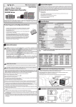
1
BoundT timing analysis tool User Guide TRUG001 Version 6.2 20080220 Tid rum Tidorum Ltd. Tid rum Tidorum Ltd www.tidorum.fi Tiirasaarentie 32 FI00200 Helsinki Finland This document, then a part of the BoundT User Manual, was written at Space Systems Finland Ltd by Niklas Holsti, Thomas Långbacka and Sami Saarinen. The document is currently maintained at Tidorum Ltd by Niklas Holsti. Copyright 2005 – 2008 Tidorum Ltd. This document can be copied and distributed freely, in any format or medium, provided that it is kept entire, with no deletions, insertions or changes, and that this copyright notice is included, prominently displayed, and made applicable to all copies. Document reference: Document issue: Document issue date: BoundT version: Last change included: Web location: TRUG001 Version 6.2 20080220 3 BTCH0106 http://www.boundt.com/userguide.pdf Trademarks: BoundT is a trademark of Tidorum Ltd. SPARC is a registered trademark of SPARC International, Inc. AVR and Atmel are registered trademarks of Atmel Corporation. Credits: This document was created with the free OpenOffice.org software, http://www.openoffice.org/. Preface The information in this document is believed to be complete and accurate when the document is issued. However, Tidorum Ltd. reserves the right to make future changes in the technical specifications of the product BoundT described here. For the most recent version of this document, please refer to the website http://www.tidorum.fi/. If you have comments or questions on this document or the product, they are welcome via electronic mail to the address [email protected] or via telephone or ordinary mail to the address given below. Please note that our office is located in the timezone GMT + 2 hours, and office hours are 9:00 16:00 local time. In summer daylight savings time makes the local time equal GMT + 3 hours. Cordially, Tidorum Ltd. Telephone: +358 (0) 40 563 9186 Web: http://www.tidorum.fi/ Email: [email protected] Mail: Tiirasaarentie 32 FI00200 Helsinki Finland Credits The BoundT tool was first developed by Space Systems Finland Ltd. (http://www.ssf.fi/) with support from the European Space Agency (ESA/ESTEC). Free software has played an important role; we are grateful to Ada Core Technology for the Gnat compiler, to William Pugh and his group at the University of Maryland for the Omega system, to Michel Berkelaar for the lpsolve program, to Mats Weber and EPFLDILGL for Ada component libraries, and to Ted Dennison for the OpenToken package. Callgraphs and flowgraphs from BoundT are displayed with the dot tool from AT&T Bell Laboratories. Some versions of BoundT emit XML data with the XML_EZ_Out package written by Marc Criley at McKae Technologies. iii Contents 1 INTRODUCTION 1.1 1.2 1.3 1.4 2 3 5 6 iv 37 Stacks and stack overflow.............................................................................37 Stack analysis to avoid stack overflow..........................................................40 Stack usage in loops......................................................................................41 Stack usage in calls.......................................................................................42 WRITING ANALYSABLE PROGRAMS 5.1 5.2 5.3 5.4 5.5 5.6 5.7 5.8 5.9 5.10 27 Introduction...................................................................................................27 Calls, call sites, and call paths.......................................................................28 Executions and contexts................................................................................29 Searching for the necessary context.............................................................31 Summary.......................................................................................................33 Examples.......................................................................................................34 Forcing context-dependent analysis..............................................................36 STACK USAGE ANALYSIS 4.1 4.2 4.3 4.4 6 Preliminaries....................................................................................................6 Installing Bound-T............................................................................................6 Running Bound-T.............................................................................................7 Easy examples : Loops....................................................................................8 Larger examples : Calls.................................................................................10 Drawing call-graphs and control-flow graphs................................................12 Harder examples : Assertions........................................................................18 What Bound-T can do....................................................................................20 What Bound-T cannot do...............................................................................21 Approximations..............................................................................................24 Getting started with a real program..............................................................25 CONTEXT-DEPENDENT ANALYSIS 3.1 3.2 3.3 3.4 3.5 3.6 3.7 4 What Bound-T is..............................................................................................1 Overview of this User Guide............................................................................3 Other Bound-T documentation........................................................................4 Typographic Conventions.................................................................................5 USING BOUND-T 2.1 2.2 2.3 2.4 2.5 2.6 2.7 2.8 2.9 2.10 2.11 1 51 Why and how.................................................................................................51 Count the loops.............................................................................................51 Simple steps and limits..................................................................................53 First degree formulas.....................................................................................53 Sign your variables........................................................................................54 Go native by bits...........................................................................................54 Aliasing, indirection, pointers........................................................................55 Switch to ifs...................................................................................................55 No pointing at functions................................................................................55 Final words.....................................................................................................56 GLOSSARY 57 Tables Table 1: Example of suffix contexts and full contexts.......................................................................30 Table 2: Stack space for max_freq on several processors..................................................................39 Table 3: Worstcase stack path for len_more on H8/300 with GCC..................................................47 Figures Figure 1: Inputs and outputs..............................................................................................................3 Figure 2: Flowgraph of sum_vector on SPARC................................................................................13 Figure 3: Flowgraph of sum_vector with SPARC instructions..........................................................15 Figure 4: Callgraph of sum_two on AVR..........................................................................................15 Figure 5: Boundsgraph drawing of sum_two on SPARC..................................................................17 Figure 6: Contextspecific flowgraphs for sum_vec_n on SPARC.....................................................18 Figure 7: Example of calls and call paths..........................................................................................29 Figure 8: Stack height profile...........................................................................................................43 Figure 9: Stack height and usage over a call.....................................................................................44 Figure 10: Stackusage profile of subprogram A...............................................................................45 Figure 11: Call graph of len_more and callees..................................................................................46 Figure 12: Stackusage profile (worst path) for len_more, H8/300, GCC........................................48 v This page is intentionally blank except for this note. vi 1 INTRODUCTION 1.1 What Bound-T is BoundT is a tool for developing realtime software computer programs that must run fast enough, without fail. The main function of BoundT is to compute an upper bound on the worstcase execution time (WCET) of a program or subprogram. The function, “bound time”, inspired the name “BoundT” pronounced as “bounty” or “bound tee”. Realtime deadlines A major difficulty in realtime programming is to verify that the program meets its runtime timing constraints, for example the maximum time allowed for reacting to interrupts, or to finish some computation. BoundT helps to answer questions such as • What is the maximum possible execution time of this interrupt handler? Is it less than the required response time? • How long does it take to filter a block of input data? Will it be ready before the output buffer is drained? To answer such questions, you can use BoundT to compute an upper bound on the execution time of the subprogram concerned. If the subprogram cannot be interrupted by other computations, and this upper bound is less or equal to the time allowed for the subprogram, we know for sure that the subprogram will always finish in time. When the program is concurrent (multithreaded), with several threads or tasks interrupting one another, the execution time bounds for each thread can be combined to verify the timing (schedulability) of the program as a whole. Such schedulability analysis is not a function of BoundT, but many schedulability analysis tools are available. Some tools are listed at http://www.tidorum.fi/boundt/schedulingtools.html. Static analysis all cases covered Timing constraints are traditionally addressed by measuring the execution time of a set of test cases. However, it is often hard to be sure that the case with the largest possible execution time is tested. In contrast, BoundT analyses the program code statically and considers all possible cases or paths of execution. BoundT bounds are sure to contain the worst case. Static analysis no hardware required Since BoundT analyses rather than executes the target program, targetprocessor hardware is not required. With the BoundT approach, timing constraints can be verified without complicated test harnesses, environment simulations or other tools that you would need for really running the target program. Of course, thorough softwaredevelopment processes should include testing, but with BoundT the timing can be verified early, before the full test environment becomes available. In many embeddedsystem development projects the hardware is not available until late in the project, but BoundT can be used as soon as some parts of the embedded target program are written. BoundT User Guide Introduction 1 It’s impossible, but we do it with assertions The task BoundT tries to solve is generally impossible to automate fully. Finding out how quickly the target program will finish is harder than finding out if it will ever finish – the famously unsolvable “halting problem”. For brevity and clarity, this manual generally omits to mention the possibility of unsolvable cases. So, when we say that BoundT will do such and such, it is always with the implied assumption that the problem is analysable and solvable with the algorithms currently implemented in BoundT. For difficult target programs, the user can control and support BoundT s automatic analysis by giving assertions. An assertion is a statement about the target program that the user knows to be true and that bounds some crucial aspect of the program's behaviour, for example the maximum number of a times a certain loop is repeated. Approximations Also bear in mind that BoundT produces an upper bound for the execution time, which may be different from the exact worstcase time. Various approximations in BoundT's analysis algorithms may give overestimated, too conservative bounds. However, the bounds can be sharpened by suitable assertions. These cautions and remedies are discussed in more detail later in this manual. Context and place Figure 1 below illustrates the context in which BoundT is used. The inputs are the compiled, linked executable target program, an optional file of assertions, and commandline arguments and options (not shown in the figure). The outputs are the bounds on execution time and stack usage (optional), as well as controlflow graphs and call graphs (also optional). Target program, target processor, target computer To use BoundT effectively, you must know the structure of the target program − the program being analysed. In some cases, you may have to understand the architecture of the target processor that will run the target program, and perhaps of the target computer – the computer that contains the target processor plus various peripherals, memories and other devices. BoundT is available for several target processors, with a specific version of BoundT for each processor. All BoundT versions are used in the same general way as explained in this User Guide. Additional information for specific targets is provided in separate BoundT Application Notes on which more below. Host computer The BoundT tool itself is installed and executed on a host computer – your PC or workstation. Since BoundT works entirely by static analysis, not by measurement or profiling, it needs no access to the target computer. You can use BoundT to analyse a target program before the target computer even exists, and before the target program is complete enough to be executed on the target computer. All you need is a crosscompiler and linker that can generate the machine code for the target processor. 2 Introduction BoundT User Guide Compiler & linker Source code User assertions on loop bounds, variable values, call counts, etc. BoundT Enter Foo() Main Foo Solve Count Ones Libraries Kernel Static analysis: Decode instructions Trace control flow Trace subprogram calls Find loop bounds Find worstcase path Main 9352 . Foo 121 . . Count 105 . Solve 9207 . . Count 303 . . Ones 721 Return Flow graphs Call graphs Execution time bounds Stack usage bounds Figure 1: Inputs and outputs 1.2 Overview of this User Guide What the reader should know This User Guide is intended to explain what BoundT can do and how BoundT is used. The reader is assumed to know how to program in some common procedural (imperative) language, such as C or Ada. Familiarity with realtime and embedded systems is an advantage. Most examples in the manual are presented in C, but BoundT is independent of the programming language, since it works on the executable machine code, not on the source code. BoundT User Guide Introduction 3 User Guide overview This document is a User Guide that introduces BoundT in a tutorial and informal way. The guide is organised into chapters as follows: 1.3 • Chapter 2 explains how BoundT is used. It introduces the basic methods, options and results for executiontime analysis. The nexttolast section tells how to get started with the analysis of a real program. • Chapter 3 gives more detail on contextdependent analysis, in which the execution time or stack usage of a subprogram can depend on actual parameter values or other context inherited from a particular chain of calls leading to that subprogram. • Chapter 4 covers the analysis of stack usage. Stack overflow can be fatal to embedded programs; stackusage analysis can make sure that overflow never happens. • Chapter 5 suggests how to write programs that BoundT can analyse. • Chapter 6 is a glossary of terms and concepts related to BoundT. Other Bound-T documentation This User Guide is not an exhaustive documentation of BoundT. It is supplemented by other documents as follows. Reference Manual For full and detailed information on commandline options and output formats, look to the BoundT Reference Manual at http://www.boundt.com/refmanual.pdf. The Reference Manual also outlines the analysis process and lists and explains the warning and error messages. Assertion Language manual Most users of BoundT need to write assertions to guide and constrain the analysis. Assertions are written as text. This User Guide gives several examples of assertions, but you should refer to the BoundT Asssertion Language manual at http://www.boundt.com/assertionlang.pdf for the full syntax and meaning of the assertion language. The possible warning and error messages from the assertion parser are also described there, not in this User Guide nor in the Reference Manual. Targetspecific Application Notes This User Guide, the Reference Manual, and the Assertion Language manual describe the general, targetindependent usage and features of BoundT. For specific target processors there are usually additional commandline options, perhaps additional forms of analysis and outputs, additional warning and error messages, and targetspecific aspects of the assertion language, such as the names of the processor registers. All of these are described in the BoundT Application Notes for your target processor at http://www.boundt.com/app_notes. 4 Introduction BoundT User Guide Languages, compilers, kernels BoundT is largely independent of the programming language and execution environment of the target program. When necessary, separate BoundT Application Notes advise on using BoundT with specific target languages, compilers, realtime kernels or target operating systems. Please refer to http://www.boundt.com/app_notes for the currently available Application Notes. Hard Real Time programming model BoundT contains special highlevel support for target programs that follow the HardRealTime (HRT) programming model, an architectural style for concurrent, realtime programs originally defined by the European Space Agency. For an HRT program, BoundT can generate socalled execution skeletons with detailed worst case executiontime information as required by HRT schedulability analysis. Using BoundT's HRT functions is quite optional. BoundT can be used for nonHRT applications without knowing anything about the HRT model and how BoundT supports this model. This User Guide describes how BoundT is used in its basic mode, without the special HRT features. There is a separate manual that explains how to use BoundT in HRT mode. See http://www.boundt.com/hrtmanual.pdf. 1.4 Typographic Conventions We use the following fonts and styles to show the role of pieces of the text in this guide: option A commandline option for BoundT. symbol A mathematical symbol or variable. text Text quoted from a source file or a command. keyword A keyword (reserved word) in a programming language or in the BoundT assertion language. BoundT User Guide Introduction 5 2 USING BOUND-T 2.1 Preliminaries BoundT is used as an additional tool in a software development environment. It is not a stand alone development tool, so you will need the usual kit of program editors, compilers and linkers to generate executable forms of your programs. To use BoundT, you need: 1. The target program for which execution time bounds are wanted. The program must be provided in an executable form, compiled and linked for the target processor. Source code for the target program is not absolutely necessary but makes it easier to control BoundT. 2. A version of BoundT that supports the specific target processor and executable file format (e.g. COFF or ELF) and runs on your host platform (e.g. Linux or MS Windows). 3. Usually, knowledge about the processing load of the targetprogram, such as the maximum size of data structures, is also required. If your linker produces a binary format that BoundT does not support, note that the freely available GNU tool objcopy, a component of the GNU binutils toolset, can be used to convert between various binary formats. If the target program is concurrent (multithreaded), a schedulinganalysis tool will also be useful, but is not required for using BoundT (nor is one included). Typical scheduling analysis tools use RateMonotonic Analysis (RMA) or DeadlineMonotonic Analysis. 2.2 Installing Bound-T Host and target computers This section explains briefly and in general how to install BoundT on your computer. The computer on which BoundT is installed and used is known as the host computer. It is usually not the same as the target computer on which the target program runs or will run. The host and target computers usually have different types of processor, for example a powerful RISC processor on the host computer and a small 8bit microcontroller on the target. Note that you do not need to have a target computer available in order to use BoundT, and even if you have one it does not need to be connected to your host computer. BoundT works purely by static analysis of the machine code of the target program, and this static analysis is done by running BoundT on the host computer. BoundT does not use any form of measurement or execution of the target program on the target computer itself. Delivery medium and specific instructions Specific installation instructions for each supported type of host computer and host operating system are included with each delivery of BoundT, on the delivery medium or as hardcopy enclosed with the medium. On a typical host computer, an installation of BoundT for one target processor consists of a bin directory folder with three executable programs: BoundT itself and two auxiliary programs. On Unixlike platforms the folder also contains two short executable shellscripts that assist the auxiliary programs. 6 Using BoundT BoundT User Guide Support for each additional target processor type adds one executable of BoundT itself to the bin folder. The auxiliary programs are the same for all targets. The main steps in the installation are to copy the bin folder to the host computer and to set up the PATH variable, or an equivalent mechanism, to make the contents of bin available on the command line. The dot program for handling the graphical output is not included on the delivery medium. Install it from http://www.graphviz.org. Disk space requirements The disk space consumed by BoundT depends on the host computer but allowing 30 MB should be ample for one type of target processor. Each additional target processor type needs about 15 MB more disk space. Processor and memory requirements BoundT usually places about the same demands on the host computer's processor speed and memory size as a typical compiler does. For complex target programs the arithmetic analysis of loopbounds may require a great deal of time and memory. However, experience shows that a normal desktop PC can handle many arithmetic analysis problems, and the larger problems are better dealt with by asserting loop bounds manually, or by simplifying the target program. Hostspecific usage instructions Advice on using BoundT on various host computers, when necessary, is given in separate host specific Application Notes included on the installation medium or enclosed as hardcopy. Verifying the installation The installation instructions and host notes show how to get started by using BoundT on examples provided with the installation. These examples are sufficient to verify that all components of BoundT are functional. 2.3 Running Bound-T BoundT is started with a command of the form boundt <options> <target exe file> <subprogram names> This command requests BoundT to compute upper bounds for the worstcase execution time and/or the stack usage of the named subprograms within the given executable target program file. The Reference Manual describes all the commandline options, but you will see several examples later in this guide. This computation can either succeed fully automatically, or succeed only after some additional assertions are given. The Assertion Language manual describes the full assertion language, but there are several examples in this guide. For an HRToriented analysis, BoundT is started with a command of the form boundt hrt <more options> <target exe file> <TPOF name> BoundT User Guide Using BoundT 7 See section 1.3 for more about the HRT analysis mode. The command name, written just boundt above, usually includes a suffix to indicate the target processor, for example boundt_avr names the BoundT version for the Atmel AVR processor. Please refer to the relevant Application Note for the exact name. When you install BoundT you can also change the name, or define an alias or abbreviation for it. 2.4 Easy examples : Loops At last, some code! To show what BoundT can do, consider the following C function that computes the sum of the elements of a vector of floatingpoint numbers: #define VECTOR_LENGTH 100 float sum_vector (float vector[]) { int i; float sum; sum = 0.0; for (i = 0; i < VECTOR_LENGTH; i++) sum += vector[i]; return sum; } Assume that this function is stored in the file sum.c and compiled and linked (together with some main function, not shown) into an executable program called summer.exe. Then, the BoundT command boundt summer.exe sum_vector will display an upper bound on the worstcase execution time (WCET) of sum_vector as the last field of the output line: Wcet:summer.exe:sum.c:sum_vector:48:1103 The WCET is given as the number of instruction cycles (1103 in this example, when the function is compiled for the SPARC ERC32 processor). The corresponding number of seconds or microseconds of real time depends on the particular target processor and its clock frequency, as explained in the Application Note for this processor. The numbers in the preceding field, 4 – 8, are the sourcecode linenumbers of the subprogram. BoundT gets these linenumbers from the compilergenerated mapping between code addresses and sourcecode lines, which often leads to a little fuzziness, for example by omitting the line numbers for syntactical brackets like the '{' and '}' that enclose the body of the function. How did it do that? How does BoundT compute the worstcase execution time? To use BoundT effectively, it helps to know the general method, although it is not necessary to understand the details. 8 Loop examples BoundT User Guide First, BoundT reads in the executable program and uses the symbolic debugging information to find the entry point of the code of the sum_vector function. Then, BoundT decodes the machine instructions to generate the controlflow graph of sum_vector and to locate the loop. BoundT analyses the arithmetic of the looping code and infers that the loop is executed 100 times. BoundT reports this by printing Loop_Bound:summer.exe:sum.c:sum_vector:78:99 (The loopbound is reported as 99 instead of 100 because BoundT computes the number of times the looping code goes back to the start of the loop.) This defines the exact sequence of machine instructions that are executed in a call of sum_vector, and BoundT simply adds up their execution time to give the WCET. How does it know the execution time of the instructions? For simple target processors each type of instruction has a fixed execution time − so many clock ticks. Sometimes the execution time depends on the sort of operands the instruction uses, for example memory operands taking longer than register operands, and BoundT takes this into account. On pipelined processors the execution time can depend on what other instructions are in the pipeline. BoundT models the pipeline state to include this effect. For some complex instructions, such as multiplication, division or floating point instructions, the execution time can vary depending on the values of the operands − the numbers being multiplied, for example. BoundT usually assumes a worstcase execution time for such instructions. Some target processors have several kinds of memory, at different memory addresses and with different access times. For example, onchip memory is usually faster than offchip external memory. For such processors, BoundT analyses the address in each memoryaccessing instruction to find the memory areas it can access and thus the access time. If the memory area remains unknown, BoundT uses the access time for the slowest type of memory. Some target processors have cache memory or branch prediction units or other types of acceleration mechanisms that store execution history and have a large effect on instruction execution time. Some target processors have several internal functional units that work in parallel, more or less asynchronously, also affecting the execution time. In its present form, BoundT does not support such target processors. Syntax is only sugar Since BoundT works on the binary, executable code and not on the source code, it's not picky about the way loops are written: forloops, whileloops, dowhileloops or even gotoloops are all acceptable, as long as the loop is counterbased. For example, here is sum_vector with a do whileloop: #define VECTOR_LENGTH 100 float sum_vector (float vector[]) { int i = 0; float sum = 0.0; do { sum += vector[i]; } while (++i < VECTOR_LENGTH); return sum; } BoundT User Guide Loop examples 9 Goto is not harmful Not only can loops be written with the goto statement, but the goto can also be used in other ways, for example to exit from a loop in the middle. The same holds for other controlflow statements such as the C statements continue and break and the Ada exit statement. Any control structures in the programming language can be used, as long as the loops are counterbased and nicely nested within each other (in technical terms, the controlflow graph must be reducible). 2.5 Larger examples : Calls The root calls its children In the above examples, the target subprogram did not call any other subprograms. Such calls are of course allowed, and BoundT will automatically analyse the call graph and compute WCET bounds for all called subprograms, and finally for the “root” subprograms named on the command line. If the WCET of a subprogram depends on the actual value of a parameter, BoundT tries to compute the WCET separately for each call of a subprogram. This can extend progressively to calls within this call, and so on, as will be explained in Chapter 3. An example follows. What if vectorlength is a parameter? A flexible vectorsumming function should have the vectorlength as a parameter, for example called n: float sum_vec_n (float *vector, int n) { int i; float sum; sum = 0.0; for (i = 0; i < n; i++) sum += vector[i]; return sum; } Now the command boundt summer.exe sum_vec_n will report that sum_vec_n “could not be fully bounded”. The reason is that BoundT found no (reasonable) upper bound on the loopcounter i, because there is no (reasonable) upper bound on the parameter n. BoundT points to the source of the problem as follows: sum_vec_n Loop unbounded at sum.c:1718, offset 00000014 However, when the target program calls the sum_vec_n function, the call gives an actual value for the parameter, for example thus: float sum_two (void) { 10 Call examples BoundT User Guide float v1[40], v2[1234]; float sum1, sum2; ... sum1 = sum_vec_n (v1, 40); sum2 = sum_vec_n (v2, 1234); ... return sum1 + sum2; } If the above function is stored in sum_two.c, then compiled and linked into summer.exe, the command boundt summer.exe sum_two will compute a WCET bound, for example: Wcet:summer.exe:sum_two.c:sum_two:412:9119 Although BoundT again failed to bound the loop in sum_vec_n as such, it repeated the analysis for each of the two calls of sum_vec_n in sum_two. With n known to be 40 or 1234, respectively, BoundT could compute loopbounds and WCET for each call and thus also the total WCET for sum_two. Chapter 3 explains how such contextdependent analysis works in more detail. The results for each call are reported in the following form: Loop_Bound:summer.exe:sum.c:sum_two@8=>sum_vec_n:1718:39 Loop_Bound:summer.exe:sum.c:sum_two@9=>sum_vec_n:1718:1233 Wcet_Call:summer.exe:sum.c:sum_two@8=>sum_vec_n:1418:445 Wcet_Call:summer.exe:sum.c:sum_two@9=>sum_vec_n:1418:8647 The fourth colondelimited field shows the callpath context for each result. For example, the first Loop_Bound is valid when sum_vec_n is called from sum_two at line 8 of sum.c, while the second Loop_Bound is valid for the call from line 9. Loops within loops Nested loops are handled in the same fashion, for example: float sum_matrix (float *matrix[], int m, int n) { int i, j; float sum; sum = 0.0; for (i = 0; i < m; i++) { for (j = 0; j < n; j++) sum += (matrix[i])[j]; } return sum; } Since the looplimits m and n are again parameters, BoundT cannot compute a WCET for this subprogram as such. Once m and n are given values in a call of sum_matrix, the WCET can be computed just as in the earlier example with sum_vec_n. BoundT User Guide Call examples 11 2.6 Drawing call-graphs and control-flow graphs DOT drawings BoundT does not have a graphical user interface, but it can draw the callgraph and the controlflow graphs of the subprograms that are analysed. The graphs are generated as output files that describe the structure of the graphs for the DOT tool. The DOT tool is a part of the GraphViz suite that you can download from http://www.graphviz.org/. The DOT tool reads the graph structure file, decides how to lay out the nodes, edges, and labels in a twodimensional drawing, and generates the drawing in some graphical file format, for example PDF or JPEG. You can then view the drawings using a tool such as Acrobat Reader for PDF files. The DOT description of a graph is in text form. You can make small tweaks to the graphs by simple text editing, for example to change from portrait format to landscape format. Commandline options for graph drawing To make BoundT draw callgraphs or flowgraphs, you must • use the option dot or the option dot_dir to say where the drawings go, and • use some draw options to say what the drawings should show. The dot option puts all drawings into one file. You write the name of this file after the dot, separated by whitespace (so it becomes the next argument on the command line). For example, the following command (where the ... stands for more options and arguments) puts all the drawings (all the DOT text) into the file graphs.dot: boundt dot graphs.dot draw ... The dot_dir option puts each drawing in a separate file of DOT text, and puts these files in one directory folder. You write the name of the directory folder after the dot_dir, separated by whitespace. For example, the following command puts each drawing into its own file in the directory graphdir: boundt dot_dir graphdir draw ... With dot_dir, BoundT names the drawing files automatically as explained in the Reference Manual. The names of callgraph drawings start with “cg_” and the names of flowgraph drawings start with “fg_”. BoundT tries to include the name of the relevant subprogram in the name of the drawing file, but it may have to remove or change special characters into ordinary letters in the filename, so don't expect a perfect match for all names. The draw option is followed by a keyword that selects or excludes a particular form of drawing or particular information that may be present in a drawing. The Reference Manual explains the draw options fully; here we focus on examples. The most common use of draw options is probably the simple form draw total which draws the callgraph in the default form (each subprogram seen as one node) and one flowgraph for each analysed subprogram, giving the total number of executions and the total execution time for each basic block in each subprogram. 12 Drawing graphs BoundT User Guide First example: sum_vector For a first example of controlflow graphs, take the subprogram sum_vector from section 2.4 (page 8). Add the dot and draw options to the BoundT command: boundt dot grf.dot draw total summer.exe sum_vector This command puts the callgraph diagram and the flowgraph diagram in the file grf.dot. You can then convert this file to a PostScript file, for example, with the DOT command: dot Tps <grf.dot >grf.ps Assume, for example, that sum_vector is compiled for the SPARC processor. In this case the call graph is trivial because sum_vector calls no other subprograms. Figure 2 below shows the drawing of the flowgraph of sum_vector from this analysis. Figure 2: Flow-graph of sum_vector on SPARC The flow of execution in flowgraph drawings is mostly topdown. The entry point is identified by the entry arrow at the top, labelled to show how many calls of the subprogram are included in the total (because this drawing comes from draw total, remember). The rectangular nodes are the basic blocks and are labelled with the sourcecode lines that correspond to each instruction in the block. The last two lines in the nodelabel show the execution count and execution time of the node. For example, the first node (the entry point) in Figure 2 is executed once (“count 1”) and takes 4 cycles to execute (“time 4”). BoundT User Guide Drawing graphs 13 The edges (arcs) represent flow of execution from one node to another, in the direction of the arrowhead. Edges are labelled with the execution count and with the execution time (if not zero). The edges on the worstcase execution path are drawn with a greater thickness (bolder) than other edges. In Figure 2, however, all edges are on the worstcase execution path. The second node and the lowermost node on the left side of Figure 2 represent the loop in sum_vector. The node that forms the loop head is labelled with the loop number (“loop #1”). The “count” labels show that the loop head is executed 100 times while the other node in the loop is executed only 99 times. For nodes and edges that are executed more than once the “time” labels show two numbers separated by a semicolon. The first number is the time for one execution; the second number is the total time for all executions. For example, the edge that returns to the loop head from the other node in the loop is labelled “time 4; 396” meaning that one execution of the edge can take up to 4 cycles, so the 99 executions take up to 4 99 = 396 cycles in total. (As an aside, this edge has such a large time, 4 cycles, because it is a short path from one SPARC floating point addition instruction to another such instruction, which may force the program to wait for the SPARC floatingpoint unit to complete the first instruction.) The lowermost node on the righthand side of Figure 2 is reached when the loop terminates. There is no edge out from this node, so the subprogram returns after executing this node. Disassembled code in the flowgraph The following draw options will show the disassembled machine instructions, instead of the sourcecode lines, in the flowgraph: boundt dot grf.dot draw total draw decode draw cond draw no_line draw no_count draw no_time summer.exe sum_vector The resulting flowgraph drawing for sum_vector on a SPARC is shown in Figure 3 below. Compared to Figure 2, the sourceline references are removed (draw no_line) and so are the execution counts and times (draw no_count and draw no_time) and instead (draw decode) the drawing shows the disassembled SPARC instructions, one per line, in execution order, with the address of each instruction in the left margin. Thanks to draw cond the edges are labelled with the logical condition for taking the edge, which is true for unconditional edges and otherwise some logical formula using the Z (zero) and N (negative) condition flags from the SPARC status register. Call graph of sum_two Consider again the subprogram sub_two from section 2.5 (page 10). The following command makes BoundT analyse it and draw the callgraph and controlflow graphs: boundt dot grf.dot draw total summer.exe sum_two The callgraph is no longer trivial because sum_two calls sum_vec_n (twice, in fact). If the program is compiled for the Atmel AVR processor, the callgraph looks even more interesting, as Figure 4 below shows. The AVR has no hardware floatingpoint unit, so the compilers instead use library routines to implement floatingpoint operations. In this example, both sum_two and sum_vec_n call the library routine for floatingpoint addition, ?F_ADD_L04, which is not visible at all in the source code of this program in section 2.5. This library routine in turn calls three other library routines: ?TEST_P_L04 and two anonymous routines that BoundT identifies with their entry addresses, 0000E2 and 00002E hex. 14 Drawing graphs BoundT User Guide Figure 3: Flow-graph of sum_vector with SPARC instructions Figure 4: Call-graph of sum_two on AVR BoundT User Guide Drawing graphs 15 The nodes (rectangles) in the callgraph represent subprograms. The root subprogram, sum_two in this example, is on the top. The node label gives the name of the subprogram, the number of calls of this subprogram that are executed on the worstcase execution path, the number of different callpaths that can lead to these calls, and the total time (upper bound) of these executions. For example, Figure 4 shows that sum_two is executed once (“one call”) from one call path, which is always and naturally the case for the root subprogram. Furthermore, the total time is the WCET bound for sum_two, 865 909 AVR clock cycles (“time 865909”). The last line in the label for a subprogram shows the division of the total execution into time spent in the subprogram itself (“self”) and time spent in other subprograms that are called from this subprogram (“callees”). For sum_two only 93 cycles of the total time is spent in sum_two itself, the rest being spent in the callees: sum_vec_n and the floatingpoint routines. Looking at the lower levels of the callgraph, the library routine ?F_ADD_L04 is called (executed) 1275 times, along three call paths: firstly, from sum_two directly; secondly, from sum_two via the first call of sum_vec_n; and thirdly, from sum_two via the second call of sum_vec_n. When a subprogram is executed more than once, the “time” label shows how the total time is the product of the number of executions and the time per execution. Thus, the “time” label for ?F_ADD_L04 shows that the total time, 826 200 cycles, equals the product of 1275 executions and the time per one execution, 648 cycles. Here each execution of ?F_ADD_L04 is given the same, contextindependent, execution time bound; in reality, however, the execution time of this subprogram depends on the values of the floatingpoint numbers to be added. For a subprogram that has contextspecific bounds, the time per execution is shown as a range min .. max. For example, the “time” label for sum_vec_n shows that the total time, 865 168 cycles, comes from 2 executions where the time per execution ranges from 27 221 cycles to 837 947 cycles. The edges (arcs) in the callgraph represent calls (callercallee relationships). They point from the caller subprogram to the callee subprogram. The edge labels show the number of call paths and the execution time bounds. Drawing contextdependent execution bounds: the bounds graph For suprograms with contextdependent executiontime bounds, such as sum_vec_n, you may like to draw a graph that is like a callgraph but separates the different execution bounds. Use the option draw bounds to create such “boundsgraph” drawings. For example: boundt dot grf.dot draw bounds summer.exe sum_two This command makes a boundsgraph drawing in the file grf.dot. It makes no callgraph drawing (because callgraph and boundsgraph drawings are mutually exclusive options) and no flowgraph drawings (because the command has no draw option for them). Figure 5 below shows the boundsgraph drawing for sum_two on the SPARC target processor. A callgraph drawing would show sum_vec_n once, covering both calls of this subprogram and showing a range of executiontime bounds, 445 .. 8647 cycles. In contrast, the boundsgraph drawing in Figure 5 shows the two calls separately, because they have different bounds on execution time. 16 Drawing graphs BoundT User Guide Figure 5: Bounds-graph drawing of sum_two on SPARC Drawing contextdependent flowgraphs The earlier examples of flowgraph drawings all use the option draw total which, for each subprogram, creates a single flowgraph drawing that summarises all executions of that subprogram on the analysed worstcase path for the root subprogram. For subprograms with contextdependent executiontime bounds, such as sum_vec_n, you may like to draw a separate flowgraph for each context or for chosen contexts. BoundT provides six different draw options to choose which flowgraphs to draw. The earlier examples in this section used draw total; the example below uses draw all; the Reference Manual explains the other four options. Use the option draw all to make a separate flowgraph drawing for each context in which a subprogram has been analysed and given contextspecific execution bounds. For example: boundt dot grf.dot draw all summer.exe sum_two This command makes a callgraph drawing in the usual form and then makes flowgraph drawings for each subprogram in all contexts. For this example, on the SPARC processor, the only subprogram with contextspecific bounds is sum_vec_n, which has two bounds corres ponding to the two calls of this subprogram from sum_two. Figure 6 below shows the resulting two flowgraph drawings, side by side. In this example, the only difference between the two flowgraph drawings in Figure 6 is the indication of the callpath, given at the very top and showing that the calls lie on different lines (numbers 8 and 9) in sum_two, and the execution counts of nodes and edges in the loop, reflecting the different value of the parameter n in the two calls. You may wonder why Figure 6 shows that sum_vec_n has an execution path that bypasses the loop entirely, going from the entry node via another node to the return node. There is no if statement in the sourcecode (page 10) that could make the loop conditional. However, the number of loop iterations depends on the parameter n, which may be zero or negative, in which case the loop should not be executed at all. The compiler inserts a test and branch for this case because the compiler can then generate a bottomtest loop body (do until) instead of a toptest (while do). Since the actual value of n in both contexts is positive, this bypass path is not on the worstcase path and therefore shows zero execution counts in Figure 6 and the edges on the bypass path are drawn as thin lines. BoundT User Guide Drawing graphs 17 Figure 6: Context-specific flow-graphs for sum_vec_n on SPARC 2.7 Harder examples : Assertions Whileloops may be confusing Next, consider the more complex C function binary_search that looks up a value in a sorted vector using a divideandconquer approach: int binary_search (int *vector, int val) { int low, high, mid; low = 0; high = VECTOR_LENGTH 1; while (low <= high) { mid = low + (high low) / 2; if (vector[mid] == val) return mid; else if (vector[mid] < val) low = mid + 1; else high = mid 1; } 18 Assertion examples BoundT User Guide return 1; } If this function is stored in the file bins.c and compiled and linked into the executable program file bins, the BoundT command boundt bins binary_search reports that the subprogram could not be fully bounded because no bounds were found for the whileloop. When BoundT analysed the control and data flow of binary_search, it could not find any variables that act as loop counters with simple initial and final values and simple increments. For a nontrivial algorithm such as binary search this is not very surprising. Assertions make it clear What can be done to work around this problem? The BoundT user must help out by telling BoundT the maximum number of times the loop can repeat. This is done with an assertion placed in a separate assertion file. The Assertion Language manual explain this fully, but here is how to do it in this example. Assuming that VECTOR_LENGTH is 100, the maximum number of iterations is 7. The assertion takes the form subprogram "binary_search" loop repeats <= 7 times; end loop; end "binary_search"; If this assertion is placed in a file prog.bta and BoundT is run with the command boundt assert prog.bta bins binary_search the analysis succeeds and BoundT displays the WCET bound, for example as Wcet:bins:bins.c:binary_search:418:129 Counters make it clear, too Another way to help BoundT find bounds on loops is to add loopcounters when there are none to start with. For example, the binary_search function could be changed as follows: int count = 0; ... while (low <= high) { mid = low + (high low) / 2; ... count += 1; if (count > 7) break; } Now the looprepeat condition contains an explicit limit on a counter value, and BoundT can compute a WCET bound without any help from assertions. The limit can be made a parameter of the subprogram, of course, instead of a constant (7) as in this example. BoundT User Guide Assertion examples 19 Eternal loops take a little longer Much has been said about finding bounds on the number of iterations of loops. But what if the program contains an eternal loop? We call a loop eternal if it cannot possibly terminate, either because there is no instruction that could branch out of the loop, or because all such branch instructions are conditional and the condition has been analysed as infeasible (always false). Obviously, the execution time of a subprogram that enters an eternal loop is unbounded. Nevertheless, since realtime, embedded programs are usually designed to be nonterminating, they usually contain eternal loops. To analyse the execution time of an eternal loop you must assert an assumed number of repetitions of the loop. The Assertion Language manual has more to say on eternal loops. 2.8 What Bound-T can do This section outlines BoundT's current abilities, which are, of course, constantly being extended. This is generic information, applicable to all target processors. Targetspecific Application Notes define more precisely BoundT's abilities and limits for each target. Control flow tracing BoundT can decode all target processor instructions. BoundT can analyse the controlflow and callgraph of any subprogram that follows the processor's calling standard and where the destination addresses of each branch are statically defined in the code. For normal branches, which the compiler generates for conditional or looping statements, or for calls that give the real name of the callee, the destination address is usually an immediate literal in the branch instruction, and so is statically defined. Note that for a conditional branch, although the possible destinations must be known statically, the condition (boolean expression) that selects the actual destination can be dynamically computed at runtime, and usually is. Switches and cases Large and dense switchcase statements often use a simple form of dynamic destination addressing in which the caseselector is used as an index to a table that gives the starting address of the corresponding branch of the switchcase statement. BoundT contains specific dataflow analysis to derive static bounds on the value of the caseselector and thus find the caseaddress table and the possible destinations of such a branch. However, the current version of BoundT is limited in the kind of switchcase code it can analyse. Refer to the Application Notes for particular target processors and target compilers for details. Counterbased loops As the two examples earlier in this chapter showed, sometimes BoundT can analyse the target subprogram well enough to arrive at a WCET bound automatically, but sometimes the user must provide assertions to guide and constrain the analysis. The most important factor that decides the need for user assertions is the complexity of the looptermination conditions. 20 What BoundT can do BoundT User Guide The dataflow and loopanalysis algorithms currently implemented in BoundT are designed to handle counterbased loops automatically. A counterbased loop is a loop that always increments (or decrements) a counter variable on each iteration, and terminates when the counter becomes greater than (or less than) a limit. It is not necessary that a counterbased loop is actually written as a forloop in the target program source code; what matters is the way the logical exit condition is written, and the way the counter variable is updated. The counter's step (increment or decrement) can be positive or negative, but it must have the same sign for all loop iterations. The absolute value of the step can vary from one iteration to another, as long its lower bound is nonzero. The initial and final values of the counter need not be known exactly; as long as they are bounded in suitable directions, BoundT will compute the worstcase number of loop iterations, using the value of the step that has minimum absolute value, and those extreme values of the initial and final values that are farthest from each other. To determine a loopcounter's initial value, step, and limit value, BoundT can follow any computation in the target program that uses integer addition, subtraction and multiplication by a constant. Values of parameters are propagated into calls, but not in the other direction (from callees to callers). When BoundT stumbles As already said, deducing the worstcase execution time of an arbitrary program is unsolvable in principle, so any tool like BoundT must fail when the target program is complex enough. When BoundT cannot handle a problem automatically, it is usually possible to write assertions that let BoundT solve the problem. Of course, in this case the validity of BoundT's results depends on the validity of the assertions, which is the user's responsibility. An alternative solution is to change the target program to make it easier to analyse. For example, if the target program contains a whileloop that BoundT cannot find bounds for, simply adding an iteration counter and limit to the loop will solve the problem (and perhaps make the target program more robust, too). Chapter 5 advises on programming styles that help BoundT analyse the program. 2.9 What Bound-T cannot do The analysis algorithms in BoundT have been chosen and tuned to handle many forms of loops and other program structures automatically. However, sometimes the target program is too complex or inscrutable for these algorithms. Here is a list of things BoundT cannot currently do, ordered approximately from the most common to the least common problems. Fortunately, most problems can be worked around as explained below. Uncounted loops BoundT cannot infer the maximum number of loop repetitions for loops that do not have explicit counters and limits on the counters. As in the examples in section 2.7, this can be worked around with assertions or with sourcecode changes. BoundT User Guide What BoundT cannot do 21 Multiplication, division etc The method BoundT uses to analyse the loopcounter computations handles only addition and subtraction of variables and multiplication by constants. If the computation of a loopcounter's initial value, step or limitvalue involves any arithmetic operation beyond this, such as the multiplication of two variables, the value may become “unknown” to BoundT. The same workarounds apply as for loops without explicit counters. Multipleprecision arithmetic BoundT bases its analysis on a model of the native instructions in the target processor, using the native number of bits per value (word length). For processors with a small word length, such as 8 bits, the compiler (or assemblylanguage programmer) has to construct wider arithmetic from two or more 8bit parts and two or more 8bit instructions connected by some form of carry flag. BoundT usually does not model such multipleprecision arithmetic which means that it usually cannot bound loops that use multipleprecision counters, for example 16 bit counters on an 8bit machine. The targetspecific Application Notes explain the types of arithmetic instructions and operands that BoundT supports for the target processor. Aliasing and pointer chasing If a variable is not directly assigned within a loop, BoundT assumes that it is unchanged (invariant) throughout the loop. This assumption may be wrong if the variable is accessed indirectly through pointers, that is, via a memory reference with a dynamically computed address. The pointeraccess may be explicit in the source program, or it can result from implicit aliasing between parameters that are callbyreference. BoundT records which global variables (including processor registers) are directly assigned in each subprogram. Each call of the subprogram is then considered to assign unknown values to these global variables, which is important if the call is in a loop that uses this global variable in its loopcounter computation. However, if the called subprogram assigns the global variable via a pointer, BoundT does not include the assignment in the analysis of the loopcounter arithmetic, which may lead to wrong results. Although BoundT has an option (warn access) to emit a warning messages for all dynamic, indirect memory accesses that it cannot resolve, most of these are just array accesses and are usually irrelevant to loop counters. Thus, with the present version of BoundT, the user is responsible for avoiding aliasing that could distort the analysis of loop bounds. Overflow in the target program The method BoundT uses to analyse the loopcounter computations assumes that these computations do not overflow when the target program is executed. If overflow occurs, the bounds computed by BoundT may be incorrect, or BoundT may fail to find bounds at all. Note that this refers to overflow in some future execution of the target program, not to overflow in BoundT's own computations, which are checked against overflow. We believe that the auxiliary tools, oc and lp_solve, also contain internal overflow checking. The only workaround is to change the target program to guard against overflow, and to not use overflow on purpose in loopcounter computations. It is feasible to extend BoundT to consider overflow, and we are studying how to do it efficiently. 22 What BoundT cannot do BoundT User Guide Unsigned arithmetic The method BoundT uses to analyse the loopcounter computations assumes that the variables can take both positive and negative values and that there are no “wraparound” effects from unsigned arithmetic. For example, in common programming languages decrementing an unsigned integer variable that has the value zero gives a large positive value of the form 2n – 1 and not the value –1. Such wraparounds are similar to overflow and are currently not handled by BoundT. Usually, the workaround is to use only signed variables and signed arithmetic instructions in the target program's loop counters. However, check with the Application Note for the target processor as there may be targetspecific solutions. It is quite feasible to extend BoundT to include unsigned arithmetic and this is planned for future versions. It may already be implemented for specific target processors; again, please check the Application Note for your target. Jumps and calls via pointers Except for some switchcase statements and some locally dynamic calls, BoundT cannot handle a branch to an address that is not known until runtime. The most common cause of such dynamic branches is calling a subprogram via a pointer. This restriction also excludes objectoriented programming with dynamically bound methods such as C++ virtual functions. (Except that some C++ compilers do store enough information in the executable file about the class hierarchy and virtual functions for BoundT to discover all possible targets of a given virtual function call.) When BoundT finds a dynamic call that it cannot resolve, it issues an error message and handles the call as if it took no time and had no effect. If you know which subprograms can actually be called by this call, you can give BoundT this information as an assertion, or you can use BoundT to find the maximum WCET of these potential callees and add it to the WCET that BoundT reports for the caller. When BoundT finds a dynamic jump that it cannot resolve, it issues an error message and handles the jump as if it were a return instruction. That is, the WCET reported for the subprogram that contains the jump does not include the execution after the jump. If you know the possible targets of the jump, you may be able to use BoundT to find the maximum WCET of the code after the jump and add it to the WCET that BoundT reports for the subprogram that contains the jump. However, it is probably easier to change the target program to get rid of the dynamic jump. For dynamic calls and jumps, the closest alternative program structure is to write a switchcase statement or a nest of ifthenelse statements in which the various branches contain static calls or jumps to all the possible callees or jump targets. Exceptions and traps Many target processors and some programming languages perform automatic runtime checks on the computation, for example for numerical errors such as division by zero or for logical errors such as array index out of bounds. When a check fails the normal program flow is interrupted and execution continues at the address of the handler routine for the exception or trap. Execution may or may not return to the original program flow. Obviously this changes the execution time, perhaps radically. There are basically two kinds of traps: hardware traps and software traps. For hardware traps the check and possible branch to a trap handler are an implicit part of normal instructions. For example, the processor could be designed so that all addition instructions check and trap on overflow. BoundT User Guide What BoundT cannot do 23 For software traps the check or the branch to the trap handler are programmed by specific instructions. For example, most processors are designed to that an addition overflow just sets an overflow flag. To take an overflow trap the addition instruction must be followed by a conditional branch instruction that branches to the trap handler if the overflow flag is set. BoundT generally assumes that no hardware traps occur in the execution under analysis. Thus, the WCET bound does not include hardware traps. Software traps, in contrast, appear to BoundT as normal program flow and are thus included in the analysis. However, the address of the trap handler is usually not given statically but in some kind of “trap table” or “vector table” which means that the trap handler is located via a pointer and BoundT may be unable to find the handler for analysis. Irreducible flow graphs BoundT can analyse loops only in controlflow graphs that are reducible. A reducible control flow graph is one in which each loop is entered at a single point and any two loops are either nested one within the other or are entirely separate (no shared instructions). It is commonly observed that nearly all programs are reducible in the source code form, but sometimes the compilers emit irreducible object code, perhaps due to optimisation. Assemblylanguage subprograms such as runtime library routines are sometimes also irreducible, perhaps due to manual optimisation. When a subprogram has an irreducible flowgraph BoundT cannot find the loop structure. Thus, it cannot find loop repetition bounds by analysis and cannot accept assertions on loop repetition bounds. This does not hamper stack usage analysis, but it does pose a problem for executiontime analysis. There is a workaround, however. If the repeated execution paths in an irreducible flowgraph always pass through calls, and if you can assert bounds on how many times each such call can be repeated, then BoundT may be able to compute executiontime bounds even in the absence of a reducible loop structure. However, you must specifically tell BoundT to attempt this, by asserting that the assertions on the calls are enough for time. Refer to the Assertion Language manual for details. Recursion BoundT cannot analyse recursive calls. BoundT builds WCET bounds in a bottomup way from the lowestlevel subprograms (leaf subprograms) towards higherlevel subprograms (root subprograms). If the subprograms are recursive this bottomup method does not work and BoundT reports an error. However, you can analyse recursive programs by using assertions to slice the call graphs into nonrecursive parts. The method is explained the Assertion Language manual. 2.10 Approximations When BoundT computes upper bounds on worstcase execution time, it uses three types of approximation, corresponding to three sources of unknown variation in execution time. Instructionlevel approximations The execution time of some instructions in the target processor may be inherently variable. For example, the time can depend on the data being processed, or on the history of recently executed instructions and memory accesses. For each instruction BoundT uses an upper bound 24 Approximations BoundT User Guide on the execution time that takes into account some of this variation for the context of this instruction. The details depend on the target processor but in general the analysis includes pipeline effects but not cache effects. Although these dynamic features are increasing strongly in highend processors, many smaller, embedded processors are still quite deterministic, with fixed instructionexecution times. The Application Note for a particular target processor will describe the instructionlevel approximations in detail. Loopcount approximations The bounds on loop iterations computed by BoundT are upper bounds. Early exits (breaks) from loops can make the real number of iterations smaller. A similar approximation occurs for “nonrectangular” nested loops where the limits of the inner loop depend on the index of the outer loop. A typical example is a pair of loops that process the upper (or lower) triangle of an N×N square matrix. Here the current version of BoundT can only give, automatically, an N 2 bound on the number of executions of the inner loopbody. However, the real bound, N(N+1)/2, can be asserted, if the inner loopbody contains a feature that can be used to identify it. Feasible path approximations In a sequence of conditional statements, loops or other control structures, the several conditional expressions are sometimes correlated so that only a subset of paths can actually occur. For example, this happens if a conditional of the form “if A” is followed by a conditional of the form “if not A”, where the value of A is unchanged. BoundT is generally not able to correlate the conditions, but will compute the WCET over all apparently possible paths, allowing any combination of condition values, including logically impossible combinations. If the branches have very different execution times, a considerable overestimate in WCET can result. In some cases the approximation can be corrected with assertions. For example, if the code is in a loop, and the branches can be identified by some of their features (such as the calls they contain), one can assert an executioncount bound on certain branches that is less than the number of iterations of the loop. This forces BoundT to “bypass” these branches for a selectable fraction of the loop iterations. The Assertion Language manual shows some examples. 2.11 Getting started with a real program Suppose you have a real target program and want to use BoundT to find out something about the program's realtime performance, where do you start? Here is a suggestion. The suggested sequence of steps, below, assumes that the target program has not been written with BoundT in mind, so it does not try a fully automatic analysis. This will also help you understand how the final WCET values are computed and the assumptions or approximations that are used. Here are the suggested steps: 1. Decide which parts of the target program are of interest. The parts could be individual subprograms, interrupt handlers, threads or tasks. Make a list of the subprograms that will be used as root subprograms for BoundT. BoundT User Guide Getting started 25 2. To get an overview of each root subprogram, run BoundT on this subprogram with the option no_arithmetic. This option prevents BoundT from trying to find loopbounds automatically, so BoundT will give you a listing of all the loops in the root subprogram and any callees. As an alternative to no_arithmetic, use the option max_par_depth 0 to let BoundT try to find loopbounds that depend only on local computatios (contextfree bounds). This is often quick enough for a first look. You will get a listing of the loopbounds that were found and a listing of the sofar unbounded loops. Note, however, that the option no_arithmetic may prevent the proper analysis of switchcase statements. If this happens BoundT should warn you that certain subprograms contain “unresolved dynamic jumps”. You must then enable arithmetic analysis at least for these subprograms. The Assertion Language manual explains how to use assertions for that. When you are studying a particular subprogram the option alone is useful. This option restricts the analysis to the subprogram(s) you name on the command line, without going deeper in the call graph. 3. Inspect the sofar unbounded loops in the sourcecode of the target program. For each loop, decide whether to bound it automatically or by an assertion. If you are familiar with the assembly language of your target processor you can use the option trace decode to view the disassembled instructions as BoundT analyses them. 4. Take each subprogram that has sofar unbounded loops, starting at the leaves of the call tree and going on to higherlevel subprograms. Write the necessary assertions and run BoundT on the subprogram, using the assertions for this subprogram and also the assertions you wrote earlier for the lowerlevel subprograms. Verify that the assertions are sufficient to bound the targeted loops and that BoundT finds bounds for the other loops automatically. Change or add assertions when necessary. Possibly write alternative assertions for different scenarios, for example nominal cases, error cases or different application "modes" as often occur in embedded programs. When step 4 reaches the root subprograms, you will have the WCET bound for each root subprogram and a callgraph that shows how this WCET is built up from the WCETs of the lowerlevel subprograms. For large target programs, it is convenient to implement step 4 as a separate shellscript or batch command file for each subprogram and perhaps collect these into a Makefile. The shell script should combine the necessary assertion files, run BoundT with the chosen options, and store the output in a file for browsing. By setting up such shellscripts, the whole analysis or any part of it can be rerun easily if the target program or the assertions are changed. The assertion files and analysis scripts are also useful as a record of how you determined the time and space bounds for your application. This record can be used as “performance case” documentation, for example to show to certification authorities as part of the “safety case” documentation for a critical system. 26 Getting started BoundT User Guide 3 CONTEXT-DEPENDENT ANALYSIS 3.1 Introduction This chapter will talk about subprograms that have contextdependent bounds. It usually talks about bounds on execution time (WCET) but applies as well to bounds on stack usage. Stack usage analysis is described in Chapter 4. The inputs of a subprogram Most of your subprograms probably have parameters and the execution time usually depends more or less strongly on the actual values of those parameters. Perhaps the subprogram also uses global variables that influence the execution time. For brevity, we use the term input variables or simply inputs for all the parameters and global variables that influence the execution bounds of a given subprogram: the bounds on execution time or stack usage. Some subprograms have no inputs and thus have constant execution bounds, but most do have some input variables. Take the following Ada subprogram as an example: procedure Nundo (X : Integer; N : Integer) is begin if X > 10 then Start_Engine; end if; for I in 1 .. N loop Mark_Point (I); end loop; end Nundo; The value of the parameter X influences the execution time of Nundo because the Start_Engine subprogram is called only for some values of X. The value of the parameter N influences the execution time because it sets the number of iterations of the loop that calls Mark_Point. Each call of the subprogram may have different input values and may thus have a different execution time and stack usage. Can BoundT take this into account? Yes, in some ways, but it depends a lot on how your program computes and passes parameter values and how the subprograms use parameters. This section tries to explain how and when BoundT can find such inputdependent execution bounds. Essential inputs Some inputs to a subprogram are essential for the analysis in the sense that their values must be known in order to compute execution bounds. Consider again the example subprogram Nundo above. If the value of N is unknown then the number of loop iterations is unknown and there is no upper bound on the execution time. (One could argue that N is at most Integer ' Last, the largest possible value of type Integer, so the loop can repeat at most Integer ' Last times. But this upper bound is probably a huge overestimate and we ignore it.) A value (or an upper bound) on N is thus needed to get an upper bound on the execution time of Nundo. Therefore N is an essential input variable for Nundo. BoundT User Guide Contextdependent analysis 27 The same cannot be said for the X parameter. If the value of X is unknown we can simply assume the worst case, include the call of Start_Engine in the analysis, and get an upper bound on the execution time of Nundo that is valid for all values of X, even if it is overestimated for values of X less or equal to 10. Thus X is not an essential input for Nundo. BoundT tries to find inputdependent execution bounds for a subprogram only when the subprogram has some essential inputs. More on this later, also to show that the classification of inputs into essential or nonessential is not always so clearcut as in the Nundo example. 3.2 Calls, call sites, and call paths To explain how BoundT does inputdependent analysis we have to define some terms that separate the static and dynamic aspects of subprogram calls. Call sites In the kind of contextdependency or inputdependency that BoundT uses, the context is defined by the call sites, defined as follows: • A call site is point (an instruction) in the target program that calls a subprogram (the callee) from within another subprogram (the caller). When there is no risk of confusion we will use the shorter term call. Call sites are a static concept; we are not yet talking of the dynamic execution of the call when the program is running. A call site is identified by the address of the instruction that transfers control from the caller to the callee. Each call site has a return point that is usually the next instruction in the caller. Why talk about calls and call sites here? Because the calls pass parameter values – inputs – to the callee subprogram. Different calls (call sites) can pass different values. We can hope that an analysis of the call, and of the code that leads to the call, will reveal bounds on parameter values that we can use to find bounds on the execution of the callee. However, different executions of the same call site can pass different parameter values, so some overestimation may remain even for callsitespecific execution bounds. Call paths Sometimes parameter values are set in some highlevel subprogram and then passed through several levels of calls until they reach the subprogram for which they are esential inputs. This motivates: • A call path is a list of zero or more call sites such that the callee of a call in the list is the caller of the next call in the list (if any). • The depth of a call path is the number of call sites in the list. A call path is still a static concept; we are not yet talking of the dynamic executions of these calls. In particular, even if some call on the path lies within a loop and so can be executed many times the call path does not distinguish between the iterations of the loop. For example, assume that subprogram A contains a call to subprogram B which contains three calls, one to subprogram C and two to subprogram D. Assume further that A also calls C and C also calls D so that the callgraph looks like the diagram in Figure 7. The calls are numbered call1 to call6 for identification. 28 Contextdependent analysis BoundT User Guide A call1 B call2 call4 call3 call5 C call6 D Figure 7: Example of calls and call paths As the figure shows there are four ways to reach subprogram D from subprogram A, depending on which calls are used: – from A through call1 to B, then through call3 to D, – from A through call1 to B, then through call5 to D, – from A through call1 to B, then through call4 to C, then through call6 to D, – from A through call2 to C, then through call6 to D. Note that a call path is certainly not a complete definition of how execution goes from the first caller to the last callee – from A to D in the example. As already said, the call path concept ignores looping. It also ignores the fact that there are often several ways (execution paths) to go from the entry point of a subprogram to a given call within the subprogram – all such ways give the same call path. 3.3 Executions and contexts In contrast to calls and call paths, the execution of a subprogram is a dynamic concept: during the execution of the program, control reaches this subprogram, the code in the subprogram is executed, and the subprogram (usually) returns to its caller. The execution of a call means that control reaches the call and then passes to the callee which is executed. Full context The execution of a call path means that control reaches the first call on the path, passes to the callee, and in the callee to the second call on the path, and so on until control reaches and executes the last call on the path. We define: • The full context of a subprogram execution is the call path that was executed to reach the subprogram, starting from a given root subprogram. For the example in Figure 7, if subprogram A is taken as the root subprogram then subprogram D can be executed in four different full contexts: – (call1, call3) BoundT User Guide Contextdependent analysis 29 – (call1, call5) – (call1, call4, call6) – (call2, call6). The main point here is that BoundT groups subprogram executions by their context. Thus we can find different execution bounds for each call path leading to the subprogram. Suffix context However, we hope to find execution bounds without having to consider the full call path from the root, and so we define: • A suffix context of a subprogram execution is any suffix of the full context. That is, any call path that ends with a call to this subprogram, or the null call path (a list of no calls). For the example in Figure 7 the subprogram D has the nine suffix contexts listed in the table below in order of increasing depth. The table also shows depth of the suffix context and the full contexts that match the suffix context. Real programs usually have more full contexts per suffix context than this small example has. Table 1: Example of suffix contexts and full contexts Suffix context for D Depth Matching full contexts for D null call path 0 all full contexts (all executions of D) call3 1 (call1, call3) call5 1 (call1, call5) call6 1 (call2, call6) (call1, call4, call6) (call1, call3) 2 (call1, call3) (call1, call5) 2 (call1, call5) (call2, call6) 2 (call2, call6) (call4, call6) 2 (call1, call4, call6) (call1, call4, call6) 3 (call1, call4, call6) The execution bounds that BoundT computes for a subprogram always come with a suffix context such that the bounds are valid for all executions of the subprogram in this context. Thus, if BoundT computes execution bounds for subprogram D in the example above then the bounds apply as follows, depending on the suffix context of the bounds: 30 – If the context is null, the bounds are valid for all executions of D whatever the full context of the execution. For this reason the null context is also called the universal context and such bounds are universal bounds or contextfree bounds. – If the context is call3, the bounds are valid for any execution of D from call3. In the example the only full context that matches this suffix context is (call1, call3). – If the context is call6, the bounds are valid for any execution of D from call6. In the example there are two full contexts that match this suffix context: (call1, call4, call6) and (call2, call6). Contextdependent analysis BoundT User Guide 3.4 – If the context is (call4, call6) the bounds are valid for any execution of D from call6 within an execution of C from call4. In the example the only full context that matches this suffix context is (call1, call4, call6). – And so on for the other possible contexts of D. Searching for the necessary context First we ignore inputs For each subprogram BoundT first tries to find execution bounds in the null context – context free bounds that apply universally to all executions of the subprogram. The subprogram is analysed in isolation, not in the context of any particular call or call path. The values of the inputs are then generally unknown. However, the analysis uses all assertions that apply to input variables or to variables defined and used within the subprogram, as long as the assertions apply universally (to all executions of the subprogram and not only to a particular call). If that fails, we look deeper ... and deeper ... When BoundT cannot find contextfree execution bounds on a subprogram it analyses the subprogram in ever deeper suffix contexts until it finds execution bounds, and then it stops. In other words, when the subprogram has some essential inputs (with unknown values in the null context) BoundT tries deeper contexts until the context defines values (or sufficient bounds) for the essential inputs at each (feasible) call of the subprogram. The contextfree analysis in BoundT traverses the callgraph in bottomup order. That is, we first analyse the leaf subprograms – those subprograms that do not call other subprograms – then subprograms that only call leaf subprograms, and so on to higher levels in the callgraph up to the root subprogram(s). If a callee subprogram has contextfree execution bounds these bounds are thus known when the caller is analysed. When BoundT analyses a caller subprogram it finds all calls from this subprogram to callees that do not have execution bounds (whether contextfree bounds or bounds in the context of this call); these are known as unbounded calls. For each unbounded call BoundT uses the analysis of the caller to find bounds on the inputs to the callee. If some such bounds exist BoundT reanalyses the callee in the context of these bounds, that is, using these bounds as the initial state on entry to the callee. When an unbounded call leads to the reanalysis of the callee BoundT may find further unbounded calls in the callee, leading to reanalysis of their callees, and so on. Thus context dependent reanalysis spreads topdown in the callgraph. Callspecific assertions on variable values can help contextspecific analysis by directly defining input values for the subprogram being analysed (when the assertion applies to a call of this subprogram, the last call in the context) or indirectly by defining values on other variables that enter the computation of the input values (when the assertion applies to some other call in the context). The commandline parameter max_par_depth defines the largest context depth that BoundT tries. If a subprogram has some full context such that BoundT finds no execution bounds for a suffix context of depth max_par_depth then BoundT emits an error message and considers the subprogram's execution unbounded in this context. In other words, max_par_depth sets an upper bound on the number of call levels through which BoundT tries to find values or bounds on essential inputs. BoundT User Guide Contextdependent analysis 31 How it works in the example This subsection shows step by step how the contextfree and contextdependent analysis works for the example program shown in Figure 7. The description is long; if you feel that you understand the idea you can skip this subsection. The analysis of the program in Figure 7 proceeds as follows, assuming that the root subprogram is A. Subprograms are analysed in bottomup order in the callgraph. Thus D is the first subprogram to be analysed, followed by C, B, and finally A. 1. First BoundT looks for contextfree execution bounds on D. If this succeeds BoundT uses these bounds for all calls of D. That is, it uses these contextfree bounds on D's execution time (and/or stack usage) for call3 and call5 in the analysis of subprogram B and for call6 in the analysis of subprogram C. In this case the analysis of D stops here and BoundT goes on to analyse C, B, and A in that order. But the other case is more interesting and the analysis then proceeds as follows. 2. If BoundT does not find contextfree bounds on D it postpones further analysis of D until the analysis of the direct callers of D: subprograms B and C. That is, BoundT will reanalyse D in the suffix contexts call3, call5 and call6, all of depth one. 3. Next BoundT looks for contextfree bounds on C. C contains call6 which is an unbounded call (because the callee, D, has no contextfree bounds). Therefore BoundT tries to find bounds on the inputs to D at call6. If it finds some such bounds: • BoundT reanalyses D in the context of call6 (a depthone context). If it finds execution bounds they become the definitive bounds for call6; BoundT uses these bounds for all executions of call6. Assume otherwise, that call6 remains an unbounded call. This means, firstly, that BoundT will try deeper contexts for this call (if max_par_depth permits) and secondly that the contextfree analysis of C fails. Accordingly BoundT postpones further analysis of C (and thus further analysis of call6) until the analysis of the direct callers of C: subprograms A and B. 4. Next BoundT looks for contextfree bounds on B. Here the unbounded calls are call3 and call5 to D and call4 to C. Assuming that some callee inputs are bounded at each call, then: • BoundT reanalyses D in the contexts of call3 and call5 (both are depthone contexts). Assume that call3 gets execution bounds but call5 does not. BoundT then uses these bounds on call3 as the bounds on all executions of call3, that is, it does not try to analyse deeper contexts that lead to call3. Since call5 remains unbounded the contextfree analysis of B fails. • BoundT reanalyses C in the context of call4. C contains call6 which is still unbounded, so BoundT again tries to find bounds on the inputs for D at call6 within this new analysis of C; if some bounds are found, BoundT reanalyses D with these bounds, that is, in the depthtwo context (call4, call6). If this analysis finds execution bounds BoundT will use these bounds on D for every execution of D that has the suffix context (call4, call6). If BoundT also finds execution bounds on all other parts of C it will use these bounds on C for every execution of C that has the suffix content call4. But let us again assume the harder case where call6 remains unbounded which also means that C remains unbounded in the context call4. To summarise the situation at this point in the analysis: We found no contextfree execution bounds on B, C, or D. We found execution bounds on D in the context call3 but not in the contexts call5 and call6. We found no execution bounds on C in the context call4 and have not yet analysed C in its other depthone context, call2. We have not yet tried to analyse A, but A is next in the bottomup order of the callgraph, so here we go: 32 Contextdependent analysis BoundT User Guide 5. The next subprogram to be analysed is A, the root subprogram. Root subprograms can only have universal, contextfree execution bounds (unless there are several root subprograms and some root calls another root, which is unusual). The unbounded calls within A are call1 and call2. Assuming that BoundT finds bounds on the inputs for B and C, respectively, at these calls BoundT reanalyses the callees in these contexts, so: • B is reanalysed in the context of call1. The unbounded calls in B are call5 and call4. Assuming that BoundT finds bounds on the inputs for D and C, respectively, at these calls, then: • BoundT reanalyses D in the context (call1, call5). Assume that it finds execution bounds on D in this context. • BoundT reanalyses C in the context (call1, call4). C contains call6 which is still unbounded in this context so BoundT tries to find more bounds on the inputs for call6, now from the deeper context (call1, call4). Assuming that such bounds are found: • BoundT reanalyses D in the context (call1, call4, call6). Assume that it finds execution bounds on D in this context. This makes call6 bounded in the context (call1, call4). Assume that all other parts of C are also bounded in the context (call1, call4). Thus all calls in B are bounded in this context (call3 was bounded earlier, in the null context for B, and call4 and call5 were bounded in the present context, call1). Assume that all other parts of B are also bounded in this analysis. Thus we have execution bounds on B in the context call1 and so call1 is bounded in A. • C is reanalysed in the context of call2. C contains call6 which is still unbounded in this context (the execution bounds that we found, above, on call6 apply to a different context (call1, call4) for C). Assuming that BoundT finds bounds on the inputs for D at this call: • BoundT reanalyses D with all the input bounds collected from the context (call2, call6). Assume that it finds execution bounds on D in this context. Assume that all other parts of C are also bounded in this analysis. Thus we have execution bounds on C in the context call2 and so call2 is bounded in A. Thus, all calls within A have execution bounds. Assuming that all other parts of A are also bounded we finally get execution bounds on A, the root subprogram. This method of reanalysing subprograms in ever deeper contexts is evidently inefficient if many subprograms need a deep context for their analysis. The method works well enough when most subprograms get contextfree bounds or need only shallow context for their analysis. But the main importance of the method for you, as a user of BoundT, is not its computational efficiency but how the results of the analysis depend on the properties of the target program under analysis. The rest of this section focusses on that question. 3.5 Summary The main things to remember from the above discussion are: • BoundT only tries to find contextdependent bounds when it fails to find contextfree bounds, that is, when some essential input values are unknown without context. • BoundT explores contexts only as far (as deeply) as is necessary to find execution bounds, that is, until the context defines the essential input values. BoundT User Guide Contextdependent analysis 33 • However, when BoundT does make a contextspecific analysis it tries to find context specific values or bounds on all inputs to the subprogram, not only on the essential inputs, and uses all such values or bounds in the analysis. The rest of this chapter tries to explain what this means in terms of the design of the target program, using examples. 3.6 Examples Examples of essential and nonessential inputs First some examples to illustrate when inputs are essential and when not. There are some complex cases in which even this decision may depend on context so the classification of inputs into essential and nonessential is a simplification of reality. • The conditions in ifthen(else) statements are usually not essential. An input that appears in an ifthen(else) condition can have a large effect on the execution time when one branch of the conditional statement has a much larger execution time than the other branch, but this does not make the input essential. For an example, see the Nundo subprogram, above, and its parameter X. • Similarly, the selector (index) of a switchcase statement is usually not essential. A switchcase selector can have a large effect on the execution time when the different cases have very different execution times. But this does not make the selector essential. • An input that controls a conditional statement or a switchcase statement can determine which other inputs are essential. For example, consider the following variation of the Nundo procedure where the changes are shown in bold style: procedure Nundo2 (X : Integer; N : Integer) is K : Integer := N; begin if X > 10 then Start_Engine; K := 55; end if; for I in 1 .. K loop Mark_Point (I); end loop; end Nundo2; Here the loop is controlled by the local variable K which is initialized to the parameter N but changed to 55 when X is greater than 10. In a contextfree analysis X is unknown, thus the loop may have the upper bound N, so N seems essential. However, if we analyse Nundo2 in a context that provides no bounds on N but implies that X = 13, say, then the analysis may show that K is necessarily set to 55 which means that the loop is bounded although N is still unknown. 34 Contextdependent analysis BoundT User Guide Another variation could use a conditional statement to choose which of several parameters defines the loop bound; if a context defines the choice condition only the chosen parameter is essential. In yet another variation the parameterdependent loop is contained within the ifthen statement; if a context makes the choice condition false then the loop cannot be reached in this context and the parameter that sets the loopbound is not necessary in this context. • Inputs that seem essential can be dominated by constants that make them nonessential (but can cause large overestimates). For example, consider this modified form of the Nundo subprogram, again with changes in bold style: procedure Nundo3 (X : Integer; N : Integer) is begin if X > 10 then Start_Engine; end if; for I in 1 .. Integer'Min (N, 1000) loop Mark_Point (I); end loop; end Nundo3; The only difference with respect to the original Nundo is that the upper bound on the loop counter I is now defined as the smaller of N and 1000. This means that BoundT finds an upper bound of 1000 loop iterations even when the value of N is unknown. Thus N is no longer an essential input. However, the contextfree execution bounds (1000 iterations) may be greatly overestimated compared to contextdependent bounds for smaller values of N. Nonessential inputs can matter Consider again the Nundo subprogram that was introduced at the start of this section with its two inputs X (not essential) and N (essential). Assume that the program contains the following call where Nundo is called with X equal to 7 and N to 31: Nundo (X => 7, N => 31); When BoundT analyses Nundo in the context of this call it uses the essential N value to bound the loop. However, it also uses the nonessential X value and finds that the condition X > 10 is false and thus that execution cannot reach the call to Start_Engine. This should give very good execution bounds that apply to the case X = 7, N = 31. In fact, since Nundo does not use X for any other purpose these bounds apply when N = 31 for any value of X less or equal to 10, but BoundT does not make use of this fact. If there is another call with such X and N values, for example Nundo ( X => 5, N => 31), BoundT will make a new analysis of this call and will not reuse the execution bounds from the first call. Now assume that the call defines the value of N but not that of X, as in: Nundo (X => Y, N => 31); where Y is some input to the caller and is thus unknown in the context of just this call. When BoundT analyses Nundo in the context of this call it uses the essential N value to bound the loop. It has no bounds on the value of X so it includes a possible call to Start_Engine. The execution bounds thus apply to the case N = 31, for any value of X, and are overestimated for BoundT User Guide Contextdependent analysis 35 values of X less or equal to 10. Since X is not an essential input for Nundo BoundT is satisfied with these bounds for this call even if an analysis in a deeper context might set bounds on Y, thus on X, and thus give tighter execution bounds. 3.7 Forcing context-dependent analysis To repeat: if BoundT finds contextfree execution bounds on a subprogram it uses these bounds for all calls of this subprogram, even if contextdependent analysis could give better (sharper) bounds. Similarly, if BoundT finds execution bounds on a subprogram for a certain suffix context, it uses these bounds for all calls of this subprogram in matching contexts even if an analysis in some deeper context could give better (sharper) bounds. At present there is no way to force BoundT to look for (deeper) contextdependent bounds in such cases. The only workaround currently available is to analyse the subprogram separately for each desired context under assertions that define the inputs for the context. You then feed the resulting WCET bound for each context into the analysis of the caller as an assertion on the execution time of the call to the contextdependent subprogram. This is admittedly cumbersome. 36 Contextdependent analysis BoundT User Guide 4 STACK USAGE ANALYSIS 4.1 Stacks and stack overflow A stack is an area of memory that holds data that the currently executing subprogram needs, but that can be discarded when the subprogram ends and returns to its caller. This releases memory space for use by another subprogram, in its turn. On the other hand, when the current subprogram itself calls some other subprogram, the stack data for the calling subprogram remain in the stack, and the new data for the called subprogram are allocated or “pushed” on “top of” the caller's data. When the called subprogram returns, its data are discarded or “popped” from the stack. So the “top” of the data in the stack grows and shrinks dynamically as subprograms are called and return. Space in the stack is allocated and released in lastinfirstout (LIFO) order. What is in the stack? Implementations of procedural languages like C and Ada typically use stacks for: • the local variables (“automatic” variables in C) of a subprogram, • the parameters of subprograms, • the return addresses for use by the return instructions, • intermediate results of computations, and • other things that may be required by a particular processor and its coding rules, for example space to save registers when a trap or interrupt happens. Although most programs use stacks, stacks are not absolutely necessary for most programs. All types of data listed above could also be kept in processor registers or in statically allocated data memory (at fixed addresses) – if there are enough registers or enough memory. Stacks become very useful, perhaps unavoidable, for recursive programs and for subprograms that must be reentrant. How much stack space does a subprogram need? Looking at the C or Ada sourcecode of a subprogram gives only a rough idea of the amount of stack space that the subprogram needs. The actual amount depends on how the compiler allocates memory: which parameters are passed in the stack; which local variables are stored in the stack; which intermediate results are stored in the stack; and how much stack memory is used for a value of a given type. In addition, some processors have coding rules that force the compilers to allocate more stack space, even if the compilergenerated code does not use this space directly. Example Here is a C function that has a parameter and some local variables. The function takes a null terminated string as its only parameter, computes the number of times each decimal digit character '0' .. '9' occurs in the string, and returns the maximum number of occurrences. The loop counter variable d for short loops (0 .. 9) is declared with a type count_t, defined else where as unsigned int or unsigned char depending on the target processor. The sourcelines are numbered in the left margin for reference. BoundT User Guide Stackusage analysis 37 1 2 3 4 5 6 7 8 9 10 11 12 13 14 15 16 17 18 19 20 21 22 23 24 25 26 27 28 29 30 31 32 33 34 unsigned int max_freq (char *str) /* The frequency of the most frequently occurring * digit '0' .. '9' in the string str. */ { unsigned int freq[10]; unsigned int max; char c; count_t d; char *p = str; /* Initialize frequencies to zero: */ for (d = 0; d <= 9; d++) freq[d] = 0; /* Count the frequency of each digit in the string: */ while (*p) { c = *p; if ((c >= '0') && (c <= '9')) freq[c'0'] ++; p++; } /* Find the maximum frequency: */ max = freq[0]; for (d = 1; d <= 9; d++) { if (freq[d] > max) max = freq[d]; } return max; } How much stack space does this function need? On most target processors, the return address is put in the stack. For a small processor the return address may be only 16 bits, or even less, while a processor with a larger code memory may need 24, 32, or even 64 bits for the return address. On most processors the parameter str is passed in a register, but some processors have very few registers and so may pass it in the stack. Depending on the size of the data memory, a char* may be only 8 bits, or 16 bits, or even 64 bits. The crosscompiler can place any one of the local variables freq, max, c, d, p in the stack, or in statically allocated memory, or in registers (but register allocation is unlikely for an array like freq). If some of these variables are placed in the stack, the stack space required depends on the size of the types unsigned int, char, count_t, and char* for the chosen target processor and the chosen crosscompiler. Table 2 below shows the stack space that this max_freq function needs on some target processors and crosscompilers. Some crosscompilers can report the amount of stack space that each subprogram needs. But all compilers do not do this, and those that do can usually report only the static stack space, not the contextdependent usage on which more later. 38 Stackusage analysis BoundT User Guide Table 2: Stack space for max_freq on several processors Processor Compiler Stack space octets Remarks Intel 8051 IAR Systems 7.30B 0 Intel 8051 Keil C51 8.09 2 Intel 8051 SDCC (Small Device C Compiler) 2 Renesas H8/300 GCC 3.3.1 count_t = unsigned int 20 The stack holds both return addresses and some data. The only variable of type count_t is held in a register. Renesas H8/300 GCC 3.3.1 count_t = unsigned char 22 Stack space is larger than in the case above, although the count_t variable is smaller and is still in a register. Renesas H8/300 IAR Systems count_t = unsigned int 34 Stack space is 70% larger than for the GCC compiler. However, compilation options may play a role, and should be investigated. Renesas H8/300 IAR Systems count_t = unsigned char 32 SPARC V7 (ERC32) Gaisler Research BCC Atmel AVR IAR Systems These compilers use the processor stack only for return addresses. Data are by default stored in statically allocated memory (and by default subprograms are not reentrant). 144 Most of the space is a buffer for storing registers in case of a “register file overflow” trap. The SPARC programming rules require such a buffer for most subprograms. 2, SP stack 24, Y stack This compiler uses the processor stack (SP) only for return addresses, and uses a compilerdefined stack (Y) for data. For most target processors, BoundT considers the space for the return address as a part of the stack usage of the calling subprogram, not of the callee. Thus, although the table shows zero stack space for max_freq on the Intel 8051 processor with the IAR compiler, a call of max_freq uses 2 octets of stack space for the return address. The nonzero stack usage of max_freq on the same processor for the Keil and SDCC compilers is due to the return addresses for calls from max_freq to some compilerprovided library routines. The IAR compiler for the Intel 8051 does not generate any library calls from max_freq. The IAR Systems compiler for the AVR processor uses two stacks. The processor's “native” stack is accessed by the Stack Pointer register (SP) and is automatically used by the call and return instructions to store and retrieve the return address. For data variables the compiler defines a “software” stack and uses the AVR register Y as the stack pointer. Either or both of these stacks can overflow if too little space is allocated for it at link time. Such software stacks are common for 8bit processors. For example, both the IAR and Keil compilers for the Intel 8051 use software stacks when some subprograms must be reentrant. Contextdependent stack usage Some programming languages allow local variables, typically arrays, of a dynamic size. That is, the number of elements of the array is not a static constant, but is computed by a dynamic expression, perhaps depending on the subprogram's parameters or on the current values of global variables. If such dynamically sized arrays are stored in the stack (which is not always the case) the stack space needed by the subprogram becomes dynamic and contextdependent, too. BoundT User Guide Stackusage analysis 39 Stack overflow and how to avoid it The memory area allocated for a stack typically has a fixed size that is set at linktime and cannot be increased at runtime. Stack overflow happens if the program executes a chain or nesting of subprogram calls such that the total stack space used by all these subprograms exceeds the size of the stack area. Stack overflow often makes the program fail (for example, through a stackoverflow trap) or behave randomly when nonstack memory is wrongly overwritten and its content destroyed. You can reduce the risk of stack overflow by allocating a large memory are for the stack. However, some small processors have stacks of a hardwaredefined, fixed size – for example holding at most six return addresses – and even processors where the stack is set at linktime may not have memory to waste on safely oversized stacks, especially since each thread usually needs its own stack area. How can you know what size the stack area should be? If the stack size is fixed by the hardware, how can you be sure that the size is large enough? For programs that use the stack in a suitable way, BoundT can compute a worstcase upper bound on the stack usage. You can remove the risk of stack overflow by allocating at least this amount of stack space. 4.2 Stack analysis to avoid stack overflow This section explains how stack usage analysis works in BoundT, focusing on general aspects and leaving the targetspecific aspects to the Application Notes for each target processor. Command line Stack usage analysis is an optional function of BoundT and is activated by the commandline options stack or stack_path. Stack usage can be analysed together with execution time (time, the default) or separately (no_time). For example, the following command analyses (only) the stack usage of the subprogram max_freq, within the executable file freq.exe, generated by GCC for the the Renesas H8/300 processor, and using the corresponding version of BoundT: boundt_h8_300 stack no_time lego freq.exe _max_freq The option lego specifies the particular type of H8/300 processor in use. It is not important for stack usage analysis. The underscore '_' in front of the subprogram name is added by GCC. Results BoundT reports the stackusage bounds in output lines that starts with the word Stack. For example, the following line reports the stack usage bound of the max_freq subprogram: Stack:freq.exe:freq.c:_max_freq:133:SPstack:22 This output line shows that the subprogram max_freq, together with its callees if any, needs at most 22 units of space on the stack called SPstack. The unit of stack usage depends on the target processor but is usally the natural unit for memory size on that processor. For example, on an octetoriented processor like the H8/300 the above Stack line means 22 octets of stack space, while on a processor built around 32bit words it could mean 22 words = 88 octets. The unit is of course defined in the Application Note for the target, as are the names of the stacks used on that target. 40 Stackusage analysis BoundT User Guide How did it do that? BoundT finds an upper bound on the stack usage for a subprogram by analysing and modelling the computations that change the value of the stack pointer – the processor register that points to the top of the stack. For compilerdefined software stacks the stack pointer is some compilerdefined global variable that may be held in a register or in memory. The analysis of changes to the stack pointer is similar to the analysis of loopcounter variables in the executiontime analysis, but is usually simpler. Constant propagation analysis is often enough, and it is seldom necessary to invoke the costly Presburger arithmetic analysis. Still, there are certainly programs that change the stack pointer in ways that are too complex for BoundT's current methods of analysis. BoundT then reports an unbounded stack usage. The stack_path option The examples above used the stack option to activate stack usage analysis. With this option BoundT reports only an upper bound on the stack usage – a single number per subprogram and stack – but gives little information on how this total amount is consumed by the various subprograms in the callgraph. The stack_path option also shows the worstcase stack path: the sequence of calls that would actually use this amount of stack space, if the sequence happens during execution. We will return to this after more explanation of stack analysis across calls. 4.3 Stack usage in loops Loops must pop as much as they push You may have noticed that the example above, concerning the stack usage of the max_freq subprogram, did not talk at all about bounds on the loops in max_freq although loopbounds are so important in the analysis of execution time. Loopbounds are not needed for stackusage analysis because BoundT assumes that the repeated execution of a loop body has no net effect on the stack height. In other words, while the code in a loop body can push data onto the stack, it must pop the same amount of data before going back to repeat the loop. Likewise, if the loop body pops data from the stack, it must push the same amount of data before repeating the loop. It is very unusual for a compiler to generate a loop body that does not balance pushes with pops, because then the stack would grow or shrink continuously as the loop runs. Compilers generally do not know how many times loops repeat, so the compiler would not know the height of the stack within the loop or after the loop. Except on the last iteration However, the last iteration of a loop body – the one that leads to exit and termination of the loop – can have a net effect on the stack height. Example of push and pop in loops Common highlevel languages like C and Ada have no statements that (directly) push or pop the stack, so for such examples we must use an assembly language. The following subprogram is written in the assembly language for the Atmel AVR processors and contains a loop that executes push and pop operations. Sourcelines are numbered in the left margin, for reference, and commented in the right margin, after the semicolon ';' sign. BoundT User Guide Stackusage analysis 41 1 2 3 4 5 6 7 8 9 10 11 12 xubaloo: ldi r16,0 xloo: push r1 cpi r16,17 breq xend pop r1 inc r16 rjmp xloo xend: pop r1 ret ; The subprogram name and entry point. ; Initialize the loopcounter r16 to zero. ; The start (head) of the loop. ; Push register r1 on the stack. ; Compare the loopcounter r16 to the literal 17. ; If r16 equals 17, exit from the loop (go to xend). ; Pop register r1 from the stack (pushed in line 4). ; Increment the loopcounter r16. ; Jump back to repeat the loop once more. ; The loop exits to this point in the code. ; Pop register r1 (pushed in line 4). ; Return from the subprogram xubaloo. There are no stack operations before the loop, so the loop is started (going from line 2 to line 3) with the local stack height at zero. Disregarding the loopcounting instructions, the loop body pushes register r1 (line 4), thus increasing the stack height to 1 octet, then pops r1 (line 7), and repeats (going from line 9 to line 3). There is no net effect on the stack height because the pop balances the push, so this loop is suitable for stack usage analysis in BoundT. However, the looptermination test is placed between the push and the pop, so when the loop exits, the last push of r1 has not been balanced by a pop. Thus the stack height after the loop (at line 10) is 1 octet; the net effect of the execution of the loop is to increase the stack height by one octet. This octet is removed by the last pop (line 11) and the subprogram can return normally. As already said, BoundT can analyse loops with such unbalanced exit paths, as long as pops and pushes balance on all paths that repeat the loop. This command uses the AVR version of BoundT to analyse the stack usage of this subprogram: boundt_avr stack no_time at90s8515 prg.exe xubaloo The result for the processor (SP) stack usage is the following: Stack:prg.exe:luups.s90:xubaloo:112:SP:1 The 1 octet of stack usage for xubaloo consist of the one octet (r1) that is explicitly pushed and then popped. 4.4 Stack usage in calls The stack height profile We have spoken of “the” stack usage of a subprogram, but in fact the stack pointer can change several times during the execution of a subprogram, so the stack usage can vary – and usually does vary – as execution progresses. Figure 8 below illustrates this for one execution of one subprogram. The horizontal axis shows execution flow (time) and the vertical axis shows the height of the stack, relative to its height on entry to the subprogram – the local stack height in this subprogram. This boxy curve that shows stack height as a function of time is called the (local) stackheight profile of the subprogram. 42 Stackusage analysis BoundT User Guide Stack height relative to entry height maximum height = 5 5 4 3 2 1 0 -1 -2 5 4 3 2 1 0 -1 -2 pop 1 push 3 push 3 pop 1 pop 4 enter return Execution progress (time) Figure 8: Stack height profile Let's go through the significant points in Figure 8 in the order they happen – from left to right. First, on entry to the subprogram the stack height is zero by definition (remember we are talking about the local stack height, not the total stack usage at this point). Then, after perhaps executing some other instructions, the subprogram pushes 3 octets on the stack, increasing the stack height to 3. Later, the subprogram pops 1 octet, decreasing stack height to 2. After a while, the program again pushes 3 octets to reach a stack height of 5, which is also the maximum (local) height in this execution of this subprogram. Later still, the subprogram first pops one octet, leaving a stack height of 4 octets, and then pops 4 more octets, returning the stack height to zero. When the subprogram finally returns, the return instruction pops the return address from the stack, leaving a final stack height of –2 octets if we assume that a return address uses 2 octets of stack space. In this example we assumed that the subprogram calls no other subprograms. This means that the largest local stack height, 5 octets, is also the largest total stack usage of this subprogram (not including the stack used by possible callers). Stack usage at a call; the takeoff height Now consider another subprogram that calls the subprogram shown in Figure 8. We can combine, or stack together, the local stackheight profile of the caller and the local stackheight profile of the callee (from Figure 8) to get their sum, as shown in Figure 9 below. The sum becomes the stack height and usage profile for the caller. Going through the significant points in Figure 9 in the same way as above, the first point is the entry to the caller subprogram, where the local stack height of the caller is zero by definition. Next the caller pushes 2 octets on the stack, and then calls the subprogram shown in Figure 8. The call instruction pushes the return address on the stack, which increases the caller's stack height to 4, and then execution flows from the caller to the callee. The takeoff (stack) height of the call is defined as the local stackheight in the caller when execution passes to the callee. In this example it is 4 octets. While the callee is executing, the total stack usage of the caller and callee is the sum of the takeoff height and the local stack height in the callee. This sum starts from 4 on entry to the callee, increases to a maximum of 9 (takeoff height 4 plus callee maximum stack height 5) BoundT User Guide Stackusage analysis 43 Stack height relative to entry height and decreases to 2 (takeoff height 4 plus final callee stack height –2) when the callee executes a return instruction that pops the return address from the stack. The caller then pops 2 octets and returns, so the final stack height of the caller is –2 octets. enter callee take-off height = 4 9 8 7 6 5 4 3 2 1 0 -1 -2 maximum usage = 9 return from callee return height = 2 9 8 7 6 5 4 3 2 1 0 -1 -2 5 return address 4 call pop 2 push 2 enter caller return from caller Execution progress (time) Figure 9: Stack height and usage over a call The takeoff height and parameter passing As an aside, note that the takeoff height of a call is important not only for stack usage analysis, but also for any contextdependent analysis of the callee when some inputs are passed in the stack. The reason is that the takeoff height defines the mapping from the caller's stack frame (offsets relative to local stackheight zero in the caller) to the callee's stack frame (offset relative to local stackheight zero in the callee). For this reason, it is generally best if the takeoff height for a given call is constant – the same for any execution of the call during one and the same execution of the callee. The takeoff height can be contextdependent – for example, it can depend on some of the caller's parameters – but it should not, for example, depend on the loop counter, when the call is in a loop. The worstcase stack path In general a subprogram calls several other subprograms. Each call can have a different take off height, and the stack usage of each callee can be different, too. The total stack usage of a call is the sum of the takeoff height and the maximum stack usage of the callee at this call. Figure 10 below shows the stackusage profile of a subprogram – let's give it the name A – that calls other subprograms B, C (twice), D, and E. For clarity the figure omits the profiles of the callees and instead shows each callee as a rectangle with a height equal to the maximum stack usage of the callee. 44 Stackusage analysis BoundT User Guide Stack height relative to entry height maximum usage = 9 (or 10) 10 9 8 7 6 5 4 3 2 1 0 -1 -2 D C B C E push 2 call B call C push 3 push 3 pop 8 (or 5) (or 10) call D enter call C 10 9 8 7 6 5 4 3 2 1 0 -1 -2 call E (tail) return Execution progress (time) Figure 10: Stack-usage profile of subprogram A You can see how the total stack usage of each call depends (is the sum of) the takeoff height and the callee's stack usage. For example, the first call of C causes a total usage of 7 octets, from a takeoff height of 4 octets plus 3 octets in C. The second call of C uses only 6 octets, from a takeoff height of 2 octets plus 4 octets in C – evidently, C has a contextdependent stack usage. The call with the largest total stack usage is the call to D, using a total of 9 octets: 7 octets for A (including the return address) and 2 octets for D. Figure 10 shows two different stackusage profiles. The first (solid) profile happens when the third push instruction in A pushes only 3 octets; the second (dashed) profile happens when this instruction pushes 5 octets. In the first (solid) profile, the highest stackusage overall is in the call to D, which means that the call A → D is the first call on the worstcase stack path for A. The next call on this worst case path, if any, is found by looking at the stackusage profile of D, in the same way; if the maximum usage happens at a call D → F then this is the second call on the worstcase stack path for A, and so on. In the second (dashed) stackusage profile in Figure 10, the highest overall stackusage does not happen at a call, but at the third push instruction in A, which increases the local stack height of A to 10 octets. In this case, the worstcase stack path for A ends at A itself. In summary, the worstcase stack path for a subprogram shows the sequence of calls starting from this subprogram that forms the highest point in the stackusage profile of this sub program. The path ends when the highest point comes from local usage, not from a call. There may of course be several call paths with the same stack usage; they are all called worstcase stack paths, but BoundT shows only one of them in its output, and only when you use the stack_path option on which more shortly. Tail calls The last call shown in Figure 10, the call to subprogram E, may look peculiar because the return address (shown as a diagonally hatched white rectangle) occupies the same stack location as the return address for the calling subprogram A. This illustrates a tail call: a call BoundT User Guide Stackusage analysis 45 that is the last action in the caller and which can be implemented by a simple jump from the caller to the callee. There is no need to save a return address here, because there is no need to return to the caller (A). Indeed this means that when the callee (E) returns, execution flows to the return address of the caller (A), bypassing the caller itself. BoundT may not detect tail calls as calls, because in many processors they look exactly like ordinary jumps, not like calls at all. In Figure 10 the call to E would then be analysed as the execution, within the caller subprogram A, of all instructions in E, including a push of 3 octets, a pop of 3 octets, and a return. If a subprogram is called only by (undetected) tail calls, Bound T may not even see it as a separate subprogram, only as a part of each caller subprogram. Example of a nested calls and a worstcase stack path For an example of nested calls and the worstcase stack path, consider the following C functions that call each other and the function max_freq shown earlier (page 38): char* more_freq (char *x, char *y) /* That one of x or y that has the higher max_freq. */ { unsigned int fx, fy; fx = max_freq (x); fy = max_freq (y); return (fx > fy ? x : y); } unsigned int length (char *s) /* The length of the string up to a terminating null char. */ { unsigned int n = 0; while (*s) {s++; n++; } return n; } unsigned len_more (char *a, char *b) /* The length of that string, a or b, with the higher max_freq. */ { return length (more_freq (a, b)); } Figure 11 below shows how these functions call each other, starting from len_more. Figure 11: Call graph of len_more and callees 46 Stackusage analysis BoundT User Guide Suppose we compile these functions for the Renesas H8/300 processor with the GCC compiler, and then analyse their stack usage with the BoundT command: boundt_h8_300 stack no_time lego prg.exe _len_more The resulting stack usage bounds of each subprogram are the following, where the important data are shown in bold style for clarity: Stack:tp_um_stack_call.exe:subs1.c:_max_freq:1746:SPstack:22 Stack:tp_um_stack_call.exe:subs2.c:_length:2529:SPstack:0 Stack:tp_um_stack_call.exe:subs2.c:_more_freq:1320:SPstack:30 Stack:tp_um_stack_call.exe:subs2.c:_len_more:3436:SPstack:32 The Stack output line for len_more shows that this subprogram, together with the subprograms that it calls, needs at most 32 octets of stack space. But it does not show which, if any, of the callees contributes to this upper bound. For example, if you would like to change the code to use less stack, you would not know which subprograms to attack first, in other words, which subprograms are “critical” for the stack usage. In this simple example there are not many subprograms to choose from, but a real application may have hundreds or thousands of subprograms and call paths. The option stack_path activates stack usage analysis and also shows a worstcase stack path, a kind of “critical path” for the stack usage. You simply use this option instead of stack: boundt_h8_300 stack_path no_time lego freq.exe _len_more This produces the same Stack lines as above (with stack) but also shows the worstcase stacl path by a sequence of output lines starting with Stack_Path, except for the last line, which starts with Stack_Leaf. There will be one Stack_Path line for each subprogram (each level) in the worstcase stack path and these lines traverse the path in topdown order. The lines are rather long, however: Stack_Path:freq.exe:freq.c:_len_more@3435=>_more_freq:3435:SPstack:32:2:2:30 Stack_Path:freq.exe:freq.c:_more_freq@16=>_max_freq:16:SPstack:30:8:8:22 Stack_Leaf:freq.exe:freq.c:_max_freq:1746:SPstack:22:22:: The following table formats the important information more legibly; each row corresponds to one of the above output lines, in the same order, and thus to one call on the worstcase stack path. The last row represents the last level of the path. There is no deeper callee in that row because here the maximum local stack height is also the maximum stack usage. Table 3: Worst-case stack path for len_more on H8/300 with GCC Stack usage, caller Max local height, caller Takeoff height Stack usage, callee Caller Callee len_more more_freq 32 2 2 30 more_freq max_freq 30 8 8 22 22 22 max_freq Figure 12 below illustrates this worstcase stack path as a stackusage profile in the same style as Figure 9. However, for clarity the space used for return addresses is not hatched, and the vertical axis (stack space) is not to scale. BoundT User Guide Stackusage analysis 47 Stack height relative to entry height maximum usage = 32 32 32 22 max_freq 10 10 8 2 0 more_freq 2 2 len_more 0 -2 -2 call more_freq call max_freq max_freq returns enter len_more more_freq returns len_more returns Execution progress (time) Figure 12: Stack-usage profile (worst path) for len_more, H8/300, GCC The worstcase stack path is often also the longest (deepest) call path, that is, the one with the largest number of nested calls. Still, a short call path can use a lot of stack space if the subprograms on the path have many parameters or many or large local variables. Making the stack usage smaller You can often reduce the total stackusage bound of a root subprogram by reducing the stack usage (local stack heights and takeoff heights) in the subprograms on the worstcase stack path. However, this does not always work on the first try, because the worstcase stack path that BoundT shows may be only one of several callpaths that have the same stackusage bound. If that happens, and you reduce the stack usage of the worstcase path that BoundT shows in the first analysis, a new analysis may give the same stackusage bound and show another worstcase path that uses this amount of stack space. You may have to repeat the reduction and analysis for the new path, to get a real reduction in the overall stackusage bound. Another annoying thing that may happen to you is that you manage to reduce the stack usage of some subprogram(s) on the worstcase path by a large number, say 95 octets in all, but a new analysis shows a much smaller reduction of the total bound, for example by only 2 octets. This happens if there is another callpath that uses only 2 octets less stack space than the worstcase stack path in the first analysis, and thus this other callpath becomes the new worst case stack path in the second analysis. You must now look at the subprograms on this callpath and try to reduce their stack usage, and so on. 48 Stackusage analysis BoundT User Guide Worstcase stack paths for several stacks When the target program uses several stacks, the upper bound on stack usage and the worst case stack path is analysed separately for each stack. Some stacks may have the same worst case path, others may have different worstcase paths. Different worstcase paths for time and stack The worstcase stack path may or may not be the worstcase execution path in terms of execution time. That is, an execution that reaches the worstcase stack usage may be much faster than the WCET; vice versa, an execution that reaches the WCET may use much less stack than the worstcase stack path. Contextdependent analysis of stack usage The amount of stack space that a subprogram uses may depend on the input parameters and thus on the context (the call path). For example, an integer parameter may determine the size of a local array that the subprogram stores on the stack. BoundT supports contextdependent stackusage bounds in the same way as it supports contextdependent loop bounds. BoundT first tries to bound the stack usage without context information; if this succeeds, this generic bound is used for all calls of the subprogram. If the contextindependent analysis fails, BoundT tries contextdependent analysis for ever longer callpath suffixes. When stack usage bounds are found for some context, these bounds are used for all matching contexts. That is, if BoundT finds stack bounds for the subprogram B, in the context A → B, it will use the same bounds for B in all callpaths that end with this call: ... → A → B. Assertions for stack usage Earlier in this guide you saw how to assert an upper bound for the execution time of a subprogram when, for some reason, you do not want BoundT to find the bound by analysing the subprogram or when BoundT is unable to analyse the subprogram. In the same way and for the same reasons you can assert the stack usage of a subprogram, instead of analysing it. Here is how to assert that the subprogram piler uses at most 71 units of stack space: subprogram “piler” stack usage 71; end “piler”; Simple, wasn't it? But wait, that assertion only works when the program has exactly one stack. For example, a program compiled with the IAR Systems C compiler for the Atmel AVR processor uses two stacks: the hardware stack, called the “SP” stack, and a compilerdefined software stack, called the “–Y” stack. BoundT will then reject the assertion above because the assertion does not specify which of the two stacks uses 71 units. Not to worry, just add the name of the stack. If you are talking about the “SP” stack, say: subprogram “piler” stack “SP” usage 71; end “piler”; BoundT User Guide Stackusage analysis 49 If you are talking about the “–Y” stack, say: subprogram “piler” stack “Y” usage 71; end “piler”; But on processors with several stacks, if you want to avoid analysing a subprogram you must usually assert bounds on both stacks: subprogram “piler” stack “SP” usage 12; stack “Y” usage 31; end “piler”; Assertions on final stack height It is also possible to assert the final stack height of a subprogram. Such assertions can be necessary to let BoundT find the stackheight profile of the callers of this subprogram, because the final stack height determines the net effect of the call, on the caller's stack height. To assert the final stack height, simply use the keyword final instead of usage. For example, this says that the piler subprogram lowers the “SP” stack height by 2 units: subprogram “piler” stack “SP” final 2; end “piler”; 50 Stackusage analysis BoundT User Guide 5 WRITING ANALYSABLE PROGRAMS 5.1 Why and how To get the best results from BoundT, you should write your programs to make them analysable by BoundT, by using suitable styles of design and coding. As you do so, you may well find that the program becomes clearer also to human readers, and also more robust and predictable. These design and coding styles (or rules, if you will) have nothing to do with the layout of source code, or the naming of variables and functions; since BoundT works on the machine code, all those sourcelevel issues have no effect. The important points are, rather: • All loops should have counters, at least “last resort” counters. • The initial value, increment, and final value of the counter should be simple (at most first degree) expressions, and should be passed as single parameters rather than in structures or arrays. • Dynamically computed jumps, such as switchscase statements, should be avoided, or limited to forms for which your compiler creates code that BoundT can analyse. • Dynamically computed calls, such as calls through function pointers, should be avoided as much as possible. We will show examples as we go along. 5.2 Count the loops A loop counter is a variable that grows on each iteration of the loop, such that the loop terminates when the counter reaches or exceeds some value. Of course, the counter may as well be decreased on each iteration, and terminate the loop when it reaches or falls below some value. The former is an upcounter and the latter a downcounter. An upcounter example in Ada, with i a loop counter: for i in 1 .. 17 loop Foo (A, B(i)); end loop; A downcounter example in C, with j a loop counter: j = 17; do { Foo (A, B[j]); j = 2; } while (j > 0); During the arithmetic analysis of a subprogram, BoundT finds the potential loop counter variables for each loop and tries to bound the initial value, the step value (increment or decrement), and the limit (loopterminating) value of each potential loop counter. If it succeeds, it bounds the number of repetitions of the loop. If there are several loop counters for the same loop, BoundT uses the one that gives the least number of repetitions. BoundT User Guide Writing analysable programs 51 To be avoided are simple whileloops such as polling loops, for example waiting on an A/D converter: Start_AD_Conversion (channel); while AD_Is_Busy loop null; end loop; Obviously, BoundT cannot know how many times this loop runs. On the other hand, can you? For a robust, faulttolerant program, surely it would be better to place an upper bound, say 100, on the number of polls: Start_AD_Conversion (channel); polls := 0; while AD_Is_Busy and polls < 100 loop polls := polls + 1; end loop; Now polls is an upcounter and BoundT determines that the loop runs at most 100 times. Note that the same effect can be had in different ways, one alternative being Start_AD_Conversion (channel); for polls in 0 .. 99 loop exit when not AD_Is_Busy; end loop; In nested loops, each level should have its own counter variable. For example, assume that the program is processing a rectangular image stored as an array pix indexed 0 .. pixels – 1, containing a certain number of image rows (scan lines), each with cols pixels. The image could be scanned by two nested loops in this way: i := 0; while i < pixels loop Here pix(i) is the start of a row. next_row := i + cols; Start of next row. while i < next_row loop process pix(i); i := i + 1; end loop; end loop; BoundT cannot find loopbounds in the above code because the same counter (i) is used in the inner loop and the outer loop, and moreover the counter range for the inner loop is different on each iteration of the outer loop. Instead, use a different counter for the inner loop, and make its initial and final values independent of the counter of the outer loop: i := 0; while i < pixels loop for j in 0 .. cols – 1 loop process pix(i + j); end loop; i := i + cols; end loop; In this form of the code BoundT has a good chance of finding the loopbounds if it can find bounds on the values of the variables pixels and cols. 52 Writing analysable programs BoundT User Guide 5.3 Simple steps and limits A loop counter is useful for BoundT only if BoundT can compute static bounds on the initial value, the step and the limit value. With the current analysis algorithms, this means that each of these values should be of one of the following forms: • a literal value, such as 123, • a simple expression (see below) computed from such values, or • an independent input parameter (not a component of an array or a record/struct) which is given such a simple actual parameter value at some call of the subprogram under analysis. BoundT propagates literal integer values along the program flow and into calls (for one or more levels), but not back up from callees to callers. 5.4 First degree formulas While propagating values for loopcounter analysis, BoundT can only evaluate formulas of degree 1 in any variable. The reason for this is that BoundT uses a formalism called Presburger Arithmetic, which is a solvable subset of integer arithmetic but does not allow multiplication of variables (which essentially is the reason why it is solvable). In practice, this means that you should avoid using multiplication in your loopcounting formulas, except when one or both of the factors are compiletime literals. For example, assume that you are implementing a C subprogram Sum to the following specification: float Sum (float image[], int rows, int cols); /* Computes the sum of the floating point image which is */ /* stored in image[] rowwise with no gaps between rows. */ An optimizing C programmer would probably write this body for Sum: { int pixels, i; float total = 0.0; pixels = rows*cols; for (i = 0; i < pixels; i++) { total += image[i]; } return total; } BoundT may be unable to bound this loop because it does not know the value of rows*cols, even if rows and cols are known (from a call). The loop should be written in the nested form: { int i, row_start, j; float total = 0.0; for (i = 0; i < rows; i++) { row_start = cols*i; for (j = 0; j < cols; j++) { total += image[row_start + j]; } } return total; } Although this code also contains a multiplication to compute row_start, this does not influence the loop counters and so does not hinder the analysis. BoundT User Guide Writing analysable programs 53 For target processors that have a native multiplication instruction BoundT's constant propagation analysis may be able to compute the value of rows*cols when the values of the factors are known, and then BoundT should be able to bound the Sum loop in its original unnested form. 5.5 Sign your variables When a program variable has an unsigned type (C) or modular type (Ada), special arithmetic wraparound rules apply if the variable is assigned an expression with a negative value. For example, if an unsigned 16bit variable is decremented starting from the value zero, it will get the value 216 − 1. These rules are similar to overflow rules, and BoundT currently cannot handle them in its arithmetic analysis. Thus, loops that use unsigned counter variables or unsigned counter arithmetic usually cannot be automatically bounded. Therefore we recommend that all loopcounter variables should be declared as signed variables and only instructions meant for signed arithmetic and signed comparisons should be applied to them, as detailed in the target Application Notes. However, for some target processors it may be better to use unsigned counters, so please refer to the relevant Application Note for your target. In the Ada language, loop counters are often of an enumerated type or a nonnegative integer type (type natural or positive) for which the compiler may use unsignedarithmetic instructions. We are working to extend BoundT to handle such code. 5.6 Go native by bits Most programming languages provide integer types of different widths, that is, different number of bits and different numerical ranges. For example, the C language provides char, short, int, long and perhaps more types, while the Ada language lets the programmer define applicationspecific integer types by stating the required range, as in type counter_type is range 0 .. 670. For both languages the compiler chooses the actual number of bits in the physical representation of the type, following some rules laid down in the language standard and taking into account the word size of the target processor. BoundT's arithmetic analysis models the native instructions of the target program which means that it models arithmetic on the native word size. The analysis of loop bounds thus works best if the loop counters also use the native word size. When possible you should declare the loopcounter variables and related quantities (initial and final values and counter steps) to have the native number of bits. For example, on an 8bit processor such as the Intel8051 architecture loop counters should be 8 bits (usually char in C), while on a 32bit processor such as the ARM they should be 32 bits (usually int or long in C). 54 • If a loop counter is declared to be narrower than the native word size, the compiler may have to insert masking operations to make the code work as the language requires. These masking operations are usually bitwise logical and instructions and may confuse BoundT's analysis of the loop counter. • If a loop counter is declared to be wider than the native word size, the compiler has to use two or more words (registers) to store the variable and has to generate instruction sequences for each arithmetic operation. For example, a 16bit addition on an 8bit machine is usually implemented by an 8bit add of the lower octets followed by an 8bit addwith carry of the higher octets. BoundT is generally unable to deduce that such instruction sequences represent a 16bit addition and thus will fail to bound the loop. Writing analysable programs BoundT User Guide Using the native word size may be impossible; for example, a loop that repeats 1000 times cannot use an 8bit counter. You must then use a counter that is wide enough and assert the loop bound. 5.7 Aliasing, indirection, pointers Most programming languages support the concept of pointers or access variables. Thus, there can be an integer variable n, say, and a pointer p that can point to some integer variable. Assuming that p currently points to n, the value of n can be changed either by a direct assignment to n, such as n := 5, or by an indirect assignment via p, such as p.all := 5 (Ada) or *p = 5 (C). The two names, n and p.all or *p, are then aliases for the same integer variable. Aliasing can also result from parameters that are passed by reference, since the same variable may then be accessible via several different parameters, and perhaps also directly (as a global). BoundT currently does not analyse aliasing (also called "pointsto analysis"). Thus, if your program modifies loopcounting variables (either counters, or limits, or steps) via aliased references or pointers, BoundT may give incorrect loopbounds. It is therefore most important to avoid such coding practices if you wish to rely on automatic loop bounding. BoundT attempts to resolve the true address of all dynamic (indirect, indexed) memory accesses, and this may reveal some aliases which are then handled correctly. If an address is not resolved, BoundT by default does not emit a warning because the failure is usually harmless: the unresolved addresses usually access arrays and not loop counters. To be quite certain they should be manually inspected. Use the option warn access to make BoundT issue warnings for all unresolved dynamic memory accesses. Of course we intend to improve BoundT in this area. 5.8 Switch to ifs To implement switchcase statements, many compilers use complex code that involves indexed or sorted tables of addresses. While we try to make BoundT understand such code, it may be safer to avoid switchcase statements and instead use a cascade of conditionals ( if else if – else). Moreover, for many forms of switchcase statements BoundT must use its most powerful form of analysis, called “arithmetic” analysis, and this can take a long time. The Application Note for a specific target processor or target compiler will explain which switchcase forms are supported. Sometimes the right compiler options can make the compiler emit analysable switchcase code. 5.9 No pointing at functions A static call is a subprogram call that defines the callee subprogram statically and directly by giving the actual name or address of the callee. However, many programming languages also support dynamic calls – subprogram calls where the callee is defined by some form of dynamic runtime value. The C language provides function pointer variables; the Ada language provides accesstosubprogram variables; objectoriented languages provide latebound or “virtual” methods. In the machine code, a static call instruction defines the entry address of the callee by an immediate (literal) operand, while a dynamic call uses a register operand. BoundT User Guide Writing analysable programs 55 A static call has exactly one callee; every execution of the call invokes the same callee subprogram. In contrast, a dynamic call may invoke different subprograms on each execution, depending on the entry address that is computed, so a dynamic call in general has a set of possible callees. BoundT needs to know the callee(s) of each call in order to construct the call graph of the root subprogram to be analysed. This is obviously much easier for static calls. For dynamic calls BoundT can find the callees automatically only in some special cases and only if the computation of the callee or callees depends only on statically known data in the calling subprogram (not, for example, on parameters of the calling subprogram or on global variables). Therefore you should avoid dynamic calls in the target program. The main alternative is to replace each dynamic call by a control structure that selects between the equivalent set of static calls – a switchcase structure, or an ifthenelse cascade. If you must use dynamic calls you can use assertions to list the possible callees for each dynamic call, as explained in the Assertion Language manual. 5.10 Final words We hope that this guide has explained enough to get you started with BoundT. If you meet problems, need more advice, or have suggestions for changes or extensions to BoundT, do contact Tidorum; we will be pleased to hear from you. 56 Writing analysable programs BoundT User Guide 6 GLOSSARY ABI Application Binary Interface. A definition of how subprogram calls work on a specific target processor. Usually defines which registers (if any) are used for passing parameters and return values, which register (if any) is used as a stack pointer, and how the stack (if any) is laid out in memory. Arithmetic analysis The (optional) part of a BoundT analysis that models the computations of the target program as a set of equations and inequations expressed in Presburger Arithmetic and then queries the model to find loop counters and bounds on the number of loop iterations. The Omega Calculator plays an essential part. Assertion An assertion is a statement about the target program that the user knows to be true and that bounds some crucial aspect of the program's behaviour, for example the maximum number of a times a certain loop is repeated. An assertion has two parts, the asserted fact and the context in which the fact holds. The Assertion Language manual explains the syntax and meaning of assertions. Basic block The normal meaning is a maximal sequence of consecutive instructions in a program such that there are no jumps into the sequence or within the sequence, except possibly in the last instruction. In BoundT, the meaning is a maximal sequence of flowconnected steps (see this term) in a controlflow graph such that the sequence is entered only at the first step and left only after the last step. Note in particular that a step in the sequence may correspond to an unconditional jump instruction in the target program. BoundT also considers each "call step" (see this term) as its own basic block. In detailed output from BoundT the term "node" is often used for basic blocks, as shown in the BoundT Reference Manual. Bounds graph A variant of callgraphs (which see) where each node represents a particular analysis (execution bounds) of a subprogram. Thus, if a subprogram has different execution bounds, in different contexts, the subprogram is represented by as many nodes in the boundsgraph. See section 2.6 (page 16) for an example. Branch A jump or a call. Sometimes specifically a conditional jump which has more than one possible successor instruction, as opposed to an unconditional jump which has exactly one successor. Call 1. Static meaning: An instruction that suspends the execution of the current, or calling subprogram, and directs execution flow to another, or called sub program. When the called subprogram finishes it usually returns to the calling subprogram to continue the execution of the calling subprogram. The return point is often (but not always) the next instruction in the calling subprogram. The calling subprogram is also knowns as the caller and the called subprogram is also known as the callee. See also call site. 2. Dynamic meaning: The execution of a call instruction, transferring execution control from the call instruction (possibly after some delay instructions) to the first instruction (the entry point) of the callee. Call graph A graph that represents the flow of execution between subprograms in a program. The graph nodes represent subprograms and the edges represent calls (call sites) between subprograms. In other words, the edges represent caller callee relationships between subprograms. There is no explicit representation of returns from calls. It is implicitly assumed that each call returns to the caller, or to the caller's caller, or to some point even higher in the callpath. BoundT can create callgraph drawings. See section 2.6 for examples. BoundT User Guide Glossary 57 Call path A sequence (list) of calls (more precisely, call sites) such that, for each call in the list, the callee is the caller in the next call (if any). A call path represents a chain of nested subprogram calls that can define the context for the analysis of the callee of the last call in the path. Call site A point in the program (an instruction) that is a call, in the static meaning of that term. Callee The subprogram that is called from another subprogram (the caller). See call. Caller A subprogram that calls another subprogram (the callee). See call. Call step A special step in the controlflow graph of a caller subprogram that models the execution of a callee. Used to model the effect of a call. See call and step. Cell See storage cell. Constant propagation A method of simplifying a sequence of computations by executing any computation with known (constant) operands and propagating the known (constant) result to any computation that uses it. The BoundT Reference Manual has more to say on constant propagation. Context 1. The call path (sequence of calls) that leads to a given invocation of a subprogram. Sometimes the analysis of a subprogram is contextdependent, for example the loopbounds and WCET may depend on the context. Section 3 explains how BoundT uses context information. 2. The part of the target program to which an assertion applies. See the Assertion Language manual. Contextfree bounds Execution bounds (bounds on the execution time and/or stack usage) for a subprogram that apply to all executions of the subprogram. Such execution bounds are derived by analysing the subprogram in isolation, without considering the context of a particular call or call path leading to the subprogram. Same as universal bounds. Controlflow graph See Flow graph. Delay instruction An instruction that statically follows a jump or call (that is, the next instruction in address order after the jump or call) but is executed before the transfer of control happens. That is, the jump or call takes effect only after the delay instruction is executed. Delay instructions are used in some pipelined proces sors to avoid disrupting the pipeline state. In pipelined processors that lack delay instructions a jump or call usually flushes the pipeline, discarding some fetched and perhaps partially (speculatively) executed instructions. This happens especially for conditional jumps and calls. Destination The (address of) the instruction that is indicated by a branch instruction as the next instruction to be executed. DOT 1. A program for drawing graphs; part of the GraphViz package. See section 2.6 in this guide. 2. The textual language for describing graphs for the DOT program. BoundT writes the dot file in this language. See section 2.6 in this guide. Dynamic call A call in which the destination address (the address of the called subprogram) is not given statically in the instruction, but is computed at runtime. Dynamic jump A jump in which the destination address (where execution is to continue) is not given statically in the instruction, but is computed at runtime. 58 Glossary BoundT User Guide Entry address The machine address of the first instruction in a subprogram – the first instruction that is executed when a call instruction transfers control to the subprogram. ESF Execution Skeleton File. The text file generated by HRTmode analysis of an HRT target program and containing the information from the TPOF supplemented with execution skeletons containing WCET values. See section 1.3. Essential input A input variable for a subprogram such that bounds on the execution time or stack usage of the subprogram cannot be found without knowing the value of this variable, or bounds on the value. See input, context, and Chapter 3. Eternal loop A loop that cannot possibly terminate, either because there is no branch that can exit the loop or because all exit branches have been found to be infeasible. The BoundT Reference Manual discusses various forms of loops and their properties. Executable file A file that contains the compiled and linked form of a target program. Such a file contains the machinecode instructions and the constant data that will be loaded into the target processor as the initial memory state before the target program is started. The file usually also contains symbolic debugging infor mation that connects sourcelevel entities such as subprogram names and variable names to the machinelevel properties such as the entry address of the subprogram or the memory address or register number of the variable. Execution bounds Bounds on the execution time (WCET) and/or the stack usage, for a given subprogram, and perhaps for a given context. Execution bounds can be derived by BoundT or asserted by the user. Execution count The number of times some part (node or edge) of a flowgraph is executed, usually referring to a worstcase execution path. Fact When discussing assertions, the condition or relation that is asserted, as opposed to the context of the assertion. See the BoundT Assertion Language manual. Final stack height See Stack height, final. Flow graph A graph that represents the flow of execution (flow of control) within a subprogram. Each node in the graph stands for a basic block (which see), and each edge stands for execution flow, or transfer of control, from one basic block to another block (or to the same block, for a small loop). Section 2.6 shows several examples of flowgraphs as drawn by BoundT. Frame pointer A register or variable that points to the start of a stack frame, which see. Full context The callpath that leads all the way from a root subprogram to a particular execution of another subprogram is the full context of this execution. See also suffix context and context. Function A subprogram that returns a value as the meaning of the call, so that the call can occur in an expression. Ghost loop A loop that appears to be repeated for some number of times although it is never started (entered from outside the loop). In some special cases, BoundT's use of the IPET method can create ghost loops in the IPET solution for the worstcase execution path of a subprogram. To create a ghost loop all the following conditions must hold: The subprogram contains an unbounded loop (a loop without looprepetition bounds); other assertions on the number of repetitions of parts of the loop body bound the number of executions of the whole loop body; the loop is in a conditional branch of the flowgraph; the BoundT User Guide Glossary 59 enough for time assertion forces BoundT to apply the IPET method in spite of the unbounded loop; and the resulting worstcase execution path does not start the loop, either because some assertion makes the loop unreachable, or because the branch with the loop has a smaller execution time (bound) than an alternative branch. Under these conditions the loop becomes a ghost loop because the IPET ILP constraints allow a positive execution count for the loop body even if the loop is not started. The remedy is to add a looprepetition assertion, which can be sloppily overestimated without harm. Host computer The computer on which BoundT is run, as distinct from the target processor that runs (or eventually will run) the target program under analysis. HRT Hard Real Time; a principle for realtime program architecture, and a theory and toolset for analysing such programs. An HRT program consists of threads and protected objects. See section 1.3. ILP Integer Linear Programming is an area of mathematical optimization in which the unknowns are integer variables, the objective function to be maximized or minimized is an affine expression of the variables, and the variables are con strained by affine equalities or inequalities. BoundT uses ILP, as implemented in the LP_Solve program, for the IPET stage of the analysis. Implicit Path Enumeration Technique – see IPET. Indirect call See dynamic call. Indirect jump See dynamic jump. Infeasible code A part of a program that cannot be executed because it is conditional and the condition is always false (in the context under analysis). Infeasible path An path through a program or subprogram that cannot be executed because it contains conditional parts and the conditions cannot all be true in the same execution (in the context under analysis). Input (variable) A parameter or a global variable such that its value on entry to a subprogram is used in the subprogram and, in particular, has an effect on the execution time or stack usage of the subprogram. An input is essential if its value must be known or bounded in order to find bounds on the execution time or stack usage of the subprogram. Integer Linear Programming – see ILP. IPET The Implicit Path Enumeration Technique uses ILP to find the worstcase (or bestcase) path in a flowgraph without explicitly trying (enumerating) all possible paths. IPET generates an ILP problem in which the unknown variables are the number of times each part (node or edge) of the flowgraph is executed and the objective function is the total execution time which is the sum of the times spent in each node or edge. The time spent in a node or edge is the product of the number of times this node or edge is executed (an unknown) and the constant worstcase (or bestcase) time for one execution of the node or edge. The unknown execution counts (also called execution frequencies) are constrained by the structure of the flowgraph, by loop bounds, and by other computed or asserted conditions on the execution. Solving this ILP problem gives one set of execution counts that leads to the worstcase (or bestcase) execution time but does not give an explicit execution path; indeed there are usually many execution paths that give the same execution counts. Irreducible A controlflow graph that is not Reducible, which see. 60 Glossary BoundT User Guide Jump An instruction that explicitly specifies the address of the next instruction to be executed (without implying a suspension of the current subprogram, as in a call). There may be more than one potential successor instruction, from which the actual successor is chosen at runtime by a boolean condition or an integer valued index expression. Local stack height See Stack height, local. Loop A part of a subprogram that can be executed more than once in a single call of a subprogram, thanks to a jump “back” to an instruction that was already executed. In other words, a cycle in the controlflow graph of the subprogram. Loop body All the flowgraph nodes in a loop and all edges between these nodes. Edges that enter the loop from the outside, or that leave the loop, are not included. Loop counter A variable that grows on each iteration of the loop, such that the loop terminates when the counter reaches or exceeds some value. Of course, the counter may as well be decreased on each iteration, and terminate the loop when it reaches or falls below some value. The former is an upcounter and the latter a downcounter. Loop, ghost See Ghost loop. Loop head In a natural loop, the unique node (basic block) that dominates (in the graph theoretic sense) all the other nodes in the loop. Any execution path that enters the loop does so at the loophead. See also Reducible. Loop repetition A loop repeats when execution flows from within the loop back to the loop head. Loop start A loop starts when execution flows from outside the loop into the loop (for a natural loop, into the loop head). LP_Solve A support program that solves Integer Linear Programming (ILP) problems. BoundT uses LP_Solve for the IPET phase of the WCET analysis. The executable program is called lp_solve or lp_solve.exe. Natural loop In a controlflow graph, a set of nodes (basic blocks) that forms a loop with a loop head. See also Reducible. Necessary input See input (variable). Node 1. In general, any node or vertex in a graph. 2. In a BoundT controlflow graph, the term node means a basic block, which see. Such a node contains a sequence of steps, which see. Nonrectangular loop A loopnest in which the number of repetitions of the inner loop is not constant but depends on the current repetition of the outer loop. For erxample, a loop nest that traverses the upper (or lower) triangle of a square matrix. Non rectangular loops pose problems for BoundT. The BoundT Reference Manual discusses various forms of loops and their analysis. Nonreturning subprogram A subprogram that never returns to its caller. For example, the C _exit function. Null context See universal context. Omega Calculator A support program used for the Presburger arithmetic analysis. The Omega Calculator evaluates expressions and solves queries using systems of equations and inequations expressed in Presburger Arithmetic. The executable program is called oc or oc.exe. BoundT User Guide Glossary 61 Presburger Arithmetic A form of algebra that deals with affine expressions of integervalued variables and thus includes the operations of addition, subtraction and multiplication by an integer constant but excludes the multiplication of two or more variables with each other. Expressions can be compared for equality, inequality, less, or greater. Relations can be combined with conjunction or disjunction. Both existential and universal quantification are available. Problems in Presburger Arithmetic are decidable (can be solved in a finite time) but the worstcase complexity is multiply exponential, as far as is known. BoundT uses Presburger Arithmetic, as implemented in the Omega Calculator, for the arithmetic analysis of loop bounds and other dynamic behaviours (dynamic jumps and calls and dynamic memory addressing). Procedure A subprogram which is not a function; it does not return a value as the meaning of the call, so the call can only occur as a statement, not as an expression. Property 1. A targetspecific value or configuration setting that can be defined with a property assertion. See the Assertion Language manual. For example, the number of wait states to be assumed for memory accesses. 2. A feature or characteristic of a loop or a call that can be used to identify the loop or call in an assertion. For example, the property that the loop contains a call to a given subprogram. See the Assertion Language manual. Protected object A component of an HRT program that is a passive entity and acts as a communication and synchronisation point for threads. See section 1.3. Pruning Simplifying a controlflow graph by removing parts (nodes and edges) that are infeasible (logically unreachable). BoundT normally prunes all flowgraphs as one step in the analysis, as explained in the BoundT Reference Manual. RateMonotonic Analysis A way to analyse the schedulability of a multithreaded program where the threads are periodic and scheduled by priority with preemption. Rate Monotonic Analysis (RMA) assigns priorities to threads monotonically in order of thread period so that a shortperiod, highrate threads have higher priorities than longperiod, lowrate threads. With such a priority assignment the WCETs of the threads can be plugged into mathematical formulae that show if the thread set is schedulable (each thread can execute to completion without overrunning its period). Rectangular loop A loopnest in which the inner loop repeats for the same number of times on each repetition of the outer loop. For example, a loopnest that traverses all elements of a rectangular matrix in order by rows or columns. Recursion A cyclic chain of calls between subprograms. BoundT cannot analyse recursive programs automatically. The Assertion Language manual explains how you can use assertions to cut the recursion chain into analysable parts. Reducible A controlflow graph in which any loop is entered only through a unique loop head node, and any two loops are either nested or entirely separate. Resolving a jump/call The analysis that determines the possible target addresses of a dynamic jump or a dynamic call. RMA See RateMonotonic Analysis. Scheduling The allocation of processor resources (execution time) to the several threads in a concurrent program. Specifically, the selection of which thread shall be running at a given time. 62 Glossary BoundT User Guide SSA Static Single Assignment. See valueorigin analysis and the BoundT Reference Manual. Stable stack See Stack, stable. Stack An area of data memory in which storage space is allocated in a lastinfirstout fashion. The memory area for a stack is usually statically created at linktime, contiguous in the address space, and of a fixed size. At runtime, space in the stack is usually allocated starting from one end of the area (the bottom of the stack, although not always the lowaddress end) and proceeding toward the other end; a stack pointer shows the boundary between the allocated part and the unallocated (free) part of the area. Stacks are commonly used for storing subprogram return addresses and the local variables (“automatic” variables) of subprograms. Upon a subprogram call a part of the stack is allocated for this (invocation of the) subprogram; this part is called the stack frame of this (invocation of the) subprogram. Upon return from the subprogram the stack frame is usually deallocated, although some compilers delay the deallocation until a later point. Thus, the amount of space allocated in the stack, or the stack usage, varies dynamically during a program's execution. Stack overflow happens when the program tries to allocate more stack space than the stack area can hold. Stack overflow can make the program abort, compute wrong results, or fail in some other way. Static program analysis can compute an upper bound on the stack usage; if the size of the stack area is defined accordingly, stack overflow is safely avoided. Stack frame The section of a stack that is allocated for (an invocation of) a subprogram. Commonly used to hold the return address and local variables and working space of the subprogram (invocation). Data in the stack frame is usually addressed (accessed) by means of a static offset from the (dynamic) stack pointer. The size of the stack frame for a given subprogram can be static (same for all invocations of the subprogram) or dynamic (depend in some way on the parameters or other context of the invocation). When the size of the stack frame is dynamic programs often use a secondary pointer, the frame pointer, that points at the start of the stack frame. The stack pointer itself points to the end (or beyond the end) of the stack frame, and thus the offsets from the stack pointer to statically placed data in the frame would be dynamic, while offsets from the frame pointer are still static. Stack height, final The local stack height (which see) on return from a subprogram. Equals the net amount of stack space allocated (positive) and deallocated (negative) during the execution of the subprogram. The execution of a subprogram call changes the local stack height of the caller by an amount equal to the final stack height of the callee. Stack height, local The amount of stack space that is allocated for a particular (invocation of a) subprogram, at a particular point in the execution of the subprogram. Formally, the difference between the current value of the stack pointer and the value of the stack pointer on entry to the current subprogram, counted positive in the direction of stack growth and expressed in some processorspecific units (usually octets, on octetaddressed processors). Local stack height usually excludes stack space used by parameters for this subprogram; that space is instead counted in the local stack height of the caller, where it is allocated. Vice versa, stack space for parameters that this subprogram provides to its callees is usually included in the local stack height measure. See stack and section 4. Stack, stable A stack is called stable if the final stack height is always zero for this stack, for any subprogram. In other words, the stack pointer for this stack has the same value before and after any call to any subprogram. See Stack height, final. BoundT User Guide Glossary 63 Stack, unstable A stack is called unstable if it is not a stable stack or, in other words, the final stack height may be nonzero. See Stack, stable and Stack height, final. Stack usage The amount of space that is used (allocated) in a stack, at a particular point in the execution of a program. The stack usage of a subprogram (call) is the largest amount of space allocated in the stack for this subprogram (call) including space allocated in lowerlevel callees but excluding space allocated by higher level callers. Also called total stack usage, as opposed to local stack usage which is another word for local stack height, which see. See stack. Static Single Assignment – see SSA. Step A part (a vertex) of a BoundT controlflow graph that represents the smallest unit of program flow. A step usually models one machine instruction in the target program, but some complex instructions may be modelled by several steps and some special instruction sequences may be combined into one step. Steps are connected by (step) edges that model the flow of control from one instruction to the next. A maximal linear sequence of steps that can be entered only at the first step and left only from the last step is a basic block, often called a node in BoundT. Storage cell A part of the target processor that can store a numeric of Boolean value; a register, flag, or memory location. Instructions use the values of storage cells to compute expressions, and may store the computed expressions in the same or other cells, overwriting the old values of those cells. The values stored in cells can determine the flow of execution through conditional or dynamic jumps and calls. Stub A subprogram that is not analysed and is instead seen as a “black box” that consumes some execution time, uses some stack space, and may have some effect on storage cells (variables, registers). A subprogram becomes a stub in one of three ways: by an unused assertion, by an omit assertion, or by asserting bounds on the execution time and/or stack usage so that analysis of the subprogram is not necessary. Subprogram A callable (closed) subroutine – a function or a procedure – in the target program. Suffix context A call path (which see) that leads to a particular subprogram (the callee of the last call on the path) is a suffix context for this subprogram and, in particular, for any execution of this subprogram in which the full context (which see) ends with this call path. Takeoff height The caller’s local stack height at the point of a call. Usually includes all stacked parameters for the call and also the return address. See section 4. Target (address) See Destination. Target processor The processor that will (eventually) run the target program being analysed by BoundT. BoundT, however, is run on the host computer, which is usually different from the target processor. Target program The realtime program that runs (or will run) on the target processor. The execution time or stack usage of the target program are of interest. The target program may or may not be an HRT program. The program must be compiled and linked for execution on the target processor and stored in an executable file before it can be analysed by BoundT. Task See thread. 64 Glossary BoundT User Guide Thread An active component of a program, executing program statements sequentially. Some programs have a single thread of exection, but many realtime programs are multithreaded, i.e. several threads are executing concurrently. The number of threads that can be (truly) executed in parallel depends on the number of processors in the target system. For BoundT, the usual assumption is that there is one processor, which is shared among the threads via thread scheduling. See section 1.3. TPO file Threads and Protected Objects File. See TPOF. TPOF Threads and Protected Objects File. The usersupplied text file that lists and describes the structure of an HRT program, for HRTmode analysis by BoundT. See section 1.3. Triangular loop A special case of nonrectangular loop, which see. Universal bounds See contextfree bounds. Unreachable code See infeasible code. Universal context Synonym for null context, applied when a subprogram is analysed in isolation, without considering the context of a particular call or call path leading to the subprogram. Unresolved jump/call A dynamic jump or dynamic call that has not been fully resolved. Thus, BoundT may not know all the possible target addresses. Some parts of the target program may then be missing from the analysis and the analysis results may be unsafe, for example the WCET bound may be less than the true WCET. Unstable stack See Stack, unstable. Valueorigin analysis A form of dataflow analysis that determines the possible origins of the value of a variable at a point where that variable is used. The origin is often an instruction that stores the result of some computation in the variable. However, an instruction that simply copies the value of another variable is not considered to be the origin of a value (copy propagation is applied). If the variable has no origin in the current subprogram then the variable is an input to this subprogram. The Reference Manual explains how BoundT uses valueorigin analysis. Valueorigin analysis is similar to SSA. Variable A memory location or register in the target processor in which the target program stores some value. For BoundT, the same as a storage cell, which see. WCET WorstCase Execution Time of a subprogram. The maximum time required to execute the subprogram in the target processor, when any initial execution state (parameter values, global values) is allowed. Although the abbreviation WCET in principle means the true worstcase execution time, in practice it is often used for an upper bound on the true value. For example, the number of cycles given in a Wcet output line from BoundT is usually an upper bound, not the true value. It is not defined if the WCET also allows any pattern of interference from interrupts and thread scheduling. Such interference could affect the perfor mance of the processor cache, and increase (or decrease) the subprogram's execution time, even when the execution time of the interfering threads is excluded. Virtual function In objectoriented programming (and particularly in C++), a function (sub program) that is defined with the same name and parameters for a class and its subclasses (thus inherited from the class to the subclasses), but may have a BoundT User Guide Glossary 65 different implementation (different code) for the class and each of the subclasses. A subclass may thus override the implementation it inherits from its superclass. Virtual function call A call to a virtual function (which see) for an object of a dynamically defined class. Thus, while the compiler knows the class hierarchy to which the object belongs (usually identified by the root class), at runtime the object may belong to any class in that hierarchy (any subclass of the root class). At runtime the call must therefore dispatch by inspecting the actual class of the object and invoking the corresponding implementation of the virtual function. In C++ this is done by associating a virtual function table with each class. At the machine level a virtual function call becomes some kind of dynamic or indirect call, which see. Worstcase execution time – see WCET. Worstcase stack path The callpath, starting at a root subprogram, that consumes the largest amount of stack space when the stack usage of all path levels is included. See Chapter 4. There can be several different callpaths that consume the same maximal amount of stack space. For programs that use more than one stack each stack may have a different worstcase stack path or paths. Tid rum 66 Glossary Tidorum Ltd Tiirasaarentie 32 FI-00200 Helsinki, Finland www.tidorum.fi Tel. +358 (0) 40 563 9186 VAT FI 18688130 BoundT User Guide