Download 2. Mechanical system as an object for modeling

Universal Mechanism 5.0
2.
2-1
Part 2. Mechanical system
MECHANICAL SYSTEM AS AN OBJECT FOR MODELING .............................. 2-3
2.1.
Modeling mechanical systems ................................................................................... 2-3
2.2.
Rigid body systems .................................................................................................... 2-4
2.3.
Joints .......................................................................................................................... 2-8
2.3.1.
Connectivity of systems and definition of a joint .................................................. 2-8
2.3.2.
Description of joints .......................................................................................... 2-10
2.3.2.1. Translational and rotational joints .................................................................. 2-10
2.3.2.2. Six d.o.f. joint ................................................................................................ 2-12
2.3.2.3. Generalized joint ............................................................................................ 2-14
2.3.2.4. Quaternion joint ............................................................................................. 2-17
2.3.2.5. Internal body joint .......................................................................................... 2-18
2.3.2.6. Weightless rod constraint ............................................................................... 2-19
2.3.2.7. Mates ............................................................................................................. 2-20
2.3.2.8. Convel joint ................................................................................................... 2-22
2.3.3.
System graph. Closed kinematical loops ............................................................ 2-24
2.4.
Equations of motion ................................................................................................ 2-25
2.5.
Theoretical foundations for solving constraint equations ...................................... 2-26
2.6.
Force elements ......................................................................................................... 2-28
2.6.1.
Gravity .............................................................................................................. 2-29
2.6.2.
Joint forces and torques ..................................................................................... 2-30
2.6.3.
Bipolar forces .................................................................................................... 2-31
2.6.1.
Scalar torque...................................................................................................... 2-32
2.6.2.
Types of scalar forces ........................................................................................ 2-33
2.6.2.1. Linear force ................................................................................................... 2-33
2.6.2.2. Friction force ................................................................................................. 2-33
2.6.2.3. Elastic-frictional force.................................................................................... 2-33
2.6.2.4. Elastic-frictional force 2 ................................................................................. 2-35
2.6.2.5. Stiffness and damping in series and parallel ................................................... 2-38
2.6.2.6. Points model .................................................................................................. 2-38
2.6.2.7. Expression ..................................................................................................... 2-39
2.6.2.8. Fancher leaf spring......................................................................................... 2-39
2.6.2.9. External function ........................................................................................... 2-40
2.6.2.10.
Hysteresis .................................................................................................. 2-41
2.6.2.11.
Impact (bump stop) .................................................................................... 2-44
2.6.2.12.
Library (DLL) ............................................................................................ 2-45
2.6.2.13.
List of forces .............................................................................................. 2-45
2.6.3.
Generalized linear force element ........................................................................ 2-46
2.6.4.
Contact forces .................................................................................................... 2-48
2.6.4.1. Points-Plane and Points-Z-surface types......................................................... 2-48
2.6.4.2. Point-Curve contact ....................................................................................... 2-51
2.6.4.3. Other types of contact forces .......................................................................... 2-53
2.6.5.
3D contact ......................................................................................................... 2-54
2.6.6.
Special forces .................................................................................................... 2-55
2.6.6.1. Gearing .......................................................................................................... 2-55
2.6.6.2. Rack and pinion ............................................................................................. 2-57
2.6.6.3. Combined friction .......................................................................................... 2-58
Universal Mechanism 5.0
2-2
Part 2. Mechanical system
2.6.6.4. Cam ............................................................................................................... 2-58
2.6.6.5. Spring ............................................................................................................ 2-60
2.6.6.6. Bushings ........................................................................................................ 2-62
2.6.7.
T-forces ............................................................................................................. 2-64
2.6.8.
Force element response in the frequency domain ............................................... 2-65
2.7.
Methodology of choice of contact parameters ........................................................ 2-66
2.8.
Subsystems ............................................................................................................... 2-70
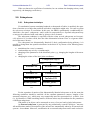
2.8.1.
Subsystem technique.......................................................................................... 2-70
2.8.2.
Standard subsystems .......................................................................................... 2-71
2.8.2.1. Wheelset as standard subsystem ..................................................................... 2-71
2.8.2.2. Vehicle suspensions ....................................................................................... 2-71
2.8.2.3. Caterpillar ...................................................................................................... 2-72
2.8.2.4. Ballast............................................................................................................ 2-72
2.8.3.
Examples of compound objects .......................................................................... 2-72
2.8.3.1. Dynamically independent subsystems ............................................................ 2-72
2.8.3.2. Dynamic platform as a compound object........................................................ 2-73
2.8.3.3. Locomotive as a compound object ................................................................. 2-74
2.8.3.4. Multibody physical pendulum ........................................................................ 2-75
2.9.
Linearization of equations and equilibrium positions............................................ 2-76
2.9.1.
Equilibrium equations and their solving ............................................................. 2-76
2.9.2.
Natural frequencies, modes, eigenvalues and eigenvectors ................................. 2-76
2.10.
Units of measure ...................................................................................................... 2-76
2.11.
Generation and analysis of equations of motion .................................................... 2-77
2.12.
The innovative capacity of the program and programming in its environment ... 2-77
References ........................................................................................................................... 2-77
Universal Mechanism 5.0
2-3
Part 2. Mechanical system
2. Mechanical system as an object for modeling
In this part common definitions necessary for a successful operating with UM are given.
More detailed and complicated information about the object – a mechanical system and the mathematical technique applied to analyze it – the reader can find in the scientific introduction.
2.1. Modeling mechanical systems
Consider a physical pendulum i.e. a rigid body, which has a horizontal rotational axis not
passing through its center of mass. It is a simple example of a mechanical system. Anybody
could imagine the motion of the pendulum and suppose that the pendulum would swing if initially it were not in equilibrium. However, far not everyone can write down ‘off-hand’ the equation
of motion and solve it. Anyway, even junior students of university natural faculties can do it. If
the air resistance force is to be taken into account, the analysis can only be carried out by senior
students. Moreover, if we attach a second body to the first one, even a professional mathematician cannot obtain the exact analytical solution (because it does not exist!). What then can be
said about systems containing dozens, hundreds, and thousands of bodies?
In such cases, applying the following numerical methods for modeling is most effective:
· automatic generation of equations of motion;
· numerical analysis of equations of motion;
· treatment of the results of the equations analysis and their representation in a convenient
form.
There are a lot of concepts for the equations analysis. So choosing one or another is, by
far, determined by the nature of the analyzed system. This might be the numerical integration of
the equations of an object in a complex spatial motion (e.g., for a robot manipulator). For a multibody system (MBS) whose bodies move slightly about a fixed in space position the determination of the natural frequencies and modes is often necessary. A considerable amount of information one could obtain through solving the problem of motion stability in the neighborhood of the
equilibrium position or a steady motion.
The representation of the equation analysis results is most convenient when using computer graphics. So it is possible to simulate motion and to display time-varying charts.
In the course of the system analysis, the designer often has to change its configuration
and parameters (for example, the sizes of the bodies or any coefficients in the expressions for
forces). These changes must be organized by the software as simply as possible. Once the configuration is changed, the equations of motion usually change as well. If the two-body physical
pendulum is to be transformed into a three-body one, the equations will change totally. Here it
matters how fast the equations are generated. The operational changing of parameters of an MBS
is possible without generating the equations anew if they are derived in a fully symbolic form
and the corresponding parameters take part in them as identifiers (data parameterizing).
The program package UM has been designed for solving such and many other problems.
Universal Mechanism 5.0
2-4
Part 2. Mechanical system
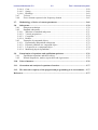
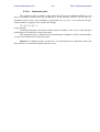
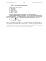
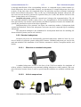
2.2. Rigid body systems
Belt conveyor
Double wishbone suspension of a vehicle (left); truck suspension with hydraulic actuators (right)
Mooring platform and its anchor system
Universal Mechanism 5.0
2-5
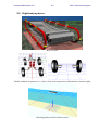
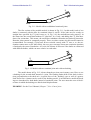
Expander
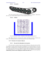
Caterpillar transporter
Щебеночный
балласт
как система
Ballast as
a multibody
system тел
Part 2. Mechanical system
Universal Mechanism 5.0
2-6
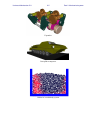
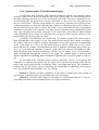
Freight railway vehicles
Electric locomotive EP200
Train model
Part 2. Mechanical system
Universal Mechanism 5.0
2-7
Part 2. Mechanical system
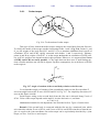
Coach
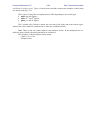
Fig.2.1. Multibody systems
The objects to be dealt with by UM can only be rigid body systems. The bodies of a system may or may not be connected with each other by joints and force elements. In particular, bodies may be mass points (Fig.2.1).
The motion of an MBS is studied with respect to the basic body, by which an inertial system of coordinates (SC) is meant. Often such a system can with enough accuracy be identified
with the surface of the Earth. The basic body is considered fixed and therefore is not included in
the analyzed MBS, although takes an active part in the description of the system. The basic SC is
denoted SC0. Usually, dividing a compound object into bodies is no problem. For example, a
two-body physical pendulum consists of two bodies, whereas the Puma manipulator - of four.
Sometimes, a deformable body, e.g., an elastic beam, can be represented as an MBS. For this representation to be valid the beam has to be divided into several rigid bodies. The separate bodies
are connected with each other by massless elastic elements.
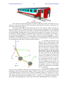
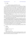
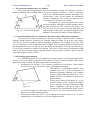
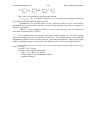
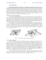
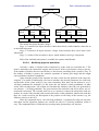
To describe the motion of an
z0
MBS in terms of mathematics the right
Cartesian system of coordinates is associated with each body. Its origin is
z1
placed in any point of the body and the
axes are fixed to it. Generally speaking, the orientation of the axes of the
O
body-fixed SC may be chosen arbitray0
rily, but the equations of motion will
be easier if the axes are the principal
axes of inertia. Here and below such
y1
systems of coordinates are referred to
z2
y2 as the body-fixed systems of coordiO1
x0
nates and denote them as SC [the index of the body], e.g., SC1 is the system of coordinates fixed to body 1. In
a particular case, when a body has axes
x1
O2
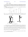
of symmetry, the axes of the bodyFig.2.2
fixed SC are usually directed along the
x2
axes of symmetry.
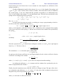
For example, consider a model
of the two-body pendulum, which has two homogenous rods connected by a rotational joint and
attached by a joint to the immovable support. The axes of the joints are parallel and the motion
of the MBS therefore is 2D, however in UM all coordinate systems are assumed to be threedimensional. The basic SC0 Ox0y0z0 has the origin in О, which coincides with the center of the
joint. The body-fixed systems of coordinate O1 x1 y1z1 and O2 x2 y 2 z 2 originate in the centers of
mass of the corresponding bodies, whereas the axes are directed along their axes of symmetry.
Universal Mechanism 5.0
2-8
Part 2. Mechanical system
2.3. Joints
2.3.1. Connectivity of systems and definition of a joint
It is assumed that the modeled MBS satisfies a connectivity condition, i.e. each body of
the system is connected by a joint at least with one other body or the basic body (SC0), and there
exists a path from each body to SC0. This condition is very important and is automatically
checked by UM. By what joint and with what body is an unrestrained body moving in space
connected? And does it make sense at all to introduce joints for free bodies? It appears to be
clear that to describe the position of a body in space it is sufficient to know the position of the
body-fixed SC relative to the basic SC0. In terms of mathematics, for that it is sufficient to set
the position of the origin and the orientation of the body-fixed SC with respect to the basic SC0,
expressing them through certain variables called coordinates. For this purpose, UM uses the dependencies between, on the one hand, coordinates and, on the other, the radius vector of the
body-fixed SC origin and the directional cosine matrix (the matrix of rotation). The term ‘joint’
is intended to describe the position of one body relative to another. To say ‘describe the position
of a body relative to the basic SC0 in terms of coordinates’ means in UM ‘introduce a joint between the given body and the basic one’.
Joints making it possible to describe the position of one body relative to another by
means of introducing the joint coordinates are below denoted as generalized¸ rotational, translational, quaternion and 6 d.o.f. joints. UM uses another type of joints constraining the relative
motion of bodies and which have certain problems in introducing the joint coordinates. In many
systems the constraint represented by a massless rigid rod with joints at the ends is not a generalized joint either although it is also available with UM.
Certainly, generalized, quaternion and 6 d.o.f. joints can be introduced for any pair of bodies both kinematically connected and not. If any two bodies are connected by a joint in the
usual sense - e.g., rotational or prismatic - its representation in UM assumes that the position of
one body will be described relative to the other, namely the position of one body-fixed SC will
be described relative to the other body-fixed SC. The joint coordinates, i.e. the variables setting
this position, are introduced. The complete set of coordinates for the object as a whole is the result of unification of the local joint coordinates. Such a description takes place in the data input
programs and is greatly automated. However, joints to connect each body with the basic one may
not exist, although it is sufficient that there exists for each body a chain of bodies from this one
to the basic. It is the urgent condition of connectivity of the modeled MBS
According to the condition of connectivity, it is also required that joints in the chain be
not arbitrary but of certain types. Currently the following generalized types of joints are available:
· rotational;
· translation;
· six d.o.f. joint;
· generalized;
· internal body joint, based on 6 d.o.g.
· quaternion;
· massless rigid rod constraint;
· mates;
· convel (constant velocity) joint.
Rotational, translation, six degree of freedom and generalized joint belong to a certain
group. They have identical internal representation and describe kinematical pairs with various
translation and rotational d.o.f. (from zero to six). Rotational, translation and six degree of freedom joint can be described with the help of generalized joint.
Universal Mechanism 5.0
2-9
Part 2. Mechanical system
Quaternion joint is often used for introduction of coordinates for a free body and for description spherical joint.
Massless rod, mates and convel joint do not introduce new coordinates. They are just kinematical constraints.
Joints of types
1. rotational;
2. translational;
3. 6 degrees of freedom
have internal UM representation as generalized joints. Conversion of joints to generalized type is
available in the UM Input. This tool can be used to create additional degrees of freedom, to describe joint forces, to parameterize inclination of axis and so on. See Chapt. 3 of user’s manual
for additional information.
Example. User’s manual, Chapt. 7, Sect. Joint type conversion. Parameterization of axis inclination.
Universal Mechanism 5.0
2-10
Part 2. Mechanical system
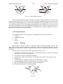
2.3.2. Description of joints
2.3.2.1.
Translational and rotational joints
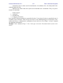
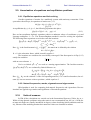
Fig.2.3. Joint with 1 d.o.f.
Translational and rotational joints allows describing one d.o.f. joints. Every joint of this
type introduces one local coordinate (linear or angular). A sketch of such joints is given in
Fig.2.3. There are following parameters:
· joint vector e, described by its projections on SC1 and SC2 (e1x , e1y , e1z ), (e x2 , e 2y , e z2 ) . Vector
cannot be zero.
· coordinates of two joint points (connected with body 1 and body 2) situated on joint axis
(r11x , r11y r11z ), (r 22x , r 22y r 22z ).
·
Some additional parameters, shift along the joint axis xa and/or turning around the joint
axis j a .
Vector (e1x , e1y , e1z ) and point A (r 11x , r11y r11z ) describe the joint axis position relative body
1, and vector (e x2 , e 2y , e z2 ) and point B (r 22x , r 22y r 22z ) describe the joint axis position relative body 2.
If xa = 0 then points A and B are coincide (have the same coordinate in SC0).
The xa parameter in the case of a translational joint and the j a parameter in the case of
a rotational joint are used for describing the relative positions of the bodies when the coordinate
is zero.
Positive rotation corresponds to the right-hand screw rule.
There might be introduced joint force in a translational joint and joint torque in a rotational joint.
Local coordinates for both joint types might be described as explicit time functions. In
that case joint coordinates is not included to the list of coordinates of object. For example, angle
of rotation might be describes as j(t ) = wt , where w is the angular velocity.
Universal Mechanism 5.0
2-11
Part 2. Mechanical system
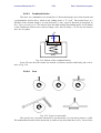
Examples
Fig.2.4. Rotational and translational joints
Here the rotational joint (Fig.2.4 left) is described by the following parameters:
e1x , e1y , e1z = (1,0,0), e x2 , e 2y , e 2z = (1,0,0),
(
)
(
)
(r11x , r11 yr11z ) = (0, a,0), (r22 x , r22 yr22 z ) = (0,-b,0) ,
xa = ja = 0 ,
And here the translational joint (Fig.2.4 right) is described by the following parameters:
e1x , e1y , e1z = (1,0,0), e x2 , e 2y , e 2z = (1,0,0),
(
)
(
)
(r11x ,r11 yr11z ) = (r22 x ,r22 yr22 z ) = (0,0,0) ,
xa = ja = 0 .
Universal Mechanism 5.0
2.3.2.2.
2-12
Part 2. Mechanical system
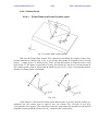
Six d.o.f. joint
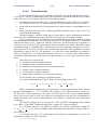
Joints of such a type are often used to introduce kinematical pairs with various numbers
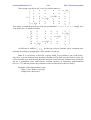
of rotational and translation d.o.f. Consider two bodies: 1 and 2 (see Fig.2.5). Origins of bodyfixed SC are located in points O1 and O2. Introduce two additional SC: SC1A and SC2B with its
origins in some points A and B correspondently. The joint introduces coordinates, which describe the position of SC2B relative to SC1A.
O1
r1
B
r2
A
O1
Fig.2.5
By default the joint has six d.o.f.: three shifts SC2B relative to SC1A (x, y, z) and three angles of SC2B orientation relative to SC1A ( a1, a2 , a3 ). In this case body 2 moves freely and joint
does not introduce any constraints on relative movement.
There are 12 ways of introduction of orientation angles accordingly sequence of rotations
around axes (x-1, y-2, z-3):
· Euler (3,1,3);
· (3,2,3);
· (2,1,2);
· (2,3,2);
· (1,2,1);
· (1,3,1);
· Cardan (1,2,3);
· (1,3,2);
· (2,1,3);
· (2,3,1);
· (3,1,2);
· (3,2,1).
Any of these six d.o.f. might be turned off. It means that the d.o.f. will not be introduced
in a model. A lot of various kinematical pairs might be described in that way.
The following parameters are necessary for description the six d.o.f. joint:
- coordinates of points A in SC1 and B in SC2 r11x , r11 y r11z , r 22 x , r 22 y r 22 z as well as
orientation of SC1A and SC2B relative to SC1 and SC2;
- type of angle orientation;
- enabled/disabled d.o.f.
(
·
)(
)
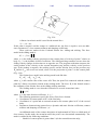
Consider some examples.
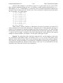
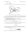
Spherical joint (see Fig.2.56). Vectors r1,r2 describe the position of the center of the
joint in SC1 and SC2, all translation d.o.f. are disabled. Here the spherical joint (Fig.2.6)
Universal Mechanism 5.0
2-13
Part 2. Mechanical system
is described by the following parameters: r1 = 0 , r2 = (0,0,-a ) , type of orientation angles is (3,1,3).
Fig.2.6. Spherical joint
Fig.2.7. Hooke (universal) joint
·
Hook joint with two d.o.f. (see Fig. 2.7). All translations and one of rotational coordinate
are disabled. Vectors r1,r2 describe the position of the center of the joint in SC1 and
SC2. For the joint in fig. 2.7: r1 = (0, a,0) , r2 = (0,-b,0) , type of orientation angles is
(1,2,3), the angle a2 is turned off (or the type is (1,3,2) and a3 is turned off).
·
One d.o.f. joints. Let us consider examples in Fig.2.4. For a rotational joint we have
(r11x ,r11 yr11z ) = (0, a,0), (r22 x , r22 yr22 z ) = (0,-b,0) ,
all translations are disabled and two rotational ones, too. For example, these are angles
a2 ,a3 for the orientation angles of type (1,2,3). For a translational joint r1 = r 2 = 0 , all the
angles are disabled and translations x, z, too.
Remark. It is well known, that there are singular orientations of SC2 relative to SC1 for
any type of three orientation angles. In the singular orientations, the numerical values of the
orientation angles cannot be found uniquely, which results in failure of the simulation of motion.
The first six types (axes of the first and the last rotations have the same indices) are singular at
a2 = 0, p . The rest six types have singularities when a2 = ± p 2 . This fact must be taken into
account for spherical joints, if SC2 can have an arbitrary orientation in respect to SC1 while simulation of motion. For example, do not use orientation angles being singular at a2 = 0, p , if axes
of SC2 are parallel to those of SC1 at begin of simulation (when t=0). Generally, in case when a
free body can have an arbitrary spatial orientation at run-time, use the quaternion joint instead of
six d.o.f. one.
Universal Mechanism 5.0
2.3.2.3.
2-14
Part 2. Mechanical system
Generalized joint
Most of kinematical pair can be modeled with the help of joints described above. However, there are a variety of kinematical pairs, which cannot be described with the help of those
joints. Here is a list of examples, which is far from being complete:
· a Cardan joint, whose rotation axes are not perpendicular; or whose first axis is not parallel to some of axes of SC1; or whose second axis is not parallel to some of axes of SC2;
· joints with more than one d.o.f. having joint forces and/or torques, corresponding some of
d.o.f.;
· joints with more than one d.o.f. realizing predefined motion (some or all of d.o.f. are
time-dependent functions).
All these examples, and also all the types of joints above, can be implemented using the
generalized joint. Mathematical model of the joint is discussed in the scientific manual.
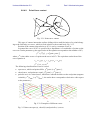
So, the generalized joint, by definition, is a constraint having an arbitrary number of both
translational and rotational degrees of freedom (from 0 to 6). The transition from SC1, connected
with the first body, to SC2, connected with the second one, can be described as a sequence of
elementary transformations (ET) at an arbitrary relative position of the bodies. Each ET is either
a translation along or a rotation about a certain direction. Let us introduce concepts of a vector e
and a parameter s of an ET. The unit vector e defines the direction of the translation or rotation
(depending on type of the ET). The parameter s (i.e. the value of the translation or rotation) is
either a constant value or a certain time-dependent function, or a variable value, which must be
calculated at simulation time. In the latter case, the parameter s is a local generalized joint coordinate.
Thus, there are six types of ET:
· tc - translation with a constant parameter;
· tv - translation with a variable parameter;
· tt - translation whose parameter is a known time function;
· rc - rotation with a constant parameter;
· rv - rotation with a variable parameter;
· rt - rotation whose parameter is a known time function.
Let us consider some examples of generalized joints.
a) A rotational kinematic pair (Fig. 2.4 left). It is described by three ETs:
T1 = {tc, e y , a}, T2 = {rv, e x ,j }, T3 = {tc, e y , b}, q ij = [j ] .
Before starting the explanation of the expressions, it seems appropriate to make clear the
introduced designations. T1, T2, T3 stand for the consecutive ETs. Then in brackets, the type of
ET, the vector e and the parameter s are given. For all the types of ETs, except constant translation tc, the vector e must be unit. For tc there are no parameters since the value of translation is
directly included in the vector of transformation. The column qij contains the list of local joint
coordinates.
The first ET translates SC1 by a along axis y. The second ET corresponds to the rotation
by j about x. The final ET (transition along axis y) makes SC1 coincide with SC2.
b) A prismatic joint (Fig. 2.4 right) in a simplest case can be described by a single ET
T1 = tv, e y , s , q ij = [s ] ; s is the coordinate which determines the translation of body 2 with re-
{
}
spect to body 1.
c) A Cardan joint (Fig. 2.7) is a kinematical pair having two rotational d.o.f. In the case
sketched in the figure it is set by four ETs:
T 1 = {tc , e = ( 0 , a ,0 ) } ,
Universal Mechanism 5.0
2-15
Part 2. Mechanical system
T 2 = {rv, e = (1,0 ,0 ), s = a 1 } ,
T 3 = {rv, e = (0 ,0 ,1), s = a 2 } ,
T 4 = {tc, e = (0 , b,0 )} ,
q = [a 1 , a 2 ] .
T
ij
T1 translates SC1 by a along the axis y and the axis x occupies the position of the first axis
of rotation. The second ET (the rotation by a1 about x) brings the axis z into coincidence with the
axis of the second rotation. These are followed by the rotation by a2, which makes the axes of
the SC parallel to those of SC2. The final ET - the translation along y - results in the coincidence
with SC2.
Notice that every next ET is done relative to the new position of SC, in which the preceding ETs resulted. As a rule, ETs cannot be exchanged, thus, in other words, ETs are not commutative.
a)
b)
Fig.2.8. Two joints with the same set of ETs but with different their sequence
E.g., if, in the case of the Cardan joint shown in Fig.2.7, one exchanges the second and
third ETs, it will result in a Cardan joint with a totally different kinematic structure (Fig.2.8a). If
one exchanges the first and second ETs, the resulting pair will not be a Cardan joint at all but a
joint with two d.o.f. (Fig.2.8b). This pair is also available with UM, although it by no means corresponds to Fig.1.3с. These examples show that the concept of common joint is far not trivial
and while describing it there may appear serious and hardly detectable errors.
d) A spherical joint. Bodies connected by spherical joints may have arbitrary relative
orientation. In the example of a Lagrange top shown in Fig.2.6 (a symmetrical body connected
with the support by a spherical joint whose center lies on the axis of symmetry), the transfer
from SCI to SCJ is carried out in two stages. First, rotate SCI so that its orientation coincide with
SCJ and then make a translation along the axis z. Bringing the two systems of coordinates into
coincidence might be obtained by rotating about three axes. So three angles of orientation are
introduced. To introduce the three angles one can use any of the twelve allowable combinations
of the axes of rotation. However, in the case of a Lagrange top Euler angles are conventional.
Thus, here the spherical joint is described by the following four ETs:
T1 = {rv, e = (0,0,1), s = y } ,
T2 = {rv, e = (1,0,0), s = J} ,
T3 = {rv, e = (0,0,1), s = j},
T4 = {tc, e = (0,0, a )},
qij = [ y , J, j]T .
Universal Mechanism 5.0
2-16
Part 2. Mechanical system
And the final example is a free body in space. It is a joint with six d.o.f. and six ETs:
three variable translations along the axes x,y,z and three variable rotations about the axes z,x,z Euler angles, or x,y,z - Cardan angles, or, at last, any series of rotations about three arbitrary axes
(one has to bear in mind, however, that the axes of two consecutive rotations must not be parallel). For instance, for Cardan angles:
T1 = {tv , e = (1,0,0), s = x},
T2 = {tv , e = (0,1,0), s = y},
T3 = {tv , e = (0,0,1), s = z},
T4 = {rv , e = (1,0,0), s = a },
T5 = {rv , e = (0,1,0), s = b },
T6 = {rv , e = (0,0,1), s = g },
q ij = [ x , y , z, a , b , g ] T .
When solving various problems of kinematics and inverse problems of control ETs
whose parameters are explicit time functions are frequently used. It means that how the angle of
rotation or the parameter of translation changes with time is known a priori. E.g., while solving
the kinematic problem of the crank-and-slide mechanism the motion of the input link - the crank
- is given. Here the angle of rotation in the joint connecting the crank with the fixed support
changes in a known manner, for example, it can be linear with respect to time.
Remark. The generalized joint with three rotational d.o.f. can be singular at some relative orientations of the bodies in pair (see remark in Sect. 2.3.2.2). In case if the bodies can be
arbitrary oriented while moving, values of the orientation angles may become (almost) singular.
This results in a strong deceleration or a total break of simulation of motion due to automatic decreasing the integration step. Because of this reason, in this case it is recommended to use the
quaternion joint, which does not have any singularities.
Universal Mechanism 5.0
2.3.2.4.
2-17
Part 2. Mechanical system
Quaternion joint
The quaternion joint is similar to that with 6 d.o.f. The most significant difference consists in coordinates, which define the orientation of SC2B relatively to SC1A. In the case of a
quaternion joint we have four coordinates (a quaternion) q0 , q1, q2 , q3 . As it is known, the quaternion cannot be singular, but it satisfies the identity
q02 + q12 + q22 + q32 = 1
at any moment.
Translational degrees of freedom can be turned off similar to the 6 d.o.f. joint, but rotational degrees of freedom are always presented.
The quaternion joint is mainly used for introducing coordinates of freely moved bodies,
as well as for introduction of spherical joints.
Remark. If a spherical joint is cut (Sect.2.3.3), its description by a quaternion joint is the
most effective way from the numerical point of view.
Universal Mechanism 5.0
2.3.2.5.
2-18
Part 2. Mechanical system
Internal body joint
Internal body joint is often used by introducing 6 degrees of freedom to a body, which
can move freely. Orientation angles in these case correspond to the sequence of rotations 1,2,3
(Cardan angle).
A large weight is automatically assigned to the internal body be the program. Due to this
fact, if a joint or a chain of joints setting position of the given body relative to the Base0 is introduced, the internal joint is cut and automatically removed. This property of internal joints is frequently used in subsystems in particularly in specialized UM modules such as UM Caterpillar
and UM Train3D.
Consider an example. In the UM Caterpillar module the model of a track is automatically
generated as an included subsystem. All elements in the subsystem, which must be connected
with the hull, are connected with a fictitious body. The fictitious body has six d.o.f. introduced
by an internal joint. In the model of a tracked vehicle, the model includes a hull with 6 d.o.f. and
two subsystems – tracks. Fictitious bodies from each of the subsystems are rigidly fixed relative
to the hull by special zero d.o.f. joints. In this case the internal joints of fictitious bodies are cut
and automatically removed.
Universal Mechanism 5.0
2.3.2.6.
2-19
Part 2. Mechanical system
Weightless rod constraint
This type of constraint corresponds to a weightless rod with spherical joints at the end
points connecting two bodies. There is no friction in the joints. To describe the constraint it is
enough to set the coordinates of the attachment points of the rod in the body-fixed SC of both
bodies and a nonzero length of the rod. The length of the rod may be either constant or an explicit time function, which greatly expands the area of its application to analyze controlled systems.
E.g., an actuator may be considered a massless rod with the length varying somehow in a number
of problems where its inertial parameters are insignificant.
Universal Mechanism 5.0
2.3.2.7.
2-20
Part 2. Mechanical system
Mates
Mates are constraints, which limit relative position and motion of pairs of bodies. The notion ‘mate’ is introduced in CAD programs and appears in UM in connection with development
in UM40 interfaces to CAD programs such as SolidWorks, Autodesk Inventor, KOMPAS. As a
rule, mates appear in UM models as a result of converting CAD assemblies into UM objects
when some constraint cannot be converted automatically in joints described above.
Mates realized in UM a described by the following data.
1. Type of mate
· Coincident
· Concentric
· Parallel
· Distance
· Angle
2. Type and parameters of manifolds connected with each of the in the pair of bodies
· Point. Described by coordinates in the body-fixed SC.
· Line. Described by coordinates of one point on the line and a unit vector along it in the
body-fixed SC.
· Plane. Described by coordinates of one point on the plane and a normal to the plane in
the body-fixed SC.
3. Parameters, which depend on the mate type.
· Distance. Distance between the manifolds should be specified.
· Angle. Value of angle between the manifold must be set.
There exist limitations on type of manifolds for some types of mates. For instance, manifolds
cannot be points for mates “coincident”, “parallel” и “angle”.
Example. Mate of the “coincident” type with points as manifolds for both of the bodies, i.e.
the coincidence of a point of the first body with another point of the second body, introduces the
same constraints on relative motion of the bodies like a spherical joint. The main difference consists in the fact that if the spherical joint is not cut, it introduced 3 angular degree of freedom defining orientation of the second body relative to the first one. The mate always adds constraint
equations, 3 equations in the considered case:
r1 + A01r11 - r2 - A02 r 22 = 0
Here r1, r2 are the radius-vectors of body-fixed system of coordinates, A01, A02 are the direct
cosine matrices of body-fixed SC, r11, r 22 are the radius-vectors of coinciding points, which are
specified in the body-fixed SC.
Universal Mechanism 5.0
2-21
Part 2. Mechanical system
Number of constrain equations for all possible types of mates is specified in the table.
Type of mate
Types of manifolds
Coincident
point-point
point-line
point-plane
line-line
line-plane
plane-plane
line-line
line-line
line-plane
plane-plane
point-point
point-line
line-line
line-plane
plane-plane
line-lineя
line-plane
plane-plane
Concentric
Parallel
Distance
Angle
Number of constraint
equations
3
2
1
4
2
3
4
2
1
2
1
1
3
2
3
1
1
1
Universal Mechanism 5.0
2.3.2.8.
2-22
Part 2. Mechanical system
Convel joint
O2
e2
O1
e1
A
Fig. 2.9. Scheme of ConVel joint
A ConVel (constant velocity, CV) joint provide equal angular velocities of a pair of inclined shafts. This constraint corresponds to a point-point coincidence mate as well as to equal
shaft angles of rotation.
The joint is specified by the coordinates of the joint center A in SC of each of the bodies
as well as by two unit vectors e1, e2 for shaft axes, Fig. 2.9.
The joint adds four constraint equations. Three of them correspond to coincidence of two
points A of shafts. The fourth equation provides the equality except for sign of angle of rotation
of body 2 about vector e2 and the angle of rotation of body 1 about the vector e1.
Remark. In fact, the joint does not provide constant angular velocities of shafts. The name of the
joint reflects its property to keep (nearly) constant velocity of the second shaft by the constant
angular velocity of the first one, unlike the Hook joint. Besides, angular velocities of shafts are
(nearly) equal.
To make the CV joint model correctly, the user should create a correct kinematic scheme
of shafts by proper choice of joints and/or force elements.
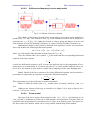
S
Fig. 2.10. Model configuration with additional rotational joint
At the beginning consider a model, which does not correct with respect to the CV joint.
In this model the first shaft is connected with the base by a rotation joint S, Fig. 2.10, and 6 d.o.f.
are introduced for the second shaft relative to SC0. In this model a CV joint reduces the degrees
of freedom of the second shaft to two rotational d.o.f. relative to shaft 1. In such the model, the
second shaft does not keep it orientation along the axis e2, and the shaft motion is not correct.
Universal Mechanism 5.0
2-23
Part 2. Mechanical system
S2
S1
Fig. 2.11. Model with two additional rotational joints
The first variant of the possible models is shown in Fig. 2.11. In this model each of two
shafts is connected with the base by rotational joints S1 and S2. If the joint axes lie exactly on
straight lines specified by CV joint vectors e1, e2, Fig. 2.10, the mechanism works properly. At
the same time, the second shaft without CV joint has 1 d.o.f. only, and adding the CV joint introduces four constraints. This means, the model has redundant constraint and statically uncertain.
Reaction joints cannot be computed properly. There are other reasons why this model cannot be
recommended. For example, if joint axes do not coincide exactly with CV axes e1, e2, the mechanism cannot move at all. Most likely, the user gets a message about non-consistent equations
of motion by the start of simulation. As a rule, this scheme is incorrect if the shafts are connected
with different bodies, which can move relative to each other.
S1
Fig. 2.12. Model with one rotational joint and with one bushing
The model shown in Fig. 2.12 is better than the previous one in many cases. Here we see
a bushing for the second shaft instead of a joint. The bushing limits shifts of the body in directions perpendicular to the shaft axis. A special force of the ‘bushing’ type as well as a generalized linear force element can be used for the bushing model. In an alternative model the bushings are introduced for both shafts instead of rotational joints. The user must take care of the directions in which the bushings are blocks shaft displacements.
EXAMPLE. See the User’s Manual, Chapter 7, Sect. Convel joint.
Universal Mechanism 5.0
2-24
Part 2. Mechanical system
2.3.3. System graph. Closed kinematical loops
An important stage in dealing with complex mechanical systems is the analysis of their
structure, which can be carried out with the help of the system graph. Its vertices correspond to
the bodies including the basic one; its ribs correspond to the joints. The above conditions of connectivity being met, the graph of the system is connected, i.e. there is at least one path between
any two of its vertices. That the graph satisfies the connectivity condition is the corollary of the
condition that there is a chain for each body that connects it with body 0 (base, SC0). If there is
but one path between any pair of vertices, the graph is a tree, and in this case the corresponding
mechanical system has a tree structure. If at least one pair of bodies between which there exists
more than one path can be found, the graph of the system has cycles and the MBS contains
closed kinematical loops. Then it is clear that there are bodies in the systems, which are connected with body 0 by more than one chain.
A majority of mechanisms has closed loops. To analyze systems with closed loops is
more difficult than if the system is a tree. The most effective strategy here consists in cutting a
few joints so that a tree could be obtained. The number of cut joints equals that of independent
cycles in the graph. It is easy to see that almost always to choose which joints to cut is ambiguous and there is a chance of picking them out best or optimally considering this or that criterion, e.g., to facilitate the equations of motion, reduce their size, decrease the number of arithmetic operations in the numerical modeling of motion, etc. In UM the choice of such joints is
made automatically through the analysis of the graph. The optimal cutting is based on the
Dijkstra algorithm for obtaining paths of minimal weight from the root of the graph to each vertex.
As was noted in the section devoted to system connectivity (Sect.1.3.1), to generate the
equations in a symbolic form requires that the joints in the chain between the basic body and any
body of the system must introduce coordinates. Thus, a rod joints must be cut. The condition of
connectivity, for this reason, requires sometimes the introduction of additional joints with six
d.o.f. for a spatial problem and three d.o.f. for a 2D one.
Remark 1. The user can have an influence on the choice of joints to be cut by means of
large weight coefficient for the corresponding joint in the closed loop.
Remark 2. Cut joints with 6 degrees of freedom are conditionally removed, i.e. the corresponding coordinates are not included in the set of object coordinates.
Universal Mechanism 5.0
2-25
Part 2. Mechanical system
2.4. Equations of motion
Equations of motion of a multibody system have the following form of differentialalgebraic equations:
(2.1)
M (q, t )q&& + k (q, q&, t ) = Q (q, q& , t ) + G T (q )l ,
h (q, p ) = 0,
where q is the column of basic coordinates of the system, p is the column of auxiliary coordinates (local joint coordinates in cut joints; M is the mass matrix, k,Q columns of generalized inertia and applied forces; l are Lagrange multipliers corresponding to reactions in cut joints; the
second equation in Eq. (2.1) is the algebraic constraint equation corresponding closure conditions of cut joints. Matrix G is the Jacobian matrix of the constraint equations after elimination of
auxiliary coordinates.
UM generates the equations of motion in a symbolic form. This approach proved to be
more efficient in comparison with a purely numerical one.
Consider expressions generated by UM for each simple object. Let q = qij be the set of
{ }
coordinates of the object. It contains the local joint co-ordinates for normal and fictitious joints
(except the cut normal joints. UM generates in a symbolic form the following kinematic relations:
· The radius-vectors of mass centers and rotation matrices for each body,
ri0 = ri0 ( q, t ), Ai 0 = Ai 0 ( q, t ),
· The velocities of mass centers and angular velocities for each body,
vi0 = Di0 q& + v '0i ,
wii = Bii q& + w'ii ,
· Note that all quantities relating to body rotations are given in the body-fixed SC, whereas
all translational quantities are set in the SC0;
· The matrices Di0 and Bii included in the expressions for the velocity of the center mass
and angular velocities (Jacobean matrices);
· The vectors a 'i0 and e' ii of the terms of accelerations and angular accelerations not depending on q&& ,
·
·
ai0 = Di0 q&& + a 'i0 , eii = Bii q&& + e'ii ;
Constraint equations for the cut joints
hk (q, pk ) = 0 .
Elements of the matrices M , k , Q of the motion equations (2.1)
Universal Mechanism 5.0
2-26
Part 2. Mechanical system
2.5. Theoretical foundations for solving constraint equations
Theory of numerical solving differential-algebraic equations asserts that the numeric
solvers are sensitive to errors in initial conditions. This means that the initial values of coordinates and their first time derivative should satisfy the constraint equations as exactly as it is possible. To clarify the problem it is good to consider the procedure of forming and solving the constraint equations.
Let q0 , p0 be the current values of generalized (coordinates in joints, which belongs to
the object tree, i.e. they are not cut) and auxiliary coordinates, respectively. These values, as a
rule, do not satisfy the constraint equation
h(q,p)=0,
which corresponds to the closure conditions for the cut joints. The corrections Dq, Dp must be set
so that new coordinate values satisfies the equation
(2.2)
h(q0+Dq, p0+Dp)=0.
The Newton-Raphson iterations are used by UM for solving the nonlinear Eq.(2.2). The following equations are solved at every the iteration:
Hq(qk, pk)Dqk+1 + Hp(qk, pk)Dpk+1 = -h(qk, pk),
qk+1= qk + Dqk+1, pk+1= pk + Dpk+1, k=0,1...
q0= q0 , p0= p0.
Here Hq, Hp are the Jacobian matrices of the vector h. The k-th iteration is done according to the
following pattern. The constraint equations
(2.3)
Hq,i(qk, pki)Dqk+1 + Hp,i(qk, pki)Dpk+1i = -h(qk, pki),
are generated for each cut joint j. This equation is in the generalized coordinates and local auxiliary variables (i.e. the local coordinates in the cut joint). The auxiliary variables Dpk+1i are eliminated from Eq.(2.3) with the help of the Gauss elimination procedure and the following two equations are obtained:
(2.4)
Dpk+1i = PiDqk+1 +d pki ,
k
k+1
k
(2.5)
Gi Dq = -gi .
Then Eqs. (2.5) for separate cut joints are added to the matrix equation
(2.6)
GkDqk+1 = -gk,
whose solution are obtained using the Gauss elimination procedure based on the row pivoting.
The correction values for the pivotal elements (independent variables) are set to zero and nonzero values of the dependent variables are calculated according to Eq.(2.6). The obtained solution
Dqk+1 is substituted into Eqs.(2.4) for evaluations of the auxiliary variables. If the norm of the
calculated correction vector is less that the prescribed small tolerance e, the iteration is stopped
and the program exits from the procedure otherwise the next iteration is executed.
Note that according to this algorithm, an arbitrary solution to the equations is obtained in
agreement with the constraint equations. Fixing coordinates (e.g., when it is necessary to obtain
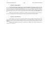
the configuration of a four bar mechanism for a certain angle of crank rotation, Fig. 2.13), can be
done by the user but only for generalized coordinates (not auxiliary!). The fixed coordinate remains unchanged during the above iterations.
The process of automatically solving the constraint equations can fail. If it does not converge after 20 iterations, you receive the corresponding message and can either continue the
process or quit.
Consider some situations when iterations do not converge.
Universal Mechanism 5.0
2-27
Part 2. Mechanical system
·
The constraint equations have no solution
That means the mechanism has not been assembled correctly. For instance, consider a
planar mechanism shown in Fig. 2.13. If one sets the lengths of bodies 1, 2 and 3 so that their
sum is less than the distance between the hinges connecting body 1 and 3 to the support, the mechanism
cannot be assembled. This occurs, too, when the axes
of rotation of the joints are not parallel.
UM cannot see if your mechanism can or cannot be assembled. Although it sends a message notifying that iterations do not converge. Of course, you
have to find out the reason why this happened and
Fig. 2.13. Four bar mechanism
make changes in the object description using the Input
Module or correcting the values of some identifiers.
·
Constraint equations have no solution for the given values of the fixed coordinates.
If you have fixed some coordinates (see previous sections) so that their values cannot be
changed during iterations, sometimes the solution cannot be found. It can be for two reasons.
First, the set of fixed coordinates contains dependent coordinates. For example, if you have fixed
any two coordinates for the mechanism shown in Fig. 2.13, the solution cannot be found because
the mechanism has one d.o.f. and any two coordinates are dependent. Second, if the current value of a fixed coordinate is outside of its interval. This occurs (for the case of mechanism in Fig.
2.13) if you have fixed the angle j1 and the distance between points A and B is greater than the
sum of the lengths of bodies 2 and 3.
·
Bad starting approximation
It is well known that the Newton-Raphson procedure requires a good starting approximation q0, p0 for successfully solving non-linear equations. If your current coordinate values are far
from the desirable solution, the following variants may take place:
à Iterations do not converge. Try to continue iterations for several times. If the solution
is not found jet, try to set the start values of coordinates manually.
à UM obtains an undesirable solution. This
problem arises due to lack of uniqueness of
nonlinear constraint equations. One example
is given in Fig. 2.14 (the dashed line). Use a
manual choice of coordinates to improve the
approximation.
à For the given values of coordinates q0 , p0 the
Jacobian matrix of the constraint equations
(2.6) is singular. For the mechanism in Fig.
Fig. 2.14.
2.14, a singularity of the given kind is encountered if the joint between bodies 1 and 2
is cut and the angles in joints satisfy j3=0,p, j4=j1+j3. Use a manual choice of coordinates to avoid the singular position.
à The Jacobian matrix Hp,i in Eq. (2.4) is singular for the given values of q0 , p0. Use a
manual choice of coordinates to avoid the singular position.
Universal Mechanism 5.0
2-28
Part 2. Mechanical system
2.6. Force elements
Forces acting between bodies are generally divided into applied and constraint reactive
forces. In their turn, reaction forces are represented by two components: the tangential component performing mechanical work during motion (as a rule, these are friction forces) and an ideal
- or normal - component. If all the constraints in the MBS are ideal, the first component is absent. In terms of data input applied forces and the reaction force non-ideal components have the
following in common: they should be expressed through the variables and parameters of the system. However the ideal components of reaction forces are determined by the type of constraint
and their computation is carried out automatically.
In UM the following active forces varying in the patterns of their description in the data
input module, are available:
· gravity forces;
· joint forces (for translation, rotational and generalized joints);
· bipolar forces;
· generalized linear force elements;
· contact forces;
· gearing;
· T-forces;
· externally formulated forces.
An applied force may be a function of time, coordinates and their first time derivatives.
In simpler cases, (e.g., for gravity and generalized linear force element) these functions are automatically generated by the program. However, they are so often quite complicated and the user
has to write his/her own procedures in a control file or use external libraries. Such forces are referred to as externally formulated forces.
Universal Mechanism 5.0
2-29
Part 2. Mechanical system
2.6.1. Gravity
In UM the gravitation field is assumed homogenous. Thus it is only necessary to specify
the unit vector of the gravity direction. The gravity acceleration is assumed 9.81 m/s2. However,
the user can leave gravitation out of account. The generalized forces corresponding to gravity are
generated automatically.
Universal Mechanism 5.0
2-30
Part 2. Mechanical system
2.6.2. Joint forces and torques
One way to set an active force or torque is to introduce these for the corresponding degree of freedom. Thus, one models an engine, actuator (transmission) and other systems where
dynamic effects are insignificant. E.g., in a robot manipulator model the designer has the right
not to take into account inertial properties of the transmission members and therefore not to solve
the dynamic problem. So the model is idealized, and the designer assumes that the influence of
the transmission on the object is reduced to the appearance of driving forces or torques in the kinematic pairs. Such force (torque) is directed along the axis of the pair.
To model such forces in the program the definition of a joint force (torque) for generalized, rotational and translational joints is introduced. In the case of a generalized joint, a force (a
torque) can be introduced for any ET with a variable parameter (i.e. tv or rv, see Sect. 2.3.2.3).
The force (torque) vector is directed along the axis of ET according to the increase of the parameter values. It is assumed that the force is only a function of time, the corresponding ET parameter and its time derivative (that is velocity). This limitation is removed if the user applies the
external description of the force, in other words, if the force computation is done while the modeling of motion with the help of a procedure written by the user in a control file.
For a joint with several d.o.f. it is possible to introduce a force for each d.o.f., or for some
of them.
Universal Mechanism 5.0
2-31
Part 2. Mechanical system
2.6.3. Bipolar forces
Oi
ri
-F
Oj
rj
A
F
B
r
Fig.2.15
A bipolar force element connects two chosen fixed points of a pair of bodies (attachment points
Oi, Oj in
Fig.2.15). The force acts along the straight line between the points and may depend on
time t, the distance r between the points and its time derivative r × ,
F = F (t , r , r . ) .
The force is positive in the repulsion case, for example, it is positive in the case shown in
Fig.2.15.
In the UM input module some of the most often met types of the dependencies between
the bipolar force and the variables are available: a linear function, an analytical expression, a set
of points etc. Mathematical models for this dependence are described in Sect. Types of scalar
forces.
If the distance r equals zero, the degeneration of the force element occurs (due to the uncertainty of the force direction). Here, the force is assumed to be zero.
Example. Consider a bipolar force, which models a linear viscoelastic force element with
c and d parameters as stiffness and damping coefficients. Let the force equals F0 when the length
of the element is x0 and the velocities vanish. The analytic expression for the force looks like
F=F0-c(x-x0)-dv.
Universal Mechanism 5.0
2.6.1.
2-32
Part 2. Mechanical system
Scalar torque
m
O1
r1
B
A
r2
O2
Fig. 2.16. To the notion of scalar torque
This type of force element describes torque acting on the second body from the first one/
To clarify the model of the torque consider interacting bodies 1 and 2, Fig. 2.16. Points O1 and
O2 are the origins of the body-fixed SC1 and SC2. Let us introduce additional local system of
coordinates SCA1 and SCB2, rigidly connected with bodies 1 and 2 respectively. Arbitrary
points A and B are origins of local SC. A scalar torque m depends on orientation of SCB2 relative to SCA1 and does not depend on their origin positions. Moreover, it is supposed that Z axes
of SCB2 and SCB1 are nearly parallel, i.e. the angle between these axes is small during motions of bodies and does not exceed 10 degrees. By these assumptions, let us shift axes of SCB2
to the origin A.
Z1,2
B
X1
α
X2
Fig. 2.17. Angle of rotation of the second body relative to the first one
Let us introduce angle α of rotation of the second body relative to the first one about Z
axis as an angle between the X-axes of SCB2 and SCA1, Fig. 2.17. For simplicity directions of Z
axes on this figure coincide.
Scalar torque acting on the second body from the first one is directed along Z axis of
SCA1. Value of the torque depends on the angle α, its time derivative a& , and time t
m = m (a, a& , t )
Mathematical models for this dependence are described in Sect. Types of scalar forces.
Remark. If the second body is connected with the first one by a rotational joint, which
axis coincides with the Z-axis of SCA1, and Z-axes of SCA1 and SCB2 coincides so that the angle α is equal to the joint coordinate, the scalar torque can be equivalently described by a joint
torque, see Sect. Joint forces and torques.
Universal Mechanism 5.0
2-33
Part 2. Mechanical system
2.6.2. Types of scalar forces
Definition of a bipolar/joint/axle force includes its mathematical model as a scalar function f = f ( x , v, t ) . In the case of a joint force the arguments x,v a the joint coordinate and its
time derivative, for a bipolar force element they are the element length and its time derivative.
Anyway, t is the current time value. The following types of description of the force model are
foreseen in UM.
2.6.2.1.
Linear force
The model corresponds to a linear viscoelastic interaction with a harmonic excitation:
f = F0 - c( x - x0 ) - dv + Q sin(wt + a)
Here F0 is the constant component of the force, c, d are the stiffness and damping constants, x0
is the value of the coordinate x for zero value of the elastic component, Q , w, a are the amplitude, the frequency and the initial phase of the harmonic excitation.
The element is used for description of linear springs, damping elements, harmonic excitations and their combinations
Adding a new element of this type to a model see in Chapt.3, Sect. Input of bipolar force
elements | Linear force element.
2.6.2.2.
Friction force
This type of force is mainly used for modeling frictional dampers. The force description
includes two modes: sliding and sticking. In the sliding mode the force satisfies the formula
f = - Fsign (v )
analogously to the Coulomb friction with a constant friction force F, and v as a the sliding velocity. In the sticking mode, the force model looks like
f = f 0 - c (x - x0 ) - d × v ,
i.e. presents a linear viscoelastic force with the c and d parameters as stiffness and damping coefficients.
The sliding-sticking transition occurs at the moment when the velocity v changes its sign.
At this moment the force f and the coordinate x values are stored (the f0 and x0 parameters in the
formula for the force in the sticking mode).
The sticking-sliding transition occurs when the force reaches its maximal value
f ³ F0 ,
where F0 is the maximal value of static friction force.
The user should specify the parameters of the model F , c, d , F0
Adding a new element of this type to a model see in Chapt.3, Sect. Input of bipolar force
elements | Friction and elastic-friction elements.
2.6.2.3.
Elastic-frictional force
This is one of well-known models of friction, which consists of a dry friction with a linear spring in series. An additional damper is usually set in parallel with the spring (Fig. 2.18).
Universal Mechanism 5.0
2-34
Part 2. Mechanical system
Fig. 2.18
The mathematical model of the element requires the introduction of an auxiliary variable
*
x in addition to x, v variables. In a sliding mode the mathematical model includes the following
differential equations relative to the x * variable:
(2.7)
- d v - x& * - c x - x * = sgn x& * × F
(
) (
)
f = sgn x& * × F .
Here c, d are the stiffness and damping coefficients, F is the constant friction force. The
equation corresponds to a condition that the friction force is equal to the sum of the elastic and
damping forces.
In a sticking the x * variable is constant, and the force is equal to
f = - dv + c x * - x
Stick-slip transition occurs when
f ³ dF ,
where d = m 0 / m ³ 1 if the static/dynamic coefficient of friction ratio.
Slip-stick transition occurs when
x& * x& *- < 0 ,
where x& *- b the value of the velocity x& * at the previous step of integration process. This condition corresponds to changing the sliding direction.
(
)
Consider a new variable
y = x - x* ,
which corresponds to an elastic deflection of the spring. In a sliding this variable satisfies
the eqation
(2.8)
c
1
y& + y = - sgn (v - y& ) × F ,
d
d
and the force value produced by the element is f = sgn(v - y& ) × F . In a sticking the equations is
y& = v,
f = -dv - cy ,
and the slip-stick transition occurs when
(v - y& ) v - - y& - < 0 .
(
)
Note that in this formulation the model of the friction element corresponds to the compliant contact model [1].
Consider some properties of the variable y. At a sticking its behavior quite analogous to
that of the variable x, so the most interesting is its value at slipping according to Eq. (2.8). Covert
this equation to the following form
y& + ly = ± D ,
Universal Mechanism 5.0
2-35
Part 2. Mechanical system
where l = k (2 b ) , k = c m is the frequency of a body with the mass m on a spring with the
stiffness c; b is the damping ratio of critical, D = F c is the deflection of the spring by the friction force F. Usually the frequency k is large, and for a reasonable damping ( b < 1 ) the value of
l is large< and the differential equation is stiff. For example, if k = 628 rad/s (100 Hz) and
b = 0.1 then l = 3140 .
If D is constant, the solution of the equation is
D
y = y F + y0 1 - e - l t , y F = ± .
l
with y (0 ) = y0 as an initial condition. If D is variable by virtue of variability of the friction
force F, it can be shown by the singular perturbation method that the solution in the first approximation is analogous to the above one. It is a sum of the slow term y F and a boundary layer
function, which tents to zero very fast. The typical behavior of the variable y is shown in Fig.
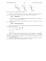
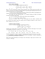
2.19. The left figure is obtained for y0 = 1 . In fact, we see here a fast tending the variable to zero. The right figure shows the y (t ) dependence for, y0 = 0 for a process when sliding changes
its direction several times. The variable is nearly constant at sliding and changes rapidly at sticking. Figures were obtained for the friction ratio d = 1,2 .
(
)
Fig. 2.19. Variable y (elastic deflection) versus time for different initial condition
Note 1. ‘Friction’ and ‘elastic-friction’ force show in simulations similar results. The
‘elastic-friction’ force introduces an additional variable and makes equation of motion stiff. So,
we recommend using the ‘friction’ force.
Note 2. Model of the force contains a first order differential equation, but its internal representation is replaced by an equivalent second order differential equation
c
1
&z& + z& = - sgn(v - &z&) × F , y = z&
d
d
This replacement serves the unification of numerical methods.
Adding a new element of this type to a model see in Chapt.3, Sect. Input of bipolar force
elements | Friction and elastic-friction elements.
2.6.2.4.
Elastic-frictional force 2
The force element is a spring ( c1 ) in series with a parallel combination of the second
spring ( c2 ) and a Coulomb friction element. In contrary to the previous two model of the fric-
Universal Mechanism 5.0
2-36
Part 2. Mechanical system
tional element, here the friction force is not constant. Its value depends on a deflection of the
spring in parallel c2 .
Consider mathematical model of the element. Let x1 , x2 be the length of the springs, and
x2 (0) = 0, x1 (0) = x (0 ) be initial values of these variables. This means that at start of simulation
the second spring c2 has zero length and this position corresponds to its undeformed state.
Let L0 be the length of the spring c1 in an undeformed state. Then the forces produced by the
springs can be computed from the expressions
f1 = - c1Dx1 = - c1 (x1 - L0 ) = - c1 ( x - L0 - x2 ) = - c1 (Dx - x2 ),
f 2 = - c2 Dx2 = - c2 x2 .
Here Dx = x - L0 .
As usual, the friction has two models. At sticking we accept a proportionality of the friction force to the force produced by the spring c2
F fr = -m sgn(x& 2 ) f 2 = -m sgn(x& 2 ) c2 x 2 = -m sgn(x& 2 ) sgn(x2 )c2 x 2 .
where m is the dynamic coefficient of friction. The x 2 deflection can be computed from equality
of two forces: the force in the spring c1 and the sum of friction force and the force produced by
the spring c2
f = f1 = f 2 + F fr ,
i.e.
- c1 (Dx - x2 ) = -c2 x2 - m sgn(x&2 ) sgn(x 2 )c2 x2 ,
and finally
c1Dx
c1Dx
=
,
c1 + c2 (1 + m sgn (x&2 ) sgn(x 2 )) c1 + c2 (1 ± m )
Dx1 = x - x2 .
From the expression for x 2 we obtain that at sliding the variables Dx and x 2 have equal signs at
least for m < 1 . The force value is
c c Dx (1 ± m )
f = 1 2
.
c1 + c2 (1 ± m )
The estimation c1 >> c2 often takes place, which yields
f » c2 Dx (1 ± m ) .
In such cases the friction coefficient is a good approximation for the “relative (effective) friction
coefficient” according to the estimate
f - fs
j= c
»m,
fc + f s
where f c » c2 Dx (1 + m ), f c » c2 Dx (1 - m ) are forces at compression and stretching.
x2 =
At sticking the deflection x 2 is a constant and the resultant force produced by the element is computed from the formula
f = f1 = c2 (Dx - x2 ) ,
Finally, slip-stick transition occurs when the velocity x& 2 changes its sign. The sign of the veloci-
ty is estimated on the difference x2 - x2- , where x 2- is the value of the coordinate at the previous
integration step. Stick-slip transition occurs when
F fr = f1 - c2 x2 > m 0 c2 x2 ,
where m 0 is the static coefficient of friction.
Universal Mechanism 5.0
2-37
Part 2. Mechanical system
List of parameter of the model:
c1 , c2 - stiffness,
m, m 0 - static and dynamic coefficients of friction,
L0 - length of element in an undeformed state.
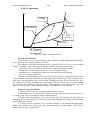
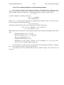
A typical hysteresis (force versus coordinate) as well as coordinate x versus time are
shown in Fig. 2.20. The amplitude of vibrations decreases exponentially like a viscous damper,
but the element realizes a frequency independent damping like rubber.
Fig. 2.20. Force versus coordinate x; coordinate x versus time
Note 1. Force element of this type can by used for modeling leaf springs, internal friction
in rubber elements etc.
Note 2. Element is automatically switched of if at least on of the parameters c1 or c2 is
zero.
Note 3. When friction is zero, the element corresponds to two springs in series.
Note 4. Bipolar force element degenerates at zero length. If it pass through zero length,
the simulation results are incorrect.
Note 5. Do not set coefficient of friction more that 1.
Note 6. Static and dynamic coefficients of friction are usually equal for elements of this
type.
Note 7. At sticking the element has no dissipates. If necessary, add dissipation in parallel
(Sect. List of forces).
Adding a new element of this type to a model see in Chapt.3, Sect. Input of bipolar force
elements | Elastic-friction element 2.
Universal Mechanism 5.0
2.6.2.5.
2-38
Part 2. Mechanical system
Stiffness and damping in series and parallel
Fig. 2.21. Scheme of the force element
The scheme of the element includes linear spring and in series linear spring damping in
parallel (Fig. 2.21, left). This element is used, e.g. in the Nishimura model of an air spring. In a
particular case c1 = 0 (Fig. 2.21, right) the element is a linear spring and damper in series, and
such elements are used for modeling of dampers, as a part of models of rubber, elastomer, etc.
Mathematical model of the element is obtained from equality of elastic and viscoelastic
forces and includes the following differential equation
nx&1 + c1 x1 = c x - x0 - x1 = c Dx - x1 ,
(
) (
)
where x0 is the length of the unloaded element (ignored if c1 = 0 ).
Thus, the element adds a new variable x1 to the model and the corresponding differential
equation. If the time constant
n
T =
c
is small, the differential equation is stiff. In such cases the Park solver with computation of Jacobian matrices is recommended. It is worth to note that if T is small, and the analyzed object motion is slow, the element is equivalent to a simple linear damping with the same damping ratio.
Note 1. Model of the force contains a first order differential equation, but its internal representation is replaced by an equivalent second order differential equation
&z& +
c + c1
n
z& =
c
x
n
This replacement serves the unification of numerical methods.
Note 2. Usually the initial value of x1 variable (more accurately, initial for z and z& ) is
zero.
Adding a new element of this type to a model see in Chapt.3, Sect. Input of bipolar force
elements | Viscoelastic element.
2.6.2.6.
Points model
This type of the force requires the description of the f ( x ) , f (v ) or f (t ) functions in a as
a set of points. Coordinates of points can be both numbers and expressions. UM uses linear interpolation and extrapolation for calculation of force values in an arbitrary point. The figures below show some force models, which can be easily realized with the help of this method.
Universal Mechanism 5.0
2-39
Part 2. Mechanical system
All three models require four points for description.
Adding a new element of this type to a model see in Chapt.3, Sect. Input of bipolar force
elements | Points (numbers), Input of bipolar force elements | Points (expressions)
2.6.2.7.
Expression
The force model is an expression including standard elementary functions. For instance,
f = f 0 - c * ( x - x0 ) - d * v + a * sin (15 * t )
Adding a new element of this type to a model see in Chapt.3, Sect. Data types | Expression – explicit function.
2.6.2.8.
Fancher leaf spring
This type of force is used for simulation of leaf massless springs. The mathematical model of the force is the following:
b
- Dx - Dx
Fi = Fenv,i + ( Fi -1 - Fenv ,i -1 )e i i -1 ,
Fenv,i = -cDx i - F fr sign{Dxi - Dx i -1},
F fr = fcDxi ,
Dx = x - x0 .
Here i is the number of the integration step, f is the friction coefficient, c is the stiffness
of the spring, F fr is friction force, b is the exponential suspension parameter, x0 is the height of
the spring in the undeformed state. Parameters c and f may depend on the spring state: stretched
( dx < 0 ) or compressed ( dx > 0 ).
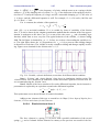
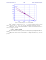
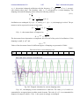
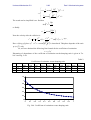
The plot in the figure below shows an example of free vertical vibration of a body connected with the base by the Fancher leaf spring element, b = 0.002 m.
Universal Mechanism 5.0
2-40
Part 2. Mechanical system
Fig. 2.22. Typical behavior of the Fancher model
Note. The model is unstable for big b. If b ® 0 , the model is similar to the force of kind
elastic – frictional 2, see Sect. 2.6.2.4, with equal static and dynamic coefficients of friction.
Adding a new element of this type to a model see in Chapt.3, Sect. Input of bipolar force
elements | Fancher leaf spring.
2.6.2.9.
External function
The function should be written by the user with the help of programming in the UM environment.
Adding a new element of this type to a model see in Chapt.3, Sect. Data types | External
functions.
Universal Mechanism 5.0
2-41
Part 2. Mechanical system
2.6.2.10. Hysteresis
F
Loading
Stop
Start loading
Start
unloading
Unloading
x
Preloading
Fig. 2.23. Scheme of hysteresis curve
Notions and definitions
Force of this type is used for modeling force elements, which mathematical model contains a hysteresis like cushioning device in a train.
The scheme of the force description curves is shown in Fig. 2.23 (force versus element
length or coordinate value). The force description includes definition of four curves:
- preloading, which is a nonlinear elastic curve including possible clearance;
- loading curve, containing two parts: the start loading and loading;
- unloading curve, containing two parts: the start unloading and unloading;
- stop is a nonlinear elastic curve.
The start loading/unloading curves are used in particularly for computation of the curve
of intermediate loading/unloading shown in the figure by the dashed curve. The transition of the
force law to the intermediate curve occurs in the following two cases. First, when the force is on
the loading curve and the coordinate starts decreasing. Second, when the force is on the unloading curve and the coordinate starts increasing. After transition to the intermediate curve, the
force follows it up and/or down until the loading or unloading curves are reached.
Details of curve descriptions
1. The user should enter a set of points, which lie on the curves.
2. Each of the curves is described by numbers of points; abscissas of the points must be in
ascending order. The curves must be single-valued functions.
3. Points connecting different curves must be the same. For instance, the first points on
unloading and start loading curves or the first point on the loading curve and the last point on the
start loading must coincide.
4. A curve can be a polyline (set of straight sections) or an interpolation polynomial,
which order should be set by the user. Note that the number of points setting a line must be
greater than the order of polynomial.
Universal Mechanism 5.0
2-42
Part 2. Mechanical system
Formulas for evaluation of intermediate loading-unloading curve
a
F
Loading
D
V
C
Start loading
b
u
B
Start
unloading
a
U
A
Unloading
x
a
s
s
s
Fig. 2.24. Definition of intermediate loading-unloading curve
Suppose that the transition to the intermediate curve occurs from the loading curve at
point V (Fig. 2.24). The unitless parameter a Î [0,1] is comuped as
x - xC
a= V
x D - xC
Point U on the unloading curve is defined by the same value of the parameter a. Abscissa of
point U is
xV = x Aa + x B (1 - a )
The intermediate curve passes trough points U, V. Let us compute its arbitrary point u, which
abscissa corresponds to the unitless parameter s Î [0,1]
x - xu
.
s= V
xV - xU
Points a, b on the start loading and start unloading curves for the given values of s have the following abscissa values:
xa = x A s + xC (1 - s ), xb = x B s + x D (1 - s ) .
Then abscissa and ordinate of point u are computed according to the formulas
xu = ( xU - x Ba - x A (1 - a ))(1 - s ) + ( xV - x Da - xC (1 - a ))s + xba + xa (1 - a ),
Fu = (FU - FBa - FA (1 - a ))(1 - s ) + ( FV - FDa - FC (1 - a ))s + Fba + Fa (1 - a )
The intermediate curve defined by these formulas has the following properties:
- by a = 0 it coincides with the start loading curve;
- by a = 1 it coincides with the start unloading curve;
- for other values of a it passes through points U, V.
Thus, the intermediate loading/unloading curve is a combination of start loading/unloading
curves.
Universal Mechanism 5.0
2-43
Part 2. Mechanical system
Fig. 2.25. Example of hysteresis model with a soft characteristic
An example of a hysteresis force is shown in Fig. 2.25. The preloading curve is a polyline
passing through three points; it specifies the 10 mm clearance. The loading, unloading and start
unloading curves are set by 3 points each; the second order interpolation polynomials are used.
The start loading curve is specified by two closed points; it is invisible on the plot. Three intermediate curves and the stop curve (straight section) are presented in the figure as well.
Fig. 2.26. Example of friction hysteresis model
Elastic-frictional force with load dependent friction is shown in Fig. 2.26. All curves are
polylines.
Input of the element parameters see in Chapt.3, Sect. Data Input / Input of force elements
/ Input of bipolar force elements / Hysteresis.
Universal Mechanism 5.0
2-44
Part 2. Mechanical system
Remarks
1. Hysteretic elements can work at compression, stretching, and symmetrically in both directions.
2. It is recommended to add a linear dissipative element in parallel with the hysteretic one
because the intermediate curve does not dissipate energy.
2.6.2.11. Impact (bump stop)
Forces of this kind works as bump stops and use the following mathematical model:
D = x-l
, where
F = -cDb - step (D,0, D d ,0, d )v
x is the current length of the force elements for bipolar forces or the current value of joint
coordinate for joint forces;
l is the length of the element at zero clearance when force element starts to work;
c is the stiffness coefficient in a contact;
b is the force curve exponent, is not used in the current version of UM software, assumed
to be 1;
D d is the contact deflection where damping coefficient reaches its maximal value d;
d is a damping coefficient in a contact,
step is a special function, see below for details.
Due to using step function effective damping coefficient changes smoothly from zero at
zero deflection to maximal damping coefficient d at D d deflection.
Description of step function
Step function smoothes switching between two levels of a function Y (Y1, Y2) within
some (X1, X2) interval.
ì y1 , x £ x1
ü
2
æ x - x1 ö æ
2( x - x1 ) ö ï
ï
÷÷ çç 3 ÷ ý, x1 < x < x 2
step ( x, x1 , x 2 , y1 , y 2 ) = í y1 + ( y 2 - y1 ) çç
x 2 - x1 ÷ø ï
ï y , x ³ x è x 2 - x1 ø è
2
î 2
þ
y
Y2
Y1
X1
X2
Fig. 2.27. STEP function
x
Universal Mechanism 5.0
2-45
Part 2. Mechanical system
2.6.2.12. Library (DLL)
Forces of this kind are calculated in an external Dynamic-Linked Library (DLL). It helps
the user to describe any mathematical model of force to include in a considered mechanical system. To develop your own external library the user can use any software environment and any
program language that supports creating Dynamic-Linked Libraries (DLL). Ready-to-use DLLs
for scalar forces of the Library (DLL) type should be placed in the <um_root>\bin\lib\bfrc folder.
Please turn to the Chapt. 5 of UM User’s Manual, Sect. Creating and using external libraries, for detailed guide into developing and using external libraries in UM models.
2.6.2.13. List of forces
List of forces is a set of force elements of above types in parallel. The total force is the
sum of forces produces by separate elements in the list/ The element allows creating useful combinations of forces such as nonlinear damper in parallel with nonlinear spring, rubber-metal elements etc.
Adding a new element of this type to a model see in Chapt.3, Sect. Input of bipolar force
elements | List of forces.
Universal Mechanism 5.0
2-46
Part 2. Mechanical system
2.6.3. Generalized linear force element
When modeling various technical systems, especially those used in transport, force elements linearly depending on the relative displacements of bodies and the velocities of their relative motion are so often to be obtained whereas the influence of their dynamics is insignificant.
A spring and a damper belong to this type of elements. To model such forces automatically UM
uses the generalized linear and damping force elements. An element of this type connects two
different bodies (one of which may be the basic one). One body is considered the first, the other the second.
Let us consider the model of a linear elastic force
element in more details (see the figure). Two bodies are
shown. The A and B2 points of the bodies are connected
by the linear elastic force element. The body-fixed systems of coordinates SC1 and SC2 have O1 and O2 as origins. The element attachment points are set by two vectors r11,r 22 , each of them should be set in the SC of the
corresponding body.
And additional body1-fixed system of coordinates
(SC of the element) has point A as the origin. Axes of
SCA are arbitrary oriented relative to SC1, in a simples
case they are parallel to the axes of SC1.
An additional point B1 is assigned to the first
body. The r112 vector specifies its position in SC1. Point
B1 is the origin of a system of coordinate (SCB1), which
axes are parallel to SCA. Another additional SCB2 is
fixed in body 2, its axes are arbitrary oriented relatively to SC2. Point B1 corresponds to the position of the second end of the force element (i.e. it coincides with B2) when dr vanishes (dr=0).
The relative rotation dp is equal to zero when the axes of SCB1 and SCB2 are parallel.
Thus, the force is equal to the stationary value F0, and the moment vanishes when SCB1
and SCB2 coincide. Displacement of B2 relatively to B1 sets the dr vector, whereas the rotation
of SCВ2 relatively to SCВ1 (SCA) sets the dp vector. Both dr and dp are assumed to be small
and define the force and the moment values.
Now consider the mathematical model of the force element. The force F and the moment
applied to the second body at B2 and resolved in SCB1 (SCA) are:
F = - F0 - C rr dr - C ra dp - Drr v - Dra w,
T
M = -Car dr - C aa dp - Dar v - Daa w
for an viscoelastic, and
F = - Drr v - Dra w,
T
M = - Dar v - Daa w
for a damping element. Here v = dr&, w is the angular velocity of the second body relative to the
first one.
The formulas can be rewritten as:
G = G0 - CdR - DV ,
G = - DV ,
with С and D as the 6 ´ 6 stiffness and damping matrices, and
Universal Mechanism 5.0
2-47
Part 2. Mechanical system
æFö
æF ö
æ dr ö
ævö
G = çç ÷÷, G0 = çç 0 ÷÷, dR = çç ÷÷, V = çç ÷÷
èM ø
è0ø
è dp ø
è wø
Here is the list of parameters describing the element:
- r1 , r12 , r 2 - the coordinates of points A, B1, B2; points A, B1 should be defined in
SC1, whereas point B2 should be defined in SC2;
- orientations of SCA (SCB1) relative to SC1, and SCB2 relative to SC2; in the UM Input Module the oriented connection point are used to define both the point and the orientation of
system of coordinates;
- stiffness C and/or damping D matrices as well as the stationary force F0 (optionally);
these data are defined in SCA (SCB1).
Force element can be also used for modeling a bilinear spring, i.e. a set of two springs
where the internal spring is lower than the external one. The internal springs works when the
longitudinal deflection of the external spring is greater that the difference between the spring
heights. A bilinear element is described by two stiffness matrices and by the height difference.
Generalized linear force element can be only used if relative displacements of interacting
bodies are small.
See Sect. 2.6.6.5. Spring.
Examples of description and/or usage:
- Chapt.7. Sect. Models of Springs;
- \samples\Manchester benchmarks\Vehicle1;
- \samples\wedgetest.
Universal Mechanism 5.0
2-48
Part 2. Mechanical system
2.6.4. Contact forces
2.6.4.1.
Points-Plane and Points-Z-surface types
Fig. 2.28. Point-Plane contact model
UM uses the Points-Plane contact force element for modeling the simplest contact interactions between two bodies (Fig. 2.28). A set of body-fixed points is assigned to the first body
(body 1, a single point C is shown in Fig. 2.28). A body-fixed plane is assigned to the second
body (body 2). The plane is specified by a body fixed point (A) and by an external normal n.
The contact points, point A and normal n should be given in SC of the corresponding bodies.
Number of contact points is unlimited.
Fig. 2.29.
If the distance D between the contact point and the plane is positive and the contact is a
unilateral one, the contact force is equal to zero (no contact, Fig. 2.29 left). If D<0 (Fig.
2.29 right) the force appears. The contact force has two components: the normal force N directed
along the normal n, and the friction force F f situated in the contact plane.
Universal Mechanism 5.0
2-49
Part 2. Mechanical system
Fig. 2.30.
A linear viscoelastic model is used for the normal force
N = - cD - dD× ,
If this value is negative and the contact is a unilateral one, the force is equal to zero (no adhesion). Parameters c, d are constant stiffness and damping coefficients.
There exist two modes for the Coulomb friction low: sliding and sticking. The force
model in the sliding mode is
F f = - fN v s v s ,
where v s is the sliding velocity (projection on the contact plane of velocity of point C relative to
body 2), f is the dynamic friction coefficient. The sliding-sticking transition occurs when the
sliding velocity changes its direction on an opposite one. The program realization compares the
scalar product of the velocity on the current integration step and the velocity on the previous
step. If the product is negative, the sticking occurs, and the friction force on the previous step
Fg and the rg 0 =AD vector are stored, where D is the projection of point C on the contact plane
(Fig. 2.29).
The friction force model in the sticking mode looks like this:
(
)
F f = Fg - c rg - rg 0 - dv s
where rg is the current value of the vector AD. Thus, the point D is connected with the contact
plane by a linear viscoelastic element at the sticking mode. The force Fg in the formula ensures
the continuity of the friction force at the sliding-sticking transition.
The sticking mode is over when the friction force exceeds its maximal value
Ff > f0 N ,
where f 0 is the static friction coefficient, f 0 > f .
The following parameters specify the Points-Plate force element:
· Coordinates of contact points in SC of the first body;
· Coordinates of a point and an external normal to the contact plane in SC of the second
body;
· Parameters characterizing contact forces: dynamic and static friction coefficients, contact
stiffness and damping coefficients c, d .
An additional mode of the contact description is implemented in UM, a so-called mode of
close contact. In this mode, the normal n and/or the point A are determined automatically. The
mode is enabled by the following conditions:
- Number of contact points is greater than 2 (for the normal detection only);
Universal Mechanism 5.0
2-50
Part 2. Mechanical system
-
Contact points lie in a plane (for the normal detection only);
At the moment the simulation starts, the contact point plane (belongs to the first
body) and the contact plane (the second body) are close, i.e. a small clearance d between the planes is allowed. A small deviation of the normal to the planes is allowed
as well.
The close contact description requires specifying the clearance and the normal deviation
Dn . The following actions are made by UM to define the contact plane (the second body):
· The external normal n 2 to the plane is computed as
n 2 = -n1 + Dn ,
where n1 is the normal to the points plane (the first body), Dn is the normal deviation. The n1
vector is determined by three first contact points, entered by the user, according to right-hand
screw rule, the points cannot lie on a line. The normal n1 should be external for the first body
contact (the opposite vector - n1 is assumed to be external to the contact plane of the second
body).
Point A on the contact plane (the second body) is computed according to the formula
rA = r1 + n1d
where d is the clearance, r1 is the vector to the first contact point specified by the user.
Before the simulation of the object starts, the contact plane position is calculated anew
according to initial positions of the bodies.
The contact can be a bilateral one (the contact forces appears independent on the direction or penetration of the point). In this case the clearance can be introduced even if the option of
a close contact is not applied.
Note. Points- Z-surface contact element is mathematically similar to the above one. In
the case of this element, the contact plane is replaced by a surface, which is described by the
functional relation z = f ( x, y ) . No close contact mode is available for this contact.
Universal Mechanism 5.0
2.6.4.2.
2-51
Part 2. Mechanical system
Point-Curve contact
O1
r1
r(p)
O2
Fig. 2.31. Point-curve contact
This type of contact interaction realizes sliding with a small deviation of a point belonging to the first body on a curve, which is fixed relative to the second body, Fig. 2.31.
Position of the contact point relative to SC1 is set by a constant vector r1 .
In general the curve in SC2 is specified by a dependence of coordinates of points on the
curve on a scalar parameter p (the upper index in the equation corresponds to the number of SC)
r 2 = r 2 ( p ), p Î [ pmin , pmax ] ,
where r 2 is the radius vector of a point on the curve in SC2. The equivalent scalar form of the
curve equation is
x 2 = x 2 ( p ), y 2 = y 2 ( p ), z 2 = z 2 ( p ),
r 2 = (x2 , y 2 , z 2 )T
The following classification of curves is used:
· open curve, which end points differ, r 2 ( p min ) ¹ r 2 ( pmax ) ;
· closed curve, end points are equal, r 2 ( p min ) = r 2 ( pmax ) ;
· periodic curve is a closed curve, which have smooth derivative at the end points (tangents
coincide) r¢2 ( pmin ) = r¢2 ( pmax ) ; the stroke here corresponds to derivative with respect
to the parameter p.
a
b
Fig. 2.32. Examples of different curves
Fig. 2.32 shows an open (a), closed (b) and periodic (c) curves.
c
Universal Mechanism 5.0
2-52
Part 2. Mechanical system
Each of the two end points of an open curve can be either locking or unlocking.
The locking end point keeps the contact point on the curve while by passing through the unlocking point the contact disappears.
Singular points are locking end points of an open curve as well as points on it where he
derivative discontinues (jump in the tangent or edge points, see Fig. 2.32 b).
r1
Dr
С
N
F
Fig. 2.33. To model of contact forces in non-singular points
In case of a contact in non-singular points, two contact forces appear: a normal force N
perpendicular to the curve and a tangent friction force F. The normal force vector applied to the
contact point C, Fig. 2.33, is computed by the formula
N = -cDr - nDr&
where Dr is the vector of the minimal deviation of the point from the curve; c and n are the contact stiffness and damping constants.
The friction force supports both sliding and modes similar to the point-plane contact
model.
r1
N
Dr
С
Fig. 2.34. To model of contact forces in singular point
In case of contact in a singular point, Fig. 2.34, the friction force vanishes, and the normal force depends on the vector of deviation Dr of the contact point C from the singular point
according to the above equation.
Remark. If the contact stiffness is big enough, the deviation of the contact point from the
curve is small. Values of contact stiffness and damping constants should be chose according to
recommendations in Sect. 2.7. Methodology of choice of contact parameters, page 2-66.
Universal Mechanism 5.0
2.6.4.3.
2-53
Part 2. Mechanical system
Other types of contact forces
UM allows other types of contact:
· Sphere-Plane;
· Circle-Plane;
· Sphere - Sphere;
· Circle - Z surface
· Sphere - Z surface.
All of these contacts describe rolling one body on a surface of another one.
Consider mathematical models of the contacts. First of all, the minimal distance between
the surfaces is determined. If the distance is positive, contact forces are zero, if not, the normal
force N is computed (Sect.2.6.4.1). The friction force model differs from that in Sect.2.6.4.1:
ì - fN v v , v > v * ,
s
s
s
s
ï
Ff = í
*
v s £ v *s ,
ïî- fN v s v s ,
where f is the dynamic friction coefficient, N is the normal force, v s is the sliding velocity, v *s
is the empirical (small enough) value of sliding velocity. If the sliding velocity as not small, the
classical model of friction is used, else the viscous damping is considered. The v *s value is equal
to 0,01R, where R is the characteristic size (radius) of contacting bodies.
Universal Mechanism 5.0
2-54
Part 2. Mechanical system
2.6.5. 3D contact
The common approach for simulation of contact between rigid bodies based on its contact manifolds defined through graphical objects is implemented in UM 5.0. This approach treats
nondeformable 3D objects with small overlaps at the contact. The presented approach consists of
two parts: a collision detection for arbitrary polyhedrons and then a contact force calculation.
Collision detection deals with generalized three-dimensional clipping algorithm by Cyrus and
Beck [2]. Contact force calculation is based on a point-plane model and computed as a sum of
normal viscous-elastic and tangential dry friction forces. Several examples of application of this
approach for simulation of multibody system dynamics are given.
Collision Detection for Polyhedrons
To accelerate computational processes the collision detection is typically divided into socalled far and near collision detection problems. Far collision detection is usually a fast algorithm that should select polyhedrons for the following, usually more time-consuming, near collision detection. On the first stage of the far collision detection circumscribed spheres around polyhedrons are created and its intersection is checked. The polyhedrons that passed through the far
collision detection are treated by a near collision detection algorithm.
The well-known in computer graphics generalized three-dimensional clipping algorithm
by Cyrus and Beck is used as the near collision detection algorithm. The algorithm deals with
two convex polyhedrons and gives as a result clipped edges of one polyhedron that lie within
another one and vice-versa, see Figure below. For example, the algorithm gives the set of edges
{E1, E2, E3} of Body2 and the empty set of edges for Body1 in Fig. 2.35a and {E1} of Body1 and
{E2} of Body2 in Fig. 2.35b.
Body2
Body2
Body1
Body1
a)
b)
Fig. 2.35. Vertex-face and edge-edge penetration
Contact force calculation
After all collisions between the neighboring polyhedron pairs have been detected, the
contact forces have to be determined. Let us consider a pair of polyhedrons. Having a set of
clipped edges that belong to each polyhedron the algorithm of calculation of contact forces arranges contact points on each edge, see Fig. 2.36a. The step size between neighboring contact
points is a parameter of the mathematical model that depends on a characteristic dimension of
polyhedrons. Then for each contact point the nearest face on another polyhedron from the pair is
determined. As soon as pairs of points and planes (faces) are obtained the contact force R can be
calculated as a superposition of normal viscous-elastic force N , depending on penetration Δ and
its derivative, and tangential dry friction force F f , see Fig. 2.36b, [2].
Special control procedure keeps position of contact points on an edge during a contacting
phase even the length of clipped part of the edge is changed. Such strategy provides smooth
changing a resultant vector of contact force between two bodies with time.
Universal Mechanism 5.0
2-55
Part 2. Mechanical system
Body2
Body2
Body1
Body1
a)
b)
Fig. 2.36. Contact points and forces
The presented approach perfectly manages both basic contact situations: vertex-face and
edge-edge penetrations, Fig. 2.35. Since the Cyrus and Beck algorithm deals with convex polyhedrons, the presented approach for contact force simulation is also applicable for a case of convex polyhedrons only. However the suggested algorithms can be enlarged for non-convex case if
non-convex polyhedrons would be preliminarily divided into convex ones. In practice this strategy works well when a convex decomposition is available with a moderate number of pieces, it
breaks down for utterly non-convex objects.
2.6.6. Special forces
The following types of force elements are implemented in UM as special forces:
· Gearing;
· Combined friction;
· Cam;
· Spring.
2.6.6.1.
Gearing
The gearing is realized in UM as a simplified model of contact iterations of gears. The
force model can be used for simulation of plane gear (internal and external) and bevel gearing
taking into account possible clearance between teeth as well as a compliance reduced to the contact point.
The gearing is specified by the following parameters (Fig. 2.37):
· two points A and B on the gear axes coinciding with the gear centers (coordinates
should be given in body-fixed frames);
· two unit axle vectors (in body-fixed frames);
· gearing ratio (radius of the first gear R1 divided by the radius of the second one R2);
· clearance d;
· gearing stiffness coefficient reduced to the contact point c (N/m);
· gearing damping coefficient reduced to the contact point d (Ns/m);
· type of gearing internal or external, for plane gearing only.
Gear radii are calculated by UM automatically.
Fig. 2.37.
Universal Mechanism 5.0
2-56
Part 2. Mechanical system
The gearing is modeled by a tangential force at the contact as
ì - c (D - d 2 ) - dD& , D > d 2
ï
F = í- c (D + d 2 ) - dD& , D < - d 2 ,
ï
0, D < d 2
î
D = R2j 2 ± R1j1 .
Here the force acts on the second body (the opposite force acts on the first one). j1,j2 are the
angles of gear rotations. The minus sign in D corresponds to an external gearing.
Remarks.
1. The gear axes must lie in a plane.
2. Use the Initial conditions tab of the Object simulation inspector to compute initial velocities before the simulation starts (Chapt.4).
Universal Mechanism 5.0
2.6.6.2.
2-57
Part 2. Mechanical system
Rack and pinion
Rack and pinion force element is a special case of gearing described above (see in
Sect. 2.6.6.1). The only difference is that the second body (rack) moves translational.
Universal Mechanism 5.0
2.6.6.3.
2-58
Part 2. Mechanical system
Combined friction
The force is a combination of a normal force N directed along the axis of the element and
a perpendicular friction force, which in the sliding mode is F = mN . The normal force is a
function of the element length x, its time derivative v ant t, types of function are described in
Sect. Types of scalar forces. The friction force has both sticking and sliding modes. In 2D model
of the element the friction force directed along a line fixed to body 1, in 3D case the friction
force lies in a plane.
N
D
Body2
F
Massless body
Body1
Fig. 2.38. Scheme of the combined friction
In the 2D case the force model can include a fictitious massless third body and a clearance D, Fig. 2.38.
2.6.6.4.
Cam
Fig. 2.39. Types of cam models
The special case of contact interaction is an interaction of a cam and a piston or a link.
The mathematical model of this interaction is similar to one described above (Sect. Points-Plane
Universal Mechanism 5.0
2-59
Part 2. Mechanical system
and Points-Z-surface types). Types of cam-piston (cam-link) couples and examples of their using
are shown in the Fig. 2.39.
Three types of cam pairs are implemented in UM depending on the contact type:
· point (the first figure);
· roller (2nd and 5th figure);
· plane (3rd and 4th figure).
The Coulomb (dry) friction is taken into account for the plane and point contact types,
whereas the roller contact is considered as an ideal one (without friction).
Note. There is only one contact point at each moment of time. In the multipoint case actually the point with the maximal penetration is considered.
The examples of the description and/or usage:
- Chapt.3. Sect. Cam
- \Samples\cams
Universal Mechanism 5.0
2.6.6.5.
2-60
Part 2. Mechanical system
Spring
Special force element Spring is a special case of a general linear force element
(Sect.2.6.3), which is used for modeling linear helical springs with equal shear stiffness in any
direction perpendicular to the spring axis and with the symmetric rigid fixing of ends. It is supposed also that the spring axis is parallel to one of the axes of the first body-fixed system of
coordinates.
Stiffness matrix, which is introduced in Sect. 2.6.3, for a spring parallel to Z-axis of the
body1-fixed SC, has the following form:
0
0
0
- cs H 2 0 ö
æ cs
÷
ç
0
0 cs H 2
0
0÷
cs
ç
ç
0
0
0
0
0÷
cl
÷
C=ç
0
0
0÷
cs H 2 0
cj
ç
ç- c H 2
0
0
0
0÷
cj
÷
ç s
÷
ç
0
0
0
0
0
c
aø
è
Here c s , cl , cj , ca are shear, longitudinal, bending and torsion stiffnesses of the spring, H is the
length of the spring. As a rule the length H for vertical springs takes into account the static load.
dy
Body2
F
m
z
H
y
x
F
m
Body1
Fig. 2.40. Spring forces
Let us consider how we can get the values for non-diagonal elements of this matrix. Let
the second body be over the first one. Shift body 2 along Y-axis on dy, Fig. 2.40. The force
F y = - c s dy appears. An opposite force acts on the upper end of the spring and the same force
acts on the lower end. Equilibrium of the spring requires a balancing pair of forces with the moment c s dyH . This pair must be realized by two equal (due to symmetry) pairs c s dyH / 2 in the
upper and lower ends. Thus, the moment with the X-projection - c s dyH / 2 acts on the second
body, which results in the non-diagonal element of the stiffness matrix
C42 = cs H / 2
as well as in the element C 24 which is equal to C 42 due to symmetry of the matrix. Elements
C52 = C 25 can be obtained analogously.
Universal Mechanism 5.0
2-61
Part 2. Mechanical system
If the spring is parallel to the Y-axis, its stiffness matrix is
0
0
0
0 ± cs H 2 ö
æ cs
÷
ç
0
0
0
0
0
cl
÷
ç
÷
ç
0
0
0
m cs H 2 0
cs
÷.
ç
C=
0
0 m cs H 2
0
0
cj
÷
ç
÷
ç
0
0
0
0
0
ca
÷
ç
÷
ç ± cs H 2 0
0
0
0
c
j
ø
è
This matrix is obtained from the previous one permutations x ® z , y ® x, z ® y. Finally, here
is the matrix for a X-parallel element.
0
0
0
0
0
ö
æ cl
÷
ç
0
0
0
m cs H 2 ÷
cs
ç0
÷
ç0
0
0 ± cs H 2
0
cs
÷
C=ç
0
0
0
0
ca
÷
ç0
÷
ç0
0
0
cj
± cs H 2 0
÷
ç
÷
ç 0 m cs H 2
0
0
0
c
j
ø
è
Coefficients of stiffness c s , cl , cj for this type of force elements can be computed automatically according to spring height, radius, number of coils etc.
Note. If it is necessary to describe a spring, which is not parallel to one of the body1fixed axis, a special fictitious body should be introduced. This body must be fixed to body1 one
of its coordinate axis must have the desirable direction. Joint fixing the fictitious body and body1
can be a generalized joint, which allows constant rotations as elementary transformations
(Sect.2.3.2.3), and can provide any orientation of the fictitious body relative to body1.
Examples of description and/or usage:
- Chapt.7. Sect. Models of Springs
- \samples\rail vehicles\ac4
Universal Mechanism 5.0
2.6.6.6.
2-62
Part 2. Mechanical system
Bushings
Element of this type is used for modeling linear and nonlinear compliant joints (bushings).
Body2
Body1
r2
r2
B
r1
A
r1
Fig. 2.41. Systens of coordinates of a bushing
Consider the mathematical model of a bushing. Let us introduce two systems of coordinates. The first system SCB1 is fixed relative to body 1, the second one SCB2 is fixed relative to
body 2. Vectors r1,r 2 and constant rotation matrices AB1 , AB 2 determine the positions of
SCB1 and SCB2 relative to the bodies.
It is supposed that deviation of SCB2 relative to SCB1 is small.
In general the mathematical model of the bushing as a force element is expressed in terms
of the displacement of point B relative to SCB1
Dr = r2 + r 2 - r1 - r1
and the direct cosine matrix, which sets the orientation of SCB2 relative to SCb1
AB1B 2 = ABT1 A10 A02 AB 2
This matrix is nearly the identity one for small deviations of SCB2 from SCB1. In this
case a vector of small rotation of SCB2 relative to SCB1 can be introduced as
æ Dp x ö
ç
÷
Dp = ç Dp y ÷ .
ç Dp ÷
è zø
Components of this vector correspond to small rotation angles of SCB2 about axis of SCB1.
The skew-symmetric matrix corresponding to the rotation vector depends on the direct
cosine matrix according to the formula
æ 0
- Dp z Dp y ö
÷ AB1B 2 - AT
ç
~
B1B 2 .
0
Dp = ç Dp z
- Dp x ÷ =
2
÷
ç
0 ø
è - Dp y Dp x
This expression is used for evaluation of the rotation vector by the simulation.
Universal Mechanism 5.0
2-63
Part 2. Mechanical system
Linear model of bushing
In case of a linear bushing its mathematical model is:
æ F B1 ö æ F0 ö
æ v12 ö
æ Dr - Dr0 ö
ç
÷=ç
C
D
÷
çç
÷÷
÷
ç
ç Dp - Dp ÷
ç M B1 ÷ çè M 0 ÷ø
0ø
è w12 ø
è
è
ø
Here F B1, M B1 are the force and the torque produced by the element expressed in SCb1 and
reduced to point B. The following constant parameters specifying the bushing model must be set
by the user (all vectors are resolved in SCB1):
- C and D are the constant diagonal matrices, which specify stiffness and damping constants by movement/rotation along/about axes of SCB1;
- the vectors Dr0 , Dp 0 set small offset, i.e. a ‘constant’ deviation of CSB2, for instance
in stationary position of the model;
v12 = Dr& is re velocity of the SCB2 origin relative to the second body;
w12 = w2 - w1 is the relative angular velocity;
F0 , M 0 are constant values of force and torque for zero relative velocities and
Dr = Dr0 , Dp = Dp 0 ; these vectors are usually used for setting the stationary or static values of
forces, often by Dr0 = 0, Dp 0 = 0 .
Nonlinear model of bushing
In case of a nonlinear bushing its mathematical model is:
æ F B1 ö æ F0 ö æ Fe ö
æ v12 ö
ç
÷=ç
D
÷
÷
çç
÷÷
ç
÷
÷
ç
ç
ç M B1 ÷ è M 0 ø è M e ø
w
12
è
ø
è
ø
Nonlinear part of the model is concentrated in dependence of the force and torque Fe , M e on the
corresponding components of vectors Dr - Dr0 , Dp - Dp 0
Fex = Fex ( Dx - Dx0 ), Fey = Fey (Dy - Dy0 ), Fez = Fez ( Dz - Dz0 ),
M ex = M ex ( Dp x - Dp0 x ), M ey = M ey ( Dp y - Dp0 y ), M ez = M ez ( Dp z - Dp0 z )
Nonlinear dependencies of these components on displacements must be set by the user as plots.
In particular, a nonlinear bushing is often used for modeling or contacts with gaps on
translational and rotational degrees of freedom.
Input of the element parameters see in Chapt.3, Sect. Data Input / Input of force elements / Special forces / Bushings.
Universal Mechanism 5.0
2.6.7.
2-64
Part 2. Mechanical system
T-forces
The element defines a force and a moment, which components are either explicit functions of time or functions of time stored in columns of a text file (the first column contains time).
Remark. The user can introduce additional applied forces acting on bodies in the control
file without describing the forces in the Input module.
Universal Mechanism 5.0
2-65
Part 2. Mechanical system
2.6.8. Force element response in the frequency domain
Force element response in the frequency domain is a useful utility for a scalar force (a bipolar force element or a joint force). Consider a scalar force element, which dependence on a
scalar variable x and its time derivative v is the following (Sect. Types of scalar forces):
F = F ( x, v ) .
Consider a harmonic excitation of the force
x (t ) = x0 + a sin (2 pft )
,
v (t ) = 2pfa sin (2pft )
where x0 , a , f are the center of excitation, its amplitude and frequency in Hz, t is the time variable. The response is the periodic function
F (t ) = F ( x (t ), v (t )) .
Expand this function into Fourier series keeping zero and first order terms
F (t ) » F0 + FK ( f ) sin (2pft ) - FC ( f ) cos(2 pft ) =
= F0 + F1 ( f ) sin (2pft - d( f )).
Main characteristics of the force in the frequency domain are introduced according to this expansion:
- Dynamic stiffness K ( f ) = FK ( f ) a
- Equivalent damping C ( f ) = FC ( f ) (2pfa )
- Phase or damping angle d( f )
- Amplitude of the response F1 ( f ) .
- Dependence of the response function on the coordinate F ( x, v (x )) and velocity F (x (v ), v ) for a fixed excitation frequency.
For description of a tool for force element analysis in the frequency domain see Chapt.4,
Sect. Force element response in the frequency domain.
An example for a force element analysis can be found in Chapt.7, Sect. Elastic-friction
element 2.
Universal Mechanism 5.0
2-66
Part 2. Mechanical system
2.7. Methodology of choice of contact parameters
Contact stiffness c and damping m parameters are used in description of a number of
force elements (Sect. Contact forces, Friction force, Elastic-frictional force, Cam). Let us consider some methods for estimation their numeric values.
The real contact stiffness due to elastic deformations in contacts is usually very high (say,
11
10 N/m). It is clear, that for reasonable values of contacting body masses such stiffness introduces a very high frequency in the model (about c m , where c is the stiffness, and a m is the
mass). This makes the model oscillatory stiff and increases CPU expenses considerably due to
decreasing the integration step size. In practice much less values the stiffness can be set in the
model. Consider the main reasons for that.
Applied theory of ordinary differential equations states (a strict proof can be obtained
with the help of theory of singular degenerate equations) that if a system has two groups of frequencies of different order, e.g. 1–10Hz in the first group and 200–1000Hz in the second one,
the high frequency processes does not affect practically the low frequency processes. Moreover,
changing parameters, which determine high frequency processes, does not lead to considerable
changes of the low frequency processes. That means, if the stiffness c is ‘large enough’, its further increase does not affect analyzed processes, if they are ‘slow’. The stiffness is ‘large
enough’ if the introduced local frequencies are at least by order of magnitude greater than the
frequencies of analyzed object. The frequency k introduced by the contact stiffness may be estimated by the formula k = c m , where m is the lower mass of interacting bodies. Thus, if the
user choose a ‘large enough’ local contact frequency f = k (2 p) Hz, the corresponding contact
stiffness can be computed according to the formula
(2.9)
c = 4p 2 f 2 m .
Consider an example. Let m = 20 kg, f = 200 Hz (i.e. the main frequencies of the object
are 1–10 Hz). Then c = 3.16 ´ 107 N/m.
A stiffness coefficient computed according to this methodology should be verified and
corrected by the user. To do this, run simulations for different values of the stiffness and plots of
object performance variables should be compared. If 2÷10 times increasing the coefficient does
not affect the results, the stiffness is ‘large enough’. In this case it is recommended to try decreasing its value. This may reduce CPU expenses. The boundary of the parameter is its value
when the plots of performances are changed.
Let us discuss now methodology for choosing a dissipation coefficient m . If this coefficient is ‘too small’, high frequency undamped oscillations may appear in the model, which introduce large accelerations. Moreover, frequencies of these oscillations according to the methodology above have nothing in common with the reality. If the damping is ‘too large’, the equations
of motion become stiff, and CPU expenses increase. A correct choice of the damping coefficient
is especially important for systems with unilateral constraints, i.e. for systems with gaps and impacts, because the damping is responsible for a value of coefficient of restitution. Finally, the
value of the damping must correlate with the value of the contact stiffness.
To get a justified value of the contact damping, a very important notion of damping ratio
of critical b and a damping factor b* is used. To clarify this notion consider the equation of free
linear damped oscillations
(2.10)
m&x& + mx& + cx = 0 ,
As it is well known, the solution of this equation depends on ratio of two parameters: the frequency of free undamped oscillations k = c m and the damping coefficient n = m (2m ) . If
Universal Mechanism 5.0
2-67
Part 2. Mechanical system
n < k , the motion is damped oscillations with the frequency k * = k 2 - n 2 . If n ³ k , an aperiodic solution takes place. The boundary value n = k corresponds to a critical damping. The
damping ratio and the damping factor satisfy the following relations
(2.11)
n
b= ,
k
n
n
b* =
=
Î [0, ¥],
*
k
k 2 - n2
Oscillations are undamped if b = b* = 0 , and by b = 1 ( b* = ¥ ) the damping is critical. The parameters can be expressed in terms of each other,
b* =
b
b*
> b, b =
1 + b*2
1 - b2
If b < 1 , a decrement factor is computed as
*
-
pb
D = e - pb = e 1-b .
The decrement factor determines an amplitude fall on a half of the period of oscillations. If the
damping is small, b » b* and
2
D » e - pb .
Values of the decrement factor for different degrees of damping are presented in Table1.
Table 1
Decrement factor versus damping ratio
b
0
0.1
0.2
0.3
0.4
0.5
0.6
0.7
0.8
0.9
1
D
1
0.729
0.527
0.372
0.254
0.163
0.095
0.046
0.015
0.0015
0
Fig. 2.42. shows solutions for different b .
Fig. 2.42. Damped vibrations for various damping ratios
If b £ 0.1 , the damping is often considered as a small one. The value b = 0,1 can be recommended for an approximate in rubber-metal elements. The value b = 0,3 is recommended for
dampers of transport vehicles. If b ³ 1 , the system is strongly overdamped.
Universal Mechanism 5.0
2-68
Part 2. Mechanical system
The above analysis clarifies the notions ‘too small’ or ‘too large’ damping coefficient.
We recommend the damping b = 0,1 ¸ 0,4 for the contact forces. Thus, if you choose some values for stiffness and damping ratio, the coefficient of damping is computed according to the following formula
(2.12)
m = 2b mc .
For the above example c = 3.16 ´ 107 N/m with the damping ratio b = 0,2 we get m » 104 Ns/m.
The next important problem is, how collisions may be likely modeled? If we answer this
question, we could find a more proved value of damping ratio b in cases of unilateral contacts.
Is it is known, one of the most simple and frequently used model of a collision of bodies
is based on the Newton’s coefficient of restitution e, which can be illustrated by the following
example. Consider a mass point, which strikes against a fixed plane. The point velocity before
the collision be v - , and after the collision - v + . The coefficient of restitution is
e=
v+
v-
.
Fig. 2.43. Collision process
Consider the model of viscoelastic interaction of the point with the plane (Sect. 2.6.4.1).
The coordinate x in Fig. 2.43. is the penetration, which determines the normal contact force
N x = -cx - mx& .
During the process of the contact the point motion is described by the differential equation (2.10)
with the following initial conditions: x (0 ) = 0, v (0) = v - . At the compression stage of the collision the normal force increases, and at the relaxation phase it decreases. At some moment t the
normal reaction vanishes and the impact process is over. This, v (t ) = v + .
To get the velocity after the impact, consider the solution of Eq. (2.10)
( )
v - - nt
x=
e sin k *t ,
*
k
æ n
ö
v = v - e - nt ç sin k *t + cos k *t ÷.
*
è k
ø
At the end of the collision we have
ö
æ n
æ
n 2 ö÷
0 = N (t ) = mv (t ) + cx (t ) = m 2nv (t) + k 2 x (t ) = v - e - nt mk * ç 2 sin k *t + ç1 cos k *t ÷ ,
ç
÷
ç k*
k *2 ÷ø
è
ø
è
so the collision duration t satisfies the equation
( )
(
)
( )
tg k *t =
or
( )
( )
2b*
b*2 - 1
( )
Universal Mechanism 5.0
2-69
Part 2. Mechanical system
ì
æ 2b * ö *
1
÷, b < 1
ïp + * arctanç *2
ç
÷
k
ï
è b - 1ø
t=í
*
ï 1 arctanæç 2b ö÷, b* ³ 1
ï k*
ç b *2 - 1 ÷
è
ø
î
The result can be simplified is we find that
( )
sin k *t =
2b 2
b*
or finally
t=
æ 2b 2 ö
÷
arcsin ç
ç b* ÷
k*
è
ø
1
Now the velocity after the collision is:
( )
* +
k2
v - k 2 - nt
e
x (t ) =
sin k *t = v - e -b j .
2n
2nk *
Here a lifting off phase j + = k *t = arcsin 2b 2 b * is introduced. This phase depends of the ratio
v + = v (t) =
(
)
b (or b* ) only.
So, we have obtained the following fine formula for the coefficient of restitution:
*
+
e = e -b j
Illustration of dependance of the coefficient of restitution on the damping ratio is given in Table 2 and Fig. 2.44.
Table 2
b
e
b
e
Coefficient of restitution versus damping ratio
0
0.05
0.1
0.15
0.2
0.25
0.3
0.35
0.4
0.45
0.5
1
0.55
0.859
0.6
0.744
0.65
0.65
0.7
0.572
0.75
0.506
0.8
0.451
0.85
0.404
0.9
0.364
0.95
0.329
1
0.298
0.272
0.249
0.228
0.21
0.194
0.18
0.167
0.155
0.145
0.135
1.2
1
0.8
0.6
0.4
0.2
0
0
0.1
0.2
0.3
0.4
0.5
0.6
0.7
0.8
0.9
Fig. 2.44. Coefficient of restitution versus damping ratio
1
Universal Mechanism 5.0
2-70
Part 2. Mechanical system
If the user knows the coefficient of restitution, he can estimate the damping ration b and,
respectively, the damping coefficient m .
2.8. Subsystems
2.8.1. Subsystem technique
If a mechanical system containing hundreds or thousands of bodies is modeled, the equations of motion are so huge that problems with their compilation might arise. For such a system
the subsystem technique is convenient. In this case, the MBS is preliminarily (conditionally) divided into a few parts - subsystems - and is called a compound object. Separate subsystems may
or may not be connected with each other by joints or force elements.
The subsystem technique is especially effective when several subsystems are kinematically identical or, in other words, have the same kinematical scheme. Here is a rigorous definition of kinematic identity.
Two subsystems are kinematically identical if, their configuration being arbitrary, it is
possible to bring them into spatial coincidence in the basic SC by means of the following transformations:
· translation (the vector is constant);
· rotation about any axis by a constant angle;
· changing of the parameters of the kinematic pairs (e.g., changing the lengths of the members);
· changing the values of the local joint coordinates.
Compound object
External SS
Included SS
External SS
External SS
Included SS
Included SS
Bodies,joints....
Bodies,joints....
...
...
Bodies, joints...
For the equations of motion of the kinematically identical subsystems to be the same the
following conditions should be satisfied: all the constant parameters (masses, lengths of the
structural elements, etc.), which may vary numerically must be represented in a symbolic form
(i.e. by identifiers). While modeling motion, different values may be attributed to the parameters
of different subsystems.
UM model of an object can be structured as a tree of external and included subsystems.
An External subsystem is generated by any preliminarily created UM object - ancestor.
All modifications made in description of the ancestor are automatically taken by all external subsystems – descendants. Moreover, modification in an external subsystem can be made exclusive-
Universal Mechanism 5.0
2-71
Part 2. Mechanical system
ly through modification of the corresponding ancestor. A compound object, which contains external subsystems, does own neither structure, nor parameters of external subsystems, but refers
to them. At the same time, the compound object can add joints and force elements connecting
bodies from different subsystems. Thus, in the case of kinematically identical subsystems, the
user can create an ancestor, generate the equation library for it (dll), and add the ancestor to the
object as many times as it is necessary.
Included subsystems, unlike the external ones, belong to the compound object. The object owns their structures (bodies, joints, forces, etc.) and parameters. Several included subsystems generated by one ancestor can be arbitrary modified. Equations of motion for included subsystems are generated as a part of the object equations.
Subsystems have a tree structure. An object can contain any number of subsystems (both
external and included). Each of the subsystem, in its turn, may be a compound object containing
subsystems.
The subsystem technique is the foundation for development data basis for modeling different technical systems (such as rail vehicles).
2.8.2. Standard subsystems
Standard subsystems are automatically generated subsystems, which are basis for creation of models of technical systems taking their features. Standard subsystems are used in the
main um modules UM: simulation of rail vehicles, automotive vehicles, caterpillar models, and
ballast.
2.8.2.1.
Wheelset as standard subsystem
A standard subsystem wheelset is the base of the UM Loco module for simulation of
railway vehicles. Simultaneously to an automatic adding wheelsets to vehicle models, UM computes rail-wheel contact forces as well as special interface abilities are available with this module.
2.8.2.2.
Vehicle suspensions
UM-automotive module is based on a number of vehicle suspensions.
Universal Mechanism 5.0
2.8.2.3.
2-72
Part 2. Mechanical system
Caterpillar
The UM/Caterpillar module is based on a standard subsystem “caterpillar”, which allows
the user to get a model with any number of tracks, supporting wheels, etc.
2.8.2.4.
Ballast
Generated subsystem ‘ballast’. Simulation of the ballast backfilling process
The ‘ballast’ subsystem is developed for analysis of dynamic properties of broken stone
ballast. The UM ballast model can include thousands of bodies of different shape.
2.8.3. Examples of compound objects
2.8.3.1.
Dynamically independent subsystems
If it is necessary to compare in one time scale the behaviors of the same object in different situations or various objects, the method of subsystems is also useful. In this case, the compound object containing several subsystems generated by one or many UM objects is formed.
For instance, two Puma robots or one Puma robot and a Stanford manipulator can be dealt with
as compound objects (see the \Samples\Robots example). Here, the subsystems are not dynamically connected. However, the integration of equations of motion is done for both subsystems
simultaneously, and the results are displayed out in the same time scale.
Universal Mechanism 5.0
2-73
Part 2. Mechanical system
The number of dynamically independent subsystems in a compound object is limited only by the resources of the user’s PC.
2.8.3.2.
Dynamic platform as a compound object
a)
b)
c)
Fig. 2.45. Subsystem technique
Consider a technical system - a six d.o.f. platform for dynamic tests (Fig. 2.45a, see the
\samples\mechanisms\platform example as well). Modeling its dynamics is no problem without
using the method of subsystems. This example, however, can easily show some distinctive features of the method.
Separate the mechanism into seven subsystems by cutting the joints connecting the six
control mechanisms with the platform. The control mechanisms are kinematically identical and
are generated by the only UM object (Fig. 2.45b). The second simple object is the platform (Fig.
2.45c). The simple object of the control mechanism has one external joint. In Fig. 2.45a the
shown SC is the basic global one of the compound object, whereas in Fig. 2.45b and Fig. 2.45c
the shown systems correspond to the local basic systems of coordinates. When assembling separate subsystems into a compound object the local coordinate systems of the control mechanisms
must be translated and rotated so that the joints connecting the structure elements with the fixed
member could occupy the necessary position. The local SC of the platform is brought into coincidence with the basic SC of the compound object.
Universal Mechanism 5.0
2.8.3.3.
2-74
Part 2. Mechanical system
Locomotive as a compound object
The model of the TE116 locomotive as a compound object consists of a body and two included subsystems – bogies. A bogie contains three included subsystems – wheel-motor blocks,
one body (a bogie frame), and elements of the secondary suspension (springs and dampers). A
wheel-motor block consists of one included subsystem (a wheelset is the standard UM subsystem), a motor, elements of the primary suspension (springs, dampers, propulsion rods), gearing.
The subsystem tree has four levels.
Universal Mechanism 5.0
2-75
Part 2. Mechanical system
TE116
First bogie
1st w/m
block
Wset1
2nd w/m
block
блок
Wset2
Second bogie
3rd w/m
block
блок
4th w/m
block
блок
5th w/m
block
блок
6th w/m
block
блок
Wset3
Wset4
Wset5
Wset6
The model description has three stages.
Stage 1. Creation of an object-ancestor: wheel-motor block, which contains a wheelset as
an included subsystem.
Stage 2. Creation of an object-ancestor: a bogie, which includes three wheel-motor block
subsystems.
Stage 3. Creation of the locomotive object, which includes two bogie subsystems.
Each of the included subsystems is available for separate modification.
2.8.3.4.
Multibody physical pendulum
Consider a chain of similar bodies connected by joints with one rotational d.o.f. The
chain is attached to the immovable support and can move in the vertical plane owing to gravity.
If the number of bodies does not exceed three or four dozens, modeling such a system is easy. If
the number of bodies is greater, the symbolic equations of motion grow huge and this might
cause problems with their compilation.
Apart from the growth of the equation size there exists also the problem of the object description. If to tackle it traditionally, one has to introduce the inertial parameters for each body
and describe all the joints, which is very time-consuming. How then can the motion of, say, a
100-body pendulum be modeled? Cut the chain into ten similar 10-body pendulums, in other
words, into ten subsystems. All of them are kinematically identical, since they are generated by
one ancestor - a 10-body pendulum. The given ancestor has ten bodies and eleven joints: one external and ten internal. The external joint serves as a means to connect the subsystems with one
another in a chain. Nine internal joints connect the bodies of the pendulum, whereas the tenth has
three d.o.f. and is used for the description of the position of one body of the ancestor (e.g. the
fifth one) relative to the SC0.
Since the compound object - the 100-body pendulum - is generated by only one ancestor,
data input and the equations synthesis are carried out only for a 10-body pendulum, which is
easy. The compound object is built then by ten subsystems generated by one ancestor.
Universal Mechanism 5.0
2-76
Part 2. Mechanical system
2.9. Linearization of equations and equilibrium positions
2.9.1. Equilibrium equations and their solving
Consider equations of motion for a multibody system with stationary constraints. If the
system has closed loops, its equations of motion are (2.1):
M (q )q&& + k (q, q& ) = Q (q, q& ) + G T (q )l ,
g (q ) = 0
At equilibrium by q& = 0, q&& = 0 , the following equations take place:
(2.13)
Q (q,0) + G (q )T l = 0 , g ( q) = 0
Here we have nonlinear algebraic equations relative to unknown values of coordinates q=q0 and
Lagrange multipliers l = l 0 . The Newton-Raphson method is used for solving the equations.
The following linear equations are solved at each the iterations:
(Qq (q0k ,0) + F(q0k , lk0 ))Dq0k +1 + G(q0k )T lk0+1 = 0 ,
G ( q0k )Dq0k +1 = - g (q0k ) = 0 ,
q0k +1 = q0k + RDq0k +1
Here Qq is the Jacobian matrix Qq = ¶Q ¶qT , the matrix F is defined by the relation
F = ¶(G T l ) ¶qT ,
R £ 1 is the relaxation factor, which is usually equal to 1.
The iterations are considered as successfully converged if the discrepancies in Eqs.(2.13)
satisfy the condition
å di < e ,
with an error tolerance e .
User’s set initials q00 = q 0 are used as a starting approximation. The Jacobian matrices
Qq ( q0k ,0), F ( q0k , lk0 ) are evaluated by finite differences as
(
)
Qqi ( q0k ,0) = Q ( q0k + dqi ,0)T - Q ( q0k ,0)T d ,
(
)
F i (q0k , lk0 ) = G ( q0k + dqi )T - G ( q0k )T lk0 d .
Here Qqi , F i are the columns i of the corresponding matrices, d is a small real number; the column dqi has one nonzero value at position i, which equals to d.
2.9.2. Natural frequencies, modes, eigenvalues and eigenvectors
QR algorithm is used for computing both natural frequencies and eigenvalues. Reverse
iterations are applied to get modes and eigenforms of linearized equations.
2.10.
Units of measure
In UM all the calculations are carried out in the International System of Units: kg, m, s.
While solving dynamic problems using other units is not recommended (cm, kN, etc.). In the data input unit angles are usually introduced in degrees (when describing initial conditions and limits), whereas when modeling motion their numerical values are obtained in radians.
Universal Mechanism 5.0
2.11.
2-77
Part 2. Mechanical system
Generation and analysis of equations of motion
Kinematical expressions and the motion equation generation of an object are done in a
symbolic form with the help of a built-in specialized computer-algebra system. This decreases
the number of operations for calculating their terms when numerically modeling motion. To decrease the number of operations more significantly fracturing and substituting procedures are
used. The equations are generated either in a non-linear form or are linearized near the stationary
motion.
The equations of motion of a system are generated according to the Newton-Euler formalism and are differential-algebraic. The equations analysis is carried out by means of the
ABM, BDF numerical multistep methods with the automatic choice of the step size and the order
of the method, as well as the Park and Gear methods for stiff equations. While integrating the
equations computing kinematical characteristics and constraint reaction forces is possible.
The Park and Gear methods with computing of Jacobian matrices are recommended for
solving stiff differential-algebraic equations of motion.
The obtaining of equilibrium positions of non-linear objects and the linearization of the
equations of motion in the neighborhood of the equilibrium position can also be performed. For
linear systems, there are standard analysis procedures: the obtaining of natural frequencies and
vibration modes, root locus and so forth.
2.12.
The innovative capacity of the program and programming
in its environment
To raise its universality, UM has been left open for changes in anything concerning motion modeling. The user may include his modules and influence the process of modeling by
means of the program messages. Programming in the environment of UM assumes using some
internal procedures and data types, described in the current manual.
Developing special modules to be linked to the program makes it possible to take into account the features of various technical system types.
References
1.
2.
Kraus P.R., Fredriksson A., Kumar V.S Modeling of frictional contacts for dynamic simulation / Proc. of IROS 1997 Workshop on Dynamic Simulation: Methods and Applications,
Sept. 1997.
M. Cyrus and J. Beck. Generalized Two- and Three-Dimensional Clipping. Computers &
Graphics, Vol. 3, pp. 23-28, 1978.