Download Embedded Signal Processing with the Micro Signal

Embedded Signal
Processing with the
Micro Signal Architecture
Woon-Seng Gan
Sen M. Kuo
IEEE PRESS
WILEY-INTERSCIENCE
A John Wiley & Sons, Inc., Publication
Embedded Signal
Processing with the
Micro Signal Architecture
Embedded Signal
Processing with the
Micro Signal Architecture
Woon-Seng Gan
Sen M. Kuo
IEEE PRESS
WILEY-INTERSCIENCE
A John Wiley & Sons, Inc., Publication
Copyright © 2007 by John Wiley & Sons, Inc. All rights reserved
Published by John Wiley & Sons, Inc., Hoboken, New Jersey
Published simultaneously in Canada
No part of this publication may be reproduced, stored in a retrieval system, or transmitted in any form
or by any means, electronic, mechanical, photocopying, recording, scanning, or otherwise, except as
permitted under Section 107 or 108 of the 1976 United States Copyright Act, without either the prior
written permission of the Publisher, or authorization through payment of the appropriate per-copy fee to
the Copyright Clearance Center, Inc., 222 Rosewood Drive, Danvers, MA 01923, (978) 750-8400, fax
(978) 750-4470, or on the web at www.copyright.com. Requests to the Publisher for permission should
be addressed to the Permissions Department, John Wiley & Sons, Inc., 111 River Street, Hoboken, NJ
07030, (201) 748-6011, fax (201) 748-6008, or online at http://www.wiley.com/go/permission.
Limit of Liability/Disclaimer of Warranty: While the publisher and author have used their best efforts
in preparing this book, they make no representations or warranties with respect to the accuracy or
completeness of the contents of this book and specifically disclaim any implied warranties of merchantability or fitness for a particular purpose. No warranty may be created or extended by sales representatives or written sales materials. The advice and strategies contained herein may not be suitable for your
situation. You should consult with a professional where appropriate. Neither the publisher nor author
shall be liable for any loss of profit or any other commercial damages, including but not limited to
special, incidental, consequential, or other damages.
For general information on our other products and services or for technical support, please contact our
Customer Care Department within the United States at (800) 762-2974, outside the United States at
(317) 572-3993 or fax (317) 572-4002.
Wiley also publishes its books in a variety of electronic formats. Some content that appears in print
may not be available in electronic formats. For more information about Wiley products, visit our
web site at www.wiley.com.
Library of Congress Cataloging-in-Publication Data
Gan, Woon-Seng.
Embedded signal processing with the Micro Signal Architecture / by Woon-Seng Gan
and Sen M. Kuo.
p. cm.
Includes bibliographical references and index.
ISBN: 978-0-471-73841-1
1. Signal processing—Digital techniques. 2. Embedded computer systems—Programming.
3. Computer architecture. I. Kuo, Sen M. (Sen-Maw) II. Title.
TK5102.9.G364 2007
621.382′2 – dc22
2006049693
Printed in the United States of America
10 9 8 7 6 5 4 3 2 1
Contents
Preface
xi
Acknowledgments
xvii
About the Authors
xix
1. Introduction
1.1
1.2
1.3
Embedded Processor: Micro Signal Architecture
1
Real-Time Embedded Signal Processing
6
Introduction to the Integrated Development Environment
VisualDSP++
7
1.3.1
1.3.2
1.3.3
1.4
1.5
Setting Up VisualDSP++
8
Using a Simple Program to Illustrate the Basic Tools
9
Advanced Setup: Using the Blackfin BF533 or BF537 EZ-KIT
12
More Hands-On Experiments
15
System-Level Design Using a Graphical Development
Environment
18
1.5.1
1.6
1
Setting up LabVIEW and LabVIEW Embedded Module for
Blackfin Processors
19
More Exercise Problems
21
Part A Digital Signal Processing Concepts
2. Time-Domain Signals and Systems
2.1
2.2
Introduction
25
Time-Domain Digital Signals
2.2.1
2.2.2
2.3
Sinusoidal Signals
Random Signals
26
26
28
Introduction to Digital Systems
2.3.1
2.3.2
2.3.3
25
33
Moving-Average Filters: Structures and Equations
Digital Filters
37
Realization of FIR Filters
41
34
v
vi
Contents
2.4
2.5
2.6
2.7
2.8
2.9
Nonlinear Filters
45
More Hands-On Experiments
47
Implementation of Moving-Average Filters with Blackfin
Simulator
50
Implementation of Moving-Average Filters with BF533/BF537
EZ-KIT
52
Moving-Average Filter in LabVIEW Embedded Module for Blackfin
54
Processors
More Exercise Problems
57
3. Frequency-Domain Analysis and Processing
3.1
3.2
Introduction
59
The z-Transform
60
3.2.1
3.2.2
3.2.3
3.3
3.8
70
Frequency Response
70
Discrete Fourier Transform
76
Fast Fourier Transform
78
Window Functions
83
More Hands-On Experiments
3.4.1
3.4.2
3.4.3
3.5
3.6
3.7
Definitions
60
System Concepts
62
Digital Filters
64
Frequency Analysis
3.3.1
3.3.2
3.3.3
3.3.4
3.4
59
88
Simple Low-Pass Filters
88
Design and Applications of Notch Filters
Design and Applications of Peak Filters
91
96
Frequency Analysis with Blackfin Simulator
98
Frequency Analysis with Blackfin BF533/BF537 EZ-KIT
102
Frequency Analysis with LabVIEW Embedded Module for Blackfin
Processors
105
More Exercise Problems
110
4. Digital Filtering
4.1
Introduction
4.1.1
4.1.2
4.2
112
Ideal Filters
113
Practical Filter Specifications
Finite Impulse Response Filters
4.2.1
4.2.2
4.2.3
4.3
112
120
Characteristics and Implementation of FIR Filters
Design of FIR Filters
123
Hands-On Experiments
126
Infinite Impulse Response Filters
4.3.1
4.3.2
4.3.3
115
129
Design of IIR Filters
129
Structures and Characteristics of IIR Filters
Hands-On Experiments
136
133
121
Contents
4.4
Adaptive Filters
4.4.1
4.4.2
4.4.3
4.5
4.6
4.7
4.8
vii
139
Structures and Algorithms of Adaptive Filters
Design and Applications of Adaptive Filters
More Hands-On Experiments
148
139
142
Adaptive Line Enhancer Using Blackfin Simulator
151
Adaptive Line Enhancer Using Blackfin BF533/BF537 EZ-KIT
152
Adaptive Line Enhancer Using LabVIEW Embedded Module for
Blackfin Processors
155
More Exercise Problems
158
Part B Embedded Signal Processing Systems and Concepts
5. Introduction to the Blackfin Processor
5.1
The Blackfin Processor: An Architecture for Embedded Media
Processing
163
5.1.1
5.1.2
5.1.3
5.1.4
5.1.5
5.2
5.6
5.7
Introduction to Micro Signal Architecture
163
Overview of the Blackfin Processor
164
Architecture: Hardware Processing Units and Register Files
Bus Architecture and Memory
182
Basic Peripherals
187
Software Tools for the Blackfin Processor
5.2.1
5.2.2
5.2.3
5.2.4
5.3
5.4
5.5
163
189
Software Development Flow and Tools
189
Assembly Programming in VisualDSP++
191
More Explanation of Linker
195
More Debugging Features
198
Introduction to the FIR Filter-Based Graphic Equalizer
200
Design of Graphic Equalizer Using Blackfin Simulator
202
Implementation of Graphic Equalizer Using
BF533/BF537 EZ-KIT
206
Implementation of Graphic Equalizer Using LabVIEW Embedded
Module for Blackfin Processors
211
More Exercise Problems
214
6. Real-Time DSP Fundamentals and Implementation
Considerations
6.1
165
Number Formats Used in the Blackfin Processor
6.1.1
6.1.2
6.1.3
6.1.4
6.1.5
Fixed-Point Formats
217
Fixed-Point Extended Format
229
Fixed-Point Data Types
231
Emulation of Floating-Point Format
Block Floating-Point Format
235
231
217
217
viii
Contents
6.2
Dynamic Range, Precision, and Quantization Errors
6.2.1
6.2.2
6.2.3
6.3
6.3.3
6.3.4
6.4
6.5
6.6
6.7
6.8
Incoming Analog Signal and Quantization
236
Dynamic Range, Signal-to-Quantization Noise Ratio, and
Precision
238
Sources of Quantization Errors in Digital Systems
240
Overview of Real-Time Processing
6.3.1
6.3.2
236
250
Real-Time Versus Offline Processing
250
Sample-by-Sample Processing Mode and Its Real-Time
Constraints
251
Block Processing Mode and Its Real-Time Constraints
Performance Parameters for Real-Time Implementation
252
255
Introduction to the IIR Filter-Based Graphic Equalizer
260
Design of IIR Filter-Based Graphic Equalizer Using Blackfin
Simulator
261
Design of IIR Filter-Based Graphic Equalizer with BF533/BF537
EZ-KIT
266
Implementation of IIR Filter-Based Graphic Equalizer with LabVIEW
Embedded Module for Blackfin Processors
266
More Exercise Problems
270
7. Memory System and Data Transfer
7.1
Overview of Signal Acquisition and Transfer to Memory
7.1.1
7.1.2
7.1.3
7.2
274
276
287
DMA Transfer Configuration
289
Setting Up the Autobuffer-Mode DMA
291
Memory DMA Transfer
297
Setting Up Memory DMA
298
Examples of Using Memory DMA
298
Advanced Features of DMA
302
Using Cache in the Blackfin Processor
7.3.1
7.3.2
7.3.3
7.3.4
7.3.5
7.4
7.5
Understanding the CODEC
274
Connecting AD1836A to BF533 Processor
Understanding the Serial Port
282
DMA Operations and Programming
7.2.1
7.2.2
7.2.3
7.2.4
7.2.5
7.2.6
7.3
274
303
Cache Memory Concepts
303
Terminology in Cache Memory
305
Instruction Cache
307
Data Cache
310
Memory Management Unit
313
Comparing and Choosing Between Cache and Memory DMA
Scratchpad Memory of Blackfin Processor
317
315
Contents
7.6
7.7
7.8
7.9
Signal Generator Using Blackfin Simulator
317
Signal Generator Using BF533/BF537 EZ-KIT
319
Signal Generation with LabVIEW Embedded Module for Blackfin
Processors
321
More Exercise Problems
326
8. Code Optimization and Power Management
8.1
8.2
Code Optimization
330
C Optimization Techniques
8.2.1
8.2.2
8.2.3
8.2.4
8.2.5
8.2.6
8.2.7
8.3
8.8
Part C
C Compiler in VisualDSP++
332
C Programming Considerations
333
Using Intrinsics
339
Inlining
342
C/C++ Run Time Library
343
DSP Run Time Library
343
Profile-Guided Optimization
346
349
Using Hardware Loops
352
Using Dual MACs
353
Using Parallel Instructions
353
Special Addressing Modes: Separate Data Sections
355
Using Software Pipelining
356
Summary of Execution Cycle Count and Code Size for FIR Filter
Implementation
357
Power Consumption and Management in the Blackfin
Processor
358
8.4.1
8.4.2
8.5
8.6
8.7
330
331
Using Assembly Code for Efficient Programming
8.3.1
8.3.2
8.3.3
8.3.4
8.3.5
8.3.6
8.4
Computing System Power in the Blackfin Processor
Power Management in the Blackfin Processor
360
358
Sample Rate Conversion with Blackfin Simulator
365
Sample Rate Conversion with BF533/BF537 EZ-KIT
369
Sample Rate Conversion with LabVIEW Embedded Module for
Blackfin Processors
371
More Exercise Problems
374
Real-World Applications
9. Practical DSP Applications: Audio Coding and Audio Effects
9.1
9.2
9.3
ix
Overview of Audio Compression
MP3/Ogg Vorbis Audio Encoding
MP3/Ogg Vorbis Audio Decoding
381
386
390
381
x
Contents
9.4
9.5
Implementation of Ogg Vorbis Decoder with BF537 EZ-KIT
Audio Effects
393
9.5.1
9.5.2
9.5.3
9.5.4
9.6
9.7
391
3D Audio Effects
393
Implementation of 3D Audio Effects with BF533/BF537
EZ-KIT
396
Generating Reverberation Effects
398
Implementation of Reverberation with BF533/BF537 EZ-KIT
399
Implementation of MDCT with LabVIEW Embedded Module for
Blackfin Processors
400
More Application Projects
404
10. Practical DSP Applications: Digital Image Processing
10.1
10.2
10.3
10.4
10.5
10.6
10.7
Overview of Image Representation
406
Image Processing with BF533/BF537 EZ-KIT
409
Color Conversion
410
Color Conversion with BF533/BF537 EZ-KIT
412
Two-Dimensional Discrete Cosine Transform
413
Two-Dimensional DCT/IDCT with BF533/BF537 EZ-KIT
Two-Dimensional Filtering
417
10.7.1
10.7.2
10.8
10.9
10.12
416
2D Filtering
418
2D Filter Design
420
Two-Dimensional Filtering with BF533/BF537 EZ-KIT
Image Enhancement
422
10.9.1 Gaussian White Noise and Linear Filtering
10.9.2 Impulse Noise and Median Filtering
425
10.9.3 Contrast Adjustment
428
10.10
10.11
406
422
423
Image Enhancement with BF533/BF537 EZ-KIT
432
Image Processing with LabVIEW Embedded Module for
Blackfin Processors
433
More Application Projects
438
Appendix A: An Introduction to Graphical Programming with
LabVIEW
441
Appendix B: Useful Websites
462
Appendix C: List of Files Used in Hands-On Experiments and Exercises 464
Appendix D: Updates of Experiments Using Visual DSP+ + V4.5
473
References
475
Index
479
Preface
I
n this digital Internet age, information can be received, processed, stored, and
transmitted in a fast, reliable, and efficient manner. This advancement is made possible by the latest fast, low-cost, and power-efficient embedded signal processors.
Embedded signal processing is widely used in most digital devices and systems and
has grown into a “must-have” category in embedded applications. There are many
important topics related to embedded signal processing and control, and it is impossible to cover all of these subjects in a one- or two-semester course. However, the
Internet is now becoming an effective platform in searching for new information,
and this ubiquitous tool is enriching and speeding up the learning process in
engineering education. Unfortunately, students have to cope with the problem of
information overflow and be wise in extracting the right amount of material at the
right time.
This book introduces just-in-time and just-enough information on embedded
signal processing using the embedded processors based on the micro signal architecture (MSA). In particular, we examine the MSA-based processors called Blackfin
processors from Analog Devices (ADI). We extract relevant and sufficient information from many resources, such as textbooks, electronic books, the ADI website,
signal processing-related websites, and many journals and magazine articles related
to these topics. The just-in-time organization of these selective topics provides a
unique experience in learning digital signal processing (DSP). For example, students
no longer need to learn advanced digital filter design theory before embarking on
the actual design and implementation of filters for real-world applications. In this
book, students learn just enough essential theory and start to use the latest tools to
design, simulate, and implement the algorithms for a given application. If they need
a more advanced algorithm to solve a more sophisticated problem, they are now
more confident and ready to explore new techniques. This exploratory attitude is
what we hope students will achieve through this book.
We use assembly programming to introduce the architecture of the embedded
processor. This is because assembly code can give a more precise description of the
processor’s architecture and provide a better appreciation and control of the hardware. Without this understanding, it is difficult to program and optimize code using
embedded signal processors for real-world applications. However, the use of C code
as a main program that calls intrinsic and DSP library functions is still the preferred
programming style for the Blackfin processor. It is important to think in low-level
architecture but write in high-level code (C or graphical data flow). Therefore, we
show how to balance high-level and low-level programming and introduce the
techniques needed for optimization. In addition, we also introduce a very versatile
xi
xii
Preface
graphical tool jointly developed by ADI and National Instruments (NI) that allows
users to design, simulate, implement, and verify an embedded system with a highlevel graphical data flow approach.
The progressive arrangement makes this book suitable for engineers. They may
skip some topics they are already familiar with and focus on the sections they are
interested in. The following subsections introduce the essential parts of this book
and how these parts are linked together.
PART A: USING SOFTWARE TOOLS TO
LEARN DSP—A JUST-IN-TIME AND
PROJECT-ORIENTED APPROACH
In Chapters 2, 3, and 4, we explore fundamental DSP concepts using a set of
software tools from the MathWorks, ADI, and NI. Rather than introducing all theoretical concepts at the beginning and doing exercises at the end of each chapter,
we provide just enough information on the required concepts for solving the
given problems and supplement with many quizzes, interactive examples, and handson exercises along the way in a just-in-time manner. Students learn the concepts by
doing the assignments for better understanding. This approach is especially suitable
for studying these subjects at different paces and times, thus making self-learning
possible.
In addition to these hands-on exercises, the end of each chapter also provides
challenging pen-and-paper and computer problems for homework assignments.
These problem sets build upon the previous knowledge learned and extend the
thinking to more advanced concepts. These exercises will motivate students in
looking for different solutions for a given problem. The goal is to cultivate a learning
habit after going through the book.
The theory portion of these chapters may be skipped for those who have taken
a fundamental course on DSP. Nonetheless, these examples and hands-on exercises
serve as a handy reference on learning important tools available in MATLAB, the
integrated development environment VisualDSP++, and the LabVIEW Embedded
Module for Blackfin Processors. These tools provide a platform to convert theoretical concepts into software code before learning the Blackfin processor in detail. The
introduction to the latest LabVIEW Embedded Module for Blackfin Processors
shows the advancement in rapid prototyping and testing of embedded system designs
for real-world applications. This new tool provides exciting opportunities for new
users to explore embedded signal processing before learning the programming
details. Therefore, instructors can make use of these graphical experiments at the
end of each chapter to teach embedded signal processing concepts in foundation
engineering courses.
Preface
xiii
PART B: LEARNING REAL-TIME SIGNAL
PROCESSING WITH THE BLACKFIN PROCESSOR—A
BITE-SIZE APPROACH TO SAMPLING REAL-TIME
EXAMPLES AND EXERCISES
Part B consists of Chapters 5, 6, 7, and 8, which concentrate on the design and
implementation of embedded systems based on the Blackfin processor. Unlike a
conventional user’s manual that covers the processor’s architecture, instruction set,
and peripherals in detail, we introduce just enough relevant materials to get started
on Blackfin-based projects. Many hands-on examples and exercises are designed in
a step-by-step manner to guide users toward this goal. We take an integrated
approach, starting from algorithm design using MATLAB with floating-point simulations to the fixed-point implementation on the Blackfin processor, and interfacing
with external peripherals for building a stand-alone or portable device. Along this
journey to final realization, many design and development tools are introduced to
accomplish different tasks. In addition, we provide many hints and references and
supplement with many challenging problems for students to explore more advanced
topics and applications.
Part B is in fact bridging the gap from DSP concepts to real-time implementations on embedded processors, and providing a starting point for students to
embark on real-time signal processing programming with a fixed-point embedded
processor.
PART C: DESIGNING AND IMPLEMENTING
REAL-TIME DSP ALGORITHMS AND
APPLICATIONS—AN INTEGRATED APPROACH
The final part (Chapters 9 and 10) motivates users to take on more challenging
real-time applications in audio signal processing and image processing. Students
can use the knowledge and tools learned in the preceding chapters to complete the
applications introduced in Chapters 9 and 10. Some guides in the form of basic
concepts, block diagrams, sample code, and suggestions are provided to solve these
application problems. We use a module approach in Part C to build the embedded
system part by part, and also provide many opportunities for users to explore new
algorithms and applications that are not covered in Parts A and B. These application
examples also serve as good mini-projects for a hands-on design course on embedded signal processing. As in many engineering problems, there are many possible
solutions. There are also many opportunities to make mistakes and learn valuable
lessons. Users can explore the references and find a possible solution for solving
these projects. In other words, we want the users to explore, learn, and have fun!
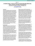
A summary of these three parts of the book is illustrated in Figure 1. It shows
three components: (A) DSP concepts, (B) embedded processor architecture and
real-time DSP considerations, and (C) real-life applications: a simple A-B-C
xiv
Preface
Part A: Digital Signal Processing Concepts
Chapter 2: Time-Domain Signals and Systems
Chapter 3: Frequency-Domain Analysis and
Processing
Chapter 4: Digital Filtering
Part B: Embedded Signal Processing Systems
and Concepts
Chapter 5: Introduction to the Blackfin
Processor
Chapter 6: Real-Time DSP Fundamentals
and Implementation Considerations
Chapter 7: Memory System and Data Transfer
Chapter 8: Code Optimization and Power
Management
Part C: Real-World Applications
Chapter 9: Audio Coding and Audio Effects
Chapter 10: Digital Image Processing
o This part may be skipped for
those who already familiar
with DSP. However, it serves
as a quick reference.
o It provides a good platform for
learning software tools.
o Part B integrates the
embedded processor’s
architecture, programming and
integrating hardware and
software into a complete
embedded system.
o It provides a good platform to
learn the in-depth details of
development tools.
o It contains many hands-on
examples and exercises in
using the Blackfin processors.
o Explore more advanced, realtime, and real-world
applications.
o Implement a working
prototype running on the
Blackfin EZ-KIT Lite
Figure 1 Summary of the book: contents and how to use them
approach to learning embedded signal processing with the micro signal
architecture.
DESCRIPTION OF EXAMPLES, EXERCISES,
EXPERIMENTS, PROBLEMS, AND
APPLICATION PROJECTS
This book provides readers many opportunities to understand and explore the main
contents of each chapter through examples, quizzes, exercises, hands-on experiments, exercise problems, and application projects. It also serves as a good hands-on
workbook to learn different embedded software tools (MATLAB, VisualDSP++,
and LabVIEW Embedded) and solve practical problems. These hands-on sections
are classified under different types as follows.
1. Examples provide a just-in-time understanding of the concepts learned in
the preceding sections. Examples contain working MATLAB problems to
illustrate the concepts and how problems can be solved. The naming convention for software example files is
Preface
xv
example{chapter number}_{example number}.m
They are normally found in the directory
c:\adsp\chap{x}\MATLAB_ex{x}\
where {x} is the chapter number.
2. Quizzes contain many short questions to challenge the readers for immediate feedback of understanding.
3. Experiments are mostly hands-on exercises to get familiar with the tools
and solve more in-depth problems. These experiments usually use MATLAB,
VisualDSP++, or LabVIEW Embedded. The naming convention for software
experiment files is
exp{chapter number}_{example number}
These experiment files can be found in the directory
c:\adsp\chap{x}\exp{x}_{no.}_<option>
where {no.} indicates the experiment number and <option> indicates the
BF533 or BF537 EZ-KIT.
4. Exercises further enhance the student’s learning of the topics in the preceding sections, examples, and experiments. They also provide the opportunity
to attempt more advanced problems to strengthen understanding.
5. Exercise Problems are located at the end of Chapters 1 to 8. These problem
sets explore or extend more interesting and challenging problems and
experiments.
6. Application Projects are provided at the end of Chapters 9 and 10 to serve
as mini-projects. Students can work together as a team to solve these
application-oriented projects and submit a report that indicates their
approaches, algorithms, and simulations, and how they verify the projects
with the Blackfin processor.
Most of the exercises and experiments require testing data. We provide two
directories that contain audio and image data files. These files are located in the
directories c:\adsp\audio_files and c:\adsp\image_files.
COMPANION WEBSITE
A website, www.ntu.edu.sg/home/ewsgan/esp_book.html, has been set up to support
the book. This website contains many supplementary materials and useful reference
links for each chapter. We also include a set of lecture slides with all the figures
and tables in PowerPoint format. This website will also introduce new hands-on
exercises and new design problems related to embedded signal processing. Because
the fast-changing world of embedded processors, the software tools and the Blackfin
xvi
Preface
processor will also undergo many changes as time evolves. The versions of software
tools used in this book are:
•
•
•
•
MATLAB Version 7.0
VisualDSP++ Version 4.0
LabVIEW 8.0
LabVIEW Embedded Edition 7.1
This website keeps track of the latest changes and new features of these tools. It
also reports on any compatibility problems when running existing experiments with
the newer version of software.
All the programs mentioned in the exercises and experiments are available
for download in the Wiley ftp site: ftp://ftp.wiley.com/public/sci_tech_med/
embedded_signal/.
We also include a feedback section to hear your comments and suggestions.
Alternatively, readers are encouraged to email us at [email protected] and
[email protected].
Learning Objective:
We learn by example and by direct experience because there are real limits to the
adequacy of verbal instruction.
Malcolm Gladwell, Blink: The Power of Thinking Without Thinking, 2005
Acknowledgments
We are very grateful to many individuals for their assistance in developing this
book. In particular, we are indebted to Todd Borkowski of Analog Devices,
who got us started in this book project. Without his constant support and encouragement, we would not have come this far. We would like to thank Erik B. Luther, Jim
Cahow, Mark R. Kaschner, and Matt Pollock of National Instruments for contributing to the experiments, examples, and writing in the LabVIEW Embedded
Module for Blackfin Processors. Without their strong commitment and support, we
would never have been able to complete many exciting demos within such a short
time. The first author would like to thank Chandran Nair and Siew-Hoon Lim of
National Instruments for providing their technical support and advice. We would
also like to thank David Katz and Dan Ledger of Analog Devices for providing
useful advice on Blackfin processors. Additionally, many thanks to Mike Eng, Dick
Sweeney, Tonny Jiang, Li Chuan, Mimi Pichey, and Dianwei Sun of Analog
Devices.
Several individuals at John Wiley also provided great help to make this book
a reality. We wish to thank George J. Telecki, Associate Publisher, for his support
of this book. Special thanks must go to Rachel Witmer, Editorial Program Coordinator, who promptly answered our questions. We would also like to thank Danielle
Lacourciere and Dean Gonzalez at Wiley for the final preparation of this book.
The authors would also like to thank Dahyanto Harliono, who contributed to
the majority of the Blackfin hands-on exercises in the entire book. Thanks also go
to Furi Karnapi, Wei-Chee Ku, Ee-Leng Tan, Cyril Tan, and Tany Wijaya, who
also contributed to some of the hands-on exercises and examples in the book. We
would also like to thank Say-Cheng Ong for his help in testing the LabVIEW
experiments.
This book is also dedicated to many of our past and present students who have
taken our DSP courses and have written M.S. theses and Ph.D. dissertations and
completed senior design projects under our guidance at both NTU and NIU. Both
institutions have provided us with a stimulating environment for research and teaching, and we appreciate the strong encouragement and support we have received.
Finally, we are greatly indebted to our parents and families for their understanding,
patience, and encouragement throughout this period.
Woon-Seng Gan and Sen M. Kuo
xvii
About the Authors
Woon-Seng Gan is an Associate Professor in the Information Engineering Division
in the School of Electrical and Electronic Engineering at the Nanyang Technological
University in Singapore. He is the co-author of the textbook Digital Signal Processors: Architectures, Implementations, and Applications (Prentice Hall 2005).
He has published more than 130 technical papers in peer-reviewed journals
and international conferences. His research interests are embedded media
processing, embedded systems, low-power-consumption algorithms, and real-time
implementations.
Sen M. Kuo is a Professor and Chair at the Department of Electrical Engineering,
Northern Illinois University, DeKalb, IL. In 1993, he was with Texas Instruments,
Houston, TX. He is the leading author of four books: Active Noise Control Systems
(Wiley, 1996), Real-Time Digital Signal Processing (Wiley, 2001, 2nd Ed. 2006),
Digital Signal Processors (Prentice Hall, 2005), and Design of Active Noise Control
Systems with the TMS320 Family (Texas Instruments, 1996). His research focuses
on real-time digital signal processing applications, active noise and vibration control,
adaptive echo and noise cancellation, digital audio applications, and digital
communications.
Note
• A number of illustrations appearing in this book are reproduced from copyright material published by Analog Devices, Inc., with permission of the
copyright owner.
• A number of illustrations and text appearing in this book are reprinted with
the permission of National Instruments Corp. from copyright material.
• VisualDSP++® is the registered trademark of Analog Devices, Inc.
• LabVIEWTM and National InstrumentsTM are trademarks and trade names of
National Instruments Corporation.
• MATLAB® is the registered trademark of The MathWorks, Inc.
• Thanks to the Hackles for providing audioclips from their singles “Leave It
Up to Me” copyright ©2006 www.TheHackles.com
xix
Chapter
1
Introduction
1.1 EMBEDDED PROCESSOR:
MICRO SIGNAL ARCHITECTURE
Embedded systems are usually part of larger and complex systems and are usually
implemented on dedicated hardware with associated software to form a computational engine that will efficiently perform a specific function. The dedicated hardware (or embedded processor) with the associated software is embedded into many
applications. Unlike general-purpose computers, which are designed to perform
many general tasks, an embedded system is a specialized computer system that is
usually integrated as part of a larger system. For example, a digital still camera takes
in an image, and the embedded processor inside the camera compresses the image
and stores it in the compact flash. In some medical instrument applications, the
embedded processor is programmed to record and process medical data such as
pulse rate and blood pressure and uses this information to control a patient support
system. In MP3 players, the embedded processor is used to process compressed
audio data and decodes them for audio playback. Embedded processors are also
used in many consumer appliances, including cell phones, personal digital assistants
(PDA), portable gaming devices, digital versatile disc (DVD) players, digital camcorders, fax machines, scanners, and many more.
Among these embedded signal processing-based devices and applications,
digital signal processing (DSP) is becoming a key component for handling signals
such as speech, audio, image, and video in real time. Therefore, many of the latest
hardware-processing units are equipped with embedded processors for real-time
signal processing.
The embedded processor must interface with some external hardware such as
memory, display, and input/output (I/O) devices such as coder/decoders to handle
real-life signals including speech, music, image, and video from the analog world.
It also has connections to a power supply (or battery) and interfacing chips for I/O
data transfer and communicates or exchanges information with other embedded
processors. A typical embedded system with some necessary supporting hardware
is shown in Figure 1.1. A single (or multiple) embedded processing core is used to
Embedded Signal Processing with the Micro Signal Architecture. By Woon-Seng Gan and
Sen M. Kuo
Copyright © 2007 John Wiley & Sons, Inc.
1
2
Chapter 1
Introduction
External
Memory
Analog-toDigital
Converter
Digital-toAnalog
Converter
Input/Output
Device
DMA
ROM/RAM/
Cache
I/O
Port
Embedded
Processing
Core
Power
Supply
Clock
System
Peripherals
Embedded Processor
Figure 1.1 Block diagram of a typical embedded system and its peripherals
perform control and signal processing functions. Hardware interfaces to the processing core include (1) internal memories such as read-only memory (ROM) for bootloading code and random-access memory (RAM) and cache for storing code and
data; (2) a direct memory access (DMA) controller that is commonly used to transfer
data in and out of the internal memory without the intervention of the main processing core; (3) system peripherals that contain timers, clocks, and power management
circuits for controlling the processor’s operating conditions; and (4) I/O ports that
allow the embedded core to monitor or control some external events and process
incoming media streams from external devices. These supporting hardware units
and the processing core are the typical building blocks that form an embedded
system. The embedded processor is connected to the real-world analog devices as
shown in Figure 1.1. In addition, the embedded processor can exchange data with
another system or processor by digital I/O channels. In this book, we use hands-on
experiments to illustrate how to program various blocks of the embedded system
and how to integrate them with the core embedded processor.
In most embedded systems, the embedded processor and its interfaces must
operate under real-time constraints, so that incoming signals are required to be
processed within a certain time interval. Failure to meet these real-time constraints
results in unacceptable outcomes like noisy response in audio and image applications, or even catastrophic consequences in some human-related applications like
automobiles, airplanes, and health-monitoring systems. In this book, the terms
“embedded processing” and “real-time processing” are often used interchangeably
to include both concepts. In general, an embedded system gathers data, processes
them, and makes a decision or responds in real time.
To further illustrate how different blocks are linked to the core embedded processor, we use the example of a portable audio player shown in Figure 1.2. In this
1.1 Embedded Processor: Micro Signal Architecture
3
BOOT FLASH
MEMORY
(FIRMWARE)
FLASH
MEMORY Ogg Vorbis STREAM
(COMPRESSED COMPRESSED AUDIO
AUDIO DATA)
ANALOG
DEVICES
®
DECODED AUDIO
OVER SERIAL PORT
AUDIO
DAC
AUDIO
OUTPUT
SDRAM
Figure 1.2 A block diagram of the audio media player (courtesy of Analog Devices, Inc.)
system, the compressed audio bit stream in Ogg Vorbis format (introduced in
Chapter 9) is stored in the flash memory external to the embedded processor, a
Blackfin processor. A decoding program for decoding the audio bit stream is loaded
from the boot flash memory into the processor’s memory. The compressed data are
streamed into the Blackfin processor, which decodes the compressed bit stream into
pulse code-modulated (PCM) data. The PCM data can in turn be enhanced by some
postprocessing tasks like equalization, reverberation, and three-dimensional audio
effects (presented in Chapter 9). The external audio digital-to-analog converter
(DAC) converts the PCM data into analog signal for playback with the headphones
or loudspeakers.
Using this audio media player as an example, we can identify several common
characteristics in typical embedded systems. They are summarized as follows:
1. Dedicated functions: An embedded system usually executes a specific task
repeatedly. In this example, the embedded processor performs the task of
decoding the Ogg Vorbis bit stream and sends the decoded audio samples
to the DAC for playback.
2. Tight constraints: There are many constraints in designing an embedded
system, such as cost, processing speed, size, and power consumption. In this
example, the digital media player must be low cost so that it is affordable to
most consumers, it must be small enough to fit into the pocket, and the
battery life must last for a long time.
3. Reactive and real-time performance: Many embedded systems must continuously react to changes of the system’s input. For example, in the digital
media player, the compressed data bit stream can be decoded in a number
of cycles per audio frame (or operating frequency for real-time processing).
In addition, the media player also must respond to the change of mode
selected by the users during playback.
4
Chapter 1
Introduction
Therefore, the selection of a suitable embedded processor plays an important
role in the embedded system design. A commonly used approach for realizing signal
processing tasks is to use fixed-function and hardwired processors. These are implemented as application-specific integrated circuits (ASICs) with DSP capabilities.
However, these hardwired processors are very expensive to design and produce, as
the development costs become significant for new process lithography. In addition,
proliferation and rapid change of new standards for telecommunication, audio,
image, and video coding applications makes the hardwired approach no longer the
best option.
An alternative is to use programmable processors. This type of processor allows
users to write software for the specific applications. The software programming
approach has the flexibility of writing different algorithms for different products
using the same processor and upgrading the code to meet emerging standards in
existing products. Therefore, a product can be pushed to the market in a shorter time
frame, and this significantly reduces the development cost compared to the hardwired approach. A programmable digital signal processor is commonly used in
many embedded applications. DSP architecture has evolved greatly over the last two
decades to include many advanced features like higher clock speed, multiple multipliers and arithmetic units, incorporation of coprocessors for control and communication tasks, and advanced memory configuration. The complexity of today’s
signal processing applications and the need to upgrade often make a programmable
embedded processor a very attractive option. In fact, we are witnessing a market
shift toward software-based microarchitectures for many embedded media processing applications.
One of the latest classes of programmable embedded signal processors is the
micro signal architecture (MSA). The MSA core [43] was jointly developed by Intel
and Analog Devices Inc. (ADI) to meet the computational demands and power constraints of today’s embedded audio, video, and communication applications. The
MSA incorporates both DSP and microcontroller functionalities in a single core.
Both Intel and ADI have further developed processors based on the MSA architecture
for different applications. The MSA core combines a highly efficient computational
architecture with features usually only available on microcontrollers. These features
include optimizations for high-level language programming, memory protection, and
byte addressing. Therefore, the MSA has the ability to execute highly complex DSP
algorithms and basic control tasks in a single core. This combination avoids the need
for a separate DSP processor and microcontroller and thus greatly simplifies both
hardware and software design and implementation. In addition, the MSA has a very
efficient and dynamic power management feature that is ideal for a variety of batterypowered communication and consumer applications that require high-intensity signal
processing on a strict power budget. In fact, the MSA-based processor is a versatile
platform for processing video, image, audio, voice, and data.
Inside the computational block of the MSA, there are two multiply-add units,
two arithmetic-logic units, and a single shifter. These hardware engines allow the
MSA-based processor to efficiently perform several multiply-add operations in
1.1 Embedded Processor: Micro Signal Architecture
5
parallel to support complex number crunching tasks. The availability of these hardware units coupled with high clock speed (starts from 300 MHz and rises steadily
to the 1-GHz range) has created a substantial speed improvement over conventional
microprocessors. The detailed architecture of the MSA core is explained with simple
instructions and hands-on experiments in Chapter 5.
The MSA core uses a simple, reduce-instruction-set-computer (RISC)-like
instruction set for both control and signal processing applications. The MSA also
comes with a set of multifunction instructions that allows different sizes of op-codes
to be combined into a single instruction. Therefore, the programmer has the flexibility of reducing the code size, and at the same time, maximizing the usage of available resources. In addition, some special instructions support video and wireless
applications. This chapter introduces some basic features of programming and
debugging the MSA core and uses examples and exercises to highlight the important
features in the software tools. In subsequent chapters, we introduce more advanced
features of the software tools.
The MSA core is a fixed-point processor. It operates on fixed-point fractional
or integer numbers. In contrast to the floating-point processors, such as the Intel
Pentium processors, fixed-point processors require special attention to manipulating
numbers to avoid wrong results or extensive computation errors. The concepts of
real-time implementation using a fixed-point processor are introduced and examined
in Chapter 6.
As explained above, the embedded core must be combined with internal and
external memories, serial ports, mixed signal circuits, external memory interfaces,
and other peripherals and devices to form an embedded system. Chapter 7 illustrates
how to program and configure some of these peripherals to work with the core processor. Chapter 8 explains and demonstrates several important techniques of optimizing the program written for the MSA core. This chapter also illustrates a unique
feature of the MSA core to control the clock frequency and supply voltage to the
MSA core via software, so as to reduce the power consumption of the core during
active operation.
In this book, we examine the MSA core with the latest Blackfin processors
(BF5xx series) from ADI. The first generation of Blackfin processors is the BF535
processor, which operates at 300 MHz and comes with L1 and L2 cache memories,
system control blocks, basic peripheral blocks, and high-speed I/O. The next generation of Blackfin processors consists of BF531, BF532, BF533, and BF561 processors.
These processors operate at a higher clock speed of up to 750 MHz and contain
additional blocks like parallel peripheral interface, voltage regulator, external
memory interface, and more data and instruction cache. The BF531 and BF532 are
the least expensive and operate at 400 MHz, and the BF561 is a dual-core Blackfin
processor that is targeted for very high-end applications. The BF533 processor operates at 750 MHz and provides a good platform for media processing applications.
Recently released Blackfin processors include BF534, BF536, and BF537. These
processors operate at around 400–500 MHz and feature a strong support for Ethernet
connection and a wider range of peripherals.
6
Chapter 1
Introduction
Because all Blackfin processors are code compatible, the programs written for
one processor can be easily ported to other processors. This book uses BF533 and
BF537 processors to explain architecture, programming, peripheral interface, and
implementation issues. The main differences between the BF533 and the BF537 are
the additional peripheral supports and slightly less internal instruction memory of
the BF537 processors. Therefore, explanation of the Blackfin processing core can
be focused solely on the BF533, and additional sections are introduced for the extra
peripheral supports in the BF537.
There are several low-cost development tools introduced by ADI. In this book,
we use the VisualDSP++ simulator to verify the correctness of the algorithm and
the EZ-KIT (development board that contains the MSA processor, memory, and
other peripherals) for the Blackfin BF533 and BF537 processors for real-time signal
processing and control applications. In addition, we also use a new tool (LabVIEW
Embedded Module for Blackfin Processors) jointly developed by National Instruments (NI) and ADI to examine a new approach in programming the Blackfin processor with a blockset programming approach.
1.2
REAL-TIME EMBEDDED SIGNAL PROCESSING
DSP plays an important role in many real-time embedded systems. A real-time
embedded system is a system that requires response to external inputs within a
specific period. For example, a speech-recognition device sampling speech at 8 kHz
(bandwidth of 4 kHz) must respond to the sampled signal within a period of 125 μs.
Therefore, it is very important that we take special attention to define the real-time
system and highlight some special design considerations that apply to real-time
embedded signal processing systems.
Generally, a real-time system must maintain a timely response to both internal
and external signal/data. There are two types of real-time system: hard and soft
real-time systems. For the hard real-time system, an absolute deadline for the completion of the overall task is imposed. If the hard deadline is not met, the task has
failed. For example, in the case of speech enhancement, the DSP software must be
completed within 125 μs; otherwise, the device will fail to function correctly. In the
case of a soft real-time system, the task can be completed in a more relaxed time
range. For example, it is not critical how long it takes to complete a credit card
transaction. There is no hard deadline by which the transaction must be completed,
as long as it is within a reasonable period of time.
In this book, we only examine hard real-time systems because all embedded
media processing systems are hard real-time systems. There are many important
challenges when designing a hard real-time system. Some of the challenges
include:
1. Understanding DSP concepts and algorithms. A solid understanding of
the important DSP principles and algorithms is the key to building a successful real-time system. With this knowledge, designers can program and
optimize the algorithm on the processor using the best parameters and set-
1.3 Introduction to the Integrated Development Environment VisualDSP++
2.
3.
4.
5.
7
tings. Chapters 2 to 4 introduce the fundamentals of DSP and provide many
hands-on experiments to implement signal processing algorithms.
Resource availability. The selection of processor core, peripherals, sensors
and actuators, user interface, memory, development, and debugging tools is
a complex task. There are many critical considerations that make the decision tough. Chapter 5 shows the architecture of the Blackfin processor and
highlights its strength in developing the embedded system.
Arithmetic precision. In most embedded systems, a fixed-point arithmetic
is commonly used because fixed-point processors are cheaper, consume less
power, and have higher processing speed as compared to floating-point processors. However, fixed-point processors are more difficult to program and
also introduce many design challenges that are discussed in Chapter 6.
Response time requirements. Designers must consider hardware and software issues. Hardware considerations include processor speed, memory size
and its transfer rate, and I/O bandwidth. Software issues include programming language, software techniques, and programming the processor’s
resources. A good tool can greatly speed up the process of developing and
debugging the software and ensure that real-time processing can be achieved.
Chapter 7 explains the peripherals and I/O transfer mechanism of the Blackfin processor, whereas Chapter 8 describes the techniques used in optimizing
the code in C and assembly programming.
Integration of software and hardware in embedded system. A final part of
this book implements several algorithms for audio and image applications.
The Blackfin BF533/BF537 EZ-KITs are used as the platform for integration
of software and hardware.
To start the design of the embedded system, we can go through a series of
exercises using the development tools. As we progress to subsequent chapters, more
design and debugging tools and features of these tools are introduced. This progressive style in learning the tools will not overload the users at the beginning. We use
only the right tool with just enough features to solve a given problem.
1.3 INTRODUCTION TO THE INTEGRATED
DEVELOPMENT ENVIRONMENT VISUALDSP+ +
In this section, we examine the software development tool for embedded signal
processors. The software tool for the Blackfin processor is the VisualDSP++ [33]
supplied by ADI. VisualDSP++ is an integrated development and debugging
environment (IDDE) that provides complete graphical control of the edit, build,
and debug processes. In this section, we show the detailed steps of loading a
project file into the IDDE, building it, and downloading the executable file into
the simulator (or the EZ-KIT). We introduce some important features of the
VisualDSP++ in this chapter, and more advanced features are introduced in subsequent chapters.
8
Chapter 1
1.3.1
Introduction
Setting Up VisualDSP+ +
The Blackfin version of VisualDSP++ IDDE can be downloaded and tested for a
period of 90 days from the ADI website. Once it is downloaded and installed, a
VisualDSP+ + Environment icon
will appear on the desktop. Double-click
on this icon to activate the VisualDSP++. A New Session window will appear as
shown in Figure 1.3. Select the Debug target, Platform, and Processor as shown in
Figure 1.3, and click OK to start the VisualDSP++. Under the Debug target option,
there are two types of Blackfin simulator, a cycle-accurate interpreted simulator and
a functional compiled simulator. When ADSP_BF5xx Blackfin Family Simulators
is selected, the cycle-accurate simulator is used. This simulator provides a more
accurate performance, and thus is usually used in this book. The compiled simulator
is used when the simulator needs to process a large data file. The Processor option
allows users to select the type of processor. In this book, only the Blackfin BF533 and
BF537 processors are covered. However, the code developed for any Blackfin processor is compatible with other Blackfin processors. In Figure 1.3, the ADSP-BF533
simulator is selected. Alternatively, users can select the ADSP-BF537 simulator.
A VisualDSP++ Version 4 window is shown in Figure 1.4. There are three
subwindows and one toolbar menu in the VisualDSP++ window. A Project Window
displays the files available in the project or project group. The Disassembly window
displays the assembly code of the program after the project has been built. The
Output Window consists of two pages, Console and Build. The Console page
displays any message that is being programmed in the code, and the Build page
shows any errors encountered during the build process. The toolbar menu contains
all the tools, options, and modes available in the VisualDSP++ environment. We
will illustrate these tools as we go through the hands-on examples and exercises in
Figure 1.3 A New Session window
1.3 Introduction to the Integrated Development Environment VisualDSP++
9
Toolbar
menu
Figure 1.4 VisualDSP++ window
this and following chapters. Click on Project Æ Project Options and make sure
that the right processor is selected for the targeted simulator.
1.3.2 Using a Simple Program
to Illustrate the Basic Tools
In this section, we illustrate the basic tools and features in the VisualDSP++ IDDE
through a series of simple exercises. We use a sample project that consists of two
source files written in C for the Blackfin processor.
HANDS-ON EXPERIMENT 1.1
In this experiment, we first start the VisualDSP++ environment as explained above. Next,
click on the File menu in the toolbar menu and select Open Æ Project. . . . Look for the
project file exp1_1.dpj under directory c:\adsp\chap1\exp1_1 and double-click on
the project file. Once the project file is loaded into the VisualDSP++ environment, we can
see a list of source files. Double-click on dotprod_main.c to see the source code in the
editor window (right side) as shown in Figure 1.5.
Scroll through the source code in both dotprod_main.c and dotprod.c. This is a
simple program to perform multiply-accumulate (or dot product) of two vectors, a and b.
From the Settings menu, choose Preferences to open the dialog box as shown in Figure 1.6.
10
Chapter 1
Introduction
Figure 1.5 Snapshot of the C file dotprod_main.c displayed in the source window
Figure 1.6 Preferences dialog box
Under the General preference, click on Run to main after load and Load executable after
build. The first option starts executing from the void main() of the program after the
program is loaded into the simulator. The second option enables the code to be loaded into
the processor memory after the code is being built. The rest of the options can be left as
default. Click OK to close the Preferences dialog box.
Now, we are ready to build the project. We can either click on Project Æ Build
Project in the toolbar menu or press the function key F7. There is a build icon
that
1.3 Introduction to the Integrated Development Environment VisualDSP++
11
can be used to perform the build operation. The build operation basically combines the
compile, assembler, and link processes to obtain an executable file (.dxe). Users will find
the executable file exp1_1.dxe being created in directory c:\adsp\chap1\exp1_1\
debug after the build operation. Besides the Build Project option, there is the Rebuild
icon). The Rebuild All option builds the project regardless of whether
All option (or
the project build is up to date. The message Build completed successfully is
shown in the Build page of the Output Window if the build process detects no error.
However, users will notice that the build process detects an undefined identifier, as shown
in Figure 1.7.
Users can double-click on the error message (in red), and the cursor will be placed on
the line that contains the error. Correct the typo by changing results to result and save
the source file by clicking on File Æ Save Æ File dotprod_main.c. The project is now built
without any error, as indicated in the Output window.
Once the project has been built, the executable file exp1_1.dxe is automatically
downloaded into the target (enabled in the Preferences dialog box), which is the BF533 (or
BF537) simulator. Click on the Console page of the Output Window. A message appears
stating that the executable file has been completely loaded into the target, and there is a
Breakpoint Hit at <ffa006f8>. A solid red circle (indicates breakpoint) and a yellow
arrow (indicates the current location of the program pointer) are positioned at the left-hand
edges of the source code and disassembly code, as shown in Figure 1.8.
The VisualDSP++ automatically sets two breakpoints, one at the beginning and the
other at the end of the code. The location of the breakpoint can be viewed by clicking on
Setting Æ Breakpoints as shown in Figure 1.9. Users can click on the breakpoint under
the Breakpoint list and click the View button to find the location of the breakpoint in the
Figure 1.7 Error message appears after building the project
Editor window
Disassembly
window
Red circle and yellow arrow
Figure 1.8 Breakpoint displayed in both editor and disassembly windows
12
Chapter 1
Introduction
Figure 1.9 Breakpoint dialog box
Disassembly window. The breakpoint can be set or cleared by double-clicking on the gray
gutter (Fig. 1.8) next to the target code in the editor and disassembly window.
The project is now ready to run. Click on the run button
or Debug Æ Run (F5).
The simulator computes the dot product (sum of products or multiply-accumulate) and displays the result in the Console page of the Output Window. What is the answer for the dot
product between arrays a and b?
Modify the source files to perform the following tasks:
1. Add a new 20-element array c; perform the dot product computation between arrays
a and c and display the result.
2. Recompute the dot product of the first 10 elements in the arrays.
3. To obtain the cycle count of running the code from start to finish, we can use the
cycle registers. Simply click on Register Æ Core Æ Cycles. Reload the program by
clicking on File Æ Reload Program. The program pointer will reset to the beginning of the program. In the Cycle window, clear the CYCLE register value to 0 to
initialize the cycle counter. Run the program and note the cycle count. Note: To
display the cycle count in unsigned integer format, right-click on the Cycle window
and select unsigned integer.
1.3.3 Advanced Setup: Using the
Blackfin BF533 or BF537 EZ-KIT
In the previous hands-on experiments, we ran the program with the BF533 (or
BF537) simulator. In this section, we perform the same experiment with the Blackfin
1.3 Introduction to the Integrated Development Environment VisualDSP++
Audio
input
Audio
output
Power
in
13
Video
I/O
SW9
123456
on
off
BF533
processor
SDRAM
USB
interface
General-purpose
LEDs
General-purpose
push buttons
SW4 SW5 SW6 SW7
Figure 1.10 The BF533 EZ-KIT
BF533 (or BF537) EZ-KIT. The EZ-KIT board is a low-cost hardware platform that
includes a Blackfin processor surrounded by other devices such as audio coder/
decoder (CODEC), video encoders, video decoders, flash, synchronous dynamic
RAM (SDRAM), and so on. We briefly introduce the hardware components in the
EZ-KIT and show the differences between the BF533 and BF537 boards.
Figure 1.10 shows a picture of the BF533 EZ-KIT [29]. This board has four
audio input and six audio output channels via the RCA jacks. In addition, it can
also encode and decode three video inputs and three video outputs. Users can
also program the four general-purpose push buttons (SW4, SW5, SW6, and
SW7) and six general-purpose LEDs (LED4–LED9). The EZ-KIT board is interfaced with the VisualDSP++ (hosted on personal computer) via the USB interface
cable.
Figure 1.11 shows a picture of the BF537 EZ-KIT [30]. This board consists of
stereo input and output jack connectors. However, the BF537 EZ-KIT does not have
any video I/O. Instead, it includes the IEEE 802.3 10/100 Ethernet media access
control and controller area network (CAN) 2.0B controller. Similar to the BF533
EZ-KIT, the BF537 EZ-KIT has four general-purpose push buttons (SW10, SW11,
SW12, and SW13) and six general-purpose LEDs (LED1–LED6). Other feature
differences between BF533 and BF537 EZ-KITs are highlighted in subsequent
chapters.
14
Chapter 1
Introduction
Ethernet
MAC
Power
in
USB
interface
SW10
SW11
SW12
SW13
General-purpose
LEDs
BF537
processor
General-purpose
push buttons
CAN
Figure 1.11 The BF537 EZ-KIT
This section describes the setup of the BF533 EZ-KIT [31]. The EZ-KIT’s
power connector is first connected to the power supply. Turn on the power supply
and verify that the green LED is lit and LEDs 4–9 continue to roll (indicating that
the board is not linked to the software). Next, the USB cable is connected from the
computer to the EZ-KIT board. The window environment recognizes the new hardware and launches the Add New Hardware Wizard, which installs files located on
the EZ-KIT CD-ROM. Once the USB driver is installed successfully, the yellow
LED (USB monitor) should remain lit. A similar setup can also be carried out for
the BF537 EZ-KIT [32]. Users can refer to the BF533 (or BF537) EZ-KIT Evaluation System Manual for more details on the settings.
The VisualDSP++ environment can be switched to the EZ-KIT target by the
following steps. Click on Session Æ New Session. A New Session window will
appear. Change the debug target and platform to that shown in Figure 1.12 (setup
for the BF533 EZ-KIT). Click OK and note the change in the title bar of the
VisualDSP++. We are now ready to run the same project on the BF533 EZ-KIT.
Similarly, if the BF537 EZ-KIT is used, select the desired processor and its
EZ-KIT.
Build the project and run the executable file on the EZ-KIT, using the same
procedure as before. Do you notice any difference in the building process on the
EZ-KIT platform compared to the simulator? Next, obtain the cycle count in running
the same program on the EZ-KIT. Is there any change in the cycle count as compared to the simulator?
1.4 More Hands-on Experiments
15
Figure 1.12 New Session window setup for BF533 EZ-KIT
1.4
MORE HANDS-ON EXPERIMENTS
We have learned how to load a project file into the Blackfin simulator and EZ-KIT.
In this section, we create a new project file from scratch and use the graphic features
in the VisualDSP++ environment. The following experiments apply to both BF533
and BF537 EZ-KITs.
HANDS-ON EXPERIMENT 1.2
1. Using the previous source files as templates, create two new source files
vecadd_main.c and vecadd.c to perform vector addition of two arrays a
and b. The result is saved in the third array c. Use File Æ New Æ File to
create a blank page for editing in the VisualDSP++. Save these files in directory
c:\adsp\chap1\exp1_2.
2. From the File menu, choose New and then Project to open the Project Wizard.
Enter the directory and the name of the new project as shown in Figure 1.13. Click
on Finish and Yes to create a new project.
3. An empty project is created in the Project window. Click on Project Æ Project
Options to display the Project Options dialog box as shown in Figure 1.14. The
default settings are used, and the project creates an executable file (.dxe). Because
Settings for configuration is set to Debug, the executable file also contains debug
information for debugging.
4. Click on Compile Æ General (1), and click on Enable optimization to enable the
optimization for speed as shown in Figure 1.15. Click OK to apply changes to the
project options.
5. To add the source files to the new project, click on Project Æ Add to Project Æ
File(s). . . . Select the two source files and click Add. The sources files are now
added to the project file.
16
Chapter 1
Introduction
Figure 1.13 Project Wizard window
Figure 1.14 Project Options dialog box
1.4 More Hands-On Experiments
17
Figure 1.15 Project wizard option for compile
Figure 1.16 Plot Configuration dialog box
6. Build the project by following the steps given in Hands-On Experiment 1.1. Run the
project and verify that the correct result in array c is displayed in the Output
Window.
HANDS-ON EXPERIMENT 1.3
1. In this hands-on experiment, we introduce some useful graphic features in the
VisualDSP++ environment. We plot the three arrays, a, b, and c, used in the previous experiment.
2. Make sure that the project is built and loaded into the simulator. Click on View Æ
Debug Windows Æ Plot Æ New. A Plot Configuration dialog box appears as
shown in Figure 1.16. We type in a and 20 and select int in Address, Count, and
18
Chapter 1
Introduction
Array a
Values
5,000
0
0
2
4
6
8
10
12
14
16
18
20
22
Number of elements
Figure 1.17 Display of array a
Data boxes, respectively. Click on Add to add in the array a. Use similar steps to
plot the other two arrays. Modify the plot settings to make a graph as displayed in
Figure 1.17.
3. Finally, add in the other two arrays in the same plot or create two new plots.
So far, we have learned how to program in C and run the code with the Blackfin
simulator and EZ-KITs. In the following section, we introduce a new graphical
development environment, LabVIEW Embedded Module for Blackfin Processors,
jointly developed by NI and ADI. This new tool provides an efficient approach to
prototyping embedded signal processing systems. This new rapid prototyping tool
uses a graphical user interface (GUI) to control and select parameters of the signal
processing algorithms and view updates of graphical plots on the fly.
1.5 SYSTEM-LEVEL DESIGN USING A
GRAPHICAL DEVELOPMENT ENVIRONMENT
Graphical development environments, such as National Instruments LabVIEW,
are effective means to rapidly prototype and deploy developments from individual algorithms to full system-level designs onto embedded processors. The graphical data flow paradigm that is used to create LabVIEW programs or virtual
instruments (VIs) allows for rapid, intuitive development of embedded code. This
is due to its flowchart-like syntax and inherent ease in implementing parallel
tasks.
In this section and sections included at the end of each subsequent chapter, we
present a common design cycle that engineers are using to reduce product development time by effectively integrating the software tools they use on the desktop for
deployment and testing. This will primarily be done with the LabVIEW Embedded
1.5 System-Level Design Using a Graphical Development Environment
19
Development Module for the ADI Blackfin BF533 and BF537 processors which is
an add-on module for LabVIEW to target and deploy to the Blackfin processor.
Other LabVIEW add-ons, such as the Digital Filter Design Toolkit, may also be
discussed.
Embedded system developers frequently use computer simulation and design
tools such as LabVIEW and the Digital Filter Design Toolkit to quickly develop a
system or algorithm for the needs of their project. Next, the developer can leverage
his/her simulated work on the desktop by rapidly deploying that same design with
the LabVIEW Embedded Module for Blackfin Processors and continue to iterate on
that design until the design meets the design specifications. Once the design has
been completed, many developers will then recode the design using VisualDSP++
for the most efficient implementation. Therefore, knowledge of the processor architecture and its C/assembly programming is still important for a successful implementation. This book provides balanced coverage of both high-level programming
using the graphical development environment and conventional C/assembly programming using VisualDSP++.
In the first example using this graphical design cycle, we demonstrate the
implementation and deployment of the dot product algorithm presented in Hands-On
Experiment 1.1 using LabVIEW and the LabVIEW Embedded Module for Blackfin
Processors.
1.5.1 Setting up LabVIEW and LabVIEW
Embedded Module for Blackfin Processors
LabVIEW and the LabVIEW Embedded Module for Blackfin Processors (trial
version) can be downloaded from the book companion website. A brief tutorial on
using these software tools is included in Appendix A of this book. Once they are
installed, double-click on National Instruments LabVIEW 7.1 Embedded Edition
under the All Programs panel of the start menu. Hands-On Experiment 1.4 provides
an introduction to the LabVIEW Embedded Module for Blackfin Processors to
explore concepts from the previous hands-on experiments.
HANDS-ON EXPERIMENT 1.4
This exercise introduces the NI LabVIEW Embedded Module for Blackfin Processors and
the process for deploying graphical code on the Blackfin processor for rapid prototyping and
verification. The dot product application was created with the same vector values used previously in the VisualDSP++ project file, exp1_1.dpj. This experiment uses arrays, functions, and the Inline C Node within LabVIEW.
From the LabVIEW Embedded Project Manager window, open the project file
DotProd – BF5xx.lep located in directory c:\adsp\chap1\exp1_4. Next, doubleclick on DotProd_BF.vi from within the project window to open the front panel. The front
panel is the graphical user interface (GUI), which contains the inputs and outputs of the
20
Chapter 1
Introduction
Figure 1.18 Front panel of DotProd.vi
Figure 1.19 Block diagram of DotProd.vi
program as shown in Figure 1.18. Select View Æ Block Diagram to switch to the LabVIEW
block diagram, shown in Figure 1.19, which contains the source code of the program. The
dot product is implemented by passing two vectors (or one-dimensional arrays) to the Dot
Product function. The result is then displayed in the Dot Product Result indicator. The
value is also passed to the standard output buffer, because controls and indicators are only
available in JTAG debug or instrumented debug modes. The graphical LabVIEW code
executes based on the principle of data flow, in this case from left to right.
This graphical approach to programming makes this program simple to implement and
self-documenting, which is especially helpful for larger-scale applications. Also note the use
of the Inline C Node, which allows users to test existing C code within the graphical framework of LabVIEW.
Now run the program by clicking on the Run arrow
to calculate the dot product
of the two vectors. The application will be translated, linked, compiled, and deployed to the
Blackfin processor. Open the Processor Status window and select Output to see the numeric
result of the dot product operation.
Another feature available for use with the LabVIEW Embedded Module for Blackfin
Processors is instrumented debug mode, which allows users to probe wires on the LabVIEW
block diagram and interact with live-updating front panel controls and indicators while the
code is actually running on the Blackfin. Instrumented debug can be accomplished through
TCP (Ethernet) on the BF537 and through JTAG (USB) on both the BF537 and BF533 processors. To use instrumented debug, run the application in debug mode, using the Debug
button
. Try changing vector elements on the front panel and probing wires on the block
diagram. For additional configuration, setup, and debugging information, refer to Getting
Started with the LabVIEW Embedded Module for Analog Devices Blackfin Processors [52],
found in the book companion website.
1.6 More Exercise Problems
1.6
21
MORE EXERCISE PROBLEMS
1. List 10 embedded systems in Table 1.1 that are required to perform some forms of DSP.
Explain the signal processing tasks.
2. Survey the key components in a typical iPod player.
3. Survey the key components in a typical digital camera.
4. Survey the differences between fixed-function processors and programmable processors.
State the advantages and disadvantages of these processors.
5. In Hands-on Experiment 1.1, C language is used to program the Blackfin processor. A
low-level assembly program can also be used to compute the dot product. The low-level
assembly code uses a standard set of assembly syntaxes. These assembly syntaxes are
introduced in Chapter 5 onward. Use the Blackfin simulator (either BF533 or BF537) to
create a new project file that includes the source codes available in directory c:\adsp\
chap1\problem1_5. Examine the source files and understand the differences between
the C function code in Experiment 1.1 and the assembly function code listed in this
exercise. Benchmark and compare the cycle count for performing the same dot product
with assembly code with that obtained with C code. Also benchmark the C code with
optimization enabled.
6. Implement the same project in the Blackfin (either BF533 or BF537) EZ-KIT. Any difference in the cycle counts compared to the Blackfin simulator?
Table 1.1
DSP Tasks in Embedded Systems
Embedded Systems
(1)
(2)
(3)
(4)
(5)
(6)
(7)
(8)
(9)
(10)
DSP Tasks
22
Chapter 1
Introduction
7. The Fibonacci series can be computed by adding the two successive numbers to form the
next number in the series. Generate the Fibonacci series for the fi rst 10 numbers of 1, 1,
2, 3, 5, 8, 13, 21, 34, 55 . . . , using the Blackfin simulator, starting from the first two
numbers. Verify your answer in the Blackfin memory window.
8. Refer to the ADI manual on getting started with VisualDSP++ [34] and go through
all the experiments described in the manual. The manual can be found in the ADI
website.
Part A
Digital Signal
Processing Concepts
Chapter
2
Time-Domain Signals
and Systems
T
his chapter uses several noise reduction examples and experiments to introduce
important time-domain techniques for processing digital signals and analyzing
simple DSP systems. The detailed analysis and more advanced methods are introduced in Chapter 3, using frequency-domain techniques.
2.1
INTRODUCTION
With the easy accessibility of increasingly powerful personal computers and the
availability of powerful and easy-to-use MATLAB [48] software for computer
simulations, we can now learn DSP concepts more effectively. This chapter uses
hands-on methods to introduce fundamental time-domain DSP concepts because
it is more interesting to examine real-world DSP applications with the help of
interactive MATLAB tools.
In particular, this chapter uses the latest powerful graphical user interface
(GUI) tool called Signal Processing Tool, which comes with the Signal Processing
Toolbox [49]. Because each experiment requires a set of general problem-solving
skills and related DSP principles, we provide multiple contexts including the necessary
DSP theory, computer simulations, and hands-on experiments for achieving thorough
understanding. Most of the DSP subjects are covered in the introduction to hands-on
exercises and experiments. These experiments are organized to introduce DSP
subjects from the simple introductory subjects in this chapter and gradually introduce
more complicated experiments and applications in subsequent chapters. Each
experiment introduces and applies just enough information at that time to complete
the required tasks. This is similar to using a “spiral learning” technique to continually
circle back and cover concepts in more and more depth throughout Chapters 2, 3,
and 4.
Embedded Signal Processing with the Micro Signal Architecture. By Woon-Seng Gan and
Sen M. Kuo
Copyright © 2007 John Wiley & Sons, Inc.
25
26
Chapter 2 Time-Domain Signals and Systems
Projects introduced in this chapter are based on designing simple filters to
remove broadband (white) noise that corrupts the desired narrowband (sinusoidal)
signal. First, a MATLAB example shows how to generate a digital signal and use
it to introduce a sampling theorem. A quiz is provided immediately afterward to
ensure that we understand the relationship between analog and digital worlds. A
hands-on experiment implements the moving-average filter with length L = 5, 10,
and 20, using the MATLAB code. We find that when the filter is working for L =
5, it reduces more noise when L = 10 with higher undesired signal attenuation, but
are surprised to learn that the filter output approaches zero when L = 20. Finally,
for more complicated problems of adding different noises (sinusoidal and white) to
the speech, we have to enhance the desired speech. We use the simple movingaverage filter but fail. Now our interest is piqued to learn more advanced DSP
techniques in Chapters 3 and 4. In this fashion, we learn important DSP concepts
repeatedly at each project by doing hands-on experiments and exercises. We continually circle back the DSP subjects and cover concepts in more and more depth
throughout the book.
2.2
TIME-DOMAIN DIGITAL SIGNALS
A digital signal x(n) is defined as a function of time index n, which corresponds to
time at nTs seconds if the signal is sampled from an analog signal x(t) with the
sampling period Ts seconds. The sampling period can be expressed as
Ts =
1
,
fs
(2.2.1)
where fs is the sampling frequency (or sampling rate) in hertz (or cycles per second).
For many real-world applications, the required sampling rates are defined by the
given applications. For example, the sampling rate for telecommunications is
8,000 Hz (or 8 kHz), and for compact discs (CDs) it is 44.1 kHz.
2.2.1
Sinusoidal Signals
An analog sine wave can be expressed as
x (t ) = A sin (2πft ) = A sin (Ωt ) ,
(2.2.2)
where A is the amplitude, f is the frequency of the sine wave in hertz, and Ω = 2πf
is the frequency in radians per second. If we sample this analog sine wave with
sampling rate fs, we obtain a digital sine wave x(n) with samples at time 0, Ts,
2Ts, . . . nTs, . . . . This digital signal can be expressed by replacing t with nTs in
Equation 2.2.2 as
x ( n ) ≡ x ( nTs ) = A sin (2πfnTs ) = A sin (ωn ) ,
(2.2.3)
where the digital frequency ω in radians per sample (or simply radians) is
defined as
2.2 Time-Domain Digital Signals
ω = 2 πf Ts = 2 πf fs , − π ≤ ω ≤ π.
27
(2.2.4)
It is important to note that the sampling rate must satisfy the Nyquist sampling
theorem expressed as
fs ≥ 2 fN ,
(2.2.5)
where f N is the maximum frequency component (or bandwidth) of the signal, which
is also called a Nyquist frequency. If fs < 2f N, frequency components higher than
fs /2 will fold back to the frequency range from 0 Hz to fs /2 Hz, which results in a
distortion called aliasing. The sampling theorem implies that digital signals can only
have meaningful representation of signal components from 0 Hz to fs /2 Hz.
EXAMPLE 2.1
We can generate a 200-Hz sine wave that is sampled at 4,000 Hz (or 4 kHz) using the
MATLAB program example2_1.m. A partial code is listed as follows:
fs = 4000;
%
f = 200;
%
n = 0:1:fs/f;
%
xn = sin(2*pi*f*n/fs); %
plot(n,xn,’-o’);grid on;
sampling rate is 4 kHz
frequency of sinewave is 200 Hz
time index n that cover one cycle
generate sinewave
The generated sine wave is shown in Figure 2.1, in which the digital samples are marked by
open circles. Digital signal x(n) consists of those discrete-time samples; however, we usually
200 Hz sine wave sampled at 4,000 Hz
1
0.8
0.6
x(t), analog waveform
x(2Ts)
Amplitude A
0.4
0.2
sampling period, Ts
x(Ts)
0
–0.2
x(0)
–0.4
–0.6
–0.8
–1
0
2
4
6
8
12
10
Time index nTs
14
16
18
20
Figure 2.1 One cycle of 200-Hz sine wave sampled at 4,000 Hz. Signal samples are marked by
open circles
28
Chapter 2 Time-Domain Signals and Systems
plot a digital signal by connecting those samples with a line such as x(t) shown in
Figure 2.1.
Based on Equation 2.2.1, the sampling period Ts = 1/4,000 s. As shown in Figure 2.1,
one cycle of sine wave consists of 20 samples. Therefore, the period of sine wave is
(1/4,000) × 20 = 1/200 s, which is equivalent to the frequency of 200 Hz.
QUIZ 2.1
1. If the sine wave shown in Figure 2.1 is obtained by sampling an analog sine
wave with a sampling rate of 100 Hz, what is the frequency of the sine wave?
Why?
2. If the frequency of the sine wave shown in Figure 2.1 is 20 Hz, what is the
sampling period used for obtaining these digital samples? Why?
3. If we want to produce 3 s of analog sine wave by converting a digital sine
wave with a digital-to-analog (D/A) converter (DAC) with a sampling rate
of 4 kHz, how many digital samples are needed?
Quiz 2.1 shows that the frequency of a digital signal is dependent on the sampling rate fs. Therefore, it is more convenient to use the normalized digital frequency
defined as
F ≡ f ( fs 2 ) , − 1 ≤ F ≤ 1
(2.2.6)
with unit cycles per sample. Comparing this definition with Equation 2.2.4, we show
that ω = Fπ. For example, the digital frequency of the sine wave shown in Figure
2.1 is F = 0.1 or ω = 0.1π.
In many real-world applications, the operation of sampling analog signals is
implemented by an analog-to-digital (A/D) converter (ADC). Similarly, the operation of converting digital signals to analog forms is realized by a D/A converter.
These devices are introduced in Section 2.7 for real-time experiments.
2.2.2
Random Signals
The sine wave shown in Figure 2.1 is a deterministic signal because it can be defined
exactly by a mathematical equation (Eq. 2.2.3). In practice, the signals encountered
in the real world such as speech, music, and noise are random signals. In addition,
the desired signals are often corrupted by noises such as thermal noise generated
by thermal agitation of electrons in electrical devices. To enhance the signals, we
must use different techniques based on the characteristics of signals and noise to
reduce the undesired noise components.
In many practical applications, a complete statistical characterization of a
random variable may not be available. The useful measures associated with a
random signal are mean, variance, and autocorrelation functions. For stationary
signals, the mean (or expected value) is independent of time and is defined as
2.2 Time-Domain Digital Signals
29
m x = E [ x ( n )]
≅
1
1
[ x (0 ) + x (1) + . . . + x ( N − 1)] =
N
N
N −1
∑ x (n) ,
(2.2.7)
n=0
where the expectation operator E[.] extracts an average value. The variance is
defined as
σ 2x = E ⎡⎣( x ( n ) − m x )2 ⎤⎦ = E [ x 2 ( n )] − m x2 .
(2.2.8)
Note that the expected value of the square of a random variable is equivalent to the
average power. The MATLAB function mean(x) gives the average of the data in
vector x. The function y=var(x) returns the variance of the values in the vector
x, and the function std(x) computes the standard derivation σx.
The mean of a uniformly distributed random variable in the interval (X1, X2) is
given as
mx =
X 2 + X1
.
2
(2.2.9)
The variance is
σ 2x =
( X 2 − X1 )2
12
.
(2.2.10)
The MATLAB function rand generates arrays of random numbers whose elements
are uniformly distributed in the interval (0, 1). The function rand with no arguments is a scalar whose value changes each time it is referenced. In addition,
MATLAB provides the function randn for generating normally distributed random
numbers with zero mean and unit variance.
QUIZ 2.2
1. Compute the mean and variance of random numbers generated by the
MATLAB function rand.
2. How do we generate the zero mean (mx = 0) and unit variance (σ2x = 1)
random numbers that are uniformly distributed with rand?
EXAMPLE 2.2
Similar to Example 2.1, we generate 60 samples of a sine wave that is corrupted by noise,
using the MATLAB script example2_2.m. The generated noisy samples are saved in data
file sineNoise.dat, and the original sine wave and the corrupted sine wave are shown in
Figure 2.2.