Download ••\ .

••
\ .
•
ICES STATUTORY rvfEETING 1993
C.M.1993/C: 17
"SKAGEX ATLAS" a software package for the presentation ofresults ofthe International
Experiment in Skagerrak 1990-1991.
by
•
Marek Ostrowski
The Institute of Oceanology PAN
Sopot ul. Powstancow Warszawy 55
Poland
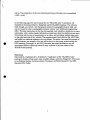
ABSTRACT
The Skagerrak International Experiment (SKAGEX) was carried out in the SkagerrakKattegat in the period of 1990-1991. It involved four field surveys with up to 17 vessels
perfonning simultaneous oceanographic measurements at sea. The resulting data set
covers a wide range of environmental parameters from hydrography to marine chemistry
and biology. It comprises results from more than 2000 oceanographic stations with
sampies being taken at multiple depth levels. In order to make this huge dataset easy
accessible to all scientists participating in the experiment a software package has been
written that integrates functionality of a database with the presentation methods typical for
oceanographic applications, such as XY charts, sections, time plots and horizontal
distributions (maps).
Thls presentation, based on the user's manual ofthe "SKAGEX Atlas" demonstrates its
basic features and gives examples ofits use in studies on synoptic scale variability in
Skagerrak and Kattegat. It indicates also in what ways the use of this software may be
extended to other oceanographic datasets.
Introduction
The international marine experiment in Skagerrak (SKAGEX) was conducted in aseries
of field surveys between May 1990 and May 1991. During each survey scientist from
nine nations, from boards of the research vessels, were conducting an extensive "
programme of the in situ sampling that included hydrophysical, chemical as weIl as
biological parameters. One ofthe main aims of SKAGEX was the recognition of the
time variations of the Skagerrak-Kattegat watl~r masses in the short, synoptic scales. In
accord with that, a regular sampling programme covering carefully selected net cf stations
was being carried out once in every three days. There was eight main sections spanning
the Danish, Swedish and Norwegian coaSts, beginning from the whereabouts ofthe Laso
Island in the East towards the western-most section extending into the North Sea domain.
On all sections the vessels operated simultaneously with spacing between the stations in
the range of 5 nautical miles. In addition to that, in particular during the SKAGEX I
(May-June 1990), other ships not involved, directly with samplirig on the sections, were
collecting sampies at additionallocations , bringing the total number of ships at sea during
the most sampling-intensive days to the 17. The observations were also made in the days
between the obligatory sections. The was no detalled scheme of investigation dtirlng these
times~ each scientific crew carried out the progiäm according to their national agenda,
still the data than collected were made available to all participating piuties.
Evaluation of sampIes and primary processing of on-board data were worked up by the
participating groups. Tbe CTD casts reduced to one metre bins and the water bohle level
data for chemistry and biology were submitted to the leES data management group where
they underwerit the final quality check and were put together to form a coherent database
to be released to the all member institutions. This scheme worked weil and timely, so that
by November 1991, only after four months after the last field survey, the diskettes
containing full SKAGEX dataset with hydrographie and chemical data plus chlorophyll,
with all surveys ineluded, had been supplied to prinCipal scientist from the member
institutions.
Having the database compiled the objectives were set for scientific evaluation ofthe data.
Whilst the most evaluation work
to be carried by separate scientific groups in their
base laboratories, in severaI topics a elose cooperation .at intemationallevel coritinued.
Artlong such topics were the studies on överall circuhition pattern iind hydrographie events
taking place during SKAGEX. To a support this work the author proposed the üse of an
already existing custom software package, developed at 10 PAS, specially designed to
automate the process of the oceanographic cruise results reporting The proposition was
accepted by the study group during the group meeting in November 1991. In April 1992,
the first version of the package containing the SKAGEX dataset plus presentatio~
software was ready for distribution. It was soon followed by a draft copy of an atlas
showing the daily variations cifthe major parameter fields during SKAGEX I. It contained
over 1000 maps with the horizontal distributions oftemperature, salinity, densitY, nitrate,
nitrite, silicate and phosphate at several depth levels ranging from the surface doWn to 200
was
2
•
'.
'-i-,
•
) I
•
metres. The preparation ofthis atlas incIud~ng printing and binding was accomplished
within a week.
.
In the following pages the userls manual for the "SKAGEX atlas" is presented. All
examples in the manual relate to Skagerrak and the SKAGEX database. The software
itself, though, was written with the general model of oceanographic data in mind, and
may be reused for other oceanographic datasets without much additional programming
eifort. The basic requirement is that the data supplied must resemble a simple one-to-many
relationship, with astation header infonnation containing at least the platfonn/event name,
the location and the time of measurement as an index, and pertaining multiple data cycles
on the right hand side of the relation. The program imports such data for flat ASCn files
and builds in a relational database in its own format. The author has tested this system on
several datasets; one example of its use will be shown on the poster session during the
lCES meeting. [Ostrowski a1. all 1993]. However, the import facilities are not yet
documented neither sufficiently tested for their inclusion in the next release of the
SKAGEX atlas package.
References
Ostrowski M., Danielssen D.S., Svendsen E. "Application ofthe "SKAGEX Atlas"
package in studies oflong water mass variability along a section in Skagerrak", The poster
to be displayed during the theme session "Computers in Fishery Researc.h", the ICES
Meeting 1993, Dublin
3
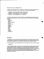
About this version of Skagex Atlas
Version 3 ofthe "SKAGEX ATI..AS" is based on the results from the experiment downloaded from
ICES database in January 1993. The data are subdhided ioto the four following categories:
•
•
•
•
SKAGEX I
SKAGEX TI
SKAGEX III
SKAGEX IV
ith 1586 stations from 18 May to 25 June 1990
ith 127 stations from 10 to 17 September 1990
with 98 stations from 12 to 20 January 1991
....ith 299 stations from 17 to 20 May 1991
In contrast to previous versions. liere is no separation into chemica1 and physica1 datasets; all data
relevant to a selected station are accessible in the same database. The field stnleture ror each database is
given below:
Depth
Temperature
Salinity
Potential temperature
Density
Potential density
Oxygen
Phosphate
Phosphorus
Silicate
Nitrate
Nitrite
Amrnonia
Nitrogen
Chlorophyll A
Installation
The package runs on PC machines with processors 80286 or higher. All programs and data take about
12 MB memory on your hard disk. The package can be executed even on small notebooks provided that
there is enough conventional memory (more than 560 KB) and a numeric processor is installed.
To instaH the package, insen the disk labelIed #3 (not #1) into floppy drive, log onto that drive and type:
UNPACKX:
where X: stands for the letter ofyour hard drive. The decompressing utility (UNZIP.EXE) will ask you
to change installation diskettes three times more. The atlas creates a path SKX on the root directory of
your hard drive. To nm it one should change to this path and type the command: SKX . Always nm
SKX program from this directory. The atlas program uses a large portion of conventional memory during
execution, and its is not safe to run it from within the memory resident utility such as Norton
Commander or XTPRO. The package behaves correctly under Microsoft Windows 3.1, only when is
executed in fuH screen mode.
4
•
The new version ofthe Atlas similarly to older ones requires the SURFER package (Golden Software
ver. 4.0,1989). lfthis product is not present or not registered. the program issues the follo\\ing wamirig:
Error during initialisation, invalid item: PRN
To register SURFER" go to [OPTIONS I DIRECTORlESJ and type in its proper path.
Basic operations and screen layout
The main screen ofthe atlas consists ofthe top menu bar from where commands are selCCted, and the
status line at the bottom showingnames ofseveral kcys used for accessing some ofthecommands
immediately. In the centre of the screen a \\indow is displayed \\ith information on hydrographie
st:itions during SKAGEX. Vou can zoom that window by pressing F5, drag it around the screen. shrink
or e.'q)3Jld. and close (remove from the screen). The WINDOWS menu on the top bar does operations on
\\indows, but most ofthese functions can be accesSed faster by tising so-callCd "hot keys". Names ofhot
keyS are listCd to the fight ofthe appropriate coinmand from the menu bar. For exarnple to dose a \\indow
yoti should press Alt-F3. To access the main menu press F1 0 ~ or hold Alt key while pressing the focUsed
letter of an item you arC going to select. To quit the program press Alt-X or go to the SYSTEM, EXIT
menu command on the top menu bar. TIlis version ofthe progiam is provided \\ith the context
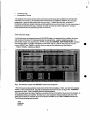
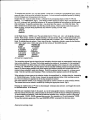
senSitive help SyStem which can be invokC:d by pressing F1. Fig. 1 shows the main progiain screen of
the
atlas \\ith the WINDOWS menus popped
•
Fig.l Tbe main screen of .Skagex atlas package showing
information window in the background
•
Work with the atlas is subdivided inta the threC distinet stages:
data selection stage
5
•
•
processing stage
presentation of results
,
Tbe databases ofthe atlas contain almost all physical and chemical data available from the SKAGEX
experiment Tbe access to the required portion of this dataset is Possible by definition of a time span.
geographical range and ship name (data selection stage). Selected data are then processed as
horizontal distributions (maps), tninsects and time-depth plots (processing stage). In most cases resu1ts of
processing are stored to files and to examine the result one needs to ca11 the appropriate ';e....ing or
printing function after the processing (resu/t presentation).
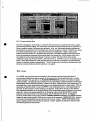
Data se/ection stage
As the first step in an attempt to access the SKAGEX datasel one must select the variables, time span
and location for the data. For making selections the atlas provides a special . selection windeiw. To
activate this v.indow, you need to press Alt-F9 or select the QUERlESt NEW INVENTORY command
from the main menu. A ....indow will appear on the screen. (fig.2). It has its own menu bar ....ith t\\"o
menus: SELECT and FILES, a list box where )'OU can see your selections and four buttons:
Insert, Modify, Oelete and Open.
•
•
Fig.2 Tbc selection window with SELECT menus in thc foreground.
Makc:
Tbe tirst step in the data selection is thc choicc of thc relevant database.
your choicc by pressing
Alt-Fa or AIt-e followcd by D and pick the appropriatc item from thc list: in (tig.3) Tbe VARIABLE
command will show a list ofVarlables from the selected dat.abase.
Tbere are cases when the ordcr of stations on invcntory Ust has to be different from th3t of the databasC. In
the databases all data are sortcd by thc ship namc, than subsequent stations increasc with
This
order may bc altercd, by selection of one ofthe options availablc on the SORT ORDER selection list.
Tbe following orderings are providcd:
time.
time
longitude
latitude
6
latitude than longitude
longitlide than latitude
longitude than time
latitude than time
longitude then latitude than time
latitude then longitude than time
•
Fig 3. Selection of database from the seleCtion window
•
Fig.4 A dialog for seieCtion of ship, time spaii and geographie3I range
7
To complete the seiection. one must also specify a time span. a rectangle in geographical Space. and the
narnes of ships, which are to be included in the search. You can construct compound queries by chaining
several rectangles and time periods to the one list.
Suppose that one wants to select the data coUected by all participating ships on May 27 1990. By
pressing I or Insert button. (fig.2), a new dialog window appears on screen (figA) The asterisk '*' in
the min (minimal) field S)mbolises selection of all stations regardless ofheir position in the time-spaceship coordinates. To specify a particular date one should alter the value in the Date min field • The
date is entered in the inverse order: year first than month and day. There must be exaetly three pairs of
digits per entry, each pair being separated by any character S)mbollou "ish. Thus:
900527
900527
90/05/27
are all legal whereas 90052 is not. The same holds true for Time and Lan, Lat (lon~ttide, latitude)
entries. There always must be six digits denotirig in the case of time: hours. minutes and secclnds and in
the case of geographica1 position: degrees, minutes and tenS of aminute. The ... max fields may stay
blank. By setting them one selects, a date, time ofthe day , longitude or latitude ranges for the selection,
rather than single values. Valid ship names for this version of SKAGEX atlas are:
ARGOS
HUMBOLDT
ATAIR
HYDROMET
TISELIUS
J.HJORT
A.VEIMAR
LTITOV
DANNEVIG
OCEANIA
G.O.SARS
SIEDLECKI
THORSON
SVANIC
BRAARUD
MOSBY
All must be in capitalletters.
•
Twa rernaining objects from the input form are included to limit the search to oceanographic stations truit
meet certain conditions. The item: Query type specifies the relation of the selection to the variableS Ir
all recs condition is in effect a.ll data sets \\i11 be included regardless of the values set in the v:mahle box
( Fa key). On seleded vars, only the stationS with the checked variables present are included during the
search. On Non-missing condition only those stationS and selected variables arC included that have no
missing values embedded inside their dataSets. Records condition liniits the search to chosen record
range from the currently activc database. When it is blank all the database content will be Searched.
a
When selection is done retum to the selection window is accomplished by clicking either the Ascending
or Descending button. The first forces. folward. the second backw3.rd order of the resulting inventory
list. The new selection is appended to the list that occupies the cential
pan·ofthe selection window. A bar running across this!ist shows in inverse an item currently selected.
Tbe selected item can be deleted or modified by clicking the appropriate button. (fig.3)
Pressing the Open button or 'P' letter on the ke}'board terminates wlta selection and triggers the search
for selected stations in the database.
Tbc first and immediate result of this search is a list of oceanographic stations matc:hing ihe selection.
Only the stations from this list. called hereafter the iß\'Cntory provide the data for subsequent processing.
Ta avoid repetition of selection , each time the ci3ia aie requested they should be savCd to ä file before
the data seareh. FILES t SAVE command lets you sa\'e the selection as a file With extension *.MQR.
To load that selection again press F9 or use QUERIES,OPEN command from the ßiain menu.
Data processing stage
8
•
7
,
The stations conforming to the selection condition are returned in the inventory window which
occupies the same position on the Screen as the former selection \\'indow from where the search was
called. Tbe window displays a list of selected oceanographic stations. Tbe horizontal bar pointS to a
record currently selected (fig.5).
Fig 5. Invemtory window with station selection for datall3Se: SKAGEX I, vessel Oceania.
date 27 05 1990. ",'ith SHIP TRACK menus in thi: foreground.
•
All data processing operations are relevant to the displayed selCction of Stations. The folloWing
operations are available:
.
• Viewing the map ofPositions ofall the Stations incbidCd in the selection. (SHIP TRACK menus)
•
Viewing the station 's data as numbers on the screen, (RECORDS menUs)
• Plotting twO selecied variables simultaneously,(RECOROS menUs).
• Storing station data to a file,(RECORDS menus)
.
• Making a verticiU section ofa variable along the j)ath a10ng all Siätions from the inventory !ist
,(SECTIONS menus)
• Creatlng a map at chosen depths for a seiCeted variable, MAP menus)
•
Storing current settings ofim-entory whidow (variable selection, plot ws choice etc.) to *.MQR
-file.
SHIP TRACK menus
This menü displays
on the map the positions of ships included in the inventory list. The pictUre
can be stored to a file in the SURFER compatible format and used aS hard cOpy (STORE command)
9
----~----
'{
R-e:
.88~/.875.
90-05-27
08:00:0 /
90-05-27
22:00:0
Fig.6. Ship's track ofOceania on 27.05.1990. The result of SHIP TRACK, VIEW conunaßd.
RECORDS menu
The record menus provides operations on a single oceanographic station seleetion. The stauon is
seleeted by moving a selection bar up and down the inventory !ist. Ta view data in the numeric form press
the VIEW DATA command. The STORE DATA command allows you to store the data from a seleeted
station in a text file. The comrnand OPTIONS, MISCELLANEOUS from the main menu 3.f:reets the
output by forcing an appropriate separator between the nurnbers and symbol replacing missing data
values. Ta obtain the file in *.CSV format, comPatible with popular spreadsheet packageS one should
select a comma as delimiter. The VARIABLES command selects variables for output, those unseleeted
wiU not appear on the output
,
PLOT comrnand displays a pieture containing two X-Y plots for any eombination ofvariables accessible
in the database. Selection of these variables is made through the SELECT AXES eommand. SETUP
CHART sets options for axis orientation. line style ete. The plot can be stored in SURFER compatible
format (STORE PLOT).
•
a
SECTIONS menu
This menu provides methods for the ereation ofvertical section or time plot along the route or \\ithin the
time span from the inventory Iist. The order of stations to be plotted will be the same as that of the
inventory, and should be designed during the data selection stage. There is no limitation to (me-shipsections only. Time-depth diagrams are also possible. ifthe selection is confined to one station at different
dates. Selection ofthe variable for transect and interpolation method is made through the SECTIONS
menu Vertical axis is always set to depth; the horizontal axis can be either time or distance. Interpolation
is done by the SURFER package and the result is written to a file. In the case of sections of the best
results seem to be obtained when using the minimum curvature interpolation method. Berore ~ triggering
interpolation (MAKE comrnand) one should select variable to display (SELECT VARIABLE
eommand) and set appropriate ranges. Figure 7 shows the layout of the selection form whieh appears in
response to the RANGES command:
a
10
•
·.
'.
":Fig 7. Transect selection·form.
The fonn is ärnuigCd in three columns : the first for the horizontal axis, second for the vertical and the
third showing selected variables. The item scale .selects the size of the transect pietUre in centimetres or
forces a constant number ofkilometres per centimetre. step setS the distance between neighboUrlng
descriptions in the selected units. On the depth axis, the unitS ärealways in meterS. The grid item selects
the number of grid points along the horizontal and depth axis resPeetlve1y . Higher values usu3..Ily
produce more exaet rCsuIts, but calCuIation takes more time. The Depth column has also min and max
entries for selectiog the minimum and maximum depth of a transect and a break option which teIls at
what depth the vertici.l scale should chaiige.
obtain the upper 100 meters ofthe water column
enlarged five times, one should set break to 100 arid rate to 0.2. If break is set to 0, no chaßge iri scale
ocetirs . In the third column min, max and step items set a minimwri, a maXimum and a step bCtl\'een
isolines of a selected variable correspondingJy. The err (relative error) iteni h3S the meaning only when
minimum Curvature method is selected, otherwiSe it is ignored
Ta
,./
MAP menus
•
The MAP S menu provides tools and methods for the coriStruction of horizontal distributions of
enVironmentalvariableS from stations present in the im'cntory list. The process begins With
"slicing" operation..The user selectS via RANGES\REFERENCES command the reference vmable.
usually the deptb. Tbe databasC engine program from the atlas pack3ge fulfils the requeSt by browsing all
oceanographic stations inside the inventory Window at the 8iven reference level. If the requcSttd level is
not present thari a value interpolated linearly from the two neighbouring layers istaken instead • When all
<1313 points are fowid thei-esult is sent to SURFER to be interpolated onto an evenly sPacec1 grid and
the.result. of that is plotted in tenns of isolines. The position of the grid on the map, its size and few
other par3meters necessary for the proper definition of the interpolation process are storCd in the SCKalled
region file. The file with settings adjusted for the Skagerralc region, named SKAG.REG is already
Prepared on the horne directory ofthe atlas package. (Fig. 8) This file must always be assigned to
inventory window before a map can be produced. (ASSIGN REGION command).The .MAKE command
triggers the map creation proeess. There are two variants of this command. MAKE FOR ALL produces
ooe map for an oceanographic stations sele(:ted to the inventory window. MAKE FOR EACH instead
makes a separate map for each line ftom the selCction \\lndow. Suppose that dUring the selCctlon Stage
the following lines have been enterl:d:
sa-called
11
.,
Rec:
.298/.t33~:.
90-05-26
58·00~~:tOO:":':=E~--0-8-*""OOL.'E
Ot:OO:O /
90-05-28
20:00:0
·OO'H
tO*OO'E
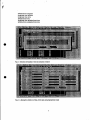
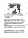
Fig.8. Ship positions of all the stations occupied in Skagerrak between 26 and 28 May 1990. The
rectangJe surrounding the selection limits the region in which rnaps \\ill be plotted. The region shown
here has been defined in the file SKAG.REG and displayed on screen using VIEW ASSIGNED
REGION option from the MAPS menus.
•
{*;*;*;900604:900S06}
{*;*;*;900607:900609}
The first line stands for selection of all vessels in the database between 4th to 6th June 1990, whereas the
second between 7th and 9 June. When this query is sent to the MAKE FOR ALL command than only
one rnap with averaged resulls from all casts from 4th to 9th June \\ill be made. The MAKE FOR EACH
command \\ill create the two separate synoptic rnaps ofboth periods respectively. This comrnand is very
convenient when large number of rnaps to show synoptic variability is required. The query file
LEGS.MOR provides the selection of stations allowing for creation of the rnaps covering all SKAGEX 1.
Thc rnaps are made in two forms: as isoline plots and colour raster rnaps displayable on the computers
screen. None ofthese are shown after the interpolation. One must use one ofthe commands from the
CHARTS menus on the rnain menu bar to display the results on the screen or plotting device.
FILE
menus
SAVE and SAVE TO comrnands allow to store the euerent state of an inventory window into a selection
file (*.MOR). Next time such a file is loaded all the assignments and setting applied to this \\indow so far
will be restored. The GET #REC command copies parameters of the oceanographic station pointed by
the selection bar to the program clipboard from where they can be retrieved into another selection window
on the screen.
Presentation ofresults
The results of transects and rnaps are stored in files under names given by the user. The group of rnaps
created \ia MAPS, MAKE FOR EACH cornmaßds are accessible through a special driver file \\ith
extension (*.LOG) . To display 00 the screeo or to plot a single map or transeet use the comrnands from
CHARTS menus on the rnain menu bar. Each ofthe commands from this menu asks for the file name of
an item produced during the data processing stage and starts appropriate plotting routine.
help
The
12
•
·.......
'{
Syste~ invoked by pressing F1 when CHARTS menus has been selected gives detailed instruction on
how to use these commands.(Fig.9).
Ir. the ship track from fig.6 waS used to create avertical section of nitrates aiong "Oceania" route from
27.05.1990 and the result is stored under the name OCN03275.PLS then ha"e this resUlt displayed
on the Screen select VIEW SECTION comma.nd arid pick this näIDe from all files \\ith the
extension *.PLS (Fig.l0). Fig. 11 shows the resuIting plot
to
•
Fig. 10. Selection ofthe file OCN03275.PLS
route on 27.05.1990.
13
c
"
... ....
....
•.•
....
I ....
.
I.
, \",.1 .-,
.~
•
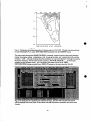
Fig. 11. Distribution of nut:icnls along the r/v Oceania route on 27.05.1993. Tbe plot was retrieved from
the file OCN03275.PLS using VIEW SECTIONS command from the CHARTS menUS
Tbe maps created through the MAKE FOR EACH command cannot be found on the current directory.
Instead the program creates a subdirectory \'11th the user given name and a special driver file \'11th the
extension *.LGT. All maps resulting from this comrnand are put to that directory being ~ven numeral
file names increasing \\ith the order of their creation i.e. 001.PLM, 002.PLM, ••. . To view such a
collection on the computer screen. give the name of the proper driver file in VIEW
DISTRIBUTIONS dialog accessible from RESULTS menus on the main menu bar. (Fig.12).
14
•
900528: 900528 000001: 235858
•
S6.0~~:!OO:::-:'::E:----08-.-00,.1..:'E
10·00·E
Fig. 13. Distribution ofnitratesinterpolated from alt datasets available between 26 and 28.05.1990
R_ _ :
8OO810:S00812 DDDODl:235BSS
Fig. 14. Distribution of nitrate~.interpoiated from all dataSets availabte bet\·.een 10 and 12.06.1990
15
'{
Tbe prograrn ",iU t.han show in colours the horizontal distribution ofinterpolated parameter on top ofthe
contour rnap of Skagerrak.
Pressing the space bar moves to a new distribution. Fig. 13 and I ~ show a sampie distributions of nitrates
at the depth of 30 meters obtained when a driver file N03-30.LGT is used in the dialog bOx from fig.
14.
'Vindows management
~Vjndows
Most ofwhat )'ou see and do in the prograrn manager happens in a "indow. A window is a Sereen area
that )'ou can open. elose, move, resize, and overlap. You can have up to nine \\indows open in the
prograrn manager, but only one \\indow can be active 3t any time. Tbe active ",indow is the one that
you're currently working in. Any comrnand from the loCal menu bar you choose or text you type generally
applies only to the active window.(Ifyou have the same queI}' open in several ",indows, the action ",iU
apply to the file cverywhere that it's open.)
You can spot the active window easily: H'S the one \\ith the double-lined border around it. Tbe active
",indow always has a elose box in the upper corner. IfyoUr ",indows are overlapping, the active "'iodow is
always the one on "top" ofall the others (the front most one).Tbere are several t)-pe8 of",indows, but most
of them have these things in common:
•
•
•
•
a title bar
a elose box
a window number (I to 9)
Tbe dose bor of a ",indow is the box in the upper left corner. Click tbis box to quickly elose the
window. (Or ehoose W1NDOW , CLOSE or press Alt-F3.) Tbe lilie bar, the topmost horizontal bar of a
window, contains the namc ofthe window and the \\iodow number. You can drag the title bar to move
the windowaround. Tbe zoom bor ofa window appears in the uPPer right corner of a data "'indow. Ir
the icon in that corner is an up armw, you can elick the armw to enlarge the window to the largest size
possible. Ir the icon is a doubleheaded armw, the ",indow is alreadY 3t its maximum size. In that case,
clieking it returns the window to its previous size. To zoom a daci window from the kC)'board. choose
W1NDOW , ZOOM, or press F5. Datl windoM also riiturii to the ußzoomecl state following eaeh call to
the database engine, or graphie routines. A window number is displayedß the upper right border. You
can make a windowaCtivc (and thereby bring it to the top ofthe heap) by pressing Alt in eombination v.ith
the mndow number. For example, if selection mndow LEGS.MQR Window is #S but has got buried
horizontal or vertical bars that are
under the other mndoM, AIt·5 brings it to the front. Serail bars
visible on the battom and right sides ofan aciive data mndow. YOll use these bars ",ith a moUse to seroll
the cöntents ofthe window. Cliek the arTeW at either end to seroll one line at a time. (Keep the mouse
button pressed to scroll continuously.) YOll can eliek the shaded area to either side ofthe seroU box to
scroll a page at a time. Finally, you can drag the seroll box to any spot on the bar to quiekly move to a spot
in the mndow relative to the position of the seroll box.
You can drag any corner to malee a window larger or srnaller. To resize using the kC)'board. choose
SlZE,MOVE from the WlNDOW Ctr1·F5.
arc
16
•
"