Download Basic global prediction tool and user manual

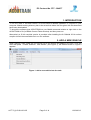
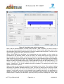
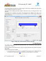
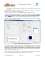
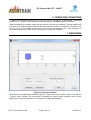
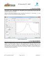
EC Contract No. FP7 - 284877
Virtual certification of acoustic performance for freight
and passenger trains
D 4.2 – Basic global prediction tool and user manual (interim)
Due date of deliverable: 30/09/2012
Actual submission date: 12/03/2013
Leader of this Deliverable: David Thompson ISVR
Reviewed: Y
Document status
Revision
Date
Description
1
26/02/2013
First issue – failure to upload in the repository
2
26/02/2013
First issue – failure to upload in the repository
3
26/02/2013
First issue
4
12/03/2013
Revision including comments from quality review
5
12/03/2013
Final version after TMT approval
Project co-funded by the European Commission within the Seven Framework Programme
(2007-2013)
Dissemination Level
X
PU
Public
PP
Restricted to other programme participants (including the Commission Services)
Restricted to a group specified by the consortium (including the Commission
Services)
Confidential, only for members of the consortium (including the Commission
Services)
RE
CO
Start date of project: 01/10/2011
Collaborative project
Duration: 36 months
EC Contract No. FP7 - 284877
EXECUTIVE SUMMARY
The objective of this task is to implement a framework for a simple global simulation model based
on the minimum requirements and input/output data defined in Task 4.1. As input this global
simulation tool takes data describing the various sources on a train (sound powers, possibly
directivities) along with geometrical data about the sources, the receiver and the ground
properties. From these input data predicts the evolution of the pass-by sound level (overall and in
one-third octave bands). The development of this simulation tool is based on the required
input/output defined in task 4.1
The purpose of this simulation tool is to demonstrate the method of prediction required as part of
the virtual certification process so that third parties can use it.
ACT-T4_2-D-ISV-001-05
Page 2 of 14
12/03/2013
EC Contract No. FP7 - 284877
TABLE OF CONTENTS
Executive Summary ...................................................................................................................... 2
List of Figures ............................................................................................................................... 4
1. Introduction ............................................................................................................................... 5
2. Add a new vehicle ..................................................................................................................... 5
2.1 Add Sources ....................................................................................................................... 7
3. Manage the train ....................................................................................................................... 9
4. Add rolling noise ..................................................................................................................... 10
5. Test site definition ................................................................................................................... 11
6. Operating conditions ............................................................................................................... 12
7. Receivers ................................................................................................................................ 12
8. Calculations ............................................................................................................................ 13
9. File management .................................................................................................................... 13
10. File format for uploading ....................................................................................................... 14
10.1 Sound powers ................................................................................................................. 14
10.2 Roughness ...................................................................................................................... 14
10.3 Monopole to dipole ratio .................................................................................................. 14
ACT-T4_2-D-ISV-001-05
Page 3 of 14
12/03/2013
EC Contract No. FP7 - 284877
LIST OF FIGURES
Figure 1: Add a new vehicle into the train. .................................................................................... 5
Figure 2: Describing new vehicle parameters................................................................................ 6
Figure 3: Right click on the wheelset to edit its properties. ............................................................ 7
Figure 4: Defining new source parameters. ................................................................................... 8
Figure 5: Right click on the vehicle body to edit all vehicle properties, including sources related to
the vehicle. ............................................................................................................................ 9
Figure 6: Defining a rolling noise input for a specific wheelset type. ............................................ 10
Figure 7: Test site geometry and ground impedance properties. ................................................. 11
Figure 8: Receivers position. ....................................................................................................... 12
Figure 9: Results view. ................................................................................................................ 13
ACT-T4_2-D-ISV-001-05
Page 4 of 14
12/03/2013
EC Contract No. FP7 - 284877
1. INTRODUCTION
To run the code of this beta version of ACOUTRAIN a Matlab installation is required in your
computer. Matlab working directory has to be set as that where the files given with this document
have been downloaded.
To launch the software type ACOUTRAIN on your Matlab command window or right click on the
ACOUTRAIN.m file (in Matlab Current Folder window) and then press run.
Alternatively a 32 bit compiled version is provided: after installing the 8.0 Matlab 32 bit runtime
compiler launch the executable file to run the software.
2. ADD A NEW VEHICLE
When starting a new model the first vehicle has to be defined and added to the train. From the
menu bar press ``Create'' and then ``add Vehicle'' (see Figure 1), the window shown in Figure 2
appears.
Figure 1: Add a new vehicle into the train.
ACT-T4_2-D-ISV-001-05
Page 5 of 14
12/03/2013
EC Contract No. FP7 - 284877
Figure 2: Describing new vehicle parameters.
Here it can be decided whether to create a new vehicle or load an existing. In order to create a
new one the main parameters has to be inserted in the ``Define vehicle geometry'' panel. Once
the parameters have been inserted press the ok button located inside this panel. The axes on the
right are then updated and other panels are activated.
Within ACOUTRAIN the wheelsets are characterized by their position on the vehicle (x
coordinates of the wheelset relative to the first end of the vehicle) and by their type (or the set
they belong to). Before adding a wheelset it's therefore necessary to create a wheelset type.
When starting a new model no types are available, they can be created through the functionalities
given in the ``wheelsets type'' panel. The wheelset type contains the information about the wheel
radius and about the results coming from TWINS calculation (these will be loaded later on). To
create a new type enter the wheel radius associated and the name of the set, then press the
button ``Create new''. The list of available sets will be updated. The existing sets can be then
edited or deleted as required.
When at least one set exists the wheelsets can be added to the vehicle. Two modes of adding
wheelsets are available: standard and one by one. The first one allows one to enter the number
of wheelsets existing on the vehicle and defining then the boogie wheelbase and boogie centre
distance. In this mode only two or four wheelsets can be added. Note that if two wheelsets are
added the software will ignore the datum boogie wheelbase. When pressing the button ok the
software asks for entering the wheelset's type they belong to before updating the vehicle. Both
ACT-T4_2-D-ISV-001-05
Page 6 of 14
12/03/2013
EC Contract No. FP7 - 284877
the wheelset position and type can be edited using the context-menu available when right clicking
on each wheelset in the axes (see Figure 3).
The second mode of adding wheelsets consists in adding them one by one using the button ``Add
wheelset''.
Pantographs can be added to the vehicle. The pantograph to be added at this stage is not
representative for its acoustic properties but its visualization on the vehicle image can help the
sources positioning.
Figure 3: Right click on the wheelset to edit its properties.
2.1 ADD SOURCES
The software allows now to add some general sources. The ``add sources'' button opens the
window shown in Figure 4.
At first the frequency range has to be set, all the files to be loaded within this window must match
these range.
Different source types are available:
•
As a default setting a Point Source is proposed. Sound power can be loaded from a file
according to the format shown here; by default a unit power spectrum is proposed.
ACT-T4_2-D-ISV-001-05
Page 7 of 14
12/03/2013
EC Contract No. FP7 - 284877
•
Alternatively the Area Source will distribute points on a given surface on the receiver side
of the train.
For both these sources the ``aerodynamic source'' option can be chosen, in this case a
dependence of noise with speed has to be defined.
The source directivity is defined as a ratio between monopole and dipole behaviour.
Monopole to dipole ratio can be modified by the ``Reset all'' button in the Standard directivity
panel otherwise a different ratio value can be set per each frequency by loading an appropriate
.to file (click here to open an example and see section 10). Dipole axis can be modified by
rotating it around the x axis and then around z axis from its original position (parallel to z axis).
Directivity can also be described by the user in a text file in terms of noise levels at certain angles
and radii in spherical coordinates system.
Figure 4: Defining new source parameters.
By pressing ok (bottom right) the current window is closed and the previous one is restored. The
created sources can be positioned on the vehicle by left clicking on the vehicle axes. Once the
sources have been positioned a context-menu allows their position to be modified, they can be
switched off/on, deleted or edited as necessary. To help the right clicking on the source the
vehicle body can be temporarily made invisible. All the sources and wheelset's type can be listed
with the ``Source list'' button (top right).
The procedure of adding sources on a vehicle can be repeated as many times as it is necessary.
The vehicle can be saved as a Matlab file and loaded again for other models.
ACT-T4_2-D-ISV-001-05
Page 8 of 14
12/03/2013
EC Contract No. FP7 - 284877
3. MANAGE THE TRAIN
When all the required wheelsets and sources have been added the vehicle is ready to be placed
in the train. After entering the vehicle position press the button ok (right bottom), the current
window is closed and the main one restored with the new vehicle available. By right clicking on
this one several functionalities are displayed, the vehicle can be copied, edited, moved or deleted
(Figure 5).
Figure 5: Right click on the vehicle body to edit all vehicle properties, including sources
related to the vehicle.
The copy option will copy the vehicle and position it at the right of the existing one.
To move a vehicle from its position on a train to another one choose the move option from the
menu and then left click on the gap between two other vehicles where the selected vehicle has to
be moved.
By choosing the editing option the window used to create the vehicle is reopened and all the
described functionalities are again available.
The ``List source`` will again display all the sources and wheelsets of the vehicle.
ACT-T4_2-D-ISV-001-05
Page 9 of 14
12/03/2013
EC Contract No. FP7 - 284877
4. ADD ROLLING NOISE
Figure 6: Defining a rolling noise input for a specific wheelset type.
The ``add rolling noise'' item in the ``create'' menu allows to attach to the existent wheelset types
the rolling noise power components (Figure 6).
Within this GUI the sound power levels can be visualised in terms of acoustic power. If necessary
they can be removed from the model.
There are two different ways to load sound power into the software, in both the cases the sound
powers are meant to be calculated with a unit (1 m) roughness input.
•
•
Loading single files powers. Wheel power, rail power and sleeper power .txt files can be
selected after clicking the button ``load text files''. File format is similar to the point
sources, with the peculiarity that the first string in the file must be ``wheel'', ``rail'' or
``sleep'' according to the power component the file refers to. It is not necessary to specify
the correct speed since roughness and contact filter will be defined in the tool according to
the speed specified in the window ``Operating conditions''. However in the position where
the speed is normally defined inside the .txt file a number is required, but it won't be read
by the tool. Writing for example ``0'' is an allowed option. See section 10 for further details.
In the wheel power file the first line after the frequency vector must be the contribution of
the axial motion while the second line of radial. An example is available herein the rail
power file the vertical power component comes first one and the lateral afterwards, note
that if the rail power have been calculated per wave component then both the propagating
and decaying waves should be accounted by adding them. Example available here.
There must be only one power component in the sleeper power file. Example available
here.
Selecting a TWINS folder. If the outputs of the software TWINS are available, then the
``Select TWINS dir'' button allows browsing to select a TWINS model folder (outputs from
ACT-T4_2-D-ISV-001-05
Page 10 of 14
12/03/2013
EC Contract No. FP7 - 284877
TWINS 2.4 have been tested so far). Sound powers will be detected inside the folder and
loaded along with the Track Decay Rates.
Contact filter is always accounted adopting the train speed set in the ``Operating Conditions''
window, while roughness can be set via the radio buttons:
•
•
•
•
unit: 1 µm roughness per each wavelength;
TSI: the limit curve defined in TSI is adopted;
Load one file: the combined (wheel and rail) roughness is contained in one single file
(extension .to). See section 10 for format explanation
Load two files: wheel roughness and rail roughness are loaded separately; the software
will add them up. Same .to format file is to be used.
Note that the sound power levels won't be uploaded until the ``Attach acoustic power'' button is
pressed.
5. TEST SITE DEFINITION
Figure 7: Test site geometry and ground impedance properties.
To define the test site the ``Test Site Definition'' item in the ``Create'' menu gives access to the
GUI showed in Figure 7.
The geometry can now be set only in terms of distance between the main reflecting ground and
the top of the rail (i.e. the vertical origin of the reference system).
The ground can furthermore be defined as rigid or reflecting (Delany Bazley, Miki and HametBerangier models are implemented in the code). Calculations without ground can also be
performed.
ACT-T4_2-D-ISV-001-05
Page 11 of 14
12/03/2013
EC Contract No. FP7 - 284877
6. OPERATING CONDITIONS
To define the operating conditions of the train the type of the test has to be defined (``Operating
conditions'' in ``create'' menu). Passby at constant speed or standstill mode are allowed.
When considering the passby mode the test duration can be here modified. The test duration will
also define the relative position between the train and the receivers x coordinate. This latter is set
to be in front of the middle of the train at half of the test duration time. This parameter is
somewhere displayed in the software windows but it cannot be modified.
7. RECEIVERS
Figure 8: Receivers position.
Receivers can be added and edited through the ``Define receivers'' function (Figure 8) inside the
``Create'' menu. Default TSI positioning is available but further single receivers can be input.
Right click on the receivers shown in the figure for editing and deleting.
ACT-T4_2-D-ISV-001-05
Page 12 of 14
12/03/2013
EC Contract No. FP7 - 284877
8. CALCULATIONS
Once all the previous parameters have been suitably set, the software is ready to perform the
calculations. Go to ``Calculations'' ``Calculate'' to launch them. Before running, the time
increment can be here modified.
When the waiting figure disappears press ``exit button'' and then go to ``Calculations'' ``View
Results'' to plot the sound pressure quantities (Figure 9).
Figure 9: Results view.
9. FILE MANAGEMENT
When the software saves the model both the geometrical/physical and numerical results are
stored in the indicated folder. When the model is loaded if valid results are found the user is
asked to open the model in editing or non-editing mode. In non-editing mode only few
functionalities are available preventing thus undesirable modifications, while anything can be
done when edit mode is activated. Note that the results will be modified only after the RUN button
is pressed inside the calculate GUI.
ACT-T4_2-D-ISV-001-05
Page 13 of 14
12/03/2013
EC Contract No. FP7 - 284877
10. FILE FORMAT FOR UPLOADING
10.1 SOUND POWERS
It's a .txt containing a matrix of strings and numbers. The elements of the matrix should be
separated by the character ``Tab''. When the power file does not describe power due to rolling
noise, then the first column specifies the sound power speed dependence: the first element
should be the string ``speed'' then all the speeds values. In the first row, starting from the second
element, the third octave centre frequency value should be reported. All the other rows describe
the sound power levels in third octave band for each speed defined in the first column. An
example is available here.
When the file describes rolling noise sound power the speed dependence is not required any
more. In the first element of the first column the string ``wheel'', ``rail'' or ``sleep'' should appear
then, instead of the speed values a vector of zeros can be inserted. The first row reports again
the third octave centre frequency values; below the sound power levels. Axial power followed by
radial for the wheel, vertical power followed by lateral for the rail and total power for the sleeper.
•
•
•
Wheel power example available here.
Rail power example file available here.
Sleeper power example file available here.
10.2 ROUGHNESS
After three headings lines three numbers define the wavelengths range. The first number, say x,
represents the longer wavelength; the relationship between x and the longer wavelength
is:
.
Similarly the second number defines the shortest wavelength available.
The last number defines the wavelength step and should be always set equal to 1 indicating thus
that the wavelength corresponding to a third octave frequency resolution are adopted.
Afterwards the roughness levels defined as in TSI should be reported. Click here to open an
example.
10.3 MONOPOLE TO DIPOLE RATIO
Again a .to format file is adopted. After three headings lines the frequency range is defined by
means of three numbers. The first one represents the starting third octave band frequency, the
second one the last frequency and the third one the frequency step (set to 1 for third octave
band). The relationship between the first number x and the frequency is given by
.
Only the monopole percentage should be reported afterwards, being the dipole one calculated
consequently.
Example available here.
ACT-T4_2-D-ISV-001-05
Page 14 of 14
12/03/2013