Download Computational Statistics & Data Analyis (ver

Numerical Reliability of Data Analysis Systems
Submitted for publication in: Computational Statistics & Data Analyis (ver 1.7)
Testing Numerical Reliability of Data Analysis Systems
Günther Sawitzki
StatLab Heidelberg
Im Neuenheimer Feld 294
6900 Heidelberg
Summary
We discuss some typical problems of statistical computing, and testing strategies for the testing data anlysis systems. For
one special area, regression, we illustrate these problems and strategies.
Keywords
Regression, Statistical computing, Software quality control
Introduction
Reliable performance is the main reason to use well-established statistical packages. One aspect of this reliability is
correctness of the results. The quest for correctness must take into account practical limitations. Any computer is finite,
and reliability necessarily will have its limitations: with finite resources, we cannot perform any calculation on any data
set with arbitrary precision. It is not the question whether there are limitations of a system. The question is where these
limitations are and how the system behaves at these limitations.
For any application area, it is crucial that the limitations of a system are wide enough to include the usual data sets and
problems in this area. If the limitations are too restricting, the system simply is not usable. If the limits are known, some
rough considerations usually will show whether they are wide enough. Failing systems should be discarded. Once the
limits are well known, we can take special precautions not to exceed these limits for ordinary cases. Problems occur
when limits are not known, or cannot be inferred from the behaviour of the program. The system can have several ways
to fail if its limits are exceeded:
– fail catastrophically
– diagnose the problem and fail gracefully
– diagnose the problem and recover
– provide a plausible side exit
– run into an arbitrary solution
We will not like the first way. A catastrophic failure under certain conditions will force us to find out the limits. So we
are doing the work the software developers could have done, and eventually we will ask whether the license fee we have
paid is more like a license fine1. Not particularly dangerous, but expensive. We have to accept the second way of
failure. Since we are working with finite machines and finite resources, we have to accept limitations, and having a clear
failure indication is the best information we can hope for. The third way, failure diagnostics and recovery, may be
acceptable depending on the recovery. If it is fail-safe, we may go along with it. If the recovery is not fail-safe, it is the
same as the worst solution: The Ultimate Failure: run into an arbitrary solution, the worst kind of failure. If the arbitrary
solution is catastrophic, or obviously wrong, we are back in the first case. We will notice the error. We have to spend
work we could use for better purposes, but still we are in control of the situation. But the solution could as well be
slightly wrong, go unnoticed, and we would work on wrong assumptions. We are in danger of being grossly misled.
The Design of a Test Strategy
Data analysis systems do not behave uniformly over all data sets and tasks. This gives the chance and the task to choose
1Special thanks to P. Dirschedl for pointing out the difference between a license fee and a license fine.
-1Printed: Wed, 6. Jul, 1994
Numerical Reliability of Data Analysis Systems
Submitted for publication in: Computational Statistics & Data Analyis (ver 1.7)
a test strategy instead of using random data sets: we can design test strategies to concentrate on sensitive areas. To design
a test strategy, we must have a conception of possible problem areas and potential sources of problems. To get a clear
conception, we have to take several views.
Computing is an interplay between three components:
•
the underlying hardware,
•
the compiler together with its libraries and a linker,
and
•
the algorithm.
Any of these may seriously affect the reliability of a software product. While the user will be confronted with one specific implementation for one specific hardware platform, for testing we have to keep in mind these three components as
distinct sources of possible problems. If we do not have one product, but a software family, there may even be interaction between these factors. For example compilers usually come in families which share a common front end implementing a language, and separate back ends (linkers and libraries included) which allow variants for various hardware
platforms. Or they may share a common back end for code generation, but have several front ends to allow for crosslanguage development. These internal details are usually not published. So any kind of interaction must be taken into
account.
Another view is gained by looking at statistical computing as a data flow process. We have several stages stages in this
process. Data come from some data source and must be imported to a data analysis system. They are transformed and
accumulated in the system for the proper calculation of the statistics. Finally, they must be exported again to allow
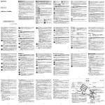
communication to the outside. In statistical computing, the central step usually has two parts: calculation of some
statistics, and evaluations of critical values or factors. In a simplified picture, we can think of four stages.
Import
Statistics
Evaluation
Export
Import and export usually involve a change of the number system: both the internal components and the import/export
components will work with subsets of the rational number, and usually these subsets will not coincide. For example
import and export may interface to ASCII representations where numbers are given to a finite precision, based on
powers of ten, while the internal representation will be binary. If fractions are involved, the missing prime factor 5 in the
internal representation will lead to problems. For example, the decimal number .1 corresponds to the periodic binary
number .0001100110011… No finite binary number will give the exact value. Even if these fractional problems do not
occur, internal and external representation will rarely have coinciding precision: we will have truncation effects. Tests
have to take into account these process stages, implied conversions included. While the truncation problem is wellstudied in numerical calculus, the situation is more complicated in statistical computing, where data is not just numbers.
We may have missing data, out-of-range observations and many other data attributes of real life which go beyond what
is taught in numerical analysis.
Looking at statistical computing from still another point of view, it can be seen as a process transforming (a sequence of)
input data to some statistics which is then evalutated. As a very simple case take a one sample t-test for testing {µ=µ0}
against {µ>µ0}. The result of the statistics is composed of mean, variance and number of observations. Let us assume
that the method of provisional means is taken to calculate the statistics, an iterative algorithm giving the mean and sum of
squared errors of the first i observations for any i. Data are added as they come. Let us assume that the evaluation
calculated the t statistics and looks up the tail probabilities using two approximation algorithms, one for small absolute t,
a different one for sizable or large t.
-2Printed: Wed, 6. Jul, 1994
Numerical Reliability of Data Analysis Systems
Submitted for publication in: Computational Statistics & Data Analyis (ver 1.7)
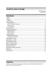
While we are accumulating data, the (mean,ssq) statistics is meandering in R2. After data accumulation, we calculate the
t-statistics and look up the corresponding critical value. Forgetting about the truncation effects, the constraints of our
numerical environment (defined by hardware, compiler and libraries) will lead to overflow as the absolute value of any
numbers gets too large, and to underflow if the values get to small. While overflow usually is a sharp effect, underflow
may occur gradually with decreasing precision until we reach a final underflow limit. These limitations propagate
through our algorithm. So a simplistic carricature of our environment looks like:
SSQ
large t
approx
small t
approx
large t
approx
abs(mean) large: overflow err ??
small t
approx
abs(mean) small: underflow err ??
abs(mean) large: overflow err ??
SSQ large: possible overflow errors
SSQ small: possible underflow errors
SSQ<0: may not occur. Error condition due to numerical errors or incorrect algorithm.
mean
t underflow
possible
t overflow
possible
Even for the one sample t-test, this picture is a simplification. If the statistcs are calculated by the provisional means
algorithm, at data point i+1 the algorithm will depend on the mean of the first i data points, and the difference between
the i.th data point and this provisional mean. So the actual algorithm has at least a three dimensional state space, and is
more complicated than the sketch given here.
From a more abstract point of view, the computing system and the algorithm define a tesselation of the algorithm state
space with soft or sharp boundaries. The actual computation is a random path (driven by the data) in this state space,
with evaluation occuring at the stopping point of this random path. The choice of a testing strategy amounts to the
selection of paths which are particularly revealing. A full testing strategy is:
•
probe each tile of the tesselation.
•
for any boundary, probe on the boundary itself, and probe the boundary transition, that is go from one
tile to near-boundary, to on-boundary, to near-boundary on the tile on the other side.
•
for any vertex, probe on the vertex.
If the state space of our computation is two dimensional, the boundaries are just lines or curve segments. In higher
dimensions, we will meet submanifolds, or strata, of any lower dimension defining our tesselation.
-3Printed: Wed, 6. Jul, 1994
If we have inside knowledge of a system, we can calculate the tesselation exactly – software testing is much easier for
the developer than for the user. If we do not have inside knowledge, the best we can do is gather ideas about possible algorithms and implementations, and try using various resulting tesselation geometries. Using a vendor's documentation is
a source of information, but unfortunately this only adds to the problem. We cannot assume that the documentation is
correct. Hence the vendor documentation only adds one more possible tesselation to take into account.
The number of test situations for a full testing grows rapidly with the number of components involved. As each
component brings its own tesselation, we end up with the product of all numbers of components. This explosion of
complexity is a well-known problem in software engineering. The well-known solution is to use a modular design: if we
can decompose our program into components which are independent, given a well-defined input and producing a welldefined output, we can do a separate component test and the testing complexity is of the order of the sum of the
component complexitites, not the product. In our example, the provisional means algorithm and the t distribution
function could be implemented as separate modules. If we are designing a software system, this can drastically reduce
the complexity of testing.
Unfortunately, a modular design alone is not suficient. To justify a restriction to modular testing, you must be able to
guarantee that the modules are independent. You must design your system using modular algorithms, and you must be
able to guarantee that there is no uncontrolled interaction in the final compiled and linked program. This is where the
choice of the programming language enters. While most languages allow modular programming, only few (like Modula
or Oberon) do actively support it. If modularity is not guaranteed by language, compiler and libraries, uncontrolled
interactions between components of a program could occur. The complexity of testing can only be reduced if all
development tools support modularity.
Intrinsic Conditions
Tesselations may also have be defined by intrinsic conditions. As an example, take linear regression. Sample sizes n=0
and n=1 give exceptional strata. Although these situations usually will be detected by the user, a (commercial) data
analysis system should have precautions to handle these exceptions. Constant response, or more generally any response
uncorrelated to the regressors, could be considered exceptional situations defining additional strata for the tesselation.
Although these exceptional situations can be handled consistently in the usual regression context, in some
implementations they may be treated as special cases, thus requiring additional test cases. A third set of strata comes
from rank deficiencies, related to collinearity in the regressors. Even in theory these situations need special
consideration. So collinearities are obvious candidates for test cases.
More complex strata arise from inherent instabilities of the regression problem. These instabilities are based in the matter
of the subject, and do not depend on any particular algorith or implementation: In theory, estimation in a linear model can
be done exactly by solving the normal equations (at least if we have full rank, no missing data, no censoring etc.). This
amounts to solving a linear equation of the form
X'Xb=X'Y
with solution b*
for a parameter vector b, where X is the design matrix and Y is the vector of observed responses. On any finite system,
we can have only a finite representation of our data. What we can solve is an approximation
(X'X+E)b=X'Y+e
with solution b~
with some initial error matrix E on the left hand side, and an initial error vector e on the right. These errors occur before
any calculation and are an unavoidable errror on a finite system. It is still possible to give bounds on the relative error
||b*-b~||/||b*||. These bounds usually have the form ||b*-b~||/||b*|| ≤ ||X'X|| ||(X'X)-|| ⋅…, where the product of the matrix
norms ||X'X|| ||(X'X)-|| is controlling the error bound. This number is known as the condition number in numerical
literature, and regression problems are well-known to be potentially ill-conditioned. Even when the problem is very
-4Printed: Wed, 6. Jul, 1994
small, it may be ill-conditioned. To illustrate this, here is an example from numerical text-book literature (after
Vandergraft 1983). Take a simple linear regression model Y=a+bX+err for these data
X:
Y:
10.0
1
10.1
1.20
10.2
1.25
10.3
1.267
10.4
1.268
10.5
1.276
In theory, the solution can be derived from the normal equations which can be very easily found to be
6b0 + 61.5b1 = 7.261
61.5b0 + 630.55b1 = 74.5053
giving a regression Y= -3.478 + 0.457 X. To illustrate the risk that comes with ill-conditioning, we change the second
line of the normal equations by rounding it to four significant digits, giving
6b0 + 61.5b1 = 7.261
61.5b0 + 630.6b1 = 74.51
and we get a regression Y= -2.651 + 0.377 X. A relative change of order 10-4 in the coefficients has caused a relative
change or order 1 in the regression coefficients.
While we use normal equations for theory we will use more efficient or more stable approaches for computation.
However the sensitivity to ill-conditioning is already present in the exact solution for theoretical situation. It will affect
any implementation. From this we know that any (finite) algorithm is bound to become affected if the problem gets illconditioned. So we must test for behaviour in ill-conditioned situations.
Apart from aspects of statistical computing, ill-conditioning puts a challenge to the other one of the these twin disciplines, to computational statistics. If statistical computing is doing its work, computational statistics has still to supply
statistical methods which are adequate in ill-conditioned situations, even if the data we get are discretized to a certain precision. A relative change of the date of order 10-3 in our example can easily produce a change of order in the coefficients
of the normal equation, leading to the drastic effect illustrated above. The error which comes from truncation or rounding
of input data in this example is in the same order of magnitude as the estimated standard error of the coefficients. But in
computational statistics literature, you will rarely find hints even how to do a valid regression for realistic (truncated,
rounded) data.
Computer Arithmetics and Numerical Reliability
Real number arithmetics is the heart of the tests at hand, and the interplay between hardware, compiler and algorithm can
be illustrated here. In a computer, we do not have real numbers, but only a finite discrete approximation. Computer reals
often are stored in an exponential representation, that is as a pair (m,p) to represent a real number x=m*10p, where the
mantissa m is a fixed point number and the exponent p an integer. Additional normalization conditions are used to save
space and time, for instance requiring a choice of p so that the most significant bit of m is one. This representation has
various pitfalls (for a discussion from the point of view of the seventies, see, e.g. Sterbenz 1974; for a more recent
discussion see Goldberg 1991). For example to subtract two numbers, both numbers are aligned to have same power,
then a fixed point subtraction on the mantissas is performed, and finally the result is re-normalized. For numbers of
nearly equal size, the results consists of the last few digits of the mantissas, plus additional stray bits coming from the
various conversions. You can not generally assume that x-y=0 if and only if x=y. Rounding is another weak point: in
old systems, the rounding direction used not to be adjusted with arithmetic operators or functions. As a consequence,
you could not even assume that 3*(1/3)=1.
You can get an impression of the round-off behaviour of your preferred system by checking the following expressions:
INT(2.6*7 -0.2)
2-INT(EXP(LN(SQRT(2)*SQRT(2))))
INT(3-EXP(LN(SQRT(2)*SQRT(2))))
should be: 18
should be: 0
should be: 1
where LN is the natural logarithm and INT is an integer function. Since these arithmetic expressions have integer results,
you in theory should get the same result for any real to integer conversion your system can provide. For example, INT
can be the "round to zero" truncation converting decimal numbers to integers by throwing away the digits after the
-5Printed: Wed, 6. Jul, 1994
decimal point. Or it can be a floor function giving the largest integer value not exceeding a number, or any other real to
integer conversion.
While in theory you can expect exact results, in practive the best you can hope for is to be able to control rounding
directions. You cannot control the internal arithmetics, and a typical result may look like the following table calculated by
S-PLUS, using four real to integer conversions (trunc, round, floor, ceiling). The real number returned by S-Plus is
shown in the last column
INT(2.6*7 -0.2)
2-INT(EXP(LN(SQRT(2)*SQRT(2))))
INT(3-EXP(LN(SQRT(2)*SQRT(2))))
true
18
0
1
trunc
18
1
1
round
18
0
1
floor
18
1
1
ceiling
18
0
2
real
18
4.44e-16
1
The current state of the art is given by the IEEE standard 754 for binary floating-point arithmetic. This standard is still
based on an exponential representation. But it has more flexible normalization conditions, to allow for more significant
digits in the mantissa if the exponent becomes small. In an IEEE arithmetic, you can guarantee that x-y=0 if and only if
x=y. Or that (x-y)+y evaluates to x, even if an underflow occurs in the calculation of (x-y), while a historical "fade to
zero" arithmetics might evaluate this to y. Various rounding directions are defined so that F-1F(x)=x for a large class of
functions. Moreover, the IEEE standard reserves bits to denote special cases: infinities and non-numerical values (not a
number: NaN). So you can have 1/0 giving INF, -1/0 giving -INF, 2*INF giving INF, -INF/INF giving NaN etc.
IEEE is supported in hardware in most modern chips, including the 80xxx line of INTEL and the MOTOROLA 68xxx
line. If the hardware does not support IEEE arithmetics, the compiler and its libraries may still support it. This means
that the compiler has to add additional checks and conversions to map the basic arithmetic supported to an IEEE
arithmetic. This will imply a computational overhead – the price you have to pay for the initial choice of hardware. If
neither the hardware nor the compiler do support a high quality arithmetic, the programmer can emulate it on the
application level. This puts a burden on the programmer which could be easier carried by other instances – the
programmer has to pay for the choice of hardware and compiler. Since in general more optimizing tools are available for
compiler construction and their libraries than are available for the application programmer, this may imply an additional
performance loss over a compiler-based solution.
We are interested in the application side, not in the developer's side. So we have to ask for the reliability returned for the
user. It is not our point to ask how the implementer achieved this reliability. But we should not set up unrealistic goals.
Understanding some of the background may help to judge what can be achieved, and may clarify some of symptoms we
may see in case of a failure. For example, we must accept that the available precision is limited. Let us assume, for
example that the input contains a string which is beyond limits. If the string is non-numeric, the system should note this
and take adequate action. All systems under test do this in their latest version we have seen. If the string is numeric, but
out of range for the system (too large or too small), an appropriate error message should be given, and the value should
be discarded from further calculations. A IEEE arithmetic would return a NaN value. The string could not be converted
to a number. In an IEEE environment, it is sufficient to check whether the number read in is of class NaN, and to take
the appropriate action. We have to accept this sort of behaviour. In an IEEE-system, if no appropriate action is taken on
the program level, the NaN value will propagate consistently and we will have a plausible side exit. In a non-IEEE
environment, additional checks have must be added by the programmer to make sure that the number read in actually
corresponds to a number represented by the input string. If this check is done, the behaviour is equivalent to that in an
IEEE environment. If this check is omitted, we run into an arbitrary solution – the worst of all possible cases. As a
matter of fact, two of the systems under test showed these symptoms.
Both the historical arithmetics as well as more recent IEEE-based systems allow for different sizes of the mantissa. In the
-6Printed: Wed, 6. Jul, 1994
jargon of the trade, by misuse of language, this is called precision. All numerical data in Wilkinson's test can be read in
with traditional double precision arithmetic. So in principle all systems had the chance not only to do a proper diagnostic,
but also to recover automatically.
Poor programming may be hidden by a sufficient basic precision. As an example, take the calculation of the variance.
One of the worst things to do is to use the representation s2=(1/n-1) (∑xi2 - n x2). Since ∑xi2 and n x2 differ only by
the order of the variance of ∑xi, we run into the problem of subtractive cancellation: we get only a small number of
trailing bits of the binary representation of the mantissa if the variance is small compared to the mean. A better solution is
to take the method of provisional means, an iterative algorithm giving the mean and sum of squared errors of the first i
observations for any i.The poor algorithm for the variance based on s2=(1/n-1) (∑xi2 - n x2) will break down at a
precision of 4 digits on a data set where Var(Xi) ≈ 0.01 E(Xi). It will have acceptable performance when more digits of
precision are used. Adherence to the IEEE standard may add to acceptable performance even of poor algorithms. Many
systems tested here are implemented in a double precision (8 bytes) arithmetic, or even in an extended IEEE system with
10 bytes of basic precision.
Well-Known Problems
Numerical precision has always been a concern to the statistical community (Francis et al. 1975, Molenaar 1989, Teitel
1981). Looking at fundamental works like Fisher (1950), you will find two issues of concern:
•
Truncation or rounding of input data
•
Number of significant digits.
For truncation or rounding effects, the solution of the early years of this century was to split values meeting the
truncating or rounding boundaries to adjacent cells of the discretization. To make efficient use of significant digits, a
pragmatic offset and scale factor would be used. So for example, to calculate mean and variance of LITTLEi, i=0..9:
0.99999991, 0.99999992, 0.99999993, 0.99999994, 0.99999995, 0.99999996, 0.99999997, 0.99999998 0.99999999,
the calculation would be done on LITTLEi': LITTLEi=0.99999990+0.00000001*LITTLEi', that is on LITTLEi',
i=1..9:
1, 2, 3, 4, 5, 6, 7, 8, 9
and then transformed back to the LITTLE scale. This would allow effective use of the available basic precision.
For a by now classical survey on problems and methods of statistical computing, see Thisted's monograph (1988).
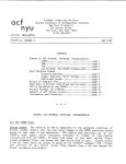
Bad numerical conditions for matrices is a well-known potential problem, in particular in regression. But it took a long
time (until about 1970) to recognize the practical importance of this problem. The Longley data played a crucial role in
providing this awareness. The Longley data is a small data set with strong internal correlation and large coefficients of
variation, making regression delicate.
-7Printed: Wed, 6. Jul, 1994
GNP_Deflator
83.0
88.5
88.2
89.5
96.2
98.1
99.0
100.0
101.2
104.6
108.4
110.8
112.6
114.2
115.7
116.9
GNP
234289
259426
258054
284599
328975
346999
365385
363112
397469
419180
442769
444546
482704
502601
518173
554894
Unemployed
2356
2325
3682
3351
2099
1932
1870
3578
2904
2822
2936
4681
3813
3931
4806
4007
Armed_Forces
1590
1456
1616
1650
3099
3594
3547
3350
3048
2857
2798
2637
2552
2514
2572
2827
Population
107608
108632
109773
110929
112075
113270
115094
116219
117388
118734
120445
121950
123366
125368
127852
130081
Year
1947
1948
1949
1950
1951
1952
1953
1954
1955
1956
1957
1958
1959
1960
1961
1962
Employed
60323
61122
60171
61187
63221
63639
64989
63761
66019
67857
68169
66513
68655
69564
69331
70551
Longley Data. US population data [thousands]. Dependend variable is "Employed". Source: Longley (1967)
The Numerical Reliability Project
This paper has been motivated by an extensive project on testing numerical reliability, carried out in 1990-1993. This
project has revealed a surprising amount of errors and deficiencies in many systems, calling for a broader discussion of
the problems at hand. For a detailed report on the project, see (Sawitzki 1994).
The general ideas laid out so far give an outline of how a test for numerical reliability could be designed. In any particular
application area, this general test strategy may be used to specify particular test exercises. These tests must be evaluated
with proper judgement. Instead of requiring utmost precision, we should ask for reliability. The analysis systems should
recognize their limits and give clear indications if these limits are reached or exceeded. If a system behaves reliably, this
must be respected, even if some calculations cannot be performed. On the other side, if a system fails to detect its
limitations, this is a severe failure.
The tests reported in (Sawitzki 1994) concentrated on regression, a particularly well-studied area in statistical computing.
Following the ideas laid out above, the tesselation of the problem space given by different algorithmic regimes defines a
test strategy. This includes tesselations as defined by the available numerics, but also tiles defined by statistical limiting
cases, like constant regression or other degenerate cases.
For a stringent test, using a set of test exercises with fixed numbers is not adequate. Different software products will
have limits in different regions. Data sets designed to test the limits of one product may be well in scope for another one.
Instead of using fixed test data sets, the data used for evaluation should be generated specifically for each system,
respecting the relative system boundaries. Strategies to do so are discussed in Velleman and Ypelaar (JASA 75).
But for every-day situations with not too extreme data however it is possible to provide fixed test data sets. A small but
effective set of test data is suggested by Leland Wilkinson in "Statistics Quiz" (1985). The basic data set is
-8Printed: Wed, 6. Jul, 1994
Labels
ONE
TWO
THREE
FOUR
FIVE
SIX
SEVEN
EIGHT
NINE
X ZEROMISS
1
0
•
2
0
•
3
0
•
4
0
•
5
0
•
6
0
•
7
0
•
8
0
•
9
0
•
BIG
99999991
99999992
99999993
99999994
99999995
99999996
99999997
99999998
99999999
LITTLE
0.99999991
0.99999992
0.99999993
0.99999994
0.99999995
0.99999996
0.99999997
0.99999998
0.99999999
HUGE
1.0E+12
2.0E+12
3.0E+12
4.0E+12
5.0E+12
6.0E+12
7.0E+12
8.0E+12
9.0E+12
TINY
1.0E-12
2.0E-12
3.0E-12
4.0E-12
5.0E-12
6.0E-12
7.0E-12
8.0E-12
9.0E-12
ROUND
0.5
1.5
2.5
3.5
4.5
5.5
6.5
7.5
8.5
As Wilkinson points out, these are not unreasonable numbers:
"For example, the values of BIG are less than the U.S. population. HUGE has values in the same order as the
magnitude of the U.S. deficit2. TINY is comparable to many measurements in engineering and physics."
This data set is extended by the powers X1=X1,...X9=X9. The test tasks are various correlations and regressions on
this data set. Trying to solve these tasks in a naive way, without some knowledge in statistical computing, would lead to
a series of problems, like treatment of missing data, overflow and underflow, and ill-conditioned matrices. The detailed
tasks are given in Wilkinson (1985).
Wilkinson's exercises are not meant to be realistic examples. A real data set will rarely show a concentration of problems
like Wilkinson's exercises. The exercises are deliberately designed to check for well-known problems in statistical
computing, and to reveal deficiencies in statistical programs. The "Statistics Quiz" does not test applicability for a certain
purpose, or sophisticated issues of a data analysis system. All problems checked by this test have well-known solutions.
We have already mentioned some techniques used in earlier days to make efficient use of the available arithmetics. None
of the numerics involved in Wilkinson's basic data would have been a problem in the beginning of this century.
Wilkinson's exercises cover a fraction of the testing strategy laid out so far. From a systematic point of view, this is not
satisfactory. But from a pragmatic point of view, a stringent test is only worth the effort after entry level tests are passed.
Wilkinson's test has been circulated for many years now, and is well known in the software industry. It does not pose
any exceptional or unusual problems. By all means, it qualifies as an entry level test. Our test exercises lean on
Wilkinson's test suite. The results given in the report (Sawitzki 1994) show serious deficiencies in most systems, even
when confronted whith these entry level tests.
Test Exercises
Leland Wilkinson (1985) suggested a series of tests covering various areas of statistics. We restrict ourselves to the
elementary manipulations of real numbers, missing data, and regression. In Wilkinson (1985), these are problems
II.A–II.F, III.A–III.C, and IV.A–IV.D. For easier reference, we will keep these labels.
The elementary tests are
II.A Print ROUND with only one digit.
II.B Plot HUGE against TINY in a scatterplot.
II.C Compute basic statistics on all variables.
2The data set was published in 1985.
-9Printed: Wed, 6. Jul, 1994
II.D Compute the correlation matrix on all the variables.
II.E Tabulate X against X, using BIG as a case weight.
II.F Regress BIG on X
We should assume that commercial software is properly tested. Any decent testing strategy includes test data sets,
covering what has been discussed above. If this geometry of the problem is well-understood, a usual test strategy is to
select a series of test cases stepping from the applicable range to near boundary, to the boundary, exceeding and then
moving far out. Moving this way may lead to another standard test strategy: checking the scale behaviour of the
software. The variables BIG, LITTLE, HUGE, TINY allow to check scaling properties.
If we accept the data in Wilkinson's data set as feasible numbers, none of these test should imply a problem. All of these
test should fall into the basic tile of "no problem" cases. These task imply a test of the import/export component of the
system. This is an often neglected point, noted only rarely (one exception being Eddy and Cox (1991): "The importance
of this feature can be inferred from the fact that there are commercial programs which provide only this capability").
Surprisingly, some of the commercial systems, such as ISP or some versions of GLIM, cannot even read the data table
of Wilkinson's test without problems. For example, GLIM (Version 3.77 upd 2 on HP9000/850) could not read in the
data set. Without any warning or notice, GLIM interpreted them as
X
1
2
3
4
5
6
7
8
9
BIG
99999992
99999992
99999992
99999992
99999992
100000000
100000000
100000000
100000000
LITTLE
1.000
1.000
1.000
1.000
1.000
1.000
1.000
1.000
1.000
As we have stated above, it is unrealistic to expect all systems to be able to solve any problem. Any system will have its
limitations, and these must be repected. But it is not acceptable that a system meets its boudaries without noticing.
Giving no warning and no notice, and procceding with the computation based on an incorrect data representation is an
example of what has been labeled the Ultimate Failure: running into an arbitrary solution.
The solutions should be for the summary (task II.C)
X
ZERO
Means
5.0 0
StdDev
s
0
Variance 7.5 0
MISS
•
•
•
BIG
9.9999995e+7
s
7.5
LITTLE
0.99999995
s*1e-8
7.5e-16
HUGE
5.0e+12
s*1e+12
7.5e+24
TINY
5.0e-12
s*1e-12
7.5e-24
ROUND
4.5
s
7.5
where s is 2.73861278752583057… to some precision.
The correlation matrix (task II.D) should be for any type (parametric or non-parametric) of correlation:
X
ZERO
MISS
BIG
LITTLE
HUGE
TINY
ROUND
X
1
1
1
1
1
1
1
1
ZERO
MISS
BIG
LITTLE
HUGE
TINY
ROUND
•
•
•
•
•
•
•
•
•
•
•
•
•
1
1
1
1
1
1
1
1
1
1
1
1
1
1
1
The regression results should be
BIG
=
(task II.F)
99999990 + 1 * X
- 10 Printed: Wed, 6. Jul, 1994
Missing data are an ubiquitous feature of real data sets. This situation needs special consideration. The handling of
missing data is tested in three tasks.
III.A Generate a new variable TEST using the transformation
IF MISS=3 THEN TEST=1 ELSE TEST=2.
III.B Transform MISS using IF MISS=<missing> THEN MISS=MISS+1.
III.C Tabulate MISS against ZERO.
Regression is inspected using the tasks
IV.A Regress X on (X2, X3, … X9)
This is a perfect regression, but prone to stress the arithmetic conditions. In a stringent test series, a sequence of matrices
with increasing ill-conditioning would be used instead. IV.A is a pragmatic test, posing a regression problem in a form
which is quite usual for user from physics, chemistry or other sciences heading for a polynomial approximation.
Regressing X=X1 on X2…X9 addresses the problem seen in the Longley data. While most of these tasks have
straightforward correct solutions, the polynomial regression (IV.A) is bound to push the arithmetics to its limits. There
will be differences in the coefficients calculated, and these should be judged with proper discretion. The regression, not
the coefficient, is the aim of the calculation. Besides the residual sum of square, as reported by the package, we give the
integrated square error over the interval [0…10] as additional measure of goodness of the fit. Since IV. A allows a
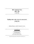
perfect fit residuals should be zero. For the solution given below, the integrated square error is 0.0393.
Polynomial fit of degree 9 without linear term, to a line (Task IV.A).
Residual sum of squares < 2e-20.
10
(f(x) - x )2dx = 0.0392702.
Integrated square error
0
For this regression test, the results should be
(task IV.A)
X
=
0.353486
+
+
+
+
-
1.14234 * X2
0.704945 * X3
0.262353 * X4
0.061635 * X5
0.00920536 * X6
0.000847477 * X7
0.000043835 * X8
9.74112*(10^-7) * X9
IV.B Regress X on X
Again a perfect regression, testing the intrinsic stratum of |correlation|=1. The correct solution is
(task IV.B)
X
=
0 + 1 * X
- 11 Printed: Wed, 6. Jul, 1994
IV.C Regress X on (BIG,LITTLE)
A collinearity of the most simple kind: linear dependence between two regressors . Any solution giving a clear diagnostic
should be considered correct, as well as any solution giving the correct fit.
(task IV.C)
X
=X(BIG,LITTLE)
is a singular model because BIG and LITTLE are linearly dependent.
IV.D Regress ZERO in X
This is testing for the exceptional stratum where the regressor is constant. with the obvious solution
(task IV.D)
ZERO
=
0*X + 0.
We added two tasks:
(IV.E) regress X on X2…X9, but using the regressors in a permuted order.
As we have already discussed above, regression may lead to ill-conditioned problems. Thus solutions may be inherently
unstable. For reasons of time or space economy, regression may be solved by an iterative method, like the SWEEP
operator (Beaton 1964, Goodnight 1979), a space conserving variant of the Gauss-Jordan elimination method. The
SWEEP operator usually is used in an iteration which adds one regressor at a time. But if any iterative method is used,
subsequent iteration steps may lead to a magnification of errors, particularly in an ill-conditioned situation. The result
will then depend strongly on the order of iteration steps. For the SWEEP operator, this is the order in which the
variables are entered. Test IV.E tests for this order dependence. The solution should be the same as in IV.A.
There may be good reasons to chose the SWEEP operator in certain implementations. For example this choice has been
taken in Data Desk in order to allow interactive addition or removal of variables in a regression model. But the risk is
high, as is illustrated by the following results returned by Data Desk for polynomial regression task IV.A/IV.E for the
same data set, using the original and a permuted order of regressors.
Dependent variable is:
X1
No Selector
R squared = 100.0%
R squared (adjusted) = 100.0%
s = 0.0018 with 9 - 8 = 1 degrees of freedom
Source
Sum of Squares
df
Regression
Residual
60.0000
0.000003
7
1
Mean Square
F-ratio
8.57143
0.000003
2798812
Variable
Coefficient
s.e. of Coeff
t-ratio
Constant
X2
X3
X4
X5
X6
X7
X8
X9
0.385710
1.01212
-0.534297
0.163478
-0.030038
3.26631e-3
-1.93556e-4
4.81330e-6
0
0.0112
0.0334
0.0358
0.0164
0.0040
0.0005
0.0000
0.0000
0
34.5
30.3
-14.9
9.95
-7.55
6.16
-5.26
4.64
•
- 12 Printed: Wed, 6. Jul, 1994
prob
0.0184
0.0210
0.0426
0.0637
0.0838
0.1024
0.1196
0.1352
•
Dependent variable is:
X1
No Selector
R squared = 100.0%
R squared (adjusted) = 100.0%
s = 0.0023 with 9 - 8 = 1 degrees of freedom
Source
Sum of Squares
df
Regression
Residual
60.0000
0.000005
7
1
Mean Square
F-ratio
8.57143
0.000005
1671633
Variable
Coefficient
s.e. of Coeff
t-ratio
Constant
X8
X9
X4
X5
X2
X3
X6
X7
0.395833
-6.65266e-6
0.00000e+0
0.133437
-0.020527
0.971796
-0.481949
1.49418e-3
0
0.0124
0.0000
0.0000
0.0142
0.0029
0.0342
0.0343
0.0003
0
31.8
-4.44
4.02
9.42
-7.17
28.4
-14.1
5.87
•
prob
0.0200
0.1410
0.1554
0.0674
0.0882
0.0224
0.0452
0.1074
•
Another task we added was:
(IV.F)
Regress X'=X/3 on (X'2,X'2,…X' 9).
This was added to check for number representation effects. Using the example of the Longley data, Simon and Lesage
(1988) have pointed out that going from integer data to data of similar structure, but real values, can drastically change
the findings. This is what is to be expected for ill-conditioned problems, if the integer/real conversion leads to any
internal rounding or truncation.
These tasks do not cover the full program laid out above. In particular, they do not include real boundary testing for a
given system. All test exercises fall in a range which could be easily handled, given the arithmetic systems and software
technologies which are widely abvailable. In this sense, the test exercises can be considered an entry level test. Systems
passing this test may be worth a more thorough inspection. The test has been applied to several common systems. The
results are presented in a separate paper (Sawitzki 1994).
- 13 Printed: Wed, 6. Jul, 1994
Literature
IEEE Std 754-1985. IEEE Standard for Binary floating-Point Arithmetic (IEEE, Inc. New York, 1985).
Beaton, A.E., The Use of Special Matrix Operators in Statistical Calculus (Ed.D. thesis, Harvard University, 1964.
Reprinted as Research Bulleting 64-51, Educational Testing Service, Princeton, New Jersey).
Chambers, J., Computational Methods for Data Analysis (Wiley, NewYork, 1977).
Eddy, W.F. and L.H. Cox, The Quality of Statistical Software: Controversy in the Statistical Software Industry,
Chance 4 (1991) 12-18.
Fisher, R., Statistical Methods for Research Workers (Oliver and Boyd, Edinburgh, 195011).
Francis, I. and R.M. Heiberger, The Evaluation of Statistical Program Packages – The Beginning. In: J.D.W.Frane
(Ed.), Proceedings of Computer Science and Statistics: 8th Annual Symposium on the Interface 1975, 106-109.
Francis, I. , R.M. Heiberger and P.F. Velleman, Criteria and Considerations in the Evaluation of Statistical Program
Packages. The American Statistician (1975) 52-56.
Goldberg, D., What Every Computer Scientist Should Know About Floatin-Point Arithmetic, ACM Computing Survey
23 (1991) 5-.
Goodnight, J.H., A Tutorial on the SWEEP Operator, The American Statistician 33 (1979) 149-158
Longley, J.W., An Appraisal of Least-Squares for the Electronic Computer from the Point of View of the User, Journal
of the American Statistical Association 62 (1967) 819-841.
Molenaar, I.W., Producing, Purchasing and Evaluating Statistical Scientific Software: Intellectual and Commercial
Challenges, Statistical Software Newsletter 15 (1989) 45-48
Sawitzki, G., Report on the Numerical Reliability of Data Analysis Systems, Computational Statistics and Data
Analysis (SSN) 18(2) (Sep. 1994).
Sterbenz, P.H., Floating-Point Computation, (NJ:Prentice-Hall, Englewood Cliffs, 1974).
Simon, S.D. and J.P. Lesage, Benchmarking Numerical Accuracy of Statistical Algorithms, Computational Statistics
and Data Analysis 7 (1988) 197-209.
Teitel, R.F., Volume Testing of Statistical/Database Software. In: W.F. Eddy (Ed.) Proceedings of Computer Science
and Statistics. 13th Annual Symposium on the Interface 1981, 113-115
Thisted, R., Elements of Statistical Computing, (Chapman and Hall, New York, 1988).
Wilkinson, L., Statistics Quiz, (Systat, Evanston, 1985).
- 14 Printed: Wed, 6. Jul, 1994
Vandergraft, J.S., Introduction to Numerical Computations, (Academic Press, New York, 1983).
Velleman, P. and M.A. Ypelaar, Constructing Regressions with Controlled Features: A Method for Probing Regression
Performance, Journal of the American Statistical Association 75 (1980) 834-844.
- 15 Printed: Wed, 6. Jul, 1994
Report on the Numerical Reliability of Data Analysis Systems3
Günther Sawitzki
StatLab Heidelberg
Im Neuenheimer Feld 294
6900 Heidelberg
For all contributors: please double-check again: are input/output format overflows handled correctly ?
Please send in last-minute corrections and contributions to G. Sawitzki, StatLab Heidelberg
([email protected]–heidelberg.de)
Summary
From 1990 to 1993, a series of test on numerical reliability of data analysis systems has been carried out. The tests are
based on L.Wilkinson's "Statistics Quiz". Systems under test included BMDP, Data Desk, Excel, GLIM, ISP, SAS,
SPSS, S-PLUS,STATGRAPHICS. The results show considerable problems even in basic features of well-known
systems. For all our test exercises, the computational solutions are well known. The omissions and failures observed
here give some suspicions of what happens in less well-understood problem areas of computational statistics. We cannot
take results of data analysis systems at face value, but have to submit them to a large amount of informed inspection.
Quality awareness still needs improvement.
Results by product: (In alphabetical order)
This is a report on basic numerical reliability of data analysis systems. The test reported here have been carried out by
members of the working group Computational Statistics of the International Biometrical Society (DR) and the working
group "Statistical Analysis Systems" of the GMDS 1990-1993, based on Leland Wilkinson's "Statistical Quiz".
We started the investigations on numerical reliability at the Reisensburg meeting 1990. We restricted our attention to
Wilkinson's "Statistical Quiz" at the meeting of the Biometrical society in Hamburg 1991. We did not attempt a market
survey, but concentrated on those product which are in practical use in our working groups. A first round of results was
collected and discussed with the vendors represented at the Reisensburg meeting 1991. A second round was collected
and discussed 1992, a final round in 1993. The vendor reaction ranged anywhere between cooperative concern and rude
comments.
By now, we do think that the software developers had enough time to respond and a publication is not unfair.
We give a summary of the results for
BMDP
Data Desk
Excel
GLIM
ISP
SAS
SPSS
S-PLUS
STATGRAPHICS
Versions and implementations tested are listed in the appendix. We deliberately have decided not to run for the most
recent version which may be announced or on the market. So far, software vendors rarely take their responsibility and
usually do not provide users with free bug fixes and upgrades. In this situation, looking at the software that is actually
used is more important than looking at what is advertised.
BMDP
3This report was presented at the 25th Workshop on Statistical Computing, Schloß Reisensburg 1984. Contributors:
G. Antes (Univ. Freiburg), M. Bismarck (M.-Luther-Universität Halle-Wittenberg), P. Dirschedl (Univ. München), M. Höllbacher (Univ.
Erlangen-Nürnberg), A. Hörmann (gsf/medis Neuherberg), H.-P. Höschel (SAS Institute Heidelberg), T. Huber (Datavision AG, Klosters), A.
Krause (Univ. Basel), M. Nagel (Zentrum f. Epidemiologie u. Gesundheitsforschung Berlin/Zwickau), G. Nehmiz (Dr. Karl Thomae GmbH,
Biberach), C. Ortseifen (Univ. Heidelberg), R. Ostermann (Univ.-GH–Siegen), R. Roßner (Univ. Freiburg), R. Roth (gsf/medis Neuherberg),
W. Schollenberger (SAS Institute Heidelberg), J. Schulte Mönting (Univ. Freiburg), W. Vach (Univ. Freiburg), L. Wilkinson (Systat Inc,).
- 16 Printed: Wed, 6. Jul, 1994
BMDP has been setting the standards for statistical computing for a long time. Being one of the first packages, it
inevitably had its problems with a heavy FORTRAN heritage, and it is known that BMDP is working for an
improvement. We tested the 1990 workstation version on a SUN. The first attempts using BMDP1R failed on our data
set, in particular on the polynomial regression task (task IV) using any allowed tolerance level in the range between 1.0
or 0.001. Only when exceeding this tolerance level, e.g. by typing in a tolerance level of 0.0001, a hint to BMPD9R was
returned.
With BMDP9R and default settings, the problem was not solved. An appropriate warning was returned:
NOTE THAT 5 VARIABLES HAVE BEEN OMITTED BECAUSE OF LOW TOLERANCE.
After a long series of attempts it turned out that BMPD would accept
tolerance=0.000 000 000 000 1.
The BMDP output would show a report
TOLERANCE FOR MATRIX INVERSION........0.0000000
The regression is calculated and commented by
***
NOTE
*** THE DEPENDENT VARIABLE IS A LINEAR COMBINATION OR A
NEAR LINEAR COMBINATION OF THE INDEPENT VARIABLE.
THE PROGRAM WILL SKIP TO THE NEXT PROBLEM.
Polynomial fit of degree 9 without linear term, to a line (Task IV.A).
Polynomials fitted by BMDP9R (for details, see text). Calculation aborted by BMDP, no residual sum of squares
reported by BMDP. Integrated square error=0.038924.
Regressing X on X (task IV.B) lead to a system error within BMDP. The program crashed in the middle of an error
message. After making a copy of X and regressing on this, a proper result was returned by BMDP.
Regressing X on BIG and LITTLE (task IV.C) lead to completely misleading results in BMDP1R and BMDP9R.
Regressing X on ZERO was solved correctly.
Data Desk
The summary statistics for LITTLE returned a standard deviation of 3E-8 and a variance of 0, standard deviation and
variance for TINY were 0 (task II.C).
Data Desk (version 4.1.1) could handle the original perfect polynomial regression task (IV.A) in so far as the coefficients
returned gave an acceptable fit. But if the regressors were entered in a different order, a different result would be
returned. Although the residual sum of square are rather small when calculated using the internal representation of Data
Desk, the polynomial printed out is rather far off in the second case. There seems to be a discrepancy between the
internal data and the regressing reported to the user. Since in Data Desk the user does not have access to the internal
information, this problem can be critical.
- 17 Printed: Wed, 6. Jul, 1994
Polynomial fit of degree 9 without linear term, to a line (Task IV.A).
Two polynomials fitted by Data Desk (for details, see text). Integrated square error=0.0486 resp.42475.2.
For the collinear model (IV.C), all weight was given to the first regressor entered; no warning was issued.
The degenerate regressions (IV.B and IV.C) were passed without problems.
EXCEL
Microsoft EXCEL, and other spreadsheet programs, claim to be systems for data analysis. They should be taken by their
word and included in this test. EXCEL 4.0 failed to calculate even the summary statistics (task II.C). It returned errors
starting at the first significant digit. It was not even stable enough to produce the same standard deviation for X and
ROUND using the standard EXCEL functions AVERAGE(), VAR() and STDEV().
mean
var
stddev
X
5
7.5
2.73861279
BIG
99999995
6
2.449489743
LITTLE
0.99999995
8.88178E-16
2.98023E-08
HUGE
5E+12
7.5E+24
2.73861E+12
TINY
5E-12
7.5E-24
2.73861E-12
ROUND
4.5
7.5
2.738612788
These results are most surprising, particularly on the Macintosh. The Macintosh operation system, going beyond more
classical systems, supports a full extended precision IEEE arithmetics as part of the operating system. Using these
operating system facilities, even the most crude algorithm would give a correct value for variance and standard deviation
in our test.
Although EXCEL did not manage to calculate the variance correctly, they got correct results for all the correlations (task
II.D), using CORREL(). EXCEL gave satisfactory results for the polynomial regression problem (task IV.A) using the
"Regression" analysis tool packed with EXCEL (residual sum of square: 1.093E-13; integrated square error=0.049).
EXCEL failed to diagnose the singularity when regressing X on BIG and LITTLE (task IV.C)and gave a regression
Intercept
BIG
LITTLE
Coefficients
Standard Error
t Statistic
P-value
-125829115
1.258291259
0
11828363.26
0.236567273
19379590.84
-10.637914
5.31895746
0
5.3396E-06
0.00071193
1
GLIM
GLIM is made for generalized linear models. So it should be capable to handle easy things like estimating in linear
models, setting the error probability function to normal, and using identity as a link function.
- 18 Printed: Wed, 6. Jul, 1994
GLIM (Version 3.77 upd 2 on HP9000/850) could not read in the data set. Without any warning or notice, GLIM
interpreted them as incorrectly. We have been informed by NAG, the distributor of GLIM, that this problem would not
occcur with the double precision version of GLIM on VMS of on a Cray. Obviously GLIM has no sufficient error
checking to detect input problems if values are our of scope for a given version.
Default plots did not show sufficient resolution to represent the data set. GLIM had problems calculating mean values
and standard deviations (task II.C) for BIG and LITTLE. Besides the input problem seen above, more numerical
problems seem to affect GLIM.
Variable
mean
variance
SE
_______________________________________________________
X
5.000
7.500
0.9129
ZERO
0
0
0
BIG
99999992
17.78
1.405
1.283e-15
1.194e-08
LITT
1.000
HUGE
5.000e+12
7.500e+24
9.129e+11
TINY
5.000e-12
7.500e-24
9.129e-13
ROUN
4.500
7.500
0.9129
Not all simple regression problems could be handled by GLIM. Taking into account the input problem, regressing BIG
on X (task II.F) gave wrong results
Intercept 99999992.
Slope
1.333 (s.e. 0.2910) instead of 1.
The polynomial regression test (task IV.A) was satisfactory for low powers, but gave wrong results for powers above 6,
and drastic errors for powers 8,9. For regression of X on BIG and LITTLE (task IV.C), the singularity could not be
identified as a consequence of the error in reading the data.
GLIM Regression evaluations:
Variables
| intercept
slope
| if incorrect: should be
| (s.e.)
(s.e.)
| intercept slope (s.e.=0)
______________________________________________________________
ZERO on X | 0
0
| | (0)
(0)
X on X
| 0
| (0)
BIG on X
| 99999992
| (1.637)
X on BIG
| -56249992
| (12274756)
X on LITT
| -63882468
| (15879222)
1
(0)
| -
-
1.333
(0.2910)
| 99999990
|
1
0.5625
(0.1227)
| -99999990
|
1
63882476 | 0.99999990 0.00000001
(15879223) |
ISP
The standard single precision version of ISP had so many problems that we discarded it from the test. The situation
however is other than for GLIM, since ISP is available in double precision version DISP on the same platforms as ISP
All reports refer to the double precision version DISP. While in earlier versions non-number entries could lead to
problems when read in free format, MISS is interpreted correctly in recent versions.
Correlations (task II.D) were calculated correctly by DISP. Regression of BIG on X (task II.F) returned within
- 19 Printed: Wed, 6. Jul, 1994
acceptable error limits.
The if/else construction is slightly unconventional in DISP. One would expect else to have the meaning of "otherwise",
indicating an alternative to be used if the if-clause cannot be established. With ISP, the else clause is only evaluated if the
if-clause can be established as false. This allows DISP to propagate missing codes, that is
test= if (MISS=3) then 1 else 2
yields a missing code as result. DISP is consistent in its interpretation of missing code. So this is is an acceptable result.
Numerical ill-conditioning is recognized by DISP, and a diagnostic warning is issued:
warning: matrix is numerically singular!
estimated rank deficiency is 2
generalize inverse will be used.
Given the rather specialized audience of ISP, this can be considered a sufficient warning, and of course the results of this
calculation should be discarded.
DISP has enough flexibility to tune the regression algorithms so that finally all the regression problems could be solved
correctly by adjusting the tolerance
regress(…) x >res coef /toler=1.e-111
With this control DISP gives a warning
warning: matrix is numerically singular!
and yields a satisfactory regression result.
Polynomial fit of degree 9 without linear term, to a line (Task IV.A).
Polynomial fitted by DISP (for details, see text). Integrated square error: 0.626807.
SAS
The most extensive series of test has been performed on SAS. We tested 7 versions of SAS on various operating
systems. The same version may yield different results on different platforms.
The regression problems can be dealt with the SAS procedure REG, or using GLM, or ORTHOREG. These procedures
address different problems. REG is a general-purpose procedure for regression, GLM covers a broad range of general
linear models, and ORTHOREG uses a more stable algorithm suitable for ill-conditioned problems. One would expect
equivalent results for models in the intersection of scopes where various procedures can be applied. With SAS however
you can have quite different results.
We omit minor problems, such as output formatting problems leading to various underflows of TINY or LITTLE in
PROC UNIV and PROC MEANS (task II.C).Another problem we omit is the ongoing habit of SAS to show substitute
figures (9999.9, 0.0001,…) where very small or very large values should occur. An error in the correlation table (task
- 20 Printed: Wed, 6. Jul, 1994
II.D) may be related to this: SAS seems to special-case the calculation of tail probabilities: if a correlation coefficient of 1
is on the diagonal of the correlation matrix, a p-value of 0.0 is given. If it is the correlation coefficient between different
variables, a wrong value of 0.0001 is shown.
SAS gives extensive notes and log messages, but their placement and interpretation still needs improvement. For
example, the regression of BIG on X (task II.F) using PROC REG gives a warning in the log-file
124 PROC REG
DATA=SASUSER.NASTY;
125
MODEL BIG = X ;
126 RUN;
NOTE: 9 observations read.
NOTE: 9 observations used in computations.
WARNING: The range of variable BIG is too small relative to its mean for
use in the computations. The variable will be treated as a
constant.
If it is not intended to be a constant, you need to rescale the
variable to have a larger value of RANGE/abs(MEAN), for example,
by using PROC STANDARD M=0;
Nevertheless the regression is calculated and no reference to the warning appears in the output. This is a potential source
of error for the user, who may not always consult the log-file when looking at the results. Any critical warning should
appear in the output to avoid unnecessary pitfalls.
SAS is not consistent with its own warnings. If BIG were treated as a constant, as stated in the warning, the regression
would be constant. But in the MVS version, a non-constant regression is returned by PROC REG, that is warning and
actual behaviour do not match:
Variable
INTERCEP
X
DF
1
1
Parameter
Estimate
99999995
1.5894572E-8
Parameter Estimates
Standard
T for H0:
Error
Parameter=0
Prob > |T|
0.00000000
.
.
0.00000000
.
.
The workstation version returns a proper constant regression.
The regression of BIG on X (task II.F) with GLM of SAS 6.06/6.07 yields a warning:
129
130
131
PROC GLM
DATA=SASUSER.NASTY;
MODEL BIG = X ;
RUN;WARNING: Due to the range of values for BIG
occur. Recode if possible.
numerical inaccuracies may
where presumably "range" here is meant to denote the coefficient of variation. The range of BIG is so restricted that it is
not bound to give any problems.
Now the result gives correct estimates, but dubious standard errors:
Parameter
INTERCEPT
X
Estimate
99999990.00
1.00
T for H0:
Parameter=0
182093118.81
10.25
Pr > |T|
Std Error of
Estimate
0.0001
0.54916952
0.0001
0.09758998
As for PROC REG, the mainframe version of SAS 6.06/6.07 and the workstation version under OS/2 differ. Here is an
excerpt from the Proc GLM analysis of variance from the mainframe, using MVS:
Source
Model
Error
Corrected Total
DF
1
7
8
Sum of
Squares
0.00000000
3.99999809
0.00000000
Mean
Square
F Value
0.00000000
0.00
0.57142830
and here is the same analysis of variance generated by the workstation version
- 21 Printed: Wed, 6. Jul, 1994
Pr > F
1.0000
Dependent Variable: BIG
Source
Model
Error
Corrected Total
DF
1
7
8
Sum of
Squares
0
0
0
Mean
Square
F Value
0
.
0
Pr > F
.
The differences between the mainframe and workstation version have been confirmed by SAS. We have been informed
by SAS that for lack of better compilers and libraries on the MVS mainframe the better precision of the workstation
version cannot be achieved on the mainframe.
Proc REG and Proc GLM give coinciding results for the polynomial regression problem (task IV.A). Both provide a
poor fit.
Polynomial fit of degree 9 without linear term, to a line (Task IV.A).
Polynomial fitted by SAS REG (for details, see text).
Lower curve: SAS 6.07 on MVS. Integrated square error: 1.90267.
Upper curve: SAS 6.08 /Windows. Integrated square error: 6.49883.
The polynomial regression problem can be solved correctly in SAS, using PROC ORTHOREG.
Polynomial fit of degree 9 without linear term, to a line (Task IV.A).
Polynomial fitted by SAS Orthoreg (for details, see text). Integrated square error: 0.0405893.
On the PC SAS version 6.04, we had strongly deviating results for the polynomial regression problem. SAS claimed to
- 22 Printed: Wed, 6. Jul, 1994
have spotted a collinearity:
NOTE: Model is not full rank. Least-squares solutions for the parameters
are not unique. Some statistics will be misleading. A reported DF of
0 or B means that the estimate is biased.
The following parameters have been set to 0, since the variables are
a linear combination of other variables as shown.
X7
X9
= -268.1507 * INTERCEP +864.8688 * X2 -948.0778 * X3
+440.7563 * X4
-107.5611
* X5 +14.3962 * X6
-0.0282 * X8
= +146929 * INTERCEP -446905 * X2
+461261 * X3 -194377 * X4
+39769 * X5
-3567 * X6
+21.1393 * X8
As a consequence, the regression results were completely misleading in PC SAS version 6.04.
For Regression of X on X (Task IV.B), both Proc REG and Proc GLM keep a remaining intercept term of
2.220446E–16 which is sufficiently small to be acceptable. The workstation version under OS/2 and the PC version
gave the correct solution 0.
For the singular regression of X on BIG, LITTLE (task IV.C), SAS gives a log warning, and a misleading warning in
the listing. Instead of pointing to the collinearity of BIG and LITTLE, SAS claims that both are are proportional to
INTERCEP, hence constant.
NOTE: Model is not full rank. Least-squares solutions for the parameters
are not unique. Some statistics will be misleading. A reported DF of
0 or B means that the estimate is biased.
The following parameters have been set to 0, since the variables are
a linear combination of other variables as shown.
BIG
LITTLE
= +99999995 * INTERCEP
= +1.0000 * INTERCEP
Nevertheless the regression is calculated.
With Proc Reg, the data must be rescaled by the user to give a satisfactory solution. Now the collinearity of BIG and
LITTLE is detected.
NOTE: Model is not full rank. Least-squares solutions for the parameters
are not unique. Some statistics will be misleading. A reported DF of
0 or B means that the estimate is biased.
The following parameters have been set to 0, since the variables are
a linear combination of other variables as shown.
LITTLE
Variable
INTERCEP
BIG
LITTLE
DF
1
B
0
= +1E-8 * BIG
Parameter
Estimate
0
1.000000
0
.
Parameter Estimates
Standard
T for H0:
Error
Parameter=0
0.00000000
.
0.00000000
.
.
Prob > |T|
.
.
.
For Proc GLM, the data must be rescaled as well and then give a satisfactory solution.
In task IV.C, several estimators were flagged as "biased". This is a potential source of misinterpretation. For SAS, bias
seems to mean "bad numerical quality" - in contrast to the standing term "bias" in statistics. Users should be warned that
terms flagged with a "B" can be grossly misleading, not just slightly off. Here are the regression from various
implementations of SAS:
T for H0:
Pr > |T|
- 23 Printed: Wed, 6. Jul, 1994
Std Error of
Parameter
Estimate
Parameter=0
Estimate
SAS 6.06/7 mainframe version:
INTERCEPT
LITTLE
BIG
-93749991.80 B
0.00 B
0.94
-10.25
.
10.25
0.0001
0.0001
9149060.5451
.
0.09149061
.
SAS 6.06 workstation version:
INTERCEPT
LITTLE
BIG
-127659563.1 B
0.0 B
1.3
-9999.99
-95916920.40 B
95916930.20 B
0.00 B
-12.82
12.82
9999.99
0.0001
.
0.0001
0
.
.
0
SAS 6.04 PC-Version:
INTERCEPT
LITTLE
BIG
0.0001
.
7479834.907
0.0001
.
7479835.281
.
In all these cases, the estimated coefficient for BIG should be flagged as unreliable, but sometimes no warning is given
for the estimator of BIG. Although SAS can indicate the numerical problem for some parameters, the error information is
not propagated sufficiently.
None of the problems seen in SAS 6.06 or 6.07 seems to be corrected in 6.08. Up to format details, the results are
equivalent.
S-PLUS
S-PLUS is a data analysis system in transition. It is based on AT&T's S. But whereas S is distributed as a research tool,
S-PLUS is a commercial system. While a research tool may be looked at with much tolerance, consistent error handling
and clear diagnostic messages should be expected in a commercial system.
Plotting HUGE against TINY or LITTLE against BIG (task II.B) resulted in screen garbage in the UNIX version,
whereas garbage was returned by the PC for LITTLE against BIG.
An attempt to calculate the overall correlation matrix gave an error message
Error in .Fortran("corvar",: subroutine corvar: 9 missing
value(s) in argument 1
Dumped
The variable MISS had to eliminated by hand. The correlation matrix of the remaining variables was
x
ZERO
BIG
LITTLE
HUGE
TINY
ROUND
x ZERO
BIG
LITTLE HUGE
0.999999940395 NA 0.645497202873 0.819891631603 1.000000000000
NA NA
NA
NA NA
0.645497202873 NA 1.000000000000 0.577350258827 0.645497262478
0.819891631603 NA 0.577350258827 1.000000000000 0.819891691208
1.000000000000 NA 0.645497262478 0.819891691208 1.000000000000
1.000000000000 NA 0.645497262478 0.819891571999 1.000000000000
0.999999940395 NA 0.645497202873 0.819891631603 1.000000000000
x
ZERO
BIG
LITTLE
HUGE
TINY
ROUND
TINY
1.000000000000
NA
0.645497262478
0.819891571999
1.000000000000
1.000000000000
1.000000000000
ROUND
0.999999940395
NA
0.645497202873
0.819891631603
1.000000000000
1.000000000000
0.999999940395
In the absence of a pre-defined Spearman correlation, we used a rank transformation and calculated the Spearman
correlation explicitly. To our surprise, a rank transformation of MISS by S-PLUS resulted in ranks 1, 2… , 9 (no ties,
- 24 Printed: Wed, 6. Jul, 1994
no missing). A Pearson correlation applied to the ranks resulted in entries 0.999999940395 wherever an entry 1 should
occur.
Regressing BIG on X (task II.F) was solved correctly.
Missing is propagated (task III.A/B) as in ISP. S-PLUS uses an operator ifelse(.) instead of a control structure. This
may help to avoid possible confusion here.
For the polynomial regression (task IV.A), S-PLUS gave an apocryphal warning in UNIX:
Warning messages:
1: One or more nonpositive parameters in: pf(fstat, df.num, (n - p))
2: One or more nonpositive parameters in: pt(abs(tstat), n - p)
Using the coefficients returned by S-PLUS, the regression looks poor.
Polynomial fit of degree 9 without linear term, to a line (Task IV.A).
Polynomial fitted by S-PLUS (for details, see text). Integrated square error: 5.15534*106.
With 19 digits returned by S-PLUS, this result cannot be attributed to poor output formatting. However the residuals
returned by S-PLUS were all exactly zero.
Regressing X on X (task IV.B) gave the correct regression, but a dubious t-statistics:
Intercept
X
coef
0
1
std.err
t.stat p.value
0 2.047400000000000109e+00 0.07979999999999999594
0 9.728887131478148000e+15 0.00000000000000000000
Task IV.C and IV.D were solved correctly.
SPSS
A plot of BIG against LITTLE (task II.B) failed miserably
PLOT
PLOT =
BIG
WITH
LITTLE
should give a diagonal line, whereas SPSS returned
- 25 Printed: Wed, 6. Jul, 1994
PLOT OF BIG WITH LITTLE
++----+----+----+----+----+----+----+----+----+----+----+----+----++
99999999+
2
2
+
|
|
|
|
|
|
|
|
99999998+
+
|
|
|
|
|
|
|
|
99999997+
+
|
|
|
|
|
|
|
|
99999996+
+
|
|
|
|
B
|
|
I
|
|
G99999995+
+
|
|
|
|
|
|
|
|
99999994+
+
|
|
|
|
|
|
|
|
99999993+
+
|
|
|
|
|
|
|
|
99999992+
+
|
|
|
|
|
|
|
|
99999991+1
4
+
++----+----+----+----+----+----+----+----+----+----+----+----+----++
.9999999 .9999999 .9999999 .9999999
1
1
1
LITTLE
9 cases plotted.
The raster based graphics used by SPSS can be no excuse for this poor plot.
Summary statistics (task II.C) returned by SPSS used a format with low precision which could not cope with small
numbers.
For example, using SPSS 4.1 on a VAX, DESCRIPTIVES yields
Variable
Mean
Std Dev Minimum
Maximum
Valid
N
X
LITTLE
TINY
5.00
1.00
.00
2.74
.00
.00
9
1.0000000
9.00E-12
9
9
9
1
.9999999
1.00E-12
Correlation tables were not calculated correctly (task II.D) with SPSS 4.0:
69
.
PEARSON CORR
X TO ROUND
yields
- -
X
ZERO
MISS
BIG
LITTLE
HUGE
TINY
ROUND
X
1.0000
.
.
1.0000
.9189**
1.0000
.
1.0000
ZERO
.
1.0000
.
.
.
.
.
MISS
.
.
1.0000
.
.
.
.
.
BIG
1.0000
.
.
1.0000
1.0000
.
1.0000
Correlation Coefficients
LITTLE
.9189**
.
.
.8165**
.8165**
.9189**
.
.9189**
HUGE
1.0000
.
.
1.0000
1.0000
1.0000
.
1.0000
TINY
.
.
.
.
.
1.0000
1.0000
.
- 26 Printed: Wed, 6. Jul, 1994
- -
ROUND
1.0000
.
.
1.0000
.9189**
1.0000
.
1.0000
Label
* -SIGnif. LE .05
** -SIGnif. LE .01
(2-tailed)
" . " is printed if a coefficient cannot be computed
SPSS provides a mark for coefficients which it cannot compute, but it fails to notice where this mark should be applied.
Correlation coefficients of 1 are not marked as significant, whereas smaller coefficients are.
The situation gets worse for Spearman's rank correlation. There is no obvious reason why any algorithm could fail
calculating Spearman correlation for the test data set. But here is the result of SPSS 4.0:
- - -
S P E A R M A N
C O R R E L A T I O N
C O E F F I C I E N T S
ZERO
.
N(9)
SIG .
MISS
.
N(0)
SIG .
BIG
.8660
.
N(9)
N(9)
SIG .001 SIG .
.
N(0)
SIG .
LITTLE
.8367
.
N(9)
N(9)
SIG .002 SIG .
.
N(0)
SIG .
.6211
N(9)
SIG .037
HUGE
1.0000
.
N(
9) N(9)
SIG .000 SIG .
.
N(0)
SIG .
.8660
.8367
N(9)
N(9)
SIG .001 SIG .002
TINY
1.0000
.
N(
9) N(9)
SIG .000 SIG .
.
N(0)
SIG .
.8660
.8367
1.0000
N(9)
N(9)
N(9)
SIG .001 SIG .002 SIG .000
ROUND
1.0000
.
N(
9) N(9)
SIG .000 SIG .
.
N(0)
SIG .
.8660
.8367
1.0000
1.0000
N(9)
N(9)
N(9)
N(9)
SIG .001 SIG .002 SIG .000 SIG .000
X
MISS
BIG
- - -
.
N(0)
SIG .
ZERO
LITTLE
HUGE
TINY
" . " IS PRINTED IF A COEFFICIENT CANNOT BE COMPUTED.
SPSS manages to return results as low as .6211 where a correlation coefficient of 1 should be returned. A similar
disaster is produced by SPSS for Windows 5.0.2 and by SPSS 4.1 on VAX/VMS.
We did not find any way to get a breakdown table of the missing data. A usual result would be:
CROSSTABS
VARIABLES = USERMISS (-9,9) X (1,9) /
TABLES = USERMISS BY X
/ MISSING = INCLUDE
>Warning # 10373
>All the cases were missing or the value limits given in the VARIABLES list
>were consistently exceeded for a crosstabulation table.
>It is a 2-way table for the variables:
>USERMISS by X
No tabulation of the missing data could be generated.
Checking the proper regression turned out a major problem with SPSS. We did not find a way to fix a regression model
for SPSS. SPSS seems to insist on a stepwise regression. Even for stepwise regression, we did not find any way to get
SPSS to calculate the perfect regression of X on X2,…X9. For variables X2,…X8, in some configuration SPSS
returned a warning on low tolerances. With other choices of tolerances, SPSS 4.1 on VAX/VMS terminated with an
acceptable warning message, suggesting that the user should contact the SPSS coordinator. But as far as we can see it
- 27 Printed: Wed, 6. Jul, 1994
seems not to be expected that any SPSS coordinator may come with any acceptable help. The results given by SPSS 4.0
and SPSSWIN were not consistent. Both variations (IV.E and IV.F) gave results not consistent with IV.A. for the
regressors X2,…X8.
Polynomial fit of degree 9 without linear term, to a line (Task IV.A).
Some polynomial regression results returned by SPSS. A warning about low tolerances is given.
SPSS failed to note the collinearity of BIG and LITTLE (task IV.C).
Regression of ZERO on X (task IV.D) terminated with an acceptable error message
The following variables are constants or have missing correlations:
ZERO
STATGRAPHICS
The MISS variable was identified as a variable with no valid observations and had to be special-cased. After this, plots
and calculation of summary statistics (task II.C) provided no problem for STATGRAPHICS. For ZERO, a correlation
coefficient of 1 was calculated for any variable, both as Pearson and rank correlation. STATGRAPHICS reports a
significance level for correlations, and shows .0000 as significance level for a correlation of 1 for differing variables,
and a level of 1 for cor(X,X) (task II.D).
Regression of X against X2,…,X9 was performed within acceptable limits, with no standard errors or t-value shown for
this degenerate situation. As in Data Desk, the numbers of digits returned for the coefficients makes the regression
useless: STATGRAPHICS swiches to exponential representation if an underflow occurs in fixed number representation,
instead of switching whenever the number of significant figures becomes low. The regression reported is
0.353486+1.142341 x2 - 0.704946 x3 +0.262353 x4-0.061635 x5+0.009205 x6-0.000847 x7+0.000044x89.741133E-7 x9, and the coefficient of x8 is leading to the bad error. The workarea of STATGRAPHICS can be
inspected by the user. If the user accesses the workarea, the full value can be recovered. So this problem can be
identified as a mere output problem.
- 28 Printed: Wed, 6. Jul, 1994
Polynomial fit of degree 9 without linear term, to a line (Task IV.A).
Polynomial fitted by STATGRAPHICS (for details, see text). Integrated square error 260.09
All other regression tasks were solved correctly.
Systat
We excluded Systat from our comparison. Since Leland Wilkinson, the author of "Statistics Quiz" is President of Systat,
Systat had an unfair advantage of this series of tests. We verified the results L. Wilkinson had published for Systat. But
we did not consider it fair to include Systat in the comparison, if Systat is used to set the standards. Only for a reference,
this is the polynomial fit (Task IV.A) from Systat:
0.353426448
+1.142580002
-0.705257679
+0.262533252
-0.061692555
+0.009216156
-0.000848664
+0.000043906
-0.000000976
*
*
*
*
*
*
*
*
X2
X3
X4
X5
X6
X7
X8
X9
Polynomial fit of degree 9 without linear term, to a line (Task IV.A).
The polynomial was fitted using SYSTAT. Integrated square error: 0.0612228.
- 29 Printed: Wed, 6. Jul, 1994
Conclusion
This report is not intended to serve as a software evaluation. The presence of errors does not mean unusability for all
purposes; the absence of error reports does not imply a recommendation. This report is not a software quality control
report – this task is left to the quality control departments of the software vendors.
We deliberately did not include a summary table. Wilkinson's "Statistics Quiz" is not designed as a test to find the best.
It is an entry level test. We have tested for well known problem areas. The particular set of test exercises has been
circulated since 1985 and should be known to all developers in the field. Methods to cope with the problems we tested
are published and readily accessible. We did not test for sophisticated problems; this report shows the result of an entry
level test to quality software. Nearly all products reviewed failed to pass the tests.
Some failures could be easily avoided, for example by putting more attention to details like proper placement of
warnings. Another group of failures, related to input/output, could be avoided with moderate effort. Some other failures
would require major work on the software.
But the main problem is that quality control still has some work to do in statistical computing. Moreover, quality
awareness needs to be improved. We have more and more features, following any fashion in the trade. But this is not
what we should ask for. We must insist that one plus one makes two. All else follows.
When it comes to methods, reliability and guaranteed confidence is what statistics can contribute. We should not lower
our standards if it comes to more practical tools, such as programs.
The role of certified software should be reconsidered. It should be good laboratory practice to document software
versions and maintenance levels used in a report, and to file software test suites, results and documentation for later
inspection. But at the present state we must be doubtful about the rôle of any software certificates beyond this. Errors
and omissions like those reported here, based on just one well know test set, should have well been identified in any
certification process. Nevertheless these products are on the market, and some of them more or less directly refer to
themselves as certified software. If so, this raises the question about the reliability of the certificates.
Until we reached a satisfactory state, this means more work for the people in the field. We cannot rely on correctness of
results of the current data analysis systems. We have to invest additional work, provide plausibility checks and
recalculations to verify the results. We cannot take the output as a proof of evidence, if we did not check it. More work
to do.
- 30 Printed: Wed, 6. Jul, 1994
Software versions and environments
Software
Version
OS
Machine
BMDP
1990
UNIX
SUN
Data Desk
2.0
3.0
3.0
3.0ra4
4.0
4.1.1
MacOS 6.0.2
MacOS 6.0.4
System 7
System 7
System 7
System 7
Macintosh fx
Macintosh fx
Macintosh fx, Quadra
Macintosh fx, Quadra
Quadra, Powerbook
Quadra, Macintosh fx
GLIM
3.77 upd 2
UNIX
HP9000/850
PC-ISP/DGS+3.1
3.2
3.2 Rev. H
SAS
6.04 DOS
5.18
6.06
6.07 (TS307)
6.06
6.07
6.08 (TS404)
MS-DOS
MVS
MVS
MVS
OS/2
VMS
Windows
IBM mainframe
IBM mainframe
IBM mainframe
VAX
S-PLUS
3.1 Release 1 SunOS 4.x
SUN SPARC
3.1 Release 1 AIX 3
IBM RISC 6000
3.1 Release 1 MS-DOS 6.0 & Windows 3.1PC 486 DX
SPSS
X 2.2
3.1
4.1
4.0
/PC+ 4.0.1
5.0.2
STATGRAPHICS
4.1
Systat
4.x
5.x
NOS/VE
VMS 5.3-1
VMS 5.5
EP/IX
CDC995e
VAX 8830
VAX 8830
Mips CD4680fs
MS-DOS 5.0 &Windows 3.1
MS-DOS
Schneider-AT 386 SX
MacOS 6.0.2
System 7.1
Macintosh fx
Quadra
- 31 Printed: Wed, 6. Jul, 1994
Appendix: Statistical Package Test Problem
from Statistics's Statistics Quiz
by Leland Wilkinson (for solutions, see Wilkinson (1985))
Here are some problems which reviewers should consider in evaluating statistical packages. Now that comparisons of
microcomputer programs are being made, it is important to go beyond running the "Longley" data and tallying the
number of statistical procedures a package contains.
It is easy to select a set of problems to "show off" a particular package. Just pick several esoteric statistics
contained in only that package. The following problems are different. They involve basic, widely encountered
statistical issues. A package which cannot solve one of these problems or solves it incorrectly doesn t "lack a
feature." It has a serious defect. You might want to try these problems on mainframe packages as well. You may be
surprised by the results.
I. READING AN ASCII FILE
Many programs claim to import data files directly. The problem is that many other programs do not create "ASCII"
files in the same way. Here is a file called ASCII.DAT which contains various formats for character and numeric
data from programs like dBase, Lotus, Supercalc, FORTRAN, and BASIC. If a program cannot read every record in this
file without preprocessing, then there are some ASCII files on microcomputers and mainframes which it cannot read.
1 2 3 4 5 "ONE"
1 2 3
4 5 "TWO"
1,2,3,4,5, 'THREE'
1
2
3
4
l.OE0 2.eO .3E1 4.00000000E+0 5D-0 FIVE
1 2 3 4
.
5
FOUR
SIX
The case labeled ONE is the most common form of ASCII data: numerals separated by blanks and character strings
surrounded by quotes. Most programs can handle this case.
The case labeled TWO spans two records (there is a carriage return and linefeed after the 3. Some spreadsheets and
word processors do this when they impose margins on a page. A statistical package ought to be able to read these
two records as a single case without special instructions. If, on the other hand, this is considered an error,
then the program should be able to flag it.
The case labeled THREE has comma delimiters (as in BASIC). It also uses apostrophes rather than quotes for
character strings (PL/I and other mainframe languages do this).
The case labeled FOUR has a missing value (on variable E). SAS, SPSS, and other packages put missing values in a
file this way. It also lacks quotes around the character variable, a common occurrence. The case labeled FIVE has
various forms of exponential notation. FORTRAN uses a "D" instead of E for double precision exponents. The other
forms were taken from various microcomputer and mainframe packages .
The case labeled SIX does not belong in an ASCII file. It is so common, however, that statistical packages should
not be bothered by it. Namely, there are tab characters in the record.
You can create this file on a word processor (be sure to use the ASCII, or "non-document" mode) or with an editor.
For the last line, use the tab key to separate the numbers (the way most secretaries do when told to enter data
this way) and be sure to hit the Return (Enter) key after typing SIX so that the last record ends in a carriage
return. Since you can use an editor to create the file, you could correct some of the problems with an editor as
well before using a statistical program. What would you do with a file containing 30,000 records on 100 variables?
A. Read this file into 6 variables: A, B, C, D, E, and NAMES (or whatever the package uses to name a
character variable). Print the file so that 6 cases appear, with A=l, B=2, C=3, D=4, E=5, and
NAME$=<label>.
- 32 Printed: Wed, 6. Jul, 1994
B Read this file so that the program will flag the second case as an error. In other words, the program
should accept as valid records only cases with all six data items on a record.
II. REAL NUMBERS
Every statistical package is capable of computing basic statistics on simple numbers such as relatively small
integers. Scientific work, financial analysis, and other serious applications require more, however. The following
dataset called NASTY.DAT has been designed to test the limits of packages. These are not unreasonable numbers. The
ability to deal with data like these should be regarded as a minimum. For example, the values on BIG are less than
the U.S. population. HUGE has values in the same order of magnitude as the U.S. deficit. TINY is comparable to
many measurements in engineering and physics.
LABEL$
ONE
TWO
THREE
FOUR
FIVE
SIX
SEVEN
EIGHT
NINE
X
1
2
3
4
5
6
7
8
9
ZERO
MISS
BIG
LITTLE
0
0
0
0
0
0
0
0
0
.
.
.
.
.
.
.
.
.
99999991
99999992
99999993
99999994
99999995
99999996
99999997
99999998
99999999
.99999991
.99999992
.99999993
.99999994
.99999995
.99999996
.99999997
.99999998
.99999999
HUGE
1.0E12
2.0E12
3.0E12
4.0E12
5.0E12
6.0E12
7.0E12
8.0E12
9.0E12
TINY
1.0E-12
2.0E-12
3.0E-12
4.0E-12
5.0E-12
6.0E-12
7.0E-12
8.0E-12
9.0E-12
ROUND
0.5
1.5
2.5
3.5
4.5
5.5
6.5
7.5
8.5
A. Print ROUND with only one digit. You should get the numbers 1 to 9. Many language compilers, such as
Turbo Pascal and Lattice C, fail this test (they round numbers inconsistently). Needless to say,
statistical packages written in these languages may fail the test as well. You can also check the following
expressions:
Y = INT(2.6*7 - 0.2)
Y = 2-INT(EXP(LOG(SQR(2)*SQR(2))))
Y = INT(3-EXP(LOG(SQR(2)*SQR(2))))
(Y should be 18)
(Y should be 0)
(Y should be 1)
INT is the integer function. It converts decimal numbers to integers by throwing away numbers after the
decimal point. EXP is exponential, LOG is logarithm, and SQR is square root. You may have to substitute
similar names for these functions for different packages. Since the square of a square root should return
the same number, and the exponential of a log should return the same number, we should get back a 2 from
this function of functions. By taking the integer result and subtracting from 2, we are exposing the
roundoff errors. These simple functions are at the heart of statistical calculations.
IBM and Microsoft BASIC (and any statistical packages written in them) fail these tests. If a statistical
package fails these tests, you cannot trust it to compute any functions accurately. It might even fail on
simple arithmetic.
B. Plot HUGE against TINY in a scatterplot. The values should fall on a line. Plot BIG against LITTLE.
Again, the values should fall on a line. Plot X against ZERO. Some programs cannot produce this last plot
because they cannot scale an axis for a constant.
C. Compute basic statistics on all the variables. The means should be the fifth value of all the variables
(case FIVE). The standard deviations should be "undefined" or missing for MISS, 0 for ZERO, and 2.738612788
(times 10 to a power) for all the other variables.
D. Compute a correlation matrix on all the variables. All the correlations, except for ZERO and MISS,
should be exactly 1. ZERO and MISS should have "undefined" or missing correlations with the other
variables. The same should go for SPEARMAN correlations, if your program has them.
E. Tabulate X against X, using BIG as a case weight. The values should appear on the diagonal and the total
should be 899999955. If the table cannot hold these values, forget about working with census data. You can
also tabulate HUGE against TINY. There is no reason a tabulation program should not be able to distinguish
different values regardless of their magnitude.
- 33 Printed: Wed, 6. Jul, 1994
F. Regress BIG on X. The constant should be 99999990 and the regression coefficient should be 1.
III. MISSING DATA
Many packages claim to process missing data. This usually means that they delete missing values before computing
statistics. Missing data processing goes considerably beyond this, however. Most social science research requires
consistent processing of missing values in logical and arithmetic expressions. Here are some simple tests.
A. Use the NASTY dataset above on the following transformation:
IF MISS = 3 THEN TEST = 1
ELSE TEST = 2
If a package does not have an ELSE statement (a serious omission if you are doing a lot of IF-THEN
transformations), you can code the second statement as "IF MISS <> 3 THEN TEST = 2" where "<>" is "not
equal". TEST should have the value 2 for all cases because MISS does not anywhere equal 3 (i.e. missing
values do not equal 3). Some packages have an "indeterminate" value if MISS=<missing> and assign neither 1
or 2 to TEST. That is OK provided they assign a missing value to TEST. If the package assigns any other
value to TEST (say, 1), don´t trust it for any logical comparisons.
B. Use the NASTY dataset on the following calculation:
IF MISS = <missing> THEN MISS = MISS + 1
This transformation should leave the values of MISS as missing (you cannot add 1 to something that is
missing).
C. Use the NASTY dataset and tabulate MISS against ZERO. You should have one cell with 9 cases in it. This
ability to tabulate missing values against other variables is essential for analyzing patterns of missing
data in a file. Now tabulate MISS against ZERO excluding missing values from the tabulation. You should be
notified that there are no non-missing values to tabulate.
IV. REGRESSION
Regression is one of the most widely used statistical procedures. By now, almost every regression program can
compute most of the digits of the Longley data. This particular dataset measures only one kind of illconditioning, however. Here are some additional problems designed to expose whether the programmer thought about
boundary conditions. If a program blows up on these problems, you should worry about the times it might not blow
up and give you an innocuous looking wrong answer.
A. Take the NASTY dataset above. Use the variable X as a basis for computing polynomials. Namely, compute
X1=X, X2=X*X, X3=X*X*X, and so on, up to 9 products. Use the algebraic transformation language within the
statistical package itself. You will end up with 9 variables. Now regress X1 on X2-X9 (a perfect fit). If
the package balks (singular or roundoff error messages), try X1 on X2-X8, and so on. Most packages cannot
handle more than a few polynomials.
B. Regress X on X. The constant should be exactly 0 and the regression coefficient should be 1. This is a
perfectly valid regression. The program should not complain.
C. Regress X on BIG and LITTLE (two predictors). The program should tell you that this model is "singular"
because BIG and LITTLE are linear combinations of each other. Cryptic error messages are unacceptable here.
Singularity is the most fundamental regression error.
D. Regress ZERO on X. The program should inform you that ZERO has no variance or it should go ahead and
compute the regression and report a correlation and total sum of squares of exactly 0.
E (added): Take the regression problem as in IV A, but permute the order of the regressors. This should
not affect the result of the regression.
F (added): Repeat tasks A-D, using Y=X/3 instead of X, and regress on Y1=Y, Y2=Y*X, Y3=Y*X*X etc. in IV A
- IV D. Some packages contain critical conversions, which may lead to different behaviour for real or
integer numbers.
- 34 Printed: Wed, 6. Jul, 1994
V. ANALYSIS OF VARIANCE
Every statistical package has some sort of ANOVA routine. Only a few have least squares ANOVA, which is the only
widely used method for dealing with unequal cell sizes. These few packages all offer a variety of factorial, repeated measures ANOVA, MANOVA, and analysis of covariance. There are major differences in the way least squares is
implemented, however. Here are some simple examples which exploit the differences and involve widely needed
features. If you cannot set these examples up with the help of the user manual, call technical support. That is a
test in itself.
A. Simple contrasts. The following data contain an unbalanced design with a significant interaction. A
least squares analysis shows the main effect for A is not significant, but this test is not particularly
meaningful because of the interaction. Test, therefore, the simple contrast between A1 and A2 within B1.
Then test A1 vs. A2 within B2. Both tests should use the same residual error term (separate t-tests are
unacceptable). Several widely used mainframe programs fail this test. unless the program can contrast any
terms in a model (not just main effects), it cannot handle this frequently encountered type of problem.
Al
A2
B1
B2
----------------| 2
|
3
|
| 1
|
4
|
| 3
|
5
|
| 2
|
|
----------------| 4
|
2
|
| 6
|
4
|
| 5
|
5
|
-----------------
B. Random effects. Now assume that factor B in the above design is a random factor (and A is fixed). This
means that the A*B interaction is the appropriate error term for testing A. Calculate the F statistic for
this hypothesis using the sum of squares for A*B as the error term. You could do this with a calculator,
since all the sums of squares are on the same printout. If this were a MANOVA, however, you would need a
command to specify an error term other than residual (within cell) error. Otherwise, mixed model analyses
are impossible. You can save yourself some trouble by checking the index or table of contents before trying
this problem. If there is no listing for mixed models or random factors, forget it. These models are widely
used in biology, accounting, marketing, psychology, linguistics, education, and the physical sciences.
C. Diagnostics. Statisticians have demonstrated recently the importance of diagnostics in linear models. It
has long been believed, for example, that ANOVA is robust to outliers and other unusual cases. This is
generally false, however. A single observation can cause an interaction to become significant in a two-way
design. That is the case with the data above, for example. Your assignment is to identify that case. The
best way to identify influential observations is to plot certain "influence statistics." One of the most
widely used is called "Cook´s D." It is output in all the better regression packages. Try to find it in
your ANOVA package, where it is needed just as much, if not more. In fact, see if you can save into a file
all the other residuals and diagnostic information you get from a good regression package. These same
tools, as well as graphical displays of statistics like residuals and Cook´s D and least squares means, are
required in any professional ANOVA package. Otherwise, you will never know if you have a rotten apple in
the barrel. Incidentally, the main effect for A becomes highly significant when one case is dropped from
the analysis above.
VI. OPERATING ON A DATABASE
Every statistical package of any worth can transform columns of numbers. What distinguishes some packages for
research and business applications is their ability to manipulate a database which may not be rectangular. This
means more than being able to sort, append, and merge (join) files. Here are a few problems which frequently arise
in various fields.
A. The following problem was encountered by the National Park Service. There are two files. One (BOATS) has
names of boats (NAME$), the day they left port (DEPART), and the day they returned home (RETURN). The
- 35 Printed: Wed, 6. Jul, 1994
other file (WEATHER) has the daily temperature (TEMP) for each day (DAY) of the year, numbered from 1 to
365 during the year the boats were out- Here are the files
BOATS
NAME$
DEPART
Nellie
Ajax
Queen
Ajax
1
4
3
2
WEATHER
RETURN
10
6
3
3
DAY TEMP
1
2
3
4
6
7
8
9
10
11
12
48
40
45
52
44
48
49
50
52
50
49
Now, neither file has the same number of records, of course, but the BOATS file may have multiple records
for each boat, since each went on one or more cruises during the year. Your task is to create a file
(CRUISE) with a separate record for each boat and the average temperature (AVGTEMP) during its cruise.
Warning: the weather for day 5 is missing. Ignore it in computing the average temperature.
B. The following file contains sales on various dates during the year (MONTH, DAY, YEAR, SALES).
1/12/84
400
1/15/84
131
1/16/84
211
1/18/84
312
l/l5/84
220
1/12/84
200
2/1/84
312
1/12/84
350
11/5/83
200
1/15/85
400
Some dates are duplicated in the file. This is because the sales were recorded several times in the day
before closing.
1) Read this file exactly as given. This is an additional test of the package´s ability to deal with
unusual ASCII files.
2) Print a new file sorted by date. For days having two or more sales records, print only the record with
the highest (closing) sales.
- 36 Printed: Wed, 6. Jul, 1994