1
Blumann Etienne
Claudel Guillaume
Dechazal Olivier
Rimaur Fabien
January 2003
ECE8873 – Computing Techniques of Control Systems
Project 1
Measurement of position and speed of the
Talrik II robot
Index
1.
1.1.
ELECTRONIC ASPECT
4
Principle
4
1.2.
Components used and implementation
1.2.1
Reflective sensor
1.2.2
Amplification
6
6
6
1.3.
Design
7
1.4.
Price of electronics components
7
2.
MECHANICAL ASPECT
8
2.1.
Disk made
8
2.2.
Position of elements (HOA0708)
8
2.3.
Connection of the circuit
2.3.1
The ground
2.3.2
Getting in the microcontroller
11
11
11
3. ALGORITHM FOR DETERMINING THE POSITION AND VELOCITY FROM
THE ENCODER MEASUREMENTS
13
3.1.
A one-wheel system
3.1.1
Different methods to determine the position and velocity of a one-wheel system
3.1.2
Choice of the algorithm
3.1.3
The chosen algorithm in detail
13
13
14
15
3.2.
A two-wheel system
3.2.1
The differences between a one-wheel and a two-wheels system
3.2.2
The chosen algorithm
16
16
16
4. ALGORITHM TO DETERMINE THE POSITION AND THE VELOCITY OF THE
ROBOT
20
4.1.
Speed
20
4.2.
Position
4.2.1
The two wheels turn at the same speed (V1=V2)
4.2.2
The two wheels do not turn at the same speed, the robot has a rotation movement
20
21
21
4.3.
Program written in C
23
4.4.
Conclusion
24
5.
BIBLIOGRAPHY
25
Blumann Claudel Dechazal Rimaur
ECE 8873 – Project 1
2/25
INTRODUCTION
The goal of this project is to design an encoder to determine the position and the velocity of
the TalrikII robot.
In this report, it will treat about electronic aspect, mechanical aspect and programming aspect.
Blumann Claudel Dechazal Rimaur
ECE 8873 – Project 1
3/25
1.
Electronic aspect
1.1.
Principle
Reflective sensor
Amplification
Wheel
Microcontroller
The reflective sensor is an infrared emitted system that functions on reflection of the infrared
light on a sensitive surface.
Then reflective elements must be placed on wheels.
Wheel
No reflective area
Reflective area
The reflective areas can be done with aluminum materials. The no reflective areas can be
bone with black materials.
With this type of system and a reflective sensor, we can detect the presence or not of a
reflective or not areas. Thus, in having the length of these areas we can know the angular
speed of the wheel.
Blumann Claudel Dechazal Rimaur
ECE 8873 – Project 1
4/25
Reflective sensor
Reflective area
Reflective sensor
No reflective area
Then the output current will be in a high level if the area is reflective and in a low level if not.
Thus trough a resistance we have the following voltage signal:
High level
Low level
Time
No reflective area
Blumann Claudel Dechazal Rimaur
Reflective area
ECE 8873 – Project 1
5/25
1.2.
1.2.1
Components used and implementation
Reflective sensor
Two different sensors can be used.
• The reflective sensor HoneyWell HOA1180-003.
• And the HoneyWell HOA0708-001.
These input current drives are about 20mA. Then alimentation will be done with a 5V supply
voltage and throw a 220Ω resistance.
For the HOA1180-003, the output current is about 2mA.
The thought a 470Ω resistance, the output voltage of this unit is about 0.94V.
For the HOA0708-001, the output current is about 0.2mA.
The thought a 4.7kΩ resistance, the output voltage of this unit is about 0.94V.
1.2.2
Amplification
The microcontroller works in TTL voltage. Then, if the input voltage is smaller the 5V there
is a lack of information.
Thus we must amplify the out signal of the optical unit. The gain is calculated for having a
maximum 5V voltage.
5
Then G =
= 5.3 . Amplification will have a gain close to 5.
0.94
Components used for this operation are operational amplifier TL082. This component is
composed by two JFET operational amplifiers.
The first will be used for amplification about -4.6, and the second will be used for having a
positive amplification. Thus its gain will be -1.
Blumann Claudel Dechazal Rimaur
ECE 8873 – Project 1
6/25
1.3.
Design
This scheme was made with Orcad Spice, and use E12 series for resistances.
R4
3
1
220
4
2
1.2k
HOA-1180-003
1k
U2A
TL082
R3
3
1
R5
1k
+
R1
supply 5
V1
5
U2B
TL082
7
V_ampli
R2
470
5Vdc
0
6
+
2
R6
5.6k
-
ground
-
U1
ground
1.4.
Price of electronics components
The choice of the sensor will depend on the mechanical aspect. In fact, the advantage of the
HOA1180 is that it can works with a distance between sensor and reflective area of 12.7mm.
The HOA0708 works with a maximum distance of 3.8mm.
Nevertheless, the HOA1180 is more expensive.
Constructor
HoneyWell
ST MICROELECTRONICS
NeOhm
NeOhm
NeOhm
NeOhm
NeOhm
Reference
HOA1180-003 or
HOA0708-001
TL082-CN
CFR-1kΩ
CFR-220Ω
CFR-1.2kΩ
CFR-470Ω or
CRF-4.7kΩ
CFR-5.6kΩ
Furnisher
Radiospares
Farnell
Radiospares
Radiospares
Radiospares
Radiospares
Price
19,64 €
5,21€
0,83€
2*0,34€
0,34€
0,34€
0,34€
Radiospares
0,34€
The total price is 22,51€ with the HOA1180 and 8,08€ with the HOA0708.
Blumann Claudel Dechazal Rimaur
ECE 8873 – Project 1
7/25
2.
Mechanical aspect
2.1.
Disk made
The radius of the wheel is given and equal to 3.81cm.
In this section we will make specifications about the reflective disk behind the wheel.
A restrain is that this disk must be easy to build. Thus dimensions should be human.
2.5cm
3.81cm
3cm
With this disposition, the state change of the sensor will be done every 30° in other word
every 30° * 2.75 = 1.43cm .
Then maximum precision will be 1.43cm.
2.2.
Position of elements (HOA0708)
2.2.1 The sensor
As we said the maximum distance from the disk to the sensor is about 3.80mm.
Blumann Claudel Dechazal Rimaur
ECE 8873 – Project 1
8/25
Then disposition of elements could be the following:
3mm
Sensor
After observing the robot we can place the sensors like this
wheel
wheel
Possibility to put the
sensors here
We can see that there are enough places beside the wheels on the robot:
Blumann Claudel Dechazal Rimaur
ECE 8873 – Project 1
9/25
Available
Place
We have to put the sensor so that it is able to see the black and white parts of the disk.
Side view
Robot floor
2.5cm
3.81cm
The sensor
must be here
3cm
Above view
Wheel
sensor
2.75cm
Axis of the wheel
Now the sensor has to be installed: You can use glue to fix it on the robot, otherwise you can
screw it using a bolt.
Blumann Claudel Dechazal Rimaur
ECE 8873 – Project 1
10/25
2.3.
Connection of the circuit
Now we have to find where to connect the different parts of the circuit on the robot.
2.3.1
The ground
As it is said on page 8 of the MRC11 user’s manual, the pin 1 on the controller MRC11 is
connected to the ground. Thus it could be used as a common ground for the circuitry shown
before
2.3.2
Getting in the microcontroller
As it is described earlier, the signal in output of the speed measurer has to be sent in the
microcontroller in order to be processed. After that, the signal goes to the computer which
will give us the speed and position information we need.
The MOTOROLA 68HC11 processor which is on the MRC11 microcontroller of the robot
already possess an analog to digital converter so that it is not needed to buy one.
Here is the block diagram of the processor:
Blumann Claudel Dechazal Rimaur
ECE 8873 – Project 1
11/25
As we can see, the analog to digital converter inputs are the PE0 to PE7 ports and we have to
send 2 voltages Vrh (high level) and Vrl (low level, we can choose it equal to the ground).
The corresponding ports on the MRC11 microcontroller are given on page 8 and 9 of the
MRC11 user’s manual:
-PE0 to PE7 corresponds to pin 43 to 50,
-Vrl and Vrh correspond respectively to pin 51 and 52.
Thus we can connect pin 51 to pin 1(gnd).
Blumann Claudel Dechazal Rimaur
ECE 8873 – Project 1
12/25
3.
Algorithm for determining the position and velocity from the
encoder measurements
So as to simplify the problem, we will consider firstly a system with only one wheel. In the
second part, we will have an interest for two-wheel systems. Finally, we will comment on the
calculus of the position and the velocity of the robot.
3.1.
A one-wheel system
As this system has only one wheel, it needs only one reflective sensor. Thus, the system is
easier to study. Anyway, we notice there are several methods to determine the position and
velocity of the robot.
3.1.1
Different methods to determine the position and
velocity of a one-wheel system
The system to determine the position and the velocity of the robot is not very
complicated: we can divide it in two parts. The first one gives the frequency of rotation
of the wheel (and so the speed of the robot). The second one calculates the position of
the robot.
Signal from
the captor
Rotation
Block 1
Speed and
Block 2
position
frequency
Simple schema of the algorithm
As the signal from the captor is continuous, the blocks have to work with a continuous
data flow. Therefore, both part of this system have to treat quickly the data: faster than
the rotation frequency of marks.
Here, the rotation frequency of
marks is the rotation frequency of
the wheel multiplied by the
number of black marks.
Reflective wheel
Blumann Claudel Dechazal Rimaur
ECE 8873 – Project 1
13/25
One solution, to make the system quicker, is to execute the two parts with different
chips. For example, the block 1 can be on the robot and the second block on the
computer with a wireless connexion (900 MHz).
Another solution is to make two processes which are executed on the same chip. Thus,
there is no need of any wireless connexions. But, as all the calculi are worked out by the
same microcontroller, the chip has to be strong enough to maintain “the real-time”.
The last solution is to execute the two blocks one after the others on the same chip and
so, not to have two processes. This idea is the most simple (to understand and to
program) but needs more calculi power.
So each solution has its advantages and its disadvantages; but for our problem, one of
them is better than the others.
3.1.2
Choice of the algorithm
We have chosen the third solution. Indeed, it seems to be the best one because of several
reasons:
•
A radio connexion is not required: we do not need to manage the transmission.
•
Even if the calculi are quite big, we do not saturate the microcontroller because
there is not a big data flow (the maximal speed of the robot is 12 inches per
second).
Time t and distance d
Time t
Relation between rotation frequency and signal frequency
In the schema above, d determines the distance covered by the robot during t
seconds.
Blumann Claudel Dechazal Rimaur
ECE 8873 – Project 1
14/25
3.1.3
The chosen algorithm in detail
To well understand the system, we will develop the second block later. Here, we keep
an interest on the first block that has to determine the period of time where a mark
(black or white one) is in front of the sensor.
We can resume it in few lines:
• First, converting the signal from the reflective sensor to digital with the analogue
to digital encoder embedded in the microcontroller.
• Then, storing data in a variable: port PE0 and call function to A/D conversion.
• Detecting if the signal is under the threshold: determine if the sensor is in front
of a black or a white mark.
• Determining if the emission must be in a rising front or a descending front.
Example:
Stop clock and
emission
Start clock
Threshold
Program clock start and stop
•
•
•
Waiting for an exceeding of the threshold (sense 2).
Reset clock.
In an infinite loop:
o Waiting for an exceeding of the threshold (sense 1).
o Stopping the clock and storing it.
o Reset clock
o Call calcul_pos function with the registered clock and the sense of
rotation.
o Waiting for an exceeding of the threshold (sense 2).
o Stopping the clock and storing it.
o Reset clock
o Call calcul_pos function with the registered clock and the sense of
rotation.
Thus, the maximum of accuracy is obtained because this algorithm detects the half
period of the signal: it makes a difference between the white and black marks.
Blumann Claudel Dechazal Rimaur
ECE 8873 – Project 1
15/25
3.2.
A two-wheel system
But, Talrik II has two wheels and two different motors. So, the system is more complex. We
will comment here these differences and the final algorithm.
3.2.1
The differences between a one-wheel and a twowheels system
The main idea of the algorithm does not change: the determination of the frequency of
the signal is still done on the robot and then another function calculates the position and
velocity of the machine.
But, as the robot has two wheels, this algorithm must have an interest in the different
cases can occurs at the start:
• The right and left sensors detect white marks.
• The right and left sensors detect black marks.
• The right sensor detects a white mark and the other a black one.
• The right sensor detects a black mark and the other a white one.
And the system must manage the possibility a wheel can turn whereas the other is
immobile. And so, a side can not be specified, regarding the other. The algorithm must
be totally symmetric.
3.2.2
The chosen algorithm
The final algorithm to determine the rotation frequency is written in C because
downloading C on the robot is easy. The functions have been created to be executed
very fast (only logical operations):
//** #include <libscrtk.h>
// library taken from mekatronix web site
// that includes functions regarding conversion
// and the clock.
bool test(int a) {
int threshold=128;
return (a<threshold);
};
// This function tests if le signal a is under
// the threshold. Middle of the scale [0-255]:8 bits
int choiceofcase(int a, int b) {
if ( test(a) && test(b) ) {return cas=0;};
if ((!test(a)) && test(b)) {return cas=1;};
if ( test(a) && (!test(b))) {return cas=2;};
if ((!test(a)) && (!test(b))) {return cas=3;};
};
Blumann Claudel Dechazal Rimaur
// This function gets the case where
// the system is.
ECE 8873 – Project 1
16/25
bool cond(int a, int b, int c) {
// This function returns if the
switch (c) {
// system has changed.
case 0: return ( test(a) && test(b)) ;break;
case 1: return ( (!test(a)) && test(b)) ;break;
case 2: return ( test(a) && (!test(b))) ;break;
case 3: return ((!test(a)) && (!test(b))) ;break;
default: return true;
};
};
// This function makes the differences between changes of cases: starting, stopping clock..
void changecase(int casprev, int cas, bool slop[2], int time[4]) {
//Variables
int result[4];
// array that contains all information the
// computer needs.
bool rot_a=0;
// sense of rotation for a;
bool rot_b=0;
// sense of rotation for b;
//** Acquisition: store the sense of rotation in rot_a and rot_b;
//** the pin PC7 for rot_a;
//** the pin PC6 for rot_b;
// Changes of the signal a: left wheel.
if (((casprev==0) && (cas==1)) || ((casprev==1) && (cas==0)) || ((casprev==2)
&& (cas==3)) || ((casprev==3) && (cas==2))) {
if (slop[0]) {
//** time[0]=clock;
}
else {
//** time [1]=clock;
result[0]=time[1]-time[0];
//** Acquisition: store the sense of rotation in rot_a;
//** Acquisition: pin PC7 in rot_a;
//** result[1]= rot_a;
result[2]=0;
result[3]=0;
calcul_pos(result[0], result[1], result[2], result[3]);
}
};
// Changes of the signal b.
if (((casprev==0) && (cas==2)) || ((casprev==1) && (cas==3) ) || ((casprev==2)
&& (cas==0)) || ((casprev==3) && (cas==1))) {
if (slop[1]) {
//** time[2]=clock;
}
else {
//** time [3]=clock;
result[2]=time[3]-time[2];
//** Acquisition: store the sense of rotation in rot_b;
//**Acquisition: pin PC6 in rot_b;
//**result[3]= rot_b;
Blumann Claudel Dechazal Rimaur
ECE 8873 – Project 1
17/25
result[0]=0;
result[1]=0;
calcul_pos(result[0], result[1], result[2], result[3]);
}
};
// Changes of signals a and b.
if (((casprev==0) && (cas==3)) || ((casprev==1) && (cas==2)) || ((casprev==2)
&& (cas==1)) || ((casprev==3) && (cas==0))){
if (slop[0]) {
//** time[0]=clock;
}
else {
//** time [1]=clock;
result[0]=time[1]-time[0];
//** Acquisition: store the sense of rotation in rot_a;
//**Acquisition: pin PC7 in rot_a;
//**result[3]= rot_a;
}
if (slop[1]) {
//** time[2]=clock;
}
else {
//** time [3]=clock;
result[2]=time[3]-time[2];
//** Acquisition: store the sense of rotation in rot_b;
//**Acquisition: pin PC6 in rot_b;
//**result[3]= rot_b;
}
if (!(slop[0])) {
if (!(slop[1])) {calcul_pos(result[0], result[1], result[2],
result[3]);}
else{
result[2]=0;
result[3]=0;
calcul_pos(result[0], result[1], result[2], result[3]);
};
}
else {
if (!slop[1])) {
result[0]=0;
result[1]=0;
calcul_pos(result[0], result[1], result[2], result[3]);
};
};
};
};
void main() {
// definition
Blumann Claudel Dechazal Rimaur
ECE 8873 – Project 1
18/25
int a=0;
int b=0;
int cas=0;
int casprev=0;
bool condition=false;
bool slope[2];
int timer[4];
// initialization
// functions
//** init _analog();
//** init _clocktk();
// signal :left wheel
// signal :right wheel
// state of the system
// previous state of the system
// represents if the state has changed
// first front of the signal: true=rising front…
// starting and stopping clock of each signal
// init function for A/D conversion
// init function for the clock
//** Acquisition: store the data in a and b:
//** The PE0 pin for signal 1.
//** The PE1 pin for signal 2.
//** function for A/D conversion of signal 1 and store it in a.
//** function for A/D conversion of signal 2 and store it in b.
// definition of the slope
if (test(a)) {slope[0]=true;}
else {slope[0]=false;};
if (test(b)) {slope[1]=true;}
else {slope[1]=false;};
// initialization of timer
timer[0]=0;
timer[1]=0;
timer[2]=0;
timer[3]=0;
// choice of the case
cas=choiceofcase(a,b);
// main loop
while (true) {
condition=cond(a,b,cas);
while (condition) {
//** Acquisition: store the data in a and b:
//** The PE0 pin for signal 1.
//** The PE1 pin for signal 2.
//** function for A/D conversion of signal 1 and store it in a.
//** function for A/D conversion of signal 2 and store it in b.
// condition
condition=cond(a,b,cas);
};
casprev=cas;
cas=choiceofcase(a,b);
changecase(a,b,slope,timer);
}
}
Blumann Claudel Dechazal Rimaur
ECE 8873 – Project 1
19/25
4.
Algorithm to determine the position and the velocity of the
robot
4.1.
Speed
Once known the time ti taken by each wheel i to turn of a single section we can easily
calculate the speed of rotation θi : θi = α / ti
Time ti
α
Then we can calculate the rectilinear speed of the robot for each wheel i:
V1=R*θ1 with R the radius of the wheel
V2=R*θ2
V1
Vrobot= (V1+V2)/2
V2
4.2.
Position
To represent the position of the robot we use three parameters:
• 2 coordinates (X,Y) to represent the robot in the plan
• 1 angle to give its direction in comparison with the axe X
The scheme beneath represents the coordinates of the robot:
Ψ
Y
X
We can differentiate two cases for computing the position of the robot:
Blumann Claudel Dechazal Rimaur
ECE 8873 – Project 1
20/25
4.2.1
The two wheels turn at the same speed (V1=V2)
The robot has a rectilinear movement. During the time T, it has move of the folowing way :
X new = X old + (V1* T) * cos (Ψ)
Ynew = Yold + (V1 *T) * sin (Ψ)
Ψnew = Ψold
4.2.2
The two wheels do not turn at the same speed, the
robot has a rotation movement
The figure beneath represents the movement of the robot from the point (X, Y) and the
different parameters that we consider to calculate the next position.
V1
z
Ψ-θ
L
l1
Y
Ψ
V2
l2
X
θ
Blumann Claudel Dechazal Rimaur
ECE 8873 – Project 1
21/25
For a brief period T, we can approximate that l1 = V1 * T and l2 = V2 * T. The first figure can
be simplified in the figure below:
l1
z
L
r
r
l2
r
d
θ
d
2*r is the length from one wheel of the robot to
the other. Geometrically we can deduce all the
following lengths:
θ = (l1-l2)/ (2*r)
d = 2*r*l2/(l1-l2)
L= (r + d) tan(θ)
Z= L/sin(θ) – r – d
Once known the lengths of L and Z, it is easy to calculate the new position parameters of the
robot. By projection we get :
Xnew = Xold + L*cos (Ψ) – Z*sin (θ -Ψ)
Ynew = Yold + L*sin (Ψ) – Z*cos (θ -Ψ)
Ψnew = Ψold – θ
Remarks:
• The lengths can have negative values in the case of a backward movement of the robot
for example and one of the two speeds can be nil without changing the equations.
• It is clear that if at a time the coordinates (X, Y) are wrong, the following positions
would be also wrong. In fact errors are spread all along the calculations of the positions
that is why the position of the robot is only reliable for a certain period of time.
Blumann Claudel Dechazal Rimaur
ECE 8873 – Project 1
22/25
4.3.
Program written in C
The function calcul_pos(int t1, int sens1, int t2, int sens2 ) is called as soon as the sensor has
detected the cross of a section of the disc of one of the wheel. It is also called if after 500 ms
none of the sensor has detected a movement. It corresponds at a stop in the movement of the
robot. The variable t1 corresponds at the time taken by the left wheel of the robot to turn of a
single section, t2 is the same for the right wheel. The variable sens1 has the value ‘0’ when
the movement of rotation of the left wheel is forward and ‘1’ when the movement of rotation
is backward.
//definition of constants
# define R=7.24
// radius of a wheel of the robot in cm
# define r =9.48
// half-length from a wheel of the robot to the other one in cm
# define nb_sections=12
// number of sections on the wheel
//variables global nb_t1, nb_t2, total1, total2, phi, X, Y
void calcul_pos(int t1, int sens1, int t2, int sens2 )
{
//definition of variables
int V1=0,V2=0,teta,d,l,l1,l2,z,stop=0;
if ( (t1+t2)==0 )
// stop condition : if the sensor does not get data after 500ms,
// t1=t2=0
{
stop=1;
}
else
{
if (sens1==1)
{
t1=-t1;
}
if (sens2==1)
{
t2=-t2;
}
if (t1 !=0)
{
nb_t1 ++;
total1=total1+t1;
}
if (t2 !=0)
{
nb_t2 ++;
total2=total2+t2;
}
}
Blumann Claudel Dechazal Rimaur
ECE 8873 – Project 1
23/25
if (nb_t1+nb_t2 >2 || stop)
//data are updated every 3 measures to have a mean value
//except if the stop condition happens
{
l1=2*П*R*nb_t1/ (nb_sections);
v1= l1/total1;
l2=2*П*R*nb_t2/ (nb_section);
v2=l2*total2;
}
//computing of intermediate variables
if (v1-v2 !=0)
//see above the explanations for geometric calculations
{
teta=(l1-l2)/(2*r);
d=2*r*l2/(l1-l2);
l=(r+d)*tan(teta);
z=l/sin(teta)-r-d;
//computing of position and speed variables
X=X+l*cos(phi)-z*sin(teta-phi);
Y=Y+l*sin(phi)-z*cos(teta-phi);
phi=phi-teta;
Vrobot=(v1+v2)/2;
//value in cm/ms
}
else
{
X=X+l1*cos(phi) ;
// value in cm
Y=Y+l2*sin(phi) ;
// value in cm
phi=phi ;
// value in radian
}
//initialisation of the global variables
nb_t1=0;
nb_t2=0;
total1=0;
total2=0;
}
}
4.4.
Conclusion
• We thought that it was interesting to make a mean value of the speed of each wheel to
reduce the risk of calculating a wrong position. Indeed since we calculate a position
thanks to the previous one, a wrong position would provoke an error for all the
following ones.
• It is difficult to evaluate the time taken by the embedded computer to perform the
programs. In case it would be quick enough we could increase the number of measures
taken by our sensor and by the way the precision and if it is too slow we could decrease
the number of measures.
• We do not know well the library including in the computer. For example we are not sure
that the computer is able to calculate sinus or tangent of an angle directly. If not so, we
would have to make approximations like sin(θ) ≈ θ.
Blumann Claudel Dechazal Rimaur
ECE 8873 – Project 1
24/25
5.
Bibliography
[1] HoneyWell HOA0708/0709 Reflective Sensor Datasheet
[2] HoneyWell HOA1180 Reflective Sensor Datasheet
[3] ST GENERAL PURPOSE DUAL JFET OP-AMPS Datasheet
[4] NEOHM GENERAL PURPOSE CARBON RESISTANCE Datasheet
[5] www.farnell.com
[6] www.radiospares.fr
[7] Mekatronix manual on www.mekatronix.com
TalrikIITM Assembly Manual
TalrikIITM User's Manual
MRC11 Microcontroller
MSCC11 Single-Chip Controller
Blumann Claudel Dechazal Rimaur
ECE 8873 – Project 1
25/25