1
Methane Reforming Demonstration Problem Revision 0; October 14, 2008 Reference: Wang Shuyan et. al., Simulation of effect of catalytic particle clustering on methane steam reforming in a circulating fluidized bed reformer, Chemical Engineering Journal 139 (2008) 136–
146. Purpose and Overview Steam reforming of methane (conversion of CH4 into syngas: CO and H2) is of interest for applications such as fuel cells, conversion of natural gas to liquid fuels, etc. Similar reactors are of interest for coal‐
to‐liquid (CTL) and biofuel synthesis applications. A simple demonstration problem has been developed in SINDA/FLUINT, using both the Sinaps© nongeometric (sketchpad) GUI and the Thermal Desktop© with FloCAD© geometric (CAD‐based) GUI. Since both sets of models are available for inspection and for use as a starting point or template, only brief descriptions are included in this document as general guidance. A basic understanding of SINDA/FLUINT modeling is assumed. Reaction Kinetics Two simultaneous reactions of five species are considered: CH4 + H2O ↔ CO + 3H2 (reaction 1) CO + H2O ↔ CO2 + H2 (reaction 2) Reaction 2 is the water‐gas shift (WGS) reaction. The referenced paper (Shuyan, et. al.) contains the reaction kinetics used in this problem, based on the presence of Haldor Topsoe Ni/Mg Al2O4 spinel calatytic particles. Because of the demonstrative nature of this problem, the details of the catalyst are neglected: the catalyst is assumed to operate at full activity. Shuyan lists formulae for forward reaction rates for these reactions,1 using equilibrium constants as the basis for estimating reverse rates. Assuming full catalytic activity, the current reaction rate can be calculated as a function of temperature, pressure, and partial pressures. The temperature dependencies for both the reaction rate constants and the equilibrium constants are exponential functions of an Arrhenius form. 1
Specifically, equations 8, 9, 11, 12, 13, and 15‐20. Notes on Fluid Properties In SINDA/FLUINT, each species is assigned a letter identifier: Species Methane Water Carbon monoxide (“gas”) Hydrogen Carbon dioxide Symbol Letter ID
CH4 M H2O W CO G H2 H CO2 C Water may be a condensable (two‐phase) fluid. However, in this case the temperatures will always be high enough such that the liquid phase will never occur.2 Therefore, either a perfect gas (8000 series fluid) or a real gas (“NEVERLIQ” 6000 series fluid) could have been used. Versions of such files are available (http://www.crtech.com/properties.html) that were built from the NIST program REFPROP, perhaps subsequently simplified to a perfect gas using the SINDA/FLUINT PR8000 utility. Unfortunately, the NIST database does not extend to sufficiently high temperatures for CO, CH4, and H2. For example, the upper temperature limit for CO is only 500K in the current version of REFPROP. Therefore, properties for all five gases were generated using NASA’s free CEA chemical equilibrium program combined with a C&R utility for converting outputs to FPROP DATA format.3 While this interface is intended to prepare fluids representing equilibrium reacting mixtures with variable molecular weights, the ‘only’ mode in CEA can be used to produce properties for single constituents with constant molecular weights. Therefore, despite the resulting generalized 6000 series “real gas” fluid tables, it should be noted that the actual properties reflect CEA’s intrinsic assumption of perfect gases. Heat of formation (HFORM) and diffusion volume (DIFV) information were then added to these fluid files, noting that CEA uses the heat of formation as the basis of the enthalpy at 25°C. The heat of formation of water is therefore diminished by the heat of vaporization to reflect the all‐gas nature of this CEA‐derived fluid file. (For a full two‐phase water description, the uncorrected heat of formation should instead be applied, since a liquid state exists at standard temperature and pressure.) Reactor Design An intentionally generic and simplified plug‐flow reactor (PFR) is assumed. Inclusion of the solid catalyst particles could take several forms – as a packed bed of stationary particles held in place by structured catalysts supports, free‐flowing with the gas transport, or other configurations – but inclusion of the catalysts in any form overshadows the illustrative intent of this demonstration problem. The chosen scenario focuses on how to incorporate the reaction kinetics into SINDA/FLUINT. 2
If temperatures below the dew point are included, a full two‐phase description of water should be used instead. Indeed, such a description (http://www.crtech.com/properties.html) was used as part of the validation effort when temperatures as low as 25°C were used as a feed temperature. 3
http://www.crtech.com/EQfluids.html Temperatures, pressures, inlet flows, and dimensions may be changed parametrically in the model, with a subset of possible parametric settings used for the baseline runs shown in the table below. Parameter Reactor length Register Name length Reactor hydraulic diameter Reactor flow area diam area Inlet temperature temp_in Wall temperature Assumed equal to the inlet Inlet flow rate moles_in Inlet mole fractions of CH4, H20 mol_in_m, mol_in_w, and other inlet stream constituents, plus excess steam SteamX fraction beyond stoichiometric Outlet pressure pres Value Units 1 m Comment (Arbitrary choice.) Longer lengths might be considered as needed to bring the outlet conditions closer to the equilibrium condition 0.008 m (Arbitrary choice) 4.e‐4 m2 Undefined fins or slit shape is assumed, as needed to provide adequate heat transfer area 800 °C (Arbitrary choice, but representative of typical applications.) 800 °C Inlet and wall temperatures are assumed to be equal, but can be independently adjusted if need be 0.03e‐3 kmol/s (Arbitrary choice) 0.5, ‐ Stoichiometric (equal mole 0.5, ‐ fractions) plus 2 times more 3.0 ‐ steam. Use SteamX=1.0 for stoichiometric feed rates. 101325. Pa This indirectly sets the reactor pressure due to the small pressure drop through the reactor
A Refresher: Modeling Reactions in SINDA/FLUINT The rate of creation of mass of any species i is designated XMDOTi in SINDA/FLUINT, with the caveat that ΣiXMDOTi = 0: there is no net generation or loss of total mass as a result of a chemical reaction. A species that is being consumed will have a negative XMDOT, and a species that is being produced will have a positive XMDOT. Since this model uses metric units, XMDOT has units of kg/s (lbm/hr would be the units in the English system). When XMDOTs are nonzero, the code will automatically calculate and apply a corrective heat of reaction (QCHEM) based on the fluid properties (heats of formation and enthalpy basis). If each fluid uses the heat of formation as the enthalpy basis at STP, this corrective QCHEM term is zero. When the desired concentration of one or more species is known (e.g., when either the equilibrium concentration or the reaction/combustion efficiency is known), the EQRATE utility can be used to generate XMDOT values, perhaps obeying one or more chemical reactions (supplied as stoichiometric numbers). For example, preliminary CEA runs could have generated equilibrium state predictions (perhaps as functions of temperature), which could have been used as inputs to the EQRATE utility. If instead only the rate of reaction is known (as is the case in this example), then EQRATE is not applicable and the XMDOT values should instead be calculated explicitly by the user in user logic block FLOGIC 0 at the start of each solution interval (i.e., time step or steady state relaxation step). The XMDOT value for each species i will be the sum of all the reactions in which it participates. The resulting set of XMDOT values is assumed to be constant (along with the corresponding QCHEM) over the next solution interval. In other words, the species production and extinction rates are based on the temperatures and pressures at the start of the interval, and are not implicitly adjusted for temperature or pressure changes that are about to occur.4 A significant restriction on chemical reactions is that they can only apply to tanks (control volumes), and not to junctions (massless/volumeless state points). Noting that the main solution routine STEADY (aka “FASTIC”) treats tanks temporarily as junctions, this means that steady‐state solutions can only be achieved using STDSTL (pseudo‐transient integration toward a time‐independent state). This in turn means that, unlike most steady‐state analyses, chemical reaction steady‐state solutions are dependent on initial guesses (especially species fractions). Reactor Model The source of gases is represented by two plena: one (reactor.1000) representing a stoichiometric mixture of methane and steam, and another (reactor.1100) representing excess steam that can be added to the reactor. The mixture ratio within plenum reactor.1000 is set using registers (e.g., mol_in_w for steam, mol_in_m for methane) based on mole fractions, which are then converted into gas mass fractions (XGi for each species i as represented by the register xin_m, xin_w, xin_h, xin_c, and xin_g. Note that while xin_c and xin_g are both zero (no inflowing CO2 or CO), xin_h is nonzero: it is set to a very small value. An extremely small amount of hydrogen is added simply to avoid the need to deal with the mathematical singularity caused by the presence of the partial pressure of hydrogen in the denominator of the rate equations. There are many ways to represent the inlet conditions. For example, the mass fractions on a single plenum could be set. Alternatively, N plena could be used for each of the N species involved, setting the mass or volumetric flow rate of each species being injected. In this case, a single SetFlow (SINDA/FLUINT MFRSET connector) is applied from each plenum, with the ratio of the flow rates being controlled via the SteamX register: SteamX=1 for stoichiometric flow, 2 for twice the steam required, etc. The steady‐state case (named “PFR”) is run at SteamX=1: stoichiometric inlet conditions, or equal molar flows of methane and steam, with zero excess steam flow added from plenum reactor.1100. 4
By default, SINDA/FLUINT does implicitly reduce reactions for reactants that are present in low concentrations and that vanish during the solution interval, as described in the User’s Manual. In other words, XMDOTs can be an implicit function of concentration, but they are assumed independent of temperature and pressure during each solution interval. Normally, they are adjusted in a stair‐step fashion between solution intervals according to calculations in user logic. A 10‐segment Sinaps or FloCAD Pipe (SINDA/FLUINT HX macro plus wall model) is used to represent the reactor. While including the details of the heat exchange (structural/thermal model) is a strength of the C&R tool suite, to avoid distracting from the intent of this demonstration problem, an infinite source of energy at 800°C is assumed. The nodes in the Pipe are therefore chosen to be constant temperature boundary nodes. The choice of 10 segments can be adjusted by changing both the integer register resol plus editing the Pipe macro.5 Higher resolutions (at least resol=20) are needed to capture the strong gradients at the inlet and to guarantee that equilibrium is achieved at the exit.6 However, for demonstration purposes the spatial resolution is left intentionally low. The Sinaps diagram for the reactor is show below. The corresponding FloCAD diagram is as follows: Tanks must be used within the Pipe to allow species source/sink rates (XMDOTs) to be specified: reactions are not possible in junctions. Note that STUBE connectors (inertia‐less duct elements) are used instead of tubes since the flows consist of low‐density gases. Even though the subsequent transient operates over an extremely short time scale, tubes would not be required unless significant condensation were to occur. The STDSTL solution must be used to arrive at a steady state answer since chemical reactions are not possible in STEADY, which treats tanks as if they were junctions. Normally a STEADY steady‐state solution is not very dependent on initial conditions, and often only requires 10‐50 iterations to resolve. However, an STDSTL solution uses the full transient hydrodynamic solution along with a simultaneous 5
The restart record number (integer register record) will also have to be adjusted based on the outputs of the first case (“pfr”) since the size of the SAVE and RSI/RSO files will change if the model size changes. 6
Assuming temperatures are high enough to ensure equilibrium. Also, the reactor length may need to be increased as well (this can be changed independently of the number of segments used to resolve that length). thermal solution. STDSTL is similar to running a transient solution until every system response is constant. It therefore is sensitive to initial conditions (as set via the mole fraction registers minit_h, minit_g, etc. which set mass fractions xinit_h, xinit_g, etc.). This means that some speed savings can be realized by setting reasonable initial conditions, perhaps based on prior runs. Otherwise, poorly guessed initial conditions invoke the evaluation of a severe yet spurious transient, wasting computational resources and requiring more stepNum (a register used to set the control constant NLOOPS) to converge. Normally, steady state solutions are so inexpensive that they are often recalculated before each transient case as initial conditions. While the speed of the STDSTL solution is good in this case, a more detailed (perhaps 2D or 3D) model might not enjoy the same result. Therefore, the ability to save the results of a prior steady state case (case “pfr”) and reuse them in a future transient case (case “pfrTransient”) is demonstrated in this model (see RESAVE/RESTAR operations in the SINDA/FLUINT manual). Both cases can be selected in the Sinaps Case Manager or the Thermal Desktop Case Set Manager and executed sequentially. If this usage were frequent, then the two solutions should be combined into a single case to avoid the inefficiencies of the extra preprocess and compile steps. For each tank in the system, at the start of each solution step (namely, in FLOGIC 0), the following calculations should be made: 1. The rate factors (equilibrium K constants and pre‐exponential k terms) should be updated as a function of current temperature (TL), pressure (PL), and partial pressures (e.g., PPGH is the partial pressure fraction for species H). The temperatures and pressures should be converted into absolute units (e.g. degrees K instead of °C), which means subtracting ABSZRO from temperatures and PATMOS from pressures. For example: TLabs = TLrel – ABSZRO. In the logic blocks, the register atemp contains the absolute temperature and apres contains the absolute pressure. 2. The molar rate for reaction 1 should be calculated, and used to set the XMDOT for each species in that equation using the stoichiometric number, noting that XMDOT has units of kg/s (or lbm/hr for UID=ENG) and therefore the molecular weight of each species must be used as a multiplier. These molecular weights can be calculated via routines such as VMOLW or VMOLWPT, but in this demonstration problem they have been set using registers (e.g., mw_h2o, mw_co2, etc.). If a species is not participating in reaction 1 (e.g., CO2 in this case), its XMDOT should be zeroed. 3. The molar rate for reaction 2 should be calculated, and used to update the XMDOT for each species in that equation. Since XMDOTs have already been updated for reaction 1, this step involves summing into these values, which explains why XMDOT for CO2 (XMDOTC) was zeroed in the prior step. If there were any 3rd or 4th reactions, these could similarly have been summed into the XMDOT values. To avoid any confusion when the number of reactions is large, the XMDOTs should be zeroed at the start of the logic block, then always summed into (rather than replaced) so as not to overwrite the effects of reactions calculated earlier in the sequence. There are two places where such reaction update logic can be placed: 1. HEADER SUBROUTINES: user‐defined subroutines, which can then be called from FLOGIC 0 via a DO loop incrementing loop ID. Since the ID of each tank will change for each call to the update routine, dynamic translation routines (e.g., INTLMP, INTSPE) will be required to convert the user identifier into the internal array location. 2. Network logic:7 logic associated with each network element (tanks, in this case). Expression‐
style indirect referencing can be used in these blocks. For example, VOL#this refers to the volume of the current tank, PPGH#this refers to the partial pressure fraction of hydrogen (species H) in the current tank, and XMDOTH#this refers to the XMDOT of the same species H. For the SUBROUTINES approach (which is used in the model not because it is recommended but because it is more widely accessible to older versions and experienced users), the FLOGIC 0 block appears as: do itest = 1,resol
call reform
enddo
where itest, the value iterated in the DO loop, refers to the user lump ID (from 1 to resol=10). Itest is a global value that is accessible within the user subroutine REFORM as part of the CALL COMMON command in that routine (which is inserted as a file): subroutine reform
call common
fstart
integer methane,water,co,co2,h2,lump
c
c
c
c
c
c
c
c
c
reactions 1 and 2, from "Simulation of effect of catalytic
particle clustering on methane steam reforming in a
circulating fluidized bed reformer" Shuyan et al,
Chem Eng Jnl 139 (2008) p.136-146
H=H2, W=H20, G=CO, M=CH4, C=CO2
itest is assigned
lump
methane
co2
co
h2
water
in FLOGIC
= intlmp('reactor',itest)
= intspe('reactor','m')
= intspe('reactor','c')
= intspe('reactor','g')
= intspe('reactor','h')
= intspe('reactor','w')
c
if(ppg(h2,lump) .le. 0.0) call abnorm(' reform ',itest,
& ' User routine REFORM cannot handle zero H2 partial pressure ')
c convert to absolute units (if not)
atemp = tl(lump)-abszro
apres = pl(lump)-patmos
c 1/Pa, except for KH20 which is unitless
KCH4
= 6.65e-9*EXP(4604.28/atemp)
7
Available in Sinaps and FloCAD Versions 5.2 and later. KH2
KCO
KH2O
= 6.12e-14*EXP(9971.13/atemp)
= 8.23e-10*EXP(8497.71/atemp)
= 1.77e5*EXP(-10666.35/atemp)
DEN
= 1.0 + apres*(KCH4*PPG(methane,lump)
& + KH2*PPG(h2,lump) + KCO*PPG(co,lump))
& + KH2O*PPG(water,lump)/PPG(h2,lump)
c
reaction 1
c mol-sqrt(Pa)/kg-s
klc1
= 8.336e17*EXP(-28879./atemp)
c Pa^2
Kuc1
= 10266.76e6*EXP(-26830./atemp+30.11)
rxn1
= klc1*(ppg(methane,lump)*ppg(water,lump)/ppg(h2,lump)**2.5
&
- apres**2*ppg(co,lump)*sqrt(ppg(h2,lump))/Kuc1)
& /sqrt(apres)/DEN**2
rate1 = rxn1*dl(lump)*vol(lump)
rate1 = (1.0-rateLag)*rate1 + rateLag*cx(lump)
xmdot(methane,lump)
= -rate1*mw_ch4
xmdot(water,lump)
= -rate1*mw_h2o
xmdot(co,lump)
= rate1*mw_co
xmdot(h2,lump)
= 3.0*rate1*mw_h2
xmdot(co2,lump)
= 0.0
c
reaction 2
c mol/kg-Pa-s
klc2
= 12.19*EXP(-8074.3/atemp)
c unitless
Kuc2
= EXP(4400.0/atemp-4.063)
rxn2
= klc2*(ppg(co,lump)*ppg(water,lump)/ppg(h2,lump)
& - ppg(co2,lump)/Kuc2)*apres/DEN**2
rate2 = rxn2*dl(lump)*vol(lump)
rate2 = (1.0-rateLag)*rate2 + rateLag*cy(lump)
xmdot(co,lump)
xmdot(water,lump)
xmdot(co2,lump)
xmdot(h2,lump)
= xmdot(co,lump) - rate2*mw_co
= xmdot(water,lump) - rate2*mw_h2o
= xmdot(co2,lump) + rate2*mw_co2
= xmdot(h2,lump) + rate2*mw_h2
c store key data away in otherwise unused CX, CY, CZ cells
c for ease of postprocessing, damping
c
cx(lump)
= rate1
cy(lump)
= rate2
c a little out of step (uses last QCHEM), and QCHEM is for both reactions,
c but ...
if(rate1 .ne. 0.0) cz(lump) = 1.e-6*qchem(lump)/rate1
c
return
end
fstop
The equivalent to the above, using the network logic approach, is to place the following in the FLOGIC 0 form for all tanks (which can be edited simultaneously): c
c
c
c
c
c
c
c
reactions 1 and 2, from "Simulation of effect of catalytic
particle clustering on methane steam reforming in a
circulating fluidized bed reformer" Shuyan et al,
Chem Eng Jnl 139 (2008) p.136-146
H=H2, W=H20, G=CO, M=CH4, C=CO2
if(ppgh#this .le. 0.0) call abnorm(' reform ',#this,
& ' User logic cannot handle zero H2 partial pressure ')
c convert to absolute units (if not)
atemp = tl#this-abszro
apres = pl#this-patmos
c 1/Pa, except
KCH4
=
KH2
=
KCO
=
KH2O
=
for KH20 which is unitless
6.65e-9*EXP(4604.28/atemp)
6.12e-14*EXP(9971.13/atemp)
8.23e-10*EXP(8497.71/atemp)
1.77e5*EXP(-10666.35/atemp)
DEN
= 1.0 + apres*(KCH4*PPGM#this + KH2*PPGH#this + KCO*PPGG#this)
& + KH2O*PPGW#this/PPGH#this
c
reaction 1
c mol-sqrt(Pa)/kg-s
klc1
= 8.336e17*EXP(-28879./atemp)
c Pa^2
Kuc1
= 10266.76e6*EXP(-26830./atemp+30.11)
rxn1
= klc1*(ppgm#this*ppgw#this/ppgh#this**2.5
&
- apres**2*ppgg#this*sqrt(ppgh#this)/Kuc1)
& /sqrt(apres)/DEN**2
rate1 = rxn1*dl#this*vol#this
rate1 = (1.0-rateLag)*rate1 + rateLag*cx#this
xmdotm#this
xmdotw#this
xmdotg#this
xmdoth#this
xmdotc#this
c
=
=
=
=
= -rate1*mw_ch4
-rate1*mw_h2o
rate1*mw_co
3.0*rate1*mw_h2
0.0
reaction 2
c mol/kg-Pa-s
klc2
= 12.19*EXP(-8074.3/atemp)
c unitless
Kuc2
= EXP(4400.0/atemp-4.063)
rxn2
= klc2*(ppgg#thisppgw#this)/ppgh#this
& - ppgc#this/Kuc2)*apres/DEN**2
rate2 = rxn2*dl#this*vol#this
rate2 = (1.0-rateLag)*rate2 + rateLag*cy#this
xmdotg#this
xmdotw#this
xmdotc#this
xmdoth#this
= xmdotg#this - rate2*mw_co
= xmdotw#this - rate2*mw_h2o
= xmdotc#this + rate2*mw_co2
= xmdoth#this + rate2*mw_h2
c store key data away in otherwise unused CX, CY, CZ cells for ease of postprocessing,
damping
c
cx#this
= rate1
cy#this
= rate2
c a little out of step (uses last QCHEM), and QCHEM is for both reactions,
c but ...
if(rate1 .ne. 0.0) cz#this = 1.e-6*qchem#this/rate1
The above is the basis of the Sinaps model “pfr_nl.smdl” and the FloCAD model “pfr_nl.dwg,” where the “nl” in the names refers to the Network Logic option. The difference to the two approaches is largely a matter of user preference. Network logic is expanded/translated by Sinaps or FloCAD and inserted into the specified location (FLOGIC 0 in this case). Note that the key difference is how to reference each property: “dl(lump)” in HEADER SUBROUTINES, where lump has been calculated using the dynamic translation function INTLMP, is equivalent to “dl#this” in network logic. “ppg(methane,lump)” in HEADER SUBROUTINES, where methane is an integer calculated using the dynamic function INTSPE, is equivalent to “ppgm#this” in network logic. Damping and Time Step Control: Dealing with Temperature Sensitivities Inspection of the kinetic rate calculations above reveals that some extra steps were necessary to assure steady state convergence: the prior molar reaction rates (rate1 and rate2) are stored from the previous iteration in unused8 lump coordinates CX and CY, respectively. (This approach has a convenient side effect: it allows those values to be post‐processed.) These prior rates are then used to slow the rate of change of XMDOT values to encourage convergence in steady states according to the register rateLag, which varies from an initial value of 0.5 (mid‐range damping via a running average between the current and last value) to 1.0 (heavy damping by the end of the steady‐state): rateLag = 0.5 + 0.5*(loopct/stepNum) wheres stepNum is the number of pseudo time steps allows (used to set NLOOPS) and loopct is the current step number. For reaction N, this damping takes the general format: rateNnew = (1.0‐rateLag)*rateNnew + rateLag*rateNold In transients, rateLag is set to zero (meaning “no damping”) via case‐dependent registers. In other words, no damping is required in transients. However, the default time step error tolerance factor DTSIZF, which defaults to 0.1 (10% max. change per time step in any key parameter such as pressure, species fraction, etc.), must be reduced to at most 0.02 (2% max. change) to prevent oscillations in the time plots.9 8
If body forces had been important, these variables would not be available for this usage. Either other “open” variables must be sought, or extra registers must be declared to hold the memory for each tank’s reaction history. 9
The experienced user might be wondering why similarly reducing RSSIZF isn’t a valid approach for STDSTL solutions, avoiding the need for running‐average damping. The reason is that small RSSIZF values would require excessive iterations (high LOOPCT) unless large values are used initially. More importantly, the convergence While the approach differs between steady state (STDSTL) and transient (TRANSIENT) solutions, the cause for this unusual step is the same: the extreme temperature‐dependence of the reaction rates, which is to be expected because of the presence of exponential in the Arrhenius rate equation. Specifically, the XMDOT values are not adjusted implicitly by the code as a function of temperature. Rather, XMDOT values are assumed constant over each solution step. If too large of a step is taken, the temperature in the tank will change too much and the assumption of constant reaction rates is invalid: the absolute value of the partial derivative of XMDOTi with respect to TL is too high. Therefore, either the time step must be reduced in anticipation of a significant change in XMDOT (the transient approach), or the XMDOT value must be damped to prevent binary oscillations (the steady‐state approach). Steady State Results With 3 times as much steam as needed for stoichiometric conditions (SteamX=3), and given a feed temperature of 800°C and wall temperatures of 800°C as well, the resulting temperature gradients at steady state are shown below. In the diagram above, the fluid species are mixed in junction reactor.1001 (without reactions yet permitted), then injected at the left of the diagram, exiting at the right. The temperatures drop to about 550°C at the inlet, before rising to about 780°C at the outlet. If a longer reactor had been used, the exit temperatures would have been closer to the wall temperature of 800°C. If finer spatial resolution had been used (for example, 20 segments instead of 10), the results would have revealed that the coldest spot in the reactor is not exactly at the inlet, but is instead located a few centimeters downstream where endothermic reaction #1 reaches its peak rate. The corresponding partial pressure fraction (mole fraction) for hydrogen is shown next. checker would still prevent convergence from being declared at the end of the run since it also checks the absolute size of the pseudo time step as an indication of a having achieved a time‐independent state. Recalling the presence of excess steam, the mole fraction of hydrogen produced is about 56% in the outlet stream. Steady‐state analyses are a key tool for sizing, sensitivity studies, etc. Recall that, unlike most SINDA/FLUINT models, the type of steady‐state solution used for chemical reactions is not insensitive to guessed initial conditions. Therefore, either the run time allowed (stepNum) may have to be enlarged, or more accurate initial conditions may need to be guessed (registers minit_h, minit_c, etc.), or both. For parametric sweeps or Solver runs (sizing, correlation to test, etc.), the guessed initial conditions should reflect the first case to be solved, with only modest increases in stepNum to accommodate variations that might be experienced during while solving for varied conditions. More significant increase in stepNum may be required for statistical design runs (using the Reliability Engineering Module) since the variations between samplings are not necessarily gradual: the prior steady‐state answers might not be good initial conditions for the next sampling run to be made. Transient Demonstration Event A key feature of SINDA/FLUINT reacting flow modeling is the ability to simulate transients, including fast‐
transient events such as pressure waves, flow instabilities, control system actions, and valve dynamics. As a demonstration of these capabilities, the steady state solution described in the last section will be used as the initial condition for an arbitrary “event:” the reduction of steam injection to stoichiometric conditions: a threefold decrease in steam feed at time zero, with an approximately two‐fold reduction in overall flow rate. Normally, a transient case is run simply by adding a call to the TRANSIENT solution routine following the call to the steady‐state solution (STDSTL) within OPERATIONS. In the sample models associated with this document, the steady‐state and transient analyses are performed as two separate cases: pfr and pfrTransient, respectively. The pfrTransient case starts by reading back the initial conditions left for it by the pfr case, which must have been executed beforehand. If some dimension or boundary condition is changed that affects both cases, they should both be selected and rerun together. The plot below shows the transient temperature response of the reactor to a step reduction in steam injection. As the flow rate diminishes, the temperatures at the exit (e.g., TL10, the temperature of lump #10) rise reflecting their temporary stagnation next to a hot wall. Near the inlet (TL1) the temperature actually goes down before rising since there is less steam to cool from 800°C but the endothermic reaction continues at about the same rate. As a new steady condition is established, the net change is a warming of the middle of the reactor and therefore more complete reforming of the inflowing methane. An alternative view of this same event is depicted below in terms of the partial pressure fraction (mole fraction) of hydrogen gas. As the excess steam is withdrawn, the fraction of hydrogen jumps first at the inlet, and this “front” can be seen progressing through the reactor for the first 0.16 seconds. The reactor shifts from producing 55% H2 to more optimum 72% (the maximum possible is 75%). Validation with Aspen Plus™ Like NASA’s CEA, AspenTech’s Aspen Plus can be used to predict equilibrium constituent fractions based on the minimization of Gibb’s free energy. In addition, the energy inputs needed to sustain an isothermal process can be calculated, as can the energy required when the feed temperature is substantially colder than the product temperature. Finally, the temperature drop experienced by hot steam and methane injected into an adiabatic reactor can also be calculated. It is important to remember that all of the Aspen Plus calculations assumed equilibrium conditions to exist, whereas the SINDA/FLUINT predictions were made by simulating finite‐rate reactions as a process. In other words, to be able to predict the heat added to a stoichiometric stream injected at 25°C and heated to (say) 1200°C, the reactor walls were set to 1200°C and sufficient reactor length was added as needed to provide the heat transfer required to accomplish this task. The exit state was then compared with Aspen Plus predictions, and the heat added to the stream via heat transfer was tallied to generate a total net power. Compared with the models presented above (and included with this sample), up to three differences were made in the variation of the demonstration model that was used to generate comparison results: 1) The length was increased (up to 40m) 2) The resolution was increased (from 10 segments to 20) 3) A two‐phase description of water (REFPROP‐derived f6070_water.inc) was substituted when 25°C inlet conditions were used, such that the fact that water is liquid at STP could be included. The results of this validation exercise are summarized below. Six diabatic cases were compared, three with both feed and products at the same temperature (500°C, 800°C, and 1000°C), and three with feed at 25°C while product temperatures remained the same. The predicted species mole fractions are tabulated below, along with the two power rates (Qfp for Tf = Tp, and Q25 for Tf = 25°C). The differences are expressed as percentages, which are calculated based on total mass for species fractions. 500°C Aspen CH4 800°C 1000°C diff. Aspen S/F diff. Aspen S/F diff. 0.3203 0.3188 ‐0.14% 0.0269 0.0262 ‐0.07% 0.0009 0.0009 0.00% H2O 0.2493 0.2475 ‐0.18% 0.0199 0.0196 ‐0.03% 0.0008 0.0008 0.00% CO 0.0189 0.0193 0.04% 0.2296 0.2304 0.07% 0.2495 0.2495 0.00% CO2 0.0710 0.0713 0.03% 0.0069 0.0066 ‐0.04% 0.0001 0.0001 0.00% H2 0.3406 0.3431 0.25% 0.7166 0.7173 0.06% 0.7488 0.7487 0.00% Qfp (kJ/mol) 126.99 128.13 0.89% 319.45 318.64 ‐0.26% 393.94 393.49 ‐0.11% 1.22% 201.77 202.14 0.19% 225.40 224.58 ‐0.36% Q25 (kJ/mol) 42.18 S/F 42.70 Note that the agreement improves as the temperature rises (faster reaction rates making equilibrium a more likely result), but is very good even for the 500°C case considering that the two programs do not use the same approach (the Aspen data assumes equilibrium, and this particular SINDA/FLUINT run uses reaction kinetics), nor do they use the exact same equilibrium constants (though apparently they are very close), and that the enthalpy functions (fluid properties) are different as well. Three more cases were compared based on isothermal processes, with inlet temperatures being 500°C, 800°C, and 1000°C. Equal mole fractions of methane and steam were used: stoichiometric conditions. The results are shown below. Again, the species fraction differences were calculated on the basis of total mass. The temperature differences were calculated on the basis of temperature drop from the inlet. 500°C Aspen CH4 1000°C diff. Aspen S/F diff. Aspen S/F diff. 0.4342 0.4346 0.04% 0.3438 0.3430 ‐0.08% 0.2842 0.2828 ‐0.14% H2O 0.4020 0.4026 0.06% 0.2775 0.2765 ‐0.10% 0.2103 0.2087 ‐0.16% CO 0.0006 0.0006 0.00% 0.0118 0.0120 0.02% 0.0340 0.0345 0.06% CO2 0.0323 0.0320 ‐0.02% 0.0663 0.0665 0.02% 0.0739 0.0741 0.02% H2 0.1309 0.1301 ‐0.08% 0.3006 0.3020 0.14% 0.3977 0.3999 0.23% Tprod (°C) 367.5 ‐0.61% 477.6 476.9 0.22% 531.3 530.3 0.21% S/F 800°C 368.3 Demonstration Use of a CEAderived “Equilibrium Fluid” It is noteworthy that the Aspen Plus equilibrium calculation yielded results similar to a finite‐rate approach, even at temperatures as low as 370°C. This observation means that a variable‐molecular weight “equilibrium fluid” may be appropriate, at least when the feed ratios are not altered during the course of an analysis.10 To demonstrate this modeling approach, a variation of the above model was made and is available in Sinaps form. First, CEA was run for a stoichiometric mixture of water and methane, restricting the resulting mixture to only the five species used in the original analysis (i.e., excluding carbon, other minor species, ions, etc.). This table of CEA equilibrium data was converted into a single SINDA/FLUINT FPROP block using the cea2fprop utility, 11 and the heat of formation was set to be the same as the enthalpy of this new fluid at STP. This new fluid was then used in the PFR model as species “E,” such that when M (methane) and W (water) are reacted, they result in this variable weight equilibrium fluid as follows: CH4 + H2O ↔ E (equivalent reaction) The species H (hydrogen), G (carbon monoxide), and C (carbon dioxide) are therefore eliminated from the model. Note that methane and water constitute significant portions of fluid E, especially below 600°C. By assuming equilibrium, the kinetic rate calculations are eliminated. In fact, reactions in all but the first tank are eliminated as well: downstream reactions are taken care of by temperature‐ and pressure‐
dependent shifts within the equilibrium fluid itself. While the utility EQRATE could have been used to set XMDOT values, instead the reaction rates in the first tank (tank 1) were set in FLOGIC 0 applying a “reaction efficiency” based on inflowing methane, which was presumed to be the limiting reagent. A new register convert, set to 0.999, declares that 99.9% of incoming methane will be combined with an equal molar amount of water and replaced by an equal mass of equilibrium fluid E. Inflowing methane mass flow is calculated as the product of the mass fraction upstream in junction 1000, “xgM1001” and the incoming mass flowrate in path 3, “fr3:” xmdotM1 = -xgM1001*fr3*convert
xmdotW1 = xmdotM1*mw_h2o/mw_ch4
xmdotE1 = -(xmdotM1+xmdotM1)
Because excess steam affects the equilibrium point, the equilibrium fluid E should only be used to replace a stoichiometric mixture of methane and water. Indeed, when such a stoichiometric (SteamX=1) 10
Excess oxidizer (e.g., air) can usually be added or subtracted from an equilibrium fluid representing the hot products of combustion. This would only be true for a methane reformer in the special case of the addition or subtraction of a chemically inert substance. See www.crtech.com and the SINDA/FLUINT User’s Manual for further details. 11
http://www.crtech.com/EQfluids.html mixture was tested, the resulting temperatures in adiabatic cases matched very well against the Aspen Plus analysis and full reacting flow mixture SINDA/FLUINT analysis presented above. As a first approximation, if the excess steam could be assumed to be independent of the rest of the mixture, CH4 + 3H2O ↔ E + 2H2O (equivalent reaction, excess steam: SteamX=3) then the SteamX=3 steady‐state case presented in a prior section could be repeated with the equilibrium fluid approach, yielding similar (but not completely equivalent) results: If the molar ratio of steam to methane were to remain at 3:1, a more accurate approach would be to create a new equilibrium fluid E’ for that scenario using another CEA run and FPROP conversion (which is a trivially easy process): CH4 + 3H2O ↔ E’ (equivalent reaction, SteamX=3, new equilibrium fluid) Using an equilibrium fluid approach reduces the number of species tracked from 5 to 3, and also eliminates the extreme sensitivity of the reaction rates to temperature by assuming they’re infinitely large. The result is a significant increase in computational speed, and more robust convergence that is much less sensitive to coarsely guessed initial conditions. However, the ability to resolve the internal details of the equilibrium fluid are lost as a compromise. For example, one can no longer plot the fraction of hydrogen since the actual current amount of hydrogen is hidden within the “chemical control volume” that the equilibrium fluid represents. To overcome this limitation, a separate CEA run could be made using the SINDA/FLUINT‐predicted temperatures and pressures to calculate the fractional constituents of the equilibrium fluid at one or more points.12 When used with appropriate cautions, validating assumptions as needed, the equilibrium fluid method can be a powerful companion approach to perform preliminary sizing and sensitivity analyses, for example. If kinetic rates are not known, it might be the only approach available for first‐order estimations and bracketing analyses. 12
Future plans call for the inclusion of all CEA capabilities within SINDA/FLUINT, which would eliminate this additional post‐simulation step. Side Note: Carbon (coke) Formation At one bar pressure, with equal molar inputs of methane and steam (stoichiometric conditions), CEA predicts the following mole fractions versus temperature (in degrees C). As is evidenced by the above equilibrium (Gibb’s free energy minimization) analysis, the fraction of carbon (coke, graphite) peaks at about 600°C, at which point there are more moles of carbon in the mixture than either CO or CO2. While the presence of carbon has been neglected in this demonstration case, it clearly must be included for a more complete treatment. Therefore, this section provides brief notes on how such a more detailed model could be constructed. To include carbon in the methane reforming model, another species must be introduced: one that does not contribute to the gas pressure. Even though there are no solid species per se in SINDA/FLUINT, a 9000 series nonvolatile liquid is an adequate substitute, with fake viscosity and surface tension values as needed to comply with input requirements. By default, this fluid will be assumed to mix homogeneously with the remaining species. Three more chemical reactions would need to be included: CH4 ↔ C + 2H2 (reaction 3) 2CO ↔ C + CO2 (reaction 4) CO + H2 ↔ C + H2O (reaction 5) Equations 25‐30 of the referenced paper (Shuyan, et. al.) provide the relevant equilibrium K constants and pre‐exponential k terms for these reactions. Acknowledgments The assistance of John Persichetti of Colorado School of Mines in developing and validating this model is gratefully noted.