Download attached - University of Twente Student Theses

University of Twente
EEMCS / Electrical Engineering
Control Engineering
Optimal design and strategy for the SolUTra
Ceriel Mocking
MSc Report
Supervisors:
prof.dr.ir. J. van Amerongen
dr.ir. P.C. Breedveld
dr.ir. J.F Broenink
January 2006
Report nr. 001CE2006
Control Engineering
EE-Math-CS
University of Twente
P.O.Box 217
7500 AE Enschede
The Netherlands
Abstract
In the past 2 years, a multidisciplinary team of students of the University of Twente has been designing
and building the SolUTra, a solar powered racing car. The SolUTra participated in the 2005 World Solar
Challenge, a 3000 km race, solely for cars powered by solar energy, through the outback of Australia.
Such a project not only provides the obvious mechanical and electric challenges to a Solar Team, it
also involves finding a way to efficiently use all available energy, while trying to be the first at the finish
line.
This report treats the design of a strategy development program (PALLAS), which is to be used to
determine an optimal racing strategy for the SolUTra solar car during the race. The report also provides
an overview of the proceedings of the race in Australia and the use of PALLAS during the race.
PALLAS proved to be of great value, as it discovered erroneous car tunings in time, was able to
develop optimal racing strategies and to determine the consequences of strategic decisions.
However, PALLAS suffers from model inaccuracies due to lack of testing and inaccurate measurement equipment, which decreases the reliability of the developed strategies. The inaccuracy of the measurement equipment also decreases the ability to monitor and check the strategy that is maintained.
For the next solar race, it is recommended to emphasize on car parameter identification as well as
obtaining good measurement equipment.
ii
Preface
In the last 2 years, the whole of my studies was directed at a single goal; Strategy & design for the
SolUTra solar car. 13 other determined students were also working hard as well, having just one thing in
mind: Participating in the World Solar Challenge with our own solar car.
After the initial phase of setting up a team, we found our big supporters: The University of Twente
bought our motor, Raedthuys bought the solar cells and THALES was eager to help us at everything we
needed help for. And a lot of other companies supported us as well. Backed by the sponsors, the UT
and several tutors, we were able to design and build the SolUTra! And suddenly we found ourselves in
Australia...
But for this particular project, I want to thank Prof. van Amerongen, dr. Broenink and dr. Breedveld
for providing me the opportunity to graduate on this ambitious project, which is so unlike any other
project of the Control Engineering chair. Perhaps, it’s only the first of a number of similar projects...
Thanks go as well to Valer Pop, MSc, who introduced me to battery theory and SOC measurements.
His input was right on time. Valer Pop, MSc, who was the first to instruct me in battery theory and SOC
measurements. His input was right on time.
And, yes, I even like to thank my rival strategists in the Nuon Solar Team and the Aurora Solar Team,
Eric Trottemant and dr. Peter Pudney, who, although it is a cliché, both showed me the way I had to tread,
in order to become a solar team strategist.
Furthermore, I like to thank my loving family, who were always ready to support me, whenever I
needed. And Mira? Sorry that I left you waiting for such a long time, while writing this report...
I like to say one last word to my fellow team members: "Yeah, mates! We did it!"
Ceriel Mocking,
Enschede, January 2006
iv
Definitions
Air mass index The air mass index is a measure for the thickness of the layer of air the sun rays have to
pass through, before reaching the earth’s surface.
Altitude angle The angle of the sun above the horizon;
Angle of Attack In literature concerning aerodynamics, Angle of Attack is defined as the pitch angle of
the air flow relative to the object. In this project, angle of attack is defined as the yaw angle of the
car relative to the air flow.
(Battery) equilibrium curve When in equilibrium (after a rest period of at least 2 hours) a battery goes
in to equilibrium state, in which the output voltage is directly related to the battery SOC. The
equilibrium curve is measured by discharging or charging the battery completely in a minimal
time of 20 hours (0.05 CmA), such that the battery does not leave the equilibrium state.
Battery SOC Battery State-of-Charge or Accu State-of-Charge. The battery SOC is the amount of
charge left in the battery. The battery SOC can be measured both in kWh and in a percentage;
BIPM Bureau International des Poids et Mesures. Part of the CIPM;
BVP Boundary Value Problem;
(Solar) Car model The car model calculates the input and output power of the car, the battery charge,
the distance traveled as a function of car speed. It takes account of night stops, media stops, speed
limits etc.;led as a function of car speed. It takes account of night stops, media stops, speed limits
etc.;
CIPM Comité International des Poids et Mesures;
Constant average car speed strategy or similar. A strategy in which v(t) = v0 . An extension to this
strategy is using a number of stages, each having its own optimal average speed. e.g. v(t) = vi
for the i-th stage. A racing strategy developed by PALLAS generally has the form of a vector of
constant car speeds;
CmA or simply ’C’: a battery charge or discharge current rate. A current rate of precisely 1.0 CmA will
cause a fully charged battery to discharge completely in precisely 1 hour;
Cost Criterion The objective of optimization is to minimize the cost criterion. Synonyms: Objective
function, optimization criterion;
Diffuse light Insolation Sunlight received indirectly as a result of scattering due to clouds, fog, haze,
dust, or other obstructions in the atmosphere. Opposite of Direct Beam Insolation;
vi
Direct Beam Insolation Direct solar irradiance; unreflected solar energy;
Drag Air friction;
EWMA chart The ’Exponentially Weighted Moving Average’ is a weighted moving average, for which
events in the past are exponentially weighted. Basically a 1st order low-pass filter, used in Stochastic Process Control;
GUIDE ’Graphical User Interface Development Environment’. A Matlab tool for designing and building user interfaces;
Insolation The amount of solar radiance on a surface;
Irradiance Similar to ’insolation’;
Media stop A 30 min stop, during which the press is allowed to interview the solar teams;
MPPT ’Maximum Power Point Tracker’, used to keep the solar array functioning optimally;
Night stop every day, the Solar Team is compelled to stop at 5 p.m. and make camp at the side of the
road. The Solar Team may continue driving at 8 a.m. next morning. When not racing, the solar
array is always pointed to the sun, in order to charge the batteries;
ODE Ordinary Differential Equation;
OP Optimization problem;
Optimization (input) parameter An optimization method varies this parameter to find the minimum
of the cost criterion;
PALLAS ’PALLAS’ is the name of the Strategy Development Program. ’Pallas’ originates from the
goddess Pallas Athena, who is the classical Greek personification of Strategy & Tactics and the
patroness of generals and strategists;
Projection With projecting or forecasting, the prediction of future events is meant. In this particular
case, it means the use of regression to foretell the results of ’staying on course’;
Regenerative braking Braking by using the motor as an electric generator, such that part of the kinetic
energy of the car is transformed in electric energy that can be stored in the batteries;
Road model The model of the racing track, consisting of slope, road conditions, weather expectations,
GPS positions, speed limits, etc.;
SDP ’SDP’is the abbreviation of ’Strategy Development Program’;
SolUTra The name of the Solar Car;
STUNT Solar Team Universal Network Technology: the software associated to the STUT;
STUT Raedthuys Solar Team (University of Twente);
Symbols
α
A
Ad
CB
crr
cr1
cr2
CW
δ
ηec
ηrb
ηmppt
ηm
ηp
EOT
γ
g
g(Q(t))
J
lat
long
m
mc
n
φ
Ψlocal
ψlocal
Pin
Pout
P0
Q(t)
Q0
Qdes
Slope angle
Effective area of Solar array (panel)
Effective drag area (top surface of SolUTra)
Cloud Brightness
Roll friction coefficient
Static Roll friction coefficient
Dynamic Roll friction coefficient
Drag coefficient
Angle between car vector and air speed vector
Effectiveness of charging the batteries before 8 a.m. and after 5 p.m.
Effectiveness regenerative braking
MPPT efficiency
Motor efficiency
Solar array (panel) efficiency
’Equation of Time’
Perpendicular angle of sun; the angle between the horizon and the sun
Gravitational constant (g ∼
= 9.81)
Battery safety limit function
Cost Criterion
latitude
longitude
Air mass index
Mass of Solar Car
Number of wheels
Car Direction
Local reference frame
Local meridian
Input power
Output power (Power consumption)
Constant Output power factor
Battery State-of-Charge (SOC)
Battery State-of-Charge Initial value
Desired final battery SOC value
viii
Q+
Q−
ρ
SC
θ
te
~vef f
~vcar or ~v
~vwind
w
~
x(t)
x0
xld
Upper battery safety limit
Lower battery safety limit
Air density
Sun Coverage
Wind Direction
End of simulation time
Air speed vector
Car speed vector
Wind speed vector
Vector of weights
Traveled distance; distance from start
Traveled distance, initial value
Limited distance: ’finish’ distance for short term strategy optimizations
Contents
1 Introduction & Problem Definition
1.1 Introduction . . . . . . . . . .
1.2 Problem definition . . . . . .
1.3 STUNT . . . . . . . . . . . .
1.4 PALLAS . . . . . . . . . . . .
1.5 Report outline . . . . . . . . .
.
.
.
.
.
.
.
.
.
.
.
.
.
.
.
.
.
.
.
.
.
.
.
.
.
.
.
.
.
.
.
.
.
.
.
.
.
.
.
.
.
.
.
.
.
.
.
.
.
.
.
.
.
.
.
.
.
.
.
.
.
.
.
.
.
.
.
.
.
.
.
.
.
.
.
.
.
.
.
.
.
.
.
.
.
.
.
.
.
.
.
.
.
.
.
.
.
.
.
.
.
.
.
.
.
.
.
.
.
.
.
.
.
.
.
.
.
.
.
.
.
.
.
.
.
.
.
.
.
.
.
.
.
.
.
.
.
.
.
.
.
.
.
.
.
.
.
.
.
.
.
.
.
.
.
1
1
2
4
4
5
2 Solar Car Model
2.1 Introduction . . . . . . . . .
2.2 Power Consumption . . . . .
2.3 Insolation . . . . . . . . . .
2.4 Batteries . . . . . . . . . . .
2.5 Testing the Solar Car Model
.
.
.
.
.
.
.
.
.
.
.
.
.
.
.
.
.
.
.
.
.
.
.
.
.
.
.
.
.
.
.
.
.
.
.
.
.
.
.
.
.
.
.
.
.
.
.
.
.
.
.
.
.
.
.
.
.
.
.
.
.
.
.
.
.
.
.
.
.
.
.
.
.
.
.
.
.
.
.
.
.
.
.
.
.
.
.
.
.
.
.
.
.
.
.
.
.
.
.
.
.
.
.
.
.
.
.
.
.
.
.
.
.
.
.
.
.
.
.
.
.
.
.
.
.
.
.
.
.
.
.
.
.
.
.
.
.
.
.
.
.
.
.
.
.
.
.
.
.
.
.
.
.
.
.
7
7
9
14
18
21
3 Strategy Optimization
3.1 Introduction & Optimization Problem . . . . . . . . . . . . . . . . . . . . . . . . . . .
3.2 Optimization methods . . . . . . . . . . . . . . . . . . . . . . . . . . . . . . . . . . . .
3.3 Optimization in PALLAS . . . . . . . . . . . . . . . . . . . . . . . . . . . . . . . . . .
25
25
28
31
4 Monitoring
4.1 Introduction . . . . . . . . . .
4.2 Model Accuracy . . . . . . . .
4.3 Monitoring Measurements . .
4.4 Statistical Process Control . .
4.5 Projection . . . . . . . . . . .
4.6 Application & Implementation
.
.
.
.
.
.
.
.
.
.
.
.
.
.
.
.
.
.
.
.
.
.
.
.
.
.
.
.
.
.
.
.
.
.
.
.
.
.
.
.
.
.
.
.
.
.
.
.
.
.
.
.
.
.
.
.
.
.
.
.
.
.
.
.
.
.
.
.
.
.
.
.
.
.
.
.
.
.
.
.
.
.
.
.
.
.
.
.
.
.
.
.
.
.
.
.
.
.
.
.
.
.
.
.
.
.
.
.
.
.
.
.
.
.
.
.
.
.
.
.
.
.
.
.
.
.
.
.
.
.
.
.
.
.
.
.
.
.
.
.
.
.
.
.
.
.
.
.
.
.
.
.
.
.
.
.
.
.
.
.
.
.
.
.
.
.
.
.
.
.
.
.
.
.
.
.
.
.
.
.
.
.
.
.
.
.
35
35
35
38
41
44
45
5 Software Realization
5.1 Introduction . .
5.2 Optimization .
5.3 Monitoring . .
5.4 Using PALLAS
.
.
.
.
.
.
.
.
.
.
.
.
.
.
.
.
.
.
.
.
.
.
.
.
.
.
.
.
.
.
.
.
.
.
.
.
.
.
.
.
.
.
.
.
.
.
.
.
.
.
.
.
.
.
.
.
.
.
.
.
.
.
.
.
.
.
.
.
.
.
.
.
.
.
.
.
.
.
.
.
.
.
.
.
.
.
.
.
.
.
.
.
.
.
.
.
.
.
.
.
.
.
.
.
.
.
.
.
.
.
.
.
.
.
.
.
.
.
.
.
.
.
.
.
47
47
48
53
55
6 Testing & Application
6.1 Introduction . . . . . . . . . . . . . . . . . . . . . . . . . . . . . . . . . . . . . . . . .
6.2 Identifying & Testing the SolUTra Model . . . . . . . . . . . . . . . . . . . . . . . . .
6.3 PALLAS Strategy Development for The Race . . . . . . . . . . . . . . . . . . . . . . .
57
57
57
62
.
.
.
.
.
.
.
.
.
.
.
.
.
.
.
.
.
.
.
.
.
.
.
.
.
.
.
.
.
.
.
.
.
.
.
.
.
x
CONTENTS
6.4
The Race . . . . . . . . . . . . . . . . . . . . . . . . . . . . . . . . . . . . . . . . . .
67
7 Conclusions & Recommendations
7.1 Conclusions . . . . . . . . . . . . . . . . . . . . . . . . . . . . . . . . . . . . . . . . .
7.2 Recommendations . . . . . . . . . . . . . . . . . . . . . . . . . . . . . . . . . . . . . .
79
79
80
A Symbolic Optimization
A.1 Minimum Principle (Pontryagin) . . . . . . . . . . . . . . . . . . . . . . . . . . . . . .
A.2 Model equations . . . . . . . . . . . . . . . . . . . . . . . . . . . . . . . . . . . . . . .
A.3 Solving the optimal Strategy Problem using Pontryagin . . . . . . . . . . . . . . . . . .
83
83
84
84
B Numerical Optimization methods
B.1 Convexity . . . . . . . . . . . . . . . . . . . . . . . . . . . . . . . . . . . . . . . . . .
B.2 Numerical Optimization . . . . . . . . . . . . . . . . . . . . . . . . . . . . . . . . . .
B.3 Global Optimization . . . . . . . . . . . . . . . . . . . . . . . . . . . . . . . . . . . .
87
87
88
92
C Controlling battery current instead of Car speed
C.1 Introduction . . . . . . . . . . . . . . . . . .
C.2 Car model - advanced . . . . . . . . . . . . .
C.3 Pontryagin - again . . . . . . . . . . . . . . .
C.4 Results: points of interests . . . . . . . . . .
C.5 Conclusions . . . . . . . . . . . . . . . . . .
.
.
.
.
.
.
.
.
.
.
.
.
.
.
.
.
.
.
.
.
.
.
.
.
.
.
.
.
.
.
.
.
.
.
.
.
.
.
.
.
.
.
.
.
.
.
.
.
.
.
.
.
.
.
.
.
.
.
.
.
.
.
.
.
.
.
.
.
.
.
.
.
.
.
.
.
.
.
.
.
.
.
.
.
.
.
.
.
.
.
.
.
.
.
.
.
.
.
.
.
.
.
.
.
.
.
.
.
.
.
.
.
.
.
.
93
93
93
94
95
96
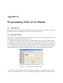
D Programming PALLAS in Matlab
D.1 Introduction . . . . . . . . . .
D.2 Matlab GUIDE . . . . . . . .
D.3 PALLAS GUI . . . . . . . . .
D.4 PALLAS program . . . . . . .
.
.
.
.
.
.
.
.
.
.
.
.
.
.
.
.
.
.
.
.
.
.
.
.
.
.
.
.
.
.
.
.
.
.
.
.
.
.
.
.
.
.
.
.
.
.
.
.
.
.
.
.
.
.
.
.
.
.
.
.
.
.
.
.
.
.
.
.
.
.
.
.
.
.
.
.
.
.
.
.
.
.
.
.
.
.
.
.
97
. 97
. 97
. 101
. 105
.
.
.
.
.
.
.
.
.
.
.
.
.
.
.
.
.
.
.
.
.
.
.
.
.
.
.
.
.
.
.
.
E STUNT Database
113
E.1 About the Database . . . . . . . . . . . . . . . . . . . . . . . . . . . . . . . . . . . . . 113
E.2 Design . . . . . . . . . . . . . . . . . . . . . . . . . . . . . . . . . . . . . . . . . . . . 113
E.3 Telemetry system: the weather forecast . . . . . . . . . . . . . . . . . . . . . . . . . . 114
F Detailed recommendations
115
F.1 Improving the Car Model . . . . . . . . . . . . . . . . . . . . . . . . . . . . . . . . . . 115
F.2 Sensors . . . . . . . . . . . . . . . . . . . . . . . . . . . . . . . . . . . . . . . . . . . 116
F.3 PALLAS programming . . . . . . . . . . . . . . . . . . . . . . . . . . . . . . . . . . . 118
G 2005 Panasonic World Solar Challenge
119
Bibliography
123
Chapter 1
Introduction & Problem Definition
1.1 Introduction
1.1.1
Solar Team University of Twente & the World Solar Challenge
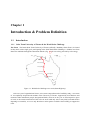
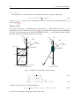
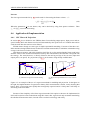
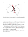
The Team The Dutch Solar Team University of Twente (officially ’Raedthuys Solar Team’) is formed
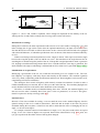
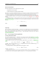
in May 2003 with a single goal: participating in the 2005 World Solar Challenge, a 3000 km race from
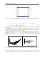
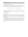
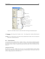
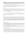
Darwin to Adelaide through the Australian outback (Fig. 1.1) for cars solely powered by solar energy.
Darwin
Katharine
Tennant Creek
Alice Springs
Coober Pedy
Port Augusta
Adelaide
Figure 1.1: World Solar Challenge race track (Stuart Highway).
After one year of organizational issues, active team composition and a feasibility study, a core team
of 14 completely inexperienced students of the University of Twente, supported by local business and
numerous other enthusiastic people, designed and built a solar car in one year. A most impressive piece
of work, as the actual construction of the solar car itself could only start in may 2005 (4 months before
departing to Australia), as it was only then that a main sponsor could be found willing to support the
team.
2
1. INTRODUCTION & PROBLEM DEFINITION
The WSC The World Solar Challenge is a bi-annual event, that is held for the eighth time in 2005.
Originally, it was a race for solar powered cars only (divided in ’production’ class for 2 or more persons
and larger solar arrays, and an ’open’ class, in which a car is allowed to carry only 1 person, but has
more restrictions in battery and solar array size). Nowadays, also a Greenfleet-class (using renewable
energy in general) and a Solar bicycle class (bicycling aided by solar power) are part of the World Solar
Challenge.
The Solar Team will participate in the ’open’ class race, which will take the team through the Australian Outback following the Stuart Highway.
The goal of the WSC is mainly to promote the use of renewable energy. More information can be
found on the WSC website www.wsc.org.au.
1.1.2
The SolUTra
A solar car is fundamentally built for efficiency and speed. Driver comfort, good looks and affordability
are secondary goals.
Most solar cars are of sleek design to minimize drag, with a large solar array on top to collect as
much solar power as possible. The SolUTra is not different. She has three wheels, as this results in less
roll friction, with 2 wheels in front and one in the rear, which is also the driving wheel. The electro motor
used is an ’in-wheel’ motor, which means that it is directly attached to the wheel. In this way, there is no
need for transmission anymore, increasing the efficiency of driving.
The design of the solar car consists of 3 main fields of interest: Mechanics, Electronics and Telemetry.
Mechanically, the car is designed for minimal drag and roll friction, while electronically, the car is
optimized for energy efficiency. Telemetry deals with measuring relevant quantities and transporting and
storing the measurement data.
Electronics The SolUTra contains a Worly Li-Polymer battery pack, that is charged via the AsGe-solar
array. 5 DriveTek Maximum Power Point Trackers ensure that the solar array delivers maximum power.
The battery supplies energy to an NGM brushless DC electro motor (combination of an NGM AC motor
and Tritium Gold DC/AC motorcontroller).
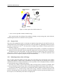
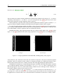
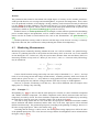
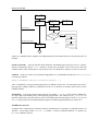
The battery also supplies power to the telemetry system, consisting of various sensors and a WLAN
system for communications with the chase car. See Fig. 1.2 for an overview of the basic solar car parts.
Mechanics Mechanical challenges in the SolUTra project consisted of designing a chassis of which
the drag is to be minimized, wheel spats that turn with the wheel, the suspension of the wheels that had
to fit in the chassis and a steering system for a car in which a steering wheel simply does not fit.
Telemetry Measurement data from the SolUTra is transported via a WLAN to the chase car. The chase
car contains some sensors as well, like a GPS and a weather station. All measurement data is stored in a
database for analysis or other uses
1.2 Problem definition
The main challenge of the STUT is to find a way to be the first team to arrive at the finish line, with
limited battery capacity and being compelled to using solar energy only.
To do this, the solar team has to:
1. strive to design and build a very fast and economic solar car;
PROBLEM DEFINITION
3
Figure 1.2: Basic parts of the SolUTra Solar Car
2. drive as fast as possible with the available energy.
This report describes the tackling of the problem of finding a racing strategy that, when followed,
would bring the SolUTra to Adelaide as fast as possible.
1.2.1
Project Goal
The goal of this graduation project is to develop an optimal racing strategy for the SolUTra solar car,
which minimizes the time needed for the SolUTra to reach the finish line. Although the SolUTra is able
to reach a car speed of over 100 km/h, she may not have enough energy available to keep top speed for the
total distance of the race.
Now, the problem can be regarded as a time-optimal control problem. An optimal car speed has to
be found, that controls the balance between input and output power such, that racing time is minimized.
The batteries act as an energy buffer. As long as the batteries do contain energy, the car speed can be
chosen freely. Otherwise, the car speed is constrained by the input power. It is therefore imperative, that
the batteries are never completely emptied (except at the finish line).
1.2.2
Balancing battery State-of-Charge
The car speed controls the balance between input power and output power and therefore the available
energy in the batteries, which, in turn, constrains the car speed. Thus, the car speed has to be chosen
such, that the SolUTra reaches the finish line as soon as possible, while satisfying the battery condition
of always having energy available in the battery.
The effect of a certain car speed on the battery State-of-Charge (SOC) can only be estimated, when
it can be predicted how much energy will be used for driving and how much energy will be collected.
It is therefore important to keep track of everything that will have influence on the amount of energy
used and collected. e.g. Cloud coverage results in less energy collected, as insolation decreases; the
presence of headwind will increase the power needed to maintain a certain car speed; speed limits restrict
the car speed, even if the battery SOC allows for high speeds.
4
1. INTRODUCTION & PROBLEM DEFINITION
There are a lot of factors that will influence the battery SOC. All these factors have to be measured
in some way in order to use them for power consumption predictions. Measurement and prediction
calculations can be automated in order to be able to provide information to the team as soon as possible,
as this information is to be used for planning. In this way, automation provides a way to calculate the
best way to use the available energy.
In other words, automation provides a way to design an optimal racing strategy, which brings the
solar car to the finish line as soon as possible.
1.2.3
Strategy Development Program
To automate the determination of an optimal racing strategy, a Strategy Development Program (SDP)
is to be designed. The task of the SDP is to develop a racing strategy, which is basically a car speed
setpoint to the car driver. The SDP can use all available data to perform its task, while being able to react
at changing situations.
The SDP has to calculate an optimal car speed guideline. The SDP must also be able to calculate a
new strategy, if the one adopted becomes useless. This happens when, for example, the car falls behind
schedule. As the chances of being thrown off-schedule by traffic lights, flat tyres and such, are so big
that it is virtually certain that this will happen, the SDP must be sufficiently robust to deal with such
stress situations. And it has to do this quickly, as it is advisable to follow the optimal strategy as much
as possible. This introduces a design requirement of being able to calculate the optimal strategy in mere
minutes.
On the other hand, a very accurate car model is desired for accurate simulation and optimization
and the SDP has to be provided with sufficient data and reliable predictions about the racing track in
order to be able to develop a feasible strategy. However, the original plan of using adaptive modeling for
improving the car model during tests had to be abandoned due to lack of time, so a static model has to
be used.
1.3 STUNT
The Telemetry system is managed by the STUNT network, the ’Solar Team Universal Network Technology’ network, which has been built by Vincent Groenhuis, the Solar Team Telemetrist. This network
collects all sensor readings and performs a fast scan of the data for alarming situations.
The network contains a MySQL database (the STUNT Database), which stores virtually everything
regarding the SolUTra project. Apart from the car sensor measurements, the STUNT Database holds an
electronic logbook, a list of static data (such as GPS positions, altitude, inclination, etc) regarding various
racing tracks, weather forecasts etc. The SDP is only allowed to make use of the STUNT Database. The
communication interface between the SDP and the STUNT Database is designed and built by Vincent
Groenhuis.
1.4 PALLAS
The name of the Strategy Development Program that is to be used by the Solar Team University of
Twente is ’PALLAS’, a name that refers to the goddess of wisdom (Pallas Athena) of the ancient Greeks.
She is often accompanied by a pet owl, which represents wisdom. Her attributes, however, often include
a lance, helmet and a shield, representing the intellectual aspect of warfare: strategy and tactics. She was
the goddess of the great leaders of ancient Greece and the patroness of the city of Athens.
REPORT OUTLINE
5
1.5 Report outline
The report starts with the design and the various aspects of the solar car model. Chapter 3 explains the
optimization of the racing strategy, while chapter 4 shows how PALLAS checks whether the solar car is
on schedule or not.
Chapter 5 treats the realization of PALLAS and chapter 6 shows how PALLAS is used during the
World Solar Challenge race.
One word of advice
A lot of the information on the SolUTra in this report has been retrieved by personal contact with the
experts and team members involved. A lot of this information has not yet been published and some will
never be. However, most information is crucial when considering all aspects involved in developing a
racing strategy. So, information from these sources is used in this report, despite the lack of references.
6
1. INTRODUCTION & PROBLEM DEFINITION
Chapter 2
Solar Car Model
2.1 Introduction
2.1.1
Model requirements
In order to calculate the impact of choosing a car speed on the battery SOC, a model has to be designed
of the solar car. This model has to approximate input power (Pin ) and output power (Pout ), while driving
an approximation of the racing track. The model must
• be able to estimate the amount of solar irradiance during the day, in order to calculate the input
power;
• be able to calculate the power delivered to the motor and the power dissipated in other electronic
systems;
• be able to handle various WSC regulations (media stops etc.);
• be simple enough, such that optimization does not take more than a few minutes;
• include a cost criterion that calculates the ’fitness’ of a strategy.
The relevant model outputs are the distance traveled and the battery SOC as functions of time, which
∗ (t).
basically describe a racing strategy, together with the optimal car speed vcar
2.1.2
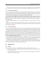
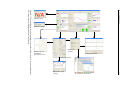
Model layout
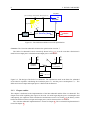
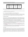
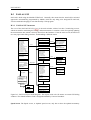
The general layout of the car model is shown in fig. 2.1.
The submodels of the model are:
Sun_Model This submodel calculates the perpendicular irradiance of the sun and the angle of the sun
above horizon as a function of time and location;
Road_Model The road submodel supplies the external circumstances, such as wind, slope, GPS position
etc. These circumstances depend on the location of the SolUTra in Australia;
Speed_Setpoint The speed setpoint submodel supplies the car speed setpoint vcar (t) to the Solar car
submodel. It takes account of media stops, overnight stops etc.;
Solarcar_Model The solar car submodel uses the data from the Road and solar models and the Speed
setpoint system to calculate the balance between input and output power and the battery SOC;
8
2. SOLAR CAR MODEL
Road_Model
(Sun Coverage, GPS position, Wind, slope etc.)
.txt
Road_Model
Sun_Model
Isol
γ
sun
Vcar
Speed_SP
v_car
road
SolarCar_Model
x
x
Criterion
SOC
SOC
Speed_SetPoint
Criterion
SolarCar_Model
Figure 2.1: The 20-Sim model that is used for optimization.
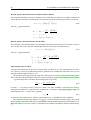
Criterion The Criterion submodel calculates the optimization criterion J.
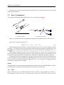
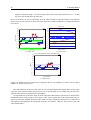
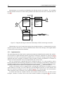
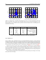
The Solar Car submodel is more extensively shown in Fig. 2.2. It can be seen that a distinction is
made between input power calculations and output power calculations.
γ
SC
CB
Isol
Vwind
Vcar
etc.
SC
CB
Isol
Vwind
etc.
sun
road
Insolation
equations
γ
sun
+
Pin
-
Pout
road
Power
Consumption
Battery
dQ(t)
= Pin - Pout
dt
Figure 2.2: The design of the Solar Car submodel. The calculations made in the Solar Car submodel
are devided in equations calculating the insolation power Pin and the power consumption Pout . The
difference between input and output power is buffered in the batteries.
2.1.3
Chapter outline
This chapter is dedicated to the implementation of the Sun submodel and the Solar car submodel: The
chapter starts with explaining the aspects of the solar car model regarding the power consumption and
subsequently, the equations which calculate the insolationare treated. In section 2.4, the battery, which
buffers the difference between input and output power, and its characteristics are treated.
The criterion submodel implementation is treated in chapter 3. The road model implementation is
treated in chapter 5.
POWER CONSUMPTION
9
The chapter on solar car model design finishes with an overview and characterization of the solar car
model and its parameters.
2.2 Power Consumption
The mechanical IPM and the bond graph of the solar car is shown in Fig. 2.3(a).
Fmotor
Vcar
Fdrag
Froll
I
Fslope
motor_current
α
MSe
Motor
TF
Wheel
1
Car
MSe
R
Roll
(a) Mechanical IPM
Gravity
Slope
MR
Drag
Wind
(b) Mechanical bond graph
Figure 2.3: The IPM and the corresponding bond graph of the mechanical aspect of the solar car.
The net force acting on the solar car is:
X
F = Fmotor − Fdrag − Froll − Fslope
(2.1)
When considering the fact that the car speed is assumed to vary little over time. Dynamical effects
regarding vcar are therefore relatively small, when compared to the large distance over which thePrace will
be simulated. So, simulation and optimization time can be greatly reduced by assuming that
F =0
in eq. 2.1.
This assumption neglects the energy lost to acceleration of the car. The car motor, however, may be
used as a generator when decelerating. In that way, some of the energy used for accelerating the car can
be regained (’regenerative braking’). Energy lost to inefficiency in regenerative braking is neglected.
An important result of this assumption is, that the car speed can be directly chosen, such that the solar
car inertia element in the bond graph of Fig. 2.3(b) becomes non-causal. This leaves only ’SolUTra’s
position (distance from Darwin) and battery SOC as car states. The output power can then be directly
calculated as a function of the car speed.
Outline
This Output Power section explains the implementation of the friction forces and the influence of slopes
on the SolUTra. It also briefly treats the electro motor used to drive the SolUTra.
2.2.1
Drag
Drag is the friction due to air flowing along the surface of the car. Drag depends on air density ρ,
the aerodynamic profile of the car CD and the square of the speed of the air flow relative to the car
10
2. SOLAR CAR MODEL
(~vcar − ~vwind ).
The Drag Force Fdrag acting on the car, caused by air flow and car speed, is defined by:
1
Fdrag = c(δ) · ~v 2 = ρCD (δ)Ad · ~v 2
2
(2.2)
in which CW (δ) = CD (δ)Ad varies with the angle of attack δ of the air flow and the top surface Ad of
the car (fig. 2.5(a)).
Effective air flow
The effective air velocity vef
~ f is determined by car speed vector ~vcar and inbound wind vector ~vwind . The
relation between these velocities is shown in fig. 2.4(a). This figure shows the direction (and magnitude)
of the car velocity and wind velocity in the local reference frame (Ψlocal ), which defines normal compass
directions. In order to calculate the effective air velocity:
north
Vcar
north
Ψlocal
∠φ
∠θ
Ψlocal
∠φ
wind
direction
Veff,x = Vw,x
Vcar
∠θ
wind
direction
east
east
Vw,y
Vw
∠δ
∠δ
Ψcar
Veff
Veff
Veff,y = Vw,y - Vcar
(a) Drag coefficient CW
Fdrag
(b) Approximation
Figure 2.4: Influence of wind and car speed on drag
vef f
=
p 2
(vy + vx2 )
(2.3)
vef f,x = vw sin(θ − φ)
vef f,y = vcar + vw cos(θ − φ)
2
⇒ vef
f
2
2
= vcar
+ 2vcar vw cos(θ − φ) + vw
(2.4)
And thus, for the drag force, the following applies:
1
2
2
Fdrag = ρCW (δ) · (vcar
+ 2vcar vw cos(θ − φ) + vw
)
2
in which CW (δ) depends on the angle of attack of the wind.
(2.5)
POWER CONSUMPTION
11
Drag parameter CW
Fig. 2.5(a) shows the dependency of CW of δ, measured using a scale model of the solar car in a wind
tunnel (Putten, 2005). CW is approximated by eq. 2.6 (Ad = 9 m2 ).
Cw (0, 1)
Drag coefficient Cw
0.1
0.08
0.06
Cw
(0, 0)
0.04
−δ
Cw
δ
Cw
0.02
0
−10
(a) Air speed components
−5
0
δ
5
10
(b) Drag force
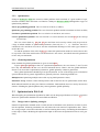
Figure 2.5: Cw as function of angle of attack)
CW (δ) = 9(−1.6 · 10−5 δ 2 + 8.9 · 10−3 )
(2.6)
For small values (less than app. 5°) of δ, CW can be considered constant:
CW (δ) = 0.08
(2.7)
The wind tunnel test with the scale model is not followed by a test with the SolUTra herself. As the
scale model is ideal (drag surface is very smooth), while the SolUTra itself has a lot of drag surface
irregularities, the measured CW value is considered to be only a rough and optimistic estimation of
SolUTra’s drag coefficient. The dependency of CW on δ does apply to the scale model only.
Therefore, it is decided to use a constant value of the drag coefficient.
Air density ρ
The most widely used method of determining air density is the application of the CIPM-81/91 formula
recommended by the ’Bureau International des Poids et Mesures’ (BIPM), which is a rather complicated
equation. In an article without author (BIPM, n.d.) the CIPM-81/91 formula is given (eq. 2.8):
ρ=
pMa h
Mv i
)
1 − xv (1 −
ZRT
Ma
(2.8)
with p the air pressure, T the temperature, xv the mole fraction of water vapour, Ma the molar mass of
dry air, Mv the molar mass of water, Z the compressibility factor and R the molar gas constant.
It is, however, simpler to start with the relation of eq. 2.9 and to use an approximation rather then use
the complex relation of eq. 2.8.
p
(2.9)
ρ=
R·T
in which R is the gas constant for dry air, which is 287,05 J/kg·K.
12
2. SOLAR CAR MODEL
Pressure, Temperature and Humidity To correct for air humidity, (Shelquist, 2004) uses
ρ=
p
R · Tv
(2.10)
in which Tv is a virtual temperature, which depends on air humidity. Tv is approximated by:
Tv =
T
1 − c1 Ep
(2.11)
c1 Tc
E = c0 · 10 c2 +Tc
(2.12)
in which E is the saturation vapor pressure, which may be multiplied with the air humidity percentage to
retrieve the actual vapor pressure. The virtual temperature will rise with increasing humidity (E), which
causes the air density to drop.
Humidity has only a slight influence on air density compared to air temperature and air pressure. It
will, however, increase with high temperatures and low air pressure. But for the purpose of simplicity,
the influence of humidity is neglected. This still leaves the air density depending on temperature and
pressure. Using 2nd-order Taylor series to linearize eq. 2.9:
ρtaylor =
1
p0
p0
∆T
+
∆p −
RT0 RT0
RT02
(2.13)
with p0 = 1 · 105 Pa and T0 = 298 K.
Furthermore, most weather types combine high temperatures with increased pressure, while low
pressure is often accompanied by bad weather and low temperatures. This means that the air density is
expected to vary only a little around ρ0 = 1.17kg/m3 .
Height
is:
According to (Tokay, 2005) (in which (Moran & Morgan, 1995) is cited) the air pressure at h
gh
p(h) = p(0) · e− RT
{mBar}
(2.14)
with g the gravitational constant, h the height in meters, R the gas constant and T the absolute temperature. As eq. 2.9 applies, the relation between air density ρ and the height is:
gh
ρ(h) = ρ(0) · e− RT
{kg/m3 }
(2.15)
However, (CSGnetwork, n.d.) uses eq. 2.16 for calculating the height h as a function of air pressure p
and sea level air pressure p0 :
p
h = 44308(1 − ( )0.190284 )
(2.16)
p0
This function can be linearized for p ∈ [800, 1050] mBar to:
h = 9(p0 − p) ⇒ p = p0 −
h
9
(2.17)
which, suggests a decrease of 90 mBar for each 1000 m. of altitude for p ∈ [800, 1050]. This can be used
as a rule of thumb.
POWER CONSUMPTION
2.2.2
13
Roll Friction
Roll friction is the friction of the tyres on the road and the bearing of the axes. This quantity depends on
the quality of the tyres, the quality of the road and the weight of the car. Although roll friction is defined
in various ways, Tamai uses ((Tamai, 1999), p5-6):
Froll = crr · w = (cr1 + cr2 · vcar ) · mcar · g
(2.18)
With mcar · g the normal force, which is assumed to be equal to gravity.
One may argue that driving on a sloped surface implies a decrease of the normal force, which results
in less roll friction. This effect, however, may be neglected; even in the case of an unlikely 10% slope
(10% ∼
= 5.7 deg), the decrease of the normal force is less then 0.5%.
cr1 depends on the type of the tire, road quality, the number of tyres etc. (static roll fiction), while
cr2 characterizes the speed dependent factor (dynamic roll friction). However, traditionally, the speed
dependent factor (cr2 ) is not included in the definition of roll friction, because the constant roll friction
is relatively big compared to the dynamic roll friction. In the case of this project, the static roll friction
factor cr1 is, however, small compared to the the dynamic roll friction. Therefore, dynamic roll friction
is included as well.
Characteristics are normally marginally provided by tire manufacturers. Tamai ((Tamai, 1999), p6)
however, provides parameter values of the best tire at that time (Michelin Radial tubeless, 1999):
cr1 = 0.0023
cr2 = n · 4, 1 · 10−5
(m/s)−1
(2.19)
with n the number of wheels. These parameter values are provided for smooth, regular, dry, open asphalt
roads.
This leaves questions about the magnitude of the roll friction for other surface types, such as gravel,
sand, sand on asphalt etc. To correct for these uncertainties, a system of roll friction classes is created:
the roll friction coefficients are multiplied with a factor that depends on the roll friction class of the road.
2.2.3
Gravity
The gravity force due to sloped terrain (fig. 2.3(a)) depends on the car weight. When the car ascends a
hill, gravity pulls the car backwards. The magnitude of this force is:
Fgrav = mcar · g · sin(α)
(2.20)
in which α is the angle of the slope.
2.2.4
Direct-Drive Electric motor & Motor Controller
The Solar Team University of Twente uses the Biel Solar Motor 2005 (BM-5) (Vezzini & Jeanneret,
2005) of DriveTek. The motor is especially designed for the WSC 2005. This BM-5 motor is a directdrive brushless DC motor that can be attached to the car wheel, such that no transmission occurs between
the motor and the wheel.
The typical optimal input power range for direct-Drive solar motors is 1 - 2 kW, as the output of the
solar panels that are used in the World Solar Challenge mostly is in that range as well.
The motor is supplied in combination with the Tritium Gold motor controller (Tritium Pty Ltd, 2003),
which can also be used in reverse mode, such that kinetic energy can be transformed into electric energy
when braking (regenerative braking).
14
2. SOLAR CAR MODEL
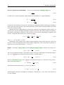
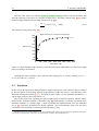
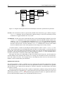
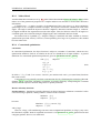
The Biel solar motor user manual (Vezzini & Jeanneret, 2005) provides some measurement data
about the efficiency of the motor as a function of input power. This data is shown in fig. 2.6. A simple
numerical approximation has been made and given in eq. 2.21.
ηm =
196.7
arctan(0.25(Pin + 100))
π
(2.21)
This function is also plotted in fig. 2.6.
Motor efficiency as a function of input power
98.4
98.2
98
97.8
Efficiency{%}
97.6
97.4
97.2
97
96.8
0
500
1000 1500 2000 2500 3000 3500 4000
Input Power {W}
Figure 2.6: Approximation of the efficiency of the Biel Solar Motor 2005 (BM-5) as a function of input
power according to expectations
Although the motor efficiency varies with the motor input power, it is fairly constant (ηmotor =
98.2%) for values of > 1000 W.
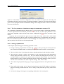
2.3 Insolation
In this section, the input power implementation is treated. Input power is the amount of power collected
by the solar panels. This quantity depends on the efficiency of the solar cells (ηp ), the efficiency of the
Maximum Powerpoint Trackers 1 ηmppt , the effective panel surface (A), the maximum insolation (Isol )
and the angle of the sun above the horizon (γ).
This section starts with explaining the general input power (insolation) equation, which is implemented in the ’Insolation equations’ submodel in Fig. 2.2. Subsequently, it treats the calculation of the
maximum insolation Isol and the angle γ, which is basically the implementation of the Sun submodel
in Fig. 2.1. After this, the MPPT’s are briefly explained. This section finishes with a test run of the
calculation of the insolation for each moment in time during 1 day.
1
Maximum Powerpoint Trackers (MPPT’s) are used to maximize solar panel output by tracking the ’Maximum Powerpoint’
in the panel’s VI-characteristic, which may vary depending on insolation, panel temperature etc.
INSOLATION
2.3.1
15
General Insolation
Insolation consists of 3 types of insolation of which ’Direct Beam’ and ’Diffuse’ insolation are the most
important.
Direct Beam Direct Beam Insolation is sunlight that arrives at the solar panels in a straight line from
the sun.
Diffuse Diffuse Insolation is indirect insolation due to the scattering of sunlight caused by dust, clouds,
haze, fog etc. Diffuse sunlight is unfocused light, which comes from everywhere.
Reflections Sunlight reflected by earth and surroundings (buildings etc.). As this type of insolation
is unlikely to be very large compared to Direct Beam and Diffuse Insolation (the solar array is
directed to the sky, so surrounding reflections are unlikely to reach the array), it will be neglected.
The input power equation is (Trottemant, 2004):
Pin = ηp · ηmppt · A · (IDirect + IDif f )
(2.22)
Although direct beam insolation is relatively easy to calculate, diffuse light insolation is not. The
following approximation for Pin is used by (Trottemant, 2004) (eq. 2.23):
Pin = ηp · ηmppt · A · SC · sin(γ) + (1 − SC) · CB · Isol (γ)
(2.23)
In which SC is the ’Sun Coverage’ percentage, which is the amount of irradiance that is not blocked by
clouds etc. CB is the ’Cloud Brightness’ percentage, which represents the ’haziness’ and the level of
cloud refraction. γ is the angle of the sun above the horizon, while Isol (γ) is the maximum insolation
due to atmospheric scattering and absorption, which depends on the observer’s position, the time of the
day and the time of the year.
The sun coverage and cloud brightness parameters will have to be predicted before optimization.
They can be measured for analysis afterward.
2.3.2
Maximum Insolation (Sun submodel)
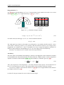
The maximum Insolation Isol (γ) depends on the angle of the sun above the horizon (altitude angle γ). If
γ is small, solar rays will have to travel a larger distance through the earth’s atmosphere, while attenuated
by scattering and absorption.
The effect of atmospheric attenuation can be calculated using the definition of ’Air Mass Index’,
which is a measure of the amount of air the sun rays have to travel through ((Liu, 2001)). The maximum
insolation is approximated by (Liu, 2001 (Liu, 2001)):
0.678
Isol (m) = 1353 · 0.687m
in which
m=
{W/m2 }
1
sin(γ)
(2.24)
(2.25)
The altitude angle γ depends on location (longitude & latitude), the earth’s declination, the time of year
etc. In the same paper, a calculation of the angle γ is provided:
sin(γ) = [sin(lat) sin(decl) + cos(lat) cos(decl) cos(H)]
(2.26)
16
2. SOLAR CAR MODEL
Solar Irradiance
Solar_Power {W/m2}
1000
Summer
800
25 Sept.
600
Winter
400
200
0
0
5
10
15
20
time {hr}
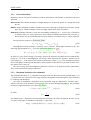
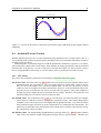
Figure 2.7: Solar Irradiance (Isol (γ) · sin(γ)) at mid-summer (December 21), mid-winter (July 21) and
at the 25th of September (start of the race)
with H the hour angle, lat the latitude and decl the declination of the earth.
360
[N − th − h0 ]
24
EOT
ψlocal − long
N = 12 +
+
60 15 284 + d
decl = 23.45 · sin 2π
365
H =
{deg}
(2.27)
{hr}
(2.28)
{deg}
(2.29)
with N the local noon time, EOT an ’Equation of Time’2 , long the longitude, ψlocal the local
meridian, th − h0 the time difference from solar noon time and, finally, d the day of the year (32 = 1st of
February).
The result (Isol (γ) sin(γ)) as a function of time is shown in fig. 2.7. Insolation is plotted for three
different days of year (at Alice Springs, AUS, app. 130◦ long., −20◦ lat.). The difference between winter
time and summer time is distinct.
2.3.3
MPPT’s
The Solar car is equipped with New Generation maximum powerpoint trackers (MPPT’s). These devices
track the so-called maximum power point, which is the point at which the power transferred to the load
(fig. 2.8(b)) is maximum. The MPPT device changes the input/output current ratio by varying the output
voltage until the maximum power point {Vmpp , Impp } has been found (fig. 2.8(a)).
The MPPT that is used by the solar team is the MPPT New Generation of the University of Applied
Sciences of the Biel School of Engineering (Biel School, 2003), which is a 200/800W DC/DC Maximum
Power Point Tracker with boost converter meaning that the output voltage is always higher then the input
voltage. 5 MPPT’s are used simultaneously in the solar car.
The MPPT functions optimally with an input power of between 200 and 800W at temperatures between 0 and 70 degrees Celsius. The optimal efficiency of the MPPT is 98.8% at an output voltage of
2
An approximation of the EOT is: EOT = 10.2 sin(4π d−80
)−7.74 sin(2π d−8
) ∼ 0.34(d−268)+8.2
373
355 =
(Satel-Light, n.d.)
d ∈ [268, 277]
INSOLATION
17
I
out
Iclosed
Impp
SolarCell
Vmpp Vopen
V
(a) Photo-voltaic cell characteristic
Load
out
(b) Single Solar cell with load
Figure 2.8: Single solar cell curve and connection circuit
130 V, an input voltage of 110 V and an input power of 300 W. The MPPT efficiency for a single MPPT
as a function input power is shown in fig. 2.9.
MPPT
100 100
16
90 90
14
80 80
12
70 70
10
approximation (%)
MPPT eff. (%)
error (%)
60 60
8
50 50
6
40 40
4
30 30
2
20 20
0
10 10
-2
0
0
0
100
200
300 400 500 600
MPPT Input Power
700
800
-4
Figure 2.9: MPPT efficiency as a function of input power and the approximation
The MPPT efficiency curve can be approximated by:
ηmppt = 100 arctan(0.225Pin ) − 0.003Pin + 0.8
However, the MPPT efficiency can be considered constant over a wide range (input > 100 W). It is
only when input becomes lower then 100 W, that MPPT efficiency significantly decreases.
2.3.4
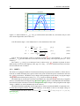
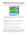
Input power testing
Fig. 2.10 shows the results of the implementation of eq. 2.23. The input power is calculated for the 25th
of September at the location of Darwin, NT, with a Sun Coverage SC of 100%, a panel efficiency ηp of
23%, an MPPT efficiency ηmppt of 98% and a solar array area A of 7 m2 (values provided by Electrical
Engineering Division of the Solar Team).
18
2. SOLAR CAR MODEL
Input power
Max. Insolation {W/m2}
Input Power {W}
Charge {kWh}
1400 1400
14
1200 1200
12
1000 1000
10
800 800
8
600 600
6
400 400
4
200 200
2
0
0
0
6
8
10
12
time {hr}
14
16
18
Figure 2.10: Input power simulation. This figure shows the Maximum Insolation Isol (t) , the resulting
input power Pin (t) and the total collected energy during one day of charging. The location is Darwin,
NT, and the Sun Coverage SC is 100%.
The figure shows that a maximum input power of slightly more than 1400 W and a total amount of
collected energy of ca. 11 kWh can be achieved on a cloudless day. The figure also shows discontinuities
at 8 a.m. and 5 p.m. These result from the regulation that cars are only allowed to drive between these
moments. Before 8 a.m. and after 5 p.m., the team is allowed to point the solar array directly at the sun
( or sin γ = 1).
However, clouds at the horizon, imperfect aiming of the array at the sun and decreasing MPPT
efficiency may cause lower input power. So the input power calculation is multiplied with parameter ηec
which models the effectiveness of these charging sessions before and after racing time.
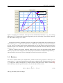
2.4 Batteries
The solar car model is built up of a simple battery, which stores the energy surplus, or makes up for an
energy deficit. Pin is the power gained from the solar panels, which is already already defined in eq. 2.23.
Pout is the power used for driving the car, which is the sum of all power lost to friction, resistors (e.g.
motor efficiency) and other power consumers (P0 ), like the radio and the sensors.
Q(t) = Q(t0 ) +
with Q(t) the battery State-of-Charge.
Z
t
t0
(Pin − Pout )dt
(2.30)
BATTERIES
2.4.1
19
Worley’s lithium polymer cells
The solar car batteries are Worley Lithium Polymer cells, produced by KOKAM. These batteries have a
very high energy density (0.180 kW h/ kg which makes them very attractive for usage in solar cars, where
mass is considered to be a critical parameter.
The Worley battery is a 3350 mAh battery cell. The battery pack of the solar car consists of enough
cells to hold at least 5 kWh of energy, with a maximum weight of 30 kg. in accordance with the regulations.
Also, the efficiency of this type of battery contributes to the attractiveness of lithium polymer batteries. When used properly, 99% of the energy stored in the battery can be recovered.
2.4.2
Battery SOC measurement
One of the hardest quantities to measure of the solar car is the battery State-of-Charge, which will have
to be measured indirectly, by keeping track of the battery current. The battery state-of-charge is the
time-integral of the battery current.
Using a current measurement to keep track of the battery SOC, however, will be inaccurate as each
offset on the current measurement is accumulated, causing drift in the SOC measurement.
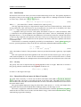
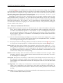
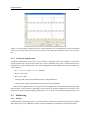
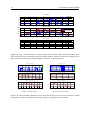
The output voltage of the battery is not a good measurement of the battery SOC either, as is shown
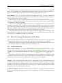
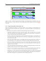
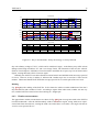
by the discharge current curves of the Worley lithium polymer cell (Worley, 2004) in fig. 2.11. This
figure shows the battery output voltage at various constant discharge current rates. As the solar car
typically does not use constant battery currents, these output voltage curves cannot be used for battery
SOC measurements.
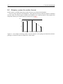
Figure 2.11: Single cell battery discharge curves at various discharge currents for the Worley 3350 mAh
lithium polymer cell. It can be seen that the energy recovery rate of the battery decreases at higher
currents.
20
2. SOLAR CAR MODEL
A solution to this problem is to use a highly accurate current sensor for battery current measurements
in combination with a periodic calibration of the battery SOC measurement. The measurement can be
calibrated by using an ’equilibrium curve’.
Battery states
According to (Valer Pop, 2005) a battery or accu can be in one of the next 4 states:
Charge Battery SOC increases, caused by an input current;
Discharge Battery SOC decreases, caused by an output current;
Transit Battery current has decreased below 0.05 CmA, either charging or discharging;
Equilibrium The battery enters equilibrium state after being in Transit state for at least 2 hours, depending on the type of battery.
When in equilibrium state, the battery SOC can be estimated with fair accuracy by measuring the
output voltage and correcting for battery temperature (the accu pack used in Australia contains temperature sensors). In that case, the plot of fig. 2.11 is again used, with the discharge current curve of <0.05
CmA, which can be gained by extrapolating or, better, measurement. In that case, a discharge curve of
at most 0.05 CmA should be used (taking 20 hours to fully discharge).
Example
Suppose a electric device that requires a constant supply current of, conveniently, 0.5 CmA. The battery
output voltage will behave like the 0.5 CmA curve in fig. 2.11. After 4 hours of continuous discharge
(2000 mAh), the battery output voltage will be approximately 3.63 V.
If the device is shut down, the battery will enter transit state. if the device is not powered up in the
next 2 or 3 hours, the battery will slowly enter equilibrium state: the battery output voltage will rise
slowly until the equilibrium curve is reached, where it will settle.
Extrapolating from the curves, that have already been measured, the equilibrium curve will be approximately 3.9 V.
Australia
When using these batteries during the solar challenge race, the battery SOC are estimated by using
voltage and current measurements. Calibrating the SOC measurement can be done each day after having
had a whole night to enter the equilibrium state and before the racing starts at 8 ’o clock in the morning.
When calibrated, the initial battery State-of-Charge is known and a new strategy can be developed.
However, temperature does have its effect on the equilibrium curve, so the initial state-of-charge measured may not be very accurate ((Worley, 2004), sheet 9).
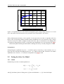
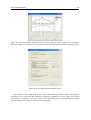
2.4.3
The SolUTra battery
Measurement
The battery pack of the SolUTra consists of 25 battery packs connected in series and it is fitted with
a LEM LAS 50-TP/SP1 current transducer, which boasts an inaccuracy of less than 1% (not including
electric and magnetic offsets, and linearity error). Each battery pack consists of 18 previously described
TESTING THE SOLAR CAR MODEL
21
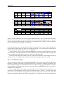
105
Battery output voltage (V)
100
95
90
85
80
75
0
1
2
3
4
5
6
Battery charge (kWh)
Equilibrium Curve (3A Charge)
Extrapolation of linear area
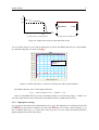
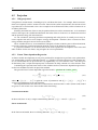
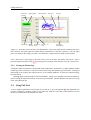
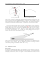
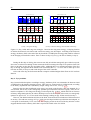
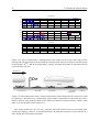
Figure 2.12: Equilibrium curve of the SolUTra racing battery pack, using a charge current of 3 A ∼
= 0.04
CmA. Only half of the measurements were performed. The extrapolation is also shown.
Worley lithium-polymer battery cells in parallel. In the days before the 25th of september 2005, the
battery cells were properly balanced and the battery equilibrium curve was measured, using a charge
current of exactly 3A, which is slightly less than 0.05 CmA. Due to circumstances, the charging time
was limited to approximately 10 hours, so only half of the equilibrium curve was measured (Fig. 2.12).
When leaving Darwin during the World Solar Challenge, the battery was fully charged to 6.2 kWh.
Extrapolation
Extrapolating the equilibrium curve for > 2.5 kWh is prone to inaccuracy, as the sensitivity kW h/ V is
large, due to the fact that the equilibrium curve for > 0.5 kWh is relatively flat. In absence of a reliable
equilibrium curve for SOC > 2.5 kWh, the extrapolation of fig. 2.12 is used.
2.5 Testing the Solar Car Model
2.5.1
Model
Summarizing, the solar car model equations are
Q(t) = Q0 +
x(t) = x0 +
Z
t
t0
Z t
(Pin − Pout )dt
vcar (t)dt
t0
with Q(t) the battery State-of-Charge and x(t) the traveled distance. vcar (t) is the model input.
22
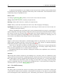
2. SOLAR CAR MODEL
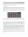
Quantity
Car parameters.
Aerodynamic profile (est.)
Vel.-indep. roll fric. coef.
Vel.-dep. roll fric. coef.
Car mass
Solar Panel eff.
MPPT eff.
Solar Panel Surface
Default Motor eff.
Other parameters.
Regen. brake eff.
Charge effectiveness
Default Air density
Number of wheels
Const. Power factor
Local meridian
abbr.
CW (δ)
cr1
cr2
mc
ηp
ηmppt
A
ηm
ηrb
ηec
ρ
n
P0
ψlocal
value
unit
source
0.08
0.0023
4.1 · 10−5
280
23
98
7.092
98
(m/s)−1
kg
%
%
m2
%
Estim. by Aero. div.
(Tamai, 1999)
(Tamai, 1999)
Estim. by Mech. div.
Estim. by Elect. div.
section 2.3.3
Estim. by Elect. div.
section 2.2.4
60
70
1.17
3
∼23
127.5
%
%
kg/ m3
W
°
Estim. by Elect. div.
section 2.3.4
section 2.2.1
Observation
Estim. by Elect. div.
+9.5 Time zone
Table 2.1: (constant) Car parameters (of which some are estimations by various divisions of the Solar
Team). The primary car parameters are the most important characteristics of SolUTra.
The equations for input and output power are
Pin = ηp · ηmppt · A · SC · sin(γ) + (1 − SC) · CB · Isol (γ)
1 1
2
Pout = P0 +
ρCW (δ) · vef
+
m
g
·
(sin(α)
+
n
·
c
)
·
v
+
m
g
·
c
· vcar
c
r2
car
c
r1
f
ηm 2
In this case, the motor efficiency is assumed to be constant. However, the motor efficiency varies
with the motor speed and torque.
2.5.2
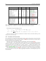
Parameters & Characteristics
The car parameters are summarized and quantified in table 2.1.Some of the parameter values in this table
have been obtained from contact with team members of the Solar Team University of Twente and are
therefore indications of the real parameter values.
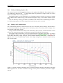
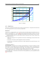
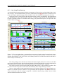
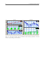
With these values the following output power characteristic can be derived (fig. 2.13).
From this figure, it can be derived that with this parameters, the roll friction exceeds air friction
when the car speed is lower than 50 km/h. Above 50 km/h, air friction is the dominant friction factor.
A characteristical value is the output power at 100 km/h, which is ≃ 1500 W for the SolUTra in this
configuration. This is a relatively low value, when compared to the 1650 W of the NUNA III, this year’s
champion (van Velzen, 2005), so the car is either very good, or the car parameters may be very optimistic.
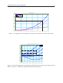
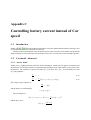
The output power is plotted in fig. 2.14 for various slopes. It can be seen that output power doubles
between 80 and 100 km/h in case of a 1° slope, suggesting the importance of measuring the slope of the
road beforehand.
TESTING THE SOLAR CAR MODEL
23
Output Power
2500
Pout {W}
Pdrag {W}
Proll {W}
2000
1500
1000
500
0
0
20
40
60
Car Speed {km/h}
80
100
120
Figure 2.13: Output power and components as a function of car speed on a flat road with no wind
Output power at various slopes (deg)
Pout {W}
5000
4000
2.5°
1°
3000
0°
2000
-1°
1000
0
-1000
-2.5°
-2000
-3000
0
20
40
60
80
x {km/h}
100
120
140
Figure 2.14: The total output power (including drag and roll friction) at various slopes. Between 80 and
100 km/h, a slope of 1◦ doubles the output power needed to maintain speed.
24
2. SOLAR CAR MODEL
Chapter 3
Strategy Optimization
A man who does not plan long ahead will find trouble right at his door.
– Confucius
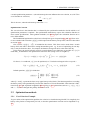
3.1 Introduction & Optimization Problem
In this chapter, the optimization problem (OP) and the ways to solve this problem are treated. The
chapter starts with a description of the optimization goals. These goals are translated into a Cost Criterion
function. Then, some methods for optimization are treated. In the last section, a possible implementation
of optimization in PALLAS is suggested.
The emphasis of developing a strategy is on finding an optimal solution to the OP in a fast and reliable
way.
For simplicity, car speed is now represented by v(t) instead of vcar (t).
3.1.1
Optimization goals
Speed
The OP that is to be solved by the SDP is basically a time-optimal control problem and a minimization
(eq. 3.1) of the time te needed to travel a certain distance xtotal , which is the total distance from start to
finish.
Z
te
min J =
dt = te
(3.1)
0
The solution to this OP is the highest average car speed achievable. During the race, input and output
power are to be carefully balanced, as the only power available for driving is gained from the solar panels
and no other power source may be used.
Efficiency
The car’s efficiency is measured by the energy used to move the car over a fixed distant xtotal in a fixed
amount of time te . This can be translated to displacing the car with a limited amount of energy in a
certain amount of time. Maximizing efficient use of available energy means therefore minimizing eq.
3.2.
Z
te
min J =
0
−v(x, t)dt = −xte
(3.2)
26
3. STRATEGY OPTIMIZATION
Solution to the Optimization problem
The Solar Car model, which is designed in chapter 2, is used for calculating the results of various strategies. The input of this model is SolUTra’s car speed v(t). The eventual solution to the OP will therefore
be an optimal car speed function v ∗ (t).
3.1.2
Criterion & optimization constraints
The criterion is to be designed while keeping a close eye on the requirements of the method that is used
to optimize the racing strategy.
Constraints
The solar car has a strict constraint on battery usage: the battery SOC is not allowed to be less then 0
kWh, nor is it allowed to exceed the maximum charge of approximately 6.2 kWh (section 2.4.3). It is
recommended to stay away from these limitations, as empty batteries result in the unfavorable situation
that the driver is restricted to a low maximum car speed (depending directly on input power) and fully
charged batteries result in a situation in which the energy surplus cannot be stored.
Uncertainty in weather expectations, road measurements, or parameter estimations may cause situations as described above. These situations can be avoided by using ’safety regions’: the normal ’operational range’ of the battery is set to be between ca. 10% and ca. 90% of full battery charge. In the event of
getting more or less solar energy then expected, these safety zones guard the occurrence of unfavorable
situations. Using the safety zones should be punished when calculating an optimal racing strategy
These safety zones do not apply in the vicinity of either start and finish. At the starting line, the
batteries are allowed to be completely charged. At the finish line, however, efficient use of energy
demands the batteries to be almost exhausted, as energy left-overs could have been used for more speed.
Apart from battery SOC constraints, there are some other aspects that may constrain optimization:
Speed limits Speed limits apply to parts of the road between Darwin and Adelaide. These speed limits
vary from 50, 60 or 80 km/h in towns and cities, while a maximum speed of 110 km/h applies to the
whole of the state of Southern Australia. Serious cases of speeding may lead to disqualification;
Battery discharge current The battery SOC depends on the discharge current: larger discharge currents
wear the battery. So, large discharge currents should be avoided;
Motor efficiency Each motor has a region in which efficiency is optimal. Using that region as much as
possible is an energy efficient way of driving. Especially when using a direct-drive motor, as no
transmission is used to keep the motor functioning optimally efficient;
Choosing camping sites Choosing a camping site at which the car can still collect solar energy at the
end of the day will result in better initial conditions for the day after. This may be implemented by
imposing penalties on certain values of x(te ), but this will also generate local minima, complicating global optimization.
Optimization Parameters: Stages & time steps
As already stated, the result of the optimization should be an optimal car speed function v ∗ (x, t). To
calculate v ∗ (x, t), Pontryagin’s Minimum Principle may be used (see appendix A): analytically solving
the OP by writing the dynamic equation as a first order differential equation with a number of initial and
end values. The OP is rewritten to a Hamiltonian (Zwart & Polderman, 2001). However, this method
INTRODUCTION & OPTIMIZATION PROBLEM
27
is complex, and cannot be solved by symbolical computer programs like MAPLE (Schutyser, 2005).
Instead, Schutyser (Schutyser, 2005) suggests solving the OP numerically. Pudney (Pudney, 2000),
however, has solved the OP analytically (which is briefly explained in appendix C), but he had to rely on
shot methods to find the optimal starting conditions and concluded that his analytical solution to the OP
was an improvement of mere minutes of the strategy of maintaining a constant speed for the complete
distance of the race.
Trottemant (Trottemant, 2004) suggests the use of stages for numerical optimization: the complete
distance is divided in a certain number of stages. For each stage, a constant optimal average speed
v ∗ (x) is calculated. In this way, a set of optimization parameters is created, which consists of as many
parameters as there are stages. The benefits of using stages are:
• Improved calculation speed:
– v(x, t) is simplified to a vector of constants (~v ).
– Optimization over a smaller distance or time interval takes less time, as the set of optimization
parameters is smaller.
• The number of stages, and the distribution of stages over the racing track may be changed according to the most recent situation (changing weather etc.);
• When x(te ) is fixed (end value problem), the number of optimization parameters is constant, thus
avoiding situations in which parameter values do not have effect on the cost criterion at all, resulting in an infinite set of local minima.
Schutyser (Schutyser, 2005) suggests the use of time steps: vcar (t) is discretized to v(k) with a
certain time step tk . For each time step, an optimal value of v(k) is calculated. The set of optimization
parameters consists of as many elements as there are time steps. The benefits of using time steps are:
• The size of the time steps can be chosen beforehand. The size can even be variable during the race
(like variable sized stages);
• Using time steps resembles discretization of a continuous input signal, rather then using stages;
• When te is fixed, the number of optimization parameters is constant, thus avoiding situations in
which parameter values do not have effect on the cost criterion at all, resulting in an infinite set of
local minima.
However, media-stops (30-minute stops at certain locations) during the trip may complicate the use of
time steps as optimization parameters.
R
Time and distance are related via x(t) = v(t)dt. However, when speed is considered to be constant
during one stage or time-step, the interdependence can be simplified to:
xk = vk tk
(3.3)
in which vk designates the k-th car speed element in the optimization parameter set and tk is the k-th
time step. xk is the distance traveled during the k-th time step or stage.
When considering time steps and stages, stages are fitted for use when optimizing car speed for a
fixed distance (being as fast as possible), while time steps can be used when car speed is to be optimized
over limited time te (being as fast as possible, as well as being as efficient as possible). After all, an
unlimited amount of solutions may exist if a variable x(te ) resp. te is used. An example of this is when
28
3. STRATEGY OPTIMIZATION
a certain optimization parameter vi (the ith timestep) does not influence the cost criterion, or (with V the
set of feasible car velocities).
dJ
= 0 ∀ vi ∈ V
dv(i)
This is the case, when the ith timestep starts after t = te .
Optimization Criterion
The cost criterion is the function that is evaluated by the optimization method to decide which set of
optimization parameters is optimal. The optimization method may require the evaluation function to
meet certain specifications. Most gradient methods (see B.2.2) require the evaluation function to be
twice differentiable.
The fundamental optimization criteria have already been given in equations 3.1 and 3.2. These criteria are extended with a function g(Q(t)), which represents the battery safety limits, which are described
in section 3.1.2.
Also a factor w4 (Q(te ) − Q2des is included in the criteria. This factor can be used when a certain
battery SOC end value is desired for setting intermediate goals. e.g. In case of optimizing for one day
only. It may be desired to have, for example, the batteries charged for 60% at the end of the day.
Using stages, the goal is basically to travel a certain distance in as little time as possible. So, x(te ) is
fixed and te is minimized. The optimization criterion is then (using vector of weights w):
~
2
J(vcar ) = w4 (Q(te ) − Qdes (te ) ) +
Z
0
te
(w1 + w3 · g(Q(t)))dt
(3.4)
If a fixed te is considered, x(te ) is to be optimized, so J2 includes an integral of the car speed v.
2
J(v) = w4 (Q(te ) − Qdes (te ) ) +
Z
0
te
(−w2 · v + w3 · g(Q(t)))dt
(3.5)
In both equations, g(Q(t)) is defined as:

 (Q(t) − Q− )2 Q(t) < Q−
(Q(t) − Q+ )2 Q(t) > Q+
g(Q(t)) =

0
otherwise
(3.6)
where Q− and Q+ represent the lower resp. upper battery safety limits. The function penalizes exceeding
the battery safety limit quadratically, because this function is twice differentiable. This function is illustrated in fig. 3.1 and explained in appendix B.2.4. Using eq. 3.6, constraints (such as 0 ≤ x(t) ≤ x(te )
and vi > 0) can be changed into penalty functions as well.
3.2 Optimization methods
3.2.1
Cost Criterion: Example
To get a notion of the optimization problem, the criterion is visualized using MAPLE. For simplicity, the
battery safety limits are temporarily left out, so that the optimization criterion can be simplified to eq.
3.7.
OPTIMIZATION METHODS
29
10
9
8
g(Q)
7
6
5
4
3
2
1
0
0
1
2
3
4
5
SOC {kWh}
Figure 3.1: The safety regions of the battery. Including this function will prevent using those regions.



J = w1
Pn
xi
i=1 vi
+ w2 ·
Pn
Pin ≥ 0; Pout > 0; xi , vi >
xi
i=1 vi [Pin (xi , t)
P
0; ni=1 xi = C
− Pout (xi , vi )] − Qdes
2
(3.7)
in which cost criterion J1 depends solely on the end values of the car states (battery safety region is
not included).
A graphical representation of the cost criterion may be produced by setting up an experiment, consisting of a 100 km race. During this race, the input power is assumed to be constant, as well as disturbances,
like wind, which is assumed to be constant during a single stage.
The race consists of 2 stages of 50 km. each. A constant car speed is chosen for each stage. In fig.
3.2(a) the cost criterion for 10 < v1 , v2 W
< 100 m/s is plotted, showing a single minimum. Obviously, the
cost criterion is not defined for v1 ≤ 0 v2 ≤ 0, as these cases prevent the car from reaching the finish
line.
Optimization Criterion
2nd order Derivative test
250
0.02
200
100
v2
0.01
150
80
60
40
20
0
100
20
40
100
50
80
–0.01
60
40
20
0
v1
60
80
100
v2
–0.02
20
40
v1
60
80
100
(a) Cost Criterion
(b) 2nd Derivative test
Figure 3.2: The end values of cost criterion J for 2 stages resp. 2 timesteps optimization with MAPLE.
However, the plot also shows that near the axes (v1,2 → 0), the plot tends to decrease. This effect
is shown in fig. 3.2(b), which shows the value of the determinant of the Hessian of J. This is the ’2nd
30
3. STRATEGY OPTIMIZATION
derivative test’ (Weisstein, 1999b).
D=
∂2J
∂v12
∂2J
∂v2 ∂v1
∂2J
∂v1 ∂v2
∂2J
∂v22
(3.8)
This test shows the region in which gradient-based optimization methods will converge (D > 0), and in
which they will diverge (D < 0). The D = 0 curve is also plotted in fig. 3.2(b). This curve moves and
scales with variations in racing conditions (slopes, wind etc).
When optimizing, especially when using a gradient optimization method, regions in which D < 0
must be avoided, as gradient methods will diverge from the optimal solution in these regions.
To avoid diverging gradient methods, the battery safety region of eq. 3.6 is used to keep the battery
state of charge within acceptable and safe limits like a penalty function. This function is continuous and
twice differentiable, which is required in order to calculate the Hessian.
Including the battery safety regions generates the cost criterion surface plane of fig. 3.3(a). In this
figure, J1 (eq. 3.4) is plotted for the same racing experiment of fig. 3.2(a). Even exceeding the battery
40
40
35
35
30
30
90
90
80
80
70
70
v2 (m/s)
50
60
v2 (m/s)
60
25
50
25
40
30
40
20
20
15
15
30
20
10
20
10
0
0
10
10
15
20
25
v1 (m/s)
(a) Stages
30
35
40
10
10
15
20
25
v1 (m/s)
30
35
40
(b) Time steps
Figure 3.3: 2 stages optimization with MATLAB, including battery safety regions.
safety limits for just a little time causes the cost criterion to skyrocket. The area in which the optimal
parameter values are located is clearly visible as a long narrow tinted area. While the derivative of the
function large outside of this area, it tends to decrease fast when approaching the optimal solution.
Although all circumstances are equal during both stages, the MATLAB results show that the ’optimal
area’ around the optimal solution is not symmetric: J(v1 , v2 ) 6= J(v2 , v1 ). This is caused by the fact
that the input power is not zero, which causes battery overflow in case of driving too slow. Therefore, it
does matter whether one drives slow at first or at last.
Also shown is a plot of J2 (eq. 3.5) in which te = 2 h. This two-hour race is divided in two (n = 2)
time steps of 1 h. each. Also in this case, car velocities may not be less then 0, as the car model can only
be applied for car velocities above zero. The fact that this cost function is non-convex is clearly visible.
OPTIMIZATION IN PALLAS
3.2.2
31
Optimization
Schutyser (Schutyser, 2005) has treated a similar problem which consisted of a great number of optimization variables and a non-linear cost function. Schutyser (Schutyser, 2005) distinguishes 4 types of
optimization problems:
Linear programming problem The cost criterion is linear (or affine);
Quadratic programming problem The cost criterion is quadratic and the constraints are linear or affine;
Non-linear optimization problem The cost criterion is non-linear, non-convex;
Convex optimization problem The cost criterion is a convex function (see section B.1 for the concept
of Convexity).
The cost criteria (both eq. 3.4 and 3.5) are non-linear and convexity cannot easily be proved for
a large or infinite number of optimization parameters (Convexity for n → ∞). Therefore, the OP is
considered to be non-linear non-convex and the calculational advantages of the other types cannot be
used in this case.
To find the optimum of the OP in fig.3.2.1, a numerical optimization method is needed, that is able
to cope with a non linear model and a cost function that is not convex, and which cannot be guaranteed
to have only one minimum.
3.2.3
Global Optimization
Some methods for global optimization are given in sectionB.3.
Figures 3.3(a) and 3.3(b) show that, for 2 optimization parameters, the cost criteria (J1 and J2 ) each
have only one minimum. In that case, the local minimum that is found is also the global minimum.
However, for more then 2 optimization parameters, global optimality cannot be guaranteed.
Thus, global optimization should be given special attention. As one of the design goals is calculation
speed, methods such as genetic algorithms are generally ruled out. Promising methods are:
Multiple start Optimizing multiple times with varying initial parameter values;
Parameter sweep Evaluate various initial positions and use the best one for optimization (scatter shot).
Both methods benefit from using less function evaluations. Both methods, however, merely increase the
chances of finding the global optimum; they cannot guarantee global optimality.
3.3 Optimization in PALLAS
When designing an optimization algorithm for PALLAS, the design specifications of section 1.2 must be
observed: optimization should be fast and reliable and flexible.
3.3.1
Design choice: Splitting strategies
Numerical optimization methods need a certain amount of simulation runs (iterations) in order to calculate the optimum. Reducing simulation time will reduce the total amount of optimization time. Therefore, using a simple car model is advisable, as well as reducing the accuracy of modeling the disturbances
(wind, slopes, clouds). Reducing the optimization input set decreases the optimization time as well, generally.
32
3. STRATEGY OPTIMIZATION
To increase the strategy development speed, 3 different strategies are used. Developing a strategy for
the total remaining distance to Adelaide generally takes a lot of time, compared to developing a strategy
that lasts to the end of the day. Primary and secondary goals can be set, the primary being the total race
time from Darwin to Adelaide and the latter being at a certain location at the end of the day.
To put it simply: instead of continuously optimizing for the total distance of the race, a strategy is
developed for only a part of the race.
Start to Finish: Fixed distance (Long Term Strategy)
Considering the complete distance from start to finish, this distance has to be covered as soon as possible.
The total racing time te has to be minimized, while the battery SOC (Q(t)) is constrained (Battery SOC
may not exceed battery limits and should have a certain value at t = te ).
For Start-to-Finish optimization, Q(te ) should be 0, as all energy that is left in the batteries when
finishing could have been used for more speed. However, Q(te ) is physically limited and cannot be less
then empty.
The following applies
h
2
min w4 · (Q(te ) − Qdes ) +
v
h
Z
2
te
t0
i
[w1 + w3 · g(Q(t))]dt =
min w4 · (Q(te ) − Qdes ) + w1 · (te − t0 ) +
v
Z
0
te
[w3 · g(Q(t))]dt
(3.9)
i
in which λ is a weighing factor and te is the point in time the finish line is reached.
During the race, Start-to-finish planning can still be performed. However, the current position of the
solar car can be used as a starting point for the optimization, instead of the start of the race. Therefore,
’long term strategy planning’ may be a better definition of Start-to-Finish planning.
Simulating and optimizing could take a long time, when simulating for distances of thousands of
kilometers spanning multiple days.
Day-to-day racing (Mid Term Strategy)
Day-to-day racing means the situation of maximizing or chosing a certain desired distance and battery
SOC over a constant time interval [0, te ], while being constrained by battery SOC and speed limits. This
is exactly the case when optimizing for one day, when it is desired to reach a certain camp site at the end
of the day with as much energy in the battery as possible.
Z
h
2
min w4 · (Q(te ) − Qdes ) +
te
i
[−w2 · vcar + w3 · g(Q(t))]dt =
v
0
Z te
h
i
2
[w3 · g(Q(t))]dt
min w4 · (Q(te ) − Qdes ) − w2 · (x(te ) − x(t0 )) +
v
(3.10)
t0
In this case, the end-of-day value of the battery SOC (Q(te )) is the preferred initial battery SOC (Qdes )
for the next day of racing, which depends on the long term strategy, that is designed using long term
planning.
This day-to-day racing would be the ’normal’ strategy development routine during racing, as it is
assumed to take less time to develop a strategy.
OPTIMIZATION IN PALLAS
33
Short term planning (Short Term Strategy)
Short term planning basically is reacting to unplanned events. When something happens that endangers
the strategy planning, the SDP must be able to respond quickly. In that case, an optimization is to be
executed over limited distance xld , during which the battery SOC is to be closely guarded.
Z te
i
h
2
min w4 · (Q(te ) − Qdes ) +
[w1 + w3 · g(Q(t))]dt =
(3.11)
v
0
Z te
h
i
2
min w4 · (Q(te ) − Qdes ) + w1 · (te − t0 ) +
[w3 · g(Q(t))]dt
v
t0
The car should reach distance xld as fast as possible, constrained by the battery SOC, which should have
a certain value when xld is reached.
This optimization should be performed as quickly as possible, as the results are to be used immediately after optimizing.
Combining strategies
The 3 strategies that have been described in the previous sections may be used simultaneously. Startto-Finish planning may provide a planning outline for the complete track. Optimizing for the complete
racing distance may, however, take a lot of time, compared to day-to-day racing, especially for the first
days of racing.
Day-to-day planning takes the strategy outline given by long term strategy planning as a starting
point for optimization.
Optimizing over a short distance (Short term planning) takes less time than long term optimization
and day-to-day optimization. Therefore, it is a good option to use in case of unexpected events that cause
the car to diverge from the racing strategy. In that case, a new strategy is needed on short notice.
After developing and adopting a strategy for a short distance in short time (a couple of seconds), a
more accurate, although time-consuming (a couple of minutes), optimization for the total race can be
performed.
34
3. STRATEGY OPTIMIZATION
Chapter 4
Monitoring
However beautiful the strategy, you should occasionally look at the results.
– Sir Winston Churchill
4.1 Introduction
To guard the validity of the optimal strategy or planning, the real car states have to be compared to the
strategy. When ’monitoring’, the real car states and the strategy are plotted as a function of time in such a
way that the differences can easily be identified. An example of this is a driver who fails to keep optimal
speed and who drives constantly too slow. In that case, the solar car will fall behind schedule.
To counter the drift between reality and planning, one may shake up the driver upon identification of
the flaw between planned and real car speed, develop a new strategy or install a cruise control, the last
option being a structural, but presently, impossible solution.
In short, the course of events is as follows:
1. Check differences between strategy and reality for errors;
2. Identify the cause of the error;
3. Remove the cause of the error (e.g. a slacking driver), correct it (e.g. model errors) or compensate
for it;
4. Develop a new strategy in case the differences between planning and reality have grown to big.
This chapter starts with an overview of possible causes of future differences between strategy and
reality and the important variables that should be monitored. Then, some ways of monitoring the results
of the strategy are presented.
This chapter also treats some views at forecasting the future. When forecasting the future, drift
between the strategy and reality can be detected, before it actually occurs, thus increasing the response
time.
4.2 Model Accuracy
Differences between strategy and reality can be the result of either internal causes or external causes.
Internal causes consist of car model flaws. Fig. 4.1(a) shows that there are actually 2 models involved:
the Road model, which models aspects as wind speed and heading, clouds, slopes etc., while the Car
36
4. MONITORING
model consists of the equations mentioned in chapter 2. Both models are simplifications of the real
world and, thus, are subject to errors.
Road model
Car model
Road model
Car model
error
True Road
Solar Car
(a) Strategy monitoring
error
True Road
Solar Car
(b) Simulating for model adaptation
Figure 4.1: 2 models showing the difference between monitoring for strategy and simulating for model
adaptation.
External causes consist of flaws in the road model: weather predictions turn out to be incorrect, flat
tyres may happen, other road users may force the solar car to drive slower then planned.
Car model flaws may be decreased by measuring the inputs and outputs of the model (model validation as shown in fig. 4.1(b)) and in a similar way, the road model may be validated by measuring and
deriving all relevant parameters.
4.2.1
Car model
The Car model of fig 4.1 consists of calculating the input power, the output power and the charge of the
batteries. It also contains solar calculations (maximum irradiance and elevation angle). Although these
equations have already been treated in section 2, the possible inaccuracies are summed up here:
Drag Although tests have been carried out in a wind tunnel, these test were carried out using a downscaled model of the solar car and no tests will be carried out with the real solar car, reasons being
of a financial nature. If there happen to be any construction or scaling errors, they will not be
accounted for;
Roll Friction The parameters mentioned in section 2.2.2 are for the Michelin tyre, while the Solar Team
uses another type of tyre (Vredestein), of which the roll friction parameters have not yet been
determined. Until then, the parameters will have to be estimated using data from similar tyres
Tamai (1999);
Electrical devices For the sake of simplicity, the motor efficiency, battery efficiency and the MPPT
efficiency are assumed to be constant. This is, of course, only true for a certain range (e.g. Biel
School (2003));
Acceleration & Deceleration Acceleration and deceleration are not modeled in order to decrease simulation time. Thus, the extra efforts and costs of accelerating are not taken into account.
Furthermore, the model assumes that the car speed is constant and does not calculate the energy
used to accelerate, nor the energy gained from regenerative braking. Experiments have been carried out,
which incorporated accelerating and decelerating, but the increase in calculations caused the simulation
time to increase 200%, which is considered to be unacceptable. As one of the design goals is to decrease
the time needed to develop an optimal strategy, accelerating and decelerating is left out of the model.
MODEL ACCURACY
4.2.2
37
Road model
The road model is subject to much bigger inaccuracies, compared to the car model. As all car model
parameters may be determined by measurements, the road model consists partly of weather predictions.
The road model basically consists of a number of car model inputs, that depend on the position of
the car:
Slope The angle of all slopes are measured using GPS, satellite images and the Xsens MT9-B motion
tracker Xsens Technologies B.V. (2005). The Xsens sensor is employed inside the car that is used
for scouting the race track before the race, such that the knowledge about the slopes and elevation
in the race track can be used for strategy development;
Road roughness The roughness of the road is not easily determined. Roads are divided in 5 classes
of roughness, ranging from very smooth to very rough. Each class denotes a roll friction scaling
factor;
Car heading Compass directions of the heading of the car on the road. This is used for determining the
effective wind direction relative to the car heading. GPS and a normal compass are used
Longitude & Latitude Longitude and latitude are measured using GPS and used for calculating the
elevation angle of the Sun;
Wind speed The wind speed on the race track ahead is no more then a guess, a prediction. Local and
national radio broadcasts, local and national meteorological organizations and historical data are
to be used to determine the possible wind speed;
Wind direction Like wind speed, the wind direction during the remainder of the race is a prediction,
based on long term averages and short term forecasts by Australian meteorologic organisations;
Sun Coverage Sun coverage is the amount of direct irradiance likely to be collected over a certain
distance. A sun coverage of 75% means, that the sun is covered by clouds for 25% of the distance,
leaving only diffuse irradiance to be collected;
Cloud Brightness Cloud Brightness is a measure for the amount of diffuse irradiance, when the sun is
covered by clouds;
Air density Air Density, as an important factor, when determining the drag, depends primarily on air
temperature and air pressure, secondarily, it depends on humidity (section 2.2.1).
4.2.3
Model Accuracy
Models
Most of the car and road model parameters can be measured, some way or another. e.g. Slopes and
altitudes can measured by scouting the race track before the race starts, aerodynamic profile may be
measured using a wind tunnel etc. The roughness of the road and its effect on roll friction is relatively
hard to determine, although efforts have been made to develop a road roughness index (Karamihas, n.d.).
38
4. MONITORING
Weather
The parameters that cannot be determined with a high degree of accuracy are the weather parameters:
wind speed & direction, sun coverage and cloud brightness, air pressure and temperature. These values
are to be predicted in advance of developing a strategy and they can be measured for analysis afterward
(see fig. 4.1(b)) for model validation. The solar team has got a La Crosse Technology weather station
model WS-3600 at its disposal, which is able to measure both wind speed and direction, air pressure and
temperature, rainfall etc. La Crosse Technology (n.d.), with fair accuracy.
Reliable sources of weather predictions are, for example, weather stations specialized at distributing
precise weather analyses and predictions, such as weather stations located at airports. A lot of information can also be found on certain internet sites, such as the ’WeatherZone’ site (The Weather Co.,
n.d.).
Weather prediction accuracy tends to decrease with the range of the forecast: accuracy is relatively
high in the short run, but it will decrease when predicting the weather for multiple days.
4.3 Monitoring Measurements
Monitoring means continually checking whether the solar car is still on schedule. An optimal strategy
consists of a planning that tells us the position and the battery SOC of the solar car at each moment
in time during the race. In that case, only the system states (distance from start and battery SOC) are
interesting variables to keep track of. Better yet, the errors ex and eSOC between reality and strategy
may be monitored:
Z
ex =
[vmeas − vstrat ]dt
Z
eSOC =
[ePout − ePin ]dt
Causes of drift between strategy and reality can more easily be identified if ePout and ePin are kept
track of as well (using current and voltage measurements). Assuming relatively small errors in the car
model and car speed, an error ePout may indicate a wrong prediction of the wind parameters, while an
error in the input power may indicate wrong prediction of the sun coverage or cloud brightness.
However, in practice, monitoring is not that easy. This will be illustrated with an example of the
input power Pin during a day of driving.
4.3.1
Example: Pin
Recapulating eq. 2.22, we observe that the total input power consists of a direct insolation component
and a diffuse insolation component. The diffuse component can be directly measured when the sun is
temporarily covered by clouds. The direct insolation component can be derived indirectly by measuring
the input power when the sun is not covered by clouds. This is shown in fig. 4.2.
75% sun coverage means that for 75% of the time, the input power will be the maximum available
(direct insolation and diffuse insolation) and the other 25% of the time, input power will be minimal
(diffuse insolation only). The predicted input power (according to the planning or strategy), however, is
the time-average input power. This is also shown in fig. 2.10.
Assuming that the strategy is 100% correct, the moving time-average input power will be the same
as the planned input power curve. Now, the sun coverage and the cloud brightness can be estimated from
the figure, using eq. 2.23.
MONITORING MEASUREMENTS
39
Pin measured
Pin planned
Pin diffuse
Pin
time
Figure 4.2: A sketch of the difference between planned input power and actual input power. The dashed
line is the diffuse component of the insolation. The direct insolation component of the input power is the
difference between total input power and the diffuse insolation
From this example, it can be concluded, that no rash measures are to be undertaken, as soon as the
reality differs from strategy. Especially in this case, where the difference between strategy and reality
is always large (large fluctuations in measured Pin ), but where also the time-average of the error is
relatively small (Fig. 4.2).
The same thing may happen when monitoring output power: other road users may have some influence on the car speed or there are gusts of wind that result in noisy output power behaviour.
4.3.2
Relevant variables
Relevant variables for monitoring
As is mentioned earlier, the real interesting variables to monitor are the position of the car, relative to
the start of the race and the battery state-of-charge, which determines the caution which must be taken
during the drive.
In order to be able to determine the causes of drift in the car position and battery SOC, the input
power and output power have to be monitored as well.
To determine the cause of error in the output power, the car speed is also monitored, as well as the
wind speed and direction, because these three values and their uncertainties determine the output power.
To determine the air density, air pressure and air temperature are monitored as well. However, these
values are not that important, because rapid variations are not expected to occur, while they can very well
be predicted, based on past measurements.
Relevant variables: Tolerances
Battery SOC Battery SOC is measured by measuring the incoming and outgoing power over time, using a LEM LAS 50-TP/SP1 Hall current transducer and the voltage sensor of Tritium Gold motor
controller Tritium Pty Ltd (2003).
Suppose that the accuracy of the power measurement (combination of voltage and current measurements) is 1% for both input power (power from MPPT’s) and output power (power drawn by
SOC
the motor). This means that the accuracy of the power surplus ( ∂Q∂t
) is ∼
= 1.41%. Assuming an
40
4. MONITORING
input and an output power of both 1500 W, this means a maximum error of ∼
= 21 W.
For a whole day (9 hours) of driving, this means that the maximum error of 21 W accumulates to
approximately 0.190 kWh ∼
= 4% of the maximum battery capacity. When not able to calibrate the
battery SOC measurement, this error may accumulate to, for example, ∼
=
= 8% after 2 days and ∼
16% after 4 days of driving (This is shown in Fig. 4.3 for 2 periods of sampling. The data set used
is a demonstrative sinusoidal data set). The SOC measurement is not expected to be noisy, because
of the integral action.
In this case, it is assumed, that the sensor operates under normal circumstances. When used in
Australia, the high temperatures may have considerable effect on current sensors in general and
sensors, based on the Hall-effect, in particular.
Distance Calculating distance on the other hand, is pretty straightforward: using GPS, the solar team is
able to pinpoint its position to within a couple of meters. GPS may be used to calibrate standard
distance sensors, such are used in automobile industry or be used as a stand-alone distance calculator. When drift occurs, it may be presumed that it is caused by differences between planned
and actual car speed. The distance measurement is not expected to be very noisy, because of the
integral action and the accuracy of common GPS.
Output Power Gusts of wind, variations in the slope, patches of inferior road and such, may add to
the measured output power. Especially because of the chaotic nature of common wind, the output
power is expected to vary significantly, either when using motor voltage control (cruise control)
or motor current control (common gas pedal). As can be seen in section 2, small changes in both
slopes and wind may result in relatively big differences in output power, especially at high speed.
The output power is measured using the current and voltage sensors of the Tritium Gold motor
controller: measuring the input voltage and the RMS input current of the motor controller and
multiplying them will provide the output current.
Input Power Originally, input power was intended to be measured by the MPPT’s. However, two defect
CAN bus systems (the original and the spare) prevented direct readouts of the MPPT’s. Instead,
input power was determined by using the difference between the battery and motor currents. These
measurements were not synchronized.
Car Speed The car speed may vary as a result of gusts of wind, humps and bumps etc. Although the
driver is supposed to keep a constant car speed, he or she or the cruise control have a response time
to small variations in drag, slope, etc.
The car speed is measured by using GPS and using the car speed sensor of the Tritium Gold motor
controller.
Wind Wind measurements were carried out using the WS-3600 Weather Station La Crosse Technology
(n.d.). Each minute, a measurement was generated, which is an average of numerous samples.
Although wind speed is pretty accurately measured, wind direction is measured with low resolution
(22.5°).
Insolation Insolation was not measured. Therefore, Sun coverage and Cloud brightness had to be estimated, based on observations of at least 2 people.
STATISTICAL PROCESS CONTROL
41
SOC data example
5
4.5
4
battery SOC
3.5
3
2.5
2
1.5
1
0.5
0
0
20
40
60
80
100
sample
Figure 4.3: A sketch of the accuracy of the SOC measurement when calibrating (at 50th sample) and not
calibrating.
4.4 Statistical Process Control
Modern industrial processes are are often monitored using Statistical Process Control (SPC). SPC is a
way of dealing with variation in product quality, deciding when action should be undertaken in order to
keep the process in control.
When using SPC, a production target is set and the production is monitored. A process is ’in control’
when production is kept within certain limits, which depend on design specifications and the statistical
characteristics of the process. As soon as the process exceeds these limits, an ’out-of-control’ event is
thrown, which should be followed by an ’out-of-control’ action to get the process back in control.
4.4.1
SPC charts
Three basic SPC monitoring charts have been mentioned in Wetherill & Brown (1991):
The X-bar Chart The X-bar chart (Fig. 4.4(a)) shows the test results as an error function relative to the
production target. the UCL and LCL curves are upper and lower control limits: when in control,
only one out of 100 samples may exceed the control limits. In this case, the process is not in
control as 8 out of 36 samples exceed the control limits. However, as the specification limits (USL
and LSL) are not exceeded, this may not be of much concern in practice. The X-bar samples are
averages of process sample subsets of more then one test sample. Therefore, X-bar plots are well
suited for batch processes and less for one-at-the-time data.
The CuSum Chart The CuSum chart (Fig. 4.4(b) is well suited for one-at-the-time data (for example:
motor current as a function of time or wind speed as a function of time). The CuSum chart plots the
cumulative sum of the error between all samples and the production target. Any offset (deviation
from production target) will show up in the CuSum chart as a trend upwards or downwards. The
snub-nosed V-mask shows the control limits in the CuSum chart: when the offset becomes to big,
the control limits will be exceeded.
The EWMA Chart The Exponentially Weighted Moving Average chart (Fig. 4.4(c)) assumes that the
mean of the error between sample and production target may be varying in time. Therefore, the
42
4. MONITORING
samples are filtered using a 1st order low-pass filter with certain time constant τEW M A . In that
way, only slow trends show up in the plot.
In case of all charts, an ’out-of-control flag’ goes up, when a sample exceeds the control or specification
limits. However, the X-bar chart does also some extra out-of-control conditions, for which the data has
to be tested.
CuSum Chart
Xbar Chart
USL
0.5
0.4
20
15
0.3
21
0.2
Measurements
25
0.1
25
10
2627
20
5
UCL
0
0
CL
0. 1
0. 2
1
0. 3
LCL
30
2
15
20
0. 4
0. 5
5
10
0
10
20
Samples
LSL
40
30
25
0
5
(a) X-Bar chart
10
15
20
Sample Number
25
30
(b) CuSum chart
Exponentially Weighted Moving Average (EWMA) Chart
USL
0.5
0.4
0.3
EWMA
0.2
252627
21
222324
0.1
0
UCL
CL
0. 1
0. 2
32 35LCL
2
0. 3
0. 4
0. 5
0
10
20
Sample Number
30
LSL
40
(c) EWMA chart
Figure 4.4: Statistical process control of an exemplary data set. In subfigures (a) and (c) out-of-control
samples are shown in red crosses
The main difference between X-bar chart on one side and EWMA and CuSum charts on the other,
is that the X-bar decides whether the process is out of control based on one sample only (the last one),
while the other charts use information of all samples.
An important note to the SPC charts is the fact that the control limits of the charts are based on the
standard deviations of the samples. These types of SPC charts are therefore well suited for processes or
signals in which the standard deviation of the samples is large compared to the mean error. When faced
with signals with high SNR, the mentioned charts are less suitable. However, they may be used with
some modifications.
STATISTICAL PROCESS CONTROL
43
In section 4.3.1, it was concluded, that in many cases the error between strategy and reality may
exceed all control limits, but that the time-average may be well within control limits. Therefore, EWMA
and CuSum charts are candidates for usage in PALLAS, as the former is well suited for one-at-the-time
data and it clearly shows offsets between reality and strategy (process and target). The latter is as well
suited for spotting offsets, especially in noise-ridden signals.
Regarding the X-bar chart, it can be said that the extra out-of-control conditions make an X-bar
chart somewhat harder to implement. The X-bar chart also demands strictly that the data is normally
distributed, because if the sample data contains cycles or trends or it is autocorrelated, then the X-bar
chart will recognize this as ’out-of-control’. As it is expected that the measurement data of the solar
car will be auto-correlated to a high degree, the X-bar chart is ruled out as an option for monitoring the
relevant variables of the solar car.
4.4.2
Relevant Variables for SPC charts
Car Speed When plotting the car speed as a function of time, the result will resemble an X-bar plot.
It may, however, happen, that the solar car is slowed down or sped up temporarily, while such an
event does not mean that the process is ’out-of-control’. It may as well happen, that the driver
does not track the optimal car speed very well, while it is not necessary to take action each time
the driver slacks. Therefore, it is advisable to use an EWMA plot in order to filter out these false
’out-of-control’ events;
Pout Gusts of wind and small humps and bumps are some causes of noise in the output power. As it is
not necessary to react on out-of-control events caused by such unpredictable effects, an EWMA
chart will help determining true out-of-control events;
Pin the input power and its monitoring problems has already been described in section 4.3.1. To be able
to spot the time-average input power, an EWMA chart with large time constant should be used;
Battery SOC The battery state-of-charge is the cumulative sum of the power surplus (Pin − Pout ).
When plotting the difference between planned SOC and measured SOC against time, the result
is analogous to a CuSum plot: errors in output power and input power cause the plot to drift
away from the target. However, in this case, a V-mask is not advisable, as the absolute error is an
criterion for the validity of the current planning;
Distance Similar to battery SOC, the distance traveled is the cumulative sum of the car speed. When
plotting the difference between planned distance and measured distance against time, the result is
as well analogous to a CuSum plot;
Wind speed Wind speed is measured by a weather station, which already measures the time-average of
the wind speed, resulting in a sample time of approximately 1 minute. It will not be necessary to
use an EWMA, nor a CuSum chart to monitor the wind speed. In this case, an X-bar chart would
indeed suffice;
Air temperature Like wind speed, air temperature is measured with an interval of approximately 1
minute. The air temperature is not expected to be noisy, thus, an X-bar chart would suffice: air
temperature is predicted with some tolerance. When exceeded, weather prediction revisions should
be made.
Air pressure Like air temperature, an X-bar chart would suffice when monitoring air pressure, because
of slow variation and the relatively low noise.
44
4. MONITORING
4.5 Projection
4.5.1
Why projection?
Using historic measurements, something may be said about the future. For example, historic measurements are frequently used for weather forecasts. Based on the earlier measurements, the amount of rain
is predicted for a certain month. Also a nice example is the well-known El Niño, which is famous for its
oscillatory behaviour.
Similarly, the behaviour of the car may be predicted based on earlier measurements. As is mentioned
earlier in this report, the variables that determine the status of the car in the race, are the distance traveled
and the potential energy left in the batteries.
As was said before, detecting drift between planning and reality before it actually occurs may increase response time and, as such, improve strategy development. Therefore, these car states are interesting variables enough to forecast for the (near) future.
These variables, however, are accumulations (integrals) of other variables (power collected and used,
car speed), which may contain information about the causes of the behaviour of the states.
A ’projection method’ is to be chosen, that can be used to predict the development of the states and
other variables for the near future, long enough to do a new optimization.
4.5.2
Linear Time-dependent Regression
As future variable developments are only to be predicted for enough time to perform a new optimization,
it is assumed that car states will behave linearly. e.g. Distance traveled will increase with constant rate,
as it is assumed that the car speed will not vary significantly over a few minutes’ time. The same goes
for the battery SOC, as input and output power is assumed to be fairly constant over a few minutes’ time.
Considering the expected linear nature of the variables involved, linear time-dependent regression is
an obvious candidate for PALLAS projection method.
The general form of a time dependent regression model is (Abraham & Ledolter, 1983):
zn+j =
m
X
βi fi (j) + εn+j = f ′ (j)β + εn+j
(4.1)
i=1
where β = (β1 , β2 , · · · , βm )′ is again the vector of parameters and f (j) = [f1 (j), · · · , fm (j)]′ is a
vector of specified fitting or forecast functions.
The implementation of the 0th order (constant mean) model and the 1st order (linear trend) model
are given, as well as how to use these models when forecasting.
Constant mean model
zn+j = β0 + εn+j
(4.2)
In this model, there is only a single constant fitting function: f1 (j) = 1 and L = f (0) = 1.
Linear trend model
zn+j = β0 + β1 j + εn+j
In the linear trend model, there are 2 fitting functions: f1 (j) = 1 and f2 (j) = j.
(4.3)
APPLICATION & IMPLEMENTATION
45
Forecast
The time regression model of eq. 4.1 can be used for forecasting the future at time n + l:
zn (l) =
m
X
βi fi (l) = f ′ (l)β
(4.4)
i=1
When the parameters β are not known, they can be derived by using least squares estimates. Then
ẑn = f̂ ′ (l)β̂n is used for forecasting.
4.6 Application & Implementation
4.6.1
SPC Charts & Projection
In section 4.4, it was decided to use EWMA charts for monitoring output power, input power and car
speed. Battery SOC and distance traveled will automatically take up the form of a CuSum chart and as
such, the state data does not have to be filtered.
EWMA charts already are some type of simple exponential smoothing. Forecasts of the three variables monitored using EWMA charts are therefore constant mean models, in which the estimated moving
average is the forecast for the near future.
Drift between strategy and reality manifests itself also by a clear and prolonging linear trend in the
absolute values of the car state measurements (battery SOC and distance), that does not correspond with
the strategy. The trend, however, is directly related to the moving average of the car rates (input and
output power, car speed). So, projections (Fig 4.5) can be made, using already available data.
Regression model
Strategy
Measurements
Forecast
25
20
15
SOC
10
5
0
10
Measurements
20
30
Model
40
50
Projection
60
70
80
Confidence interval
(a) Definition of regression and forecasting
tmon,start
tnow
tmon,end
(b) Regression implementation for SOC measurement
Figure 4.5: An example of the use of a regression method for modeling and projection. In the figure on
the right, the implementation of regression in battery SOC measurements is drawn, clearly showing that
battery SOC is increasing more rapidly then strategically expected and it is likely that it will keep on
increasing in the near future.
Because of the simplicity of the linear regression model, this option is chosen to be implemented in
PALLAS. Projection is not needed when using SPC charts, thus, regression is only used when monitoring
the absolute measurement values, instead of the error between strategy and reality.
46
4. MONITORING
Chapter 5
Software Realization
5.1 Introduction
This chapter describes the design and implementation of PALLAS.
5.1.1
Some likely scenarios...
Start of the day
Suppose a arbitrary camp site of the Solar Team along the Stuart Highway in the Australian Outback.
Before sunrise, the battery voltage is checked and the initial battery SOC is estimated. Now, the strategist
has to start up his laptop and determine the strategy that is to be followed from this day on. Before a
strategy is determined and followed by the Solar Team, the following actions are to be undertaken:
• The car parameters have to be set: drag and roll friction coefficients, device accuracies etc are to
be entered correctly;
• The simulation has to be configured correctly (starting time, integration method, initial values
etc.);
• The optimization has to be configured correctly (criterion weights, optimization method etc.);
• Weather forecasts are to be made and entered;
• An optimization is to be carried out, which has to finish before 8 a.m., as the SolUTra has to start
racing again at that time;
• The strategy has to be checked for errors.
Only then is the Solar Team able to adopt a certain optimal strategy.
Stress situations
However, suppose that the team just experienced a flat tyre or a new weather report forecasts bad weather
ahead or a traffic light effectively denies the SolUTra to drive for a couple of minutes or the SolUTra is
thrown off schedule by some other reason.
In situations like these, the current strategy becomes obsolete and a new optimal strategy is to be
determined. And it is to be determined very quickly, because the SolUTra is still at speed or it starts
driving again, but no one knows whether it is the optimal speed that is chosen.
48
5. SOFTWARE REALIZATION
In that case, the previously mentioned actions to determine a n optimal strategy are to be undertaken
in a stress situation, which will make the process of developing an optimal strategy sensitive to errors.
5.1.2
PALLAS Requirements
It is obvious that the amount of settings involved in developing an optimal strategy leads to an increased
chance of introducing errors in the strategy development process, especially during stress situations. To
counter this, PALLAS should be able to automate and simplify configuring the settings, such as needed
for modeling SolUTra, running the simulation and performing the optimization.
Also, the optimization should not take more than a few minutes to finish, because, after all, the
SolUTra should drive according to the schedule of the optimal strategy as much as possible, while each
minute without a correct optimal strategy may be important to the total racing time. This may involve
optimizing for only part of the racing track (section 3.3), when optimizing for a Mid Term Strategy or
Short Term Strategy.
Finally, PALLAS should provide an environment in which easy strategy monitoring can be performed.
PALLAS is allowed to use the STUNT Database to get data such as weather forecasts and road
characteristics, and to store optimal strategies after development. More information about the database
can be found in appendix E.
5.1.3
PALLAS program
A way to meet the specifications of previous section is using a graphical user interface (GUI) to guide
the strategist during the development of an optimal strategy and the monitoring of this optimal strategy.
Matlab can be used to design and build a GUI, as it offers GUIDE, a GUI development environment,
which enables the programmer to build a windows compatible user interface. It also provides a range
of toolboxes that specialize in a lot of areas of expertise. e.g The Matlab Database Toolbox can be used
to build an interface between PALLAS and the STUNT Database, the Matlab Statistics Toolbox can be
used to build regression models, the Matlab Staistical Process Control Toolbox can be used to draw SPC
charts and the Matlab Optimization Toolbox provides a large number of optimization functions that can
be used for developing an optimal strategy.
However, when testing with similar models both in Matlab and in 20-Sim, simulating and optimizing
for a full 3000 km race, optimization in 20-Sim took less than 10 min, while Matlab had not finished
calculating after 25 min, raising suspicions that 20-Sim is faster than Matlab, when optimizing.
As both tools offer promising tools for PALLAS implementation on different aspects of programming
PALLAS, it is decided to use both programs: 20-Sim for modeling, simulation and optimization, Matlab
for user interfacing, database communication and monitoring.
5.2 Optimization
5.2.1
Design
Generally, there are 3 tasks to be accomplished by the strategist when developing a strategy:
1. The car parameters and the simulation and optimization settings have to be checked whether they
are correctly configured;
2. A 20-Sim optimization has to be carried out, using the model of chapter 2. This task should be
finished within a couple of minutes;
OPTIMIZATION
49
3. Afterwards, the strategy is to be checked for errors. If the developed strategy is not correct, a new
strategy should be developed;
If the strategy is correct, the strategy can be adopted. The former strategy (of the same type - short term,
mid term or long term) will become obsolete and no longer available. It should be kept in the database
for analysis after the race.
Apart from these tasks and unseen by the strategist, PALLAS has to retrieve the latest weather forecasts before simulating and optimizing with 20-Sim. And, when adopting an optimal strategy, PALLAS
has to send the strategy data to the STUNT Database.
Tasks of the GUI
The Matlab GUI should provide an environment in which
• Car parameters (table 2.1) can be entered;
• Simulation settings (stages, timesteps, mediastops, initial states etc.) can be configured;
• Optimization settings (criterion weights, desired final state values etc.) can be configured;
• The developed strategy can be checked.
These tasks have to be carried out correctly. One or more GUI screens are to be designed such, that
choosing and configuring parameters and settings is simplified.
Tasks of 20-Sim
Most of the configuration should be performed in the Matlab GUI. Therefore 20-Sim should
• read car parameter, simulation settings and optimization settings from Matlab before simulation;
• carry out the optimization as quickly as possible;
• provide the Matlab GUI with the latest simulation results (the one using optimal car speed).
so that 20-Sim requires the strategist to do as little as possible.
The interface between Matlab and 20-Sim
It has been mentioned (section 5.1) that configuring parameters and settings is done in the GUI programmed in Matlab and that calculations needed for simulation and optimization are carried out in 20Sim. Matlab and 20-Sim therefore have to communicate with each other: data regarding settings and
parameters is to be passed to 20-Sim and a strategy, in the form of a simulation with optimal car speed is
to be returned to the Matlab GUI.
5.2.2
Implementation
Interfacing Matlab and 20-Sim
The fundamental relationships and the suggested interface between the Matlab GUI and 20-Sim are
shown in fig. 5.1.
In PALLAS, Matlab and 20-Sim communicate via:
50
5. SOFTWARE REALIZATION
Param. & settings 'frommatlab'
Matlab - PALLAS
'Creates'
GUI - Pallas
Strategist
- Car speed guide
- Settings
+ Model
+ Optimization
+ Monitor
- Shows
+ Road conditions
+ Weather conditions
- Parameters
- Settings
- .mat-file
Interface
- Model
- Simulation
- Optimization
Optimal Strategy
'Reads'
20-Sim model
Strategist
'Creates'
- Tables
- .n-file
Road model
'Reads'
'Creates'
'Provides data'
- Tables
- .txt-files
STUNT Database
Figure 5.1: Diagram showing the functional relationships in PALLAS, optimization in particular.
text files The road model text files are generated by Matlab from normal array type variables, using the
dlmwrite command. Also, the solution (the ’optimal strategy’) of the OP is returned by 20-Sim
to Matlab as a logged simulation in a text (n-)file.
’fromMatlab’ 20-Sim offers some commands that can be used for data handling in Matlab. The 20-Sim
fromMatlab command is used to get model parameter data from Matlab. Similar 20-Sim commands are toMatlab, for sending data to Matlab and doMatlab, for issuing Matlab commands.
As 20-Sim opens its own Matlab console, parameters and settings configured in the matlab GUI
first have to be stored in a .mat-file. With the doMatlab command, this .mat-file can be loaded
in the new Matlab console, after which parameters and settings can be read by 20-Sim.
A 20-Sim model is ’created’ by inserting the model parameter values via the fromMatlab command. The 20-Sim model uses the Matlab generated text files as look-up tables. As 20-Sim does not
offer an API, some extra actions in 20-Sim must be carried out to start the simulation and optimization
operations. After the final simulation (the one with the optimal car speed v ∗ (x, t)) the simulation data is
saved in a text file with .n extension, which can be read by Matlab.
The figure also shows the relationship of PALLAS with the STUNT network, which contains the
STUNT Database from which all data is drawn for ’creating’ the road model text files (road characteristics and weather forecasts). The strategies that are developed by PALLAS are in turn stored in the
database, which is monitored by the Telemetrist.
Optimization in 20-Sim
The 20-Sim simulator contains a ’multiple run’ tool, which provides automatic optimization. The optimization parameters are to be entered, as well as the optimization criterion. Calculation of the gradient
and the Hessian can be influenced by altering the ’Tolerance’ parameter, which determines the amount
of numeric variation.
The 20-Sim optimization tool provides a number of optimization methods, among which the BFGS
and the DFP methods (see appendix B). A small experiment involving a 200 km solar car race and a vast
→
optimization parameter set −
v−
car (>20 optimization input parameters) shows no significant differences
between BFGS and DFP methods so the standard BFGS method is used.
OPTIMIZATION
51
The 20-Sim optimization tool provides some global optimization by offering the option of performing
a parameter sweep (fig. 5.2) before optimization, in order to find the best initial input parameter set.
SolUTra - Optimization
x {m}
300000
200000
100000
0
-100000
140
CarSpeed {km/h}
120
100
80
60
40
7
SOC {kWh}
5
3
1
-1
-3
1000
J
800
600
400
200
0
268.34
268.36
268.38
268.4
268.42
time {days}
268.44
268.46
268.48
Figure 5.2: An example of a 20-Sim parameter sweep before actual optimization: the 200 km are traveled
at various average velocities; optimization criterion J clearly shows a minimum, which can be used as a
starting point for numerical optimization.
Procedure for 20-Sim optimization In order to perform an optimization in 20-Sim, the following
procedure is to be followed, provided that the correct 20-Sim model is already loaded:
1. Start Simulator tool;
2. Set optimization tolerance and input variables (if needed) in 20-Sim ’Multiple Run’ tool;
3. Set simulation start and end time (if needed) in the run properties window;
4. Do multiple run;
5. When finished, choose optimal input set and click ’Set Variables’ button;
6. Perform a single run to ensure the strategy data that is logged in the n-file is correct.
−
∗ (x, t) = −
∗→ and, optionally, the
20-Sim output The optimization output is the optimal car speed vcar
vcar
last complete simulation with optimal car speed (the ’optimal strategy’) in a text file, which can be used
for further processing. Simulated variables can be selected and logged in a text file as a function of time.
∗ (t) , the covered
The obvious variables that can be used for further processing are the car speed vcar
∗
∗
∗
distance x (t), the input power Pin (t), the output power Pout (t) and the battery SOC Q∗ (t).
52
5. SOFTWARE REALIZATION
GUI Optimization screen
The strategist has to carry out certain actions in a relatively strict order when developing an optimal
strategy. To ensure a correct execution of the procedures for optimization, the optimization is designed
as a checklist (Fig. 5.3). The checklist consists of pushbuttons for access to other PALLAS GUI screens
and checkboxes for checking off accomplished tasks. Checking off an accomplished task makes the next
task available (by making the corresponding pushbutton active).
Figure 5.3: The Optimization Checklist screen.
Set Parameters This button provides access to a parameter and settings configuration screen, which is
the starting point for configuring all settings and parameters involved in the development of an optimal
strategy.
Start 20-Sim Starting 20-Sim, choosing the correct model and the correct simulation file is simplified
by using the Matlab command dos(’Example.m Example.sim’), which effectively executes an
MS-DOS command.
Examine Strategy Pushing this button starts up the ’Examine Strategy’ GUI screen (Fig 5.4) in which
the result of the 20-Sim optimization can be examined. If the strategist is not satisfied, it is possible to
restart the procedure.
OK - Adopt Strategy When all tasks have been checked , the confirmation button becomes available.
If this button is pressed, the newly developed strategy will be stored in the database. It will become active
if it is selected in the control panel.
MONITORING
53
Figure 5.4: The Strategy Examination screen. In this particular case, an optimization for the last 900 km
of the race is shown. This screen can also be used to set new final state conditions for the next optimization.
5.2.3
Testing the Optimization
Testing the optimization is not hard, as it is possible to gradually increase the complexity of the tests.
20-Sim optimization can be tested without the need for a Matlab GUI, using a 20-Sim model that is
modified to be used in 20-Sim only, after which modifications can be added to increase the complexity,
such as adding:
• the frommatlab and domatlab methods;
• the use of an n-file;
• the use of txt-files;
• retrieving and using road model data from an example database;
• retrieving and using road model data from the real STUNT database;
Some full scale optimization tests (using the STUNT Database) show that one optimization generally
takes between 2 and 5 minutes, depending on the variation of weather conditions, the tolerance of the
optimization method and the starting position in the race. It can be concluded that requirements are met.
5.3 Monitoring
5.3.1
Design
Fundamentally, monitoring consists of retrieving all data (measurements and strategy) from the database
and putting it on screen. Difficulties mainly consist of handling vast quantities of measurement data.
54
5. SOFTWARE REALIZATION
Measurements are screened by the Watchdog first and then stored in the database. The watchdog
basically monitors all solar car sensors and it guards the data link between the solar car and the chase car
(Fig.5.5).
STUNT
Database
Matlab - PALLAS
'Uses'
Interface
- Measurements
- Road characteristics
- Strategies
GUI - Pallas
- Monitoring
+ Absolute
+ Relative
- SPC
- Projection
Strategist
Telemetrist
'stores data'
Watchdog
Interface
WLAN network
- Telemetry
- GPS
Solar Car
Figure 5.5: Diagram showing the functional relationships STUNT, monitoring in articular
When the process is out of control (the strategy does not apply anymore), a warning signal or an error
signal is to given to alert the user. The user should check the cause of the warning or error signal and has
to decide which action should be undertaken.
5.3.2
Implementation
The monitoring methods of PALLAS are implemented using basic Matlab functions and the SPC toolbox.
For the layout of a single PALLAS monitor, the general ’oscilloscope’ appearance is chosen (Fig. 5.6).
It can show one of the car measurement quantities that are relevant for strategy monitoring for some
adjustable time span. Originally, it should as well be possible to monitor all quantities as a function of
distance traveled, but that has never been implemented, due to lack of time.
The use of projection is optional and can be switched on and off. It is also possible to choose
between showing the data and strategy absolutely (as is shown in the figure) and relatively, in which case
an EWMA chart is drawn, showing the difference between the strategy data and the measurement data.
Showing an EWMA chart requires 2 extra parameters (time constant τewma and control limits).
Finally, each monitor screen is equipped with a warning light, which throws a warning in case the
control limits are exceeded. An error is thrown in case this happens when the car states (distance and
SOC) are monitored (examples are given in appendix D.4.2). The warning light is not used when the
’Show Absolute’ mode is activated, as no control limits are used during this mode.
To monitor more than one variable at the time, more monitors can be used at once . As can be seen in
the figure, ’monitor 2’ is shown. This is one of the eventual 7 monitors (see appendix D), one of which
USING PALLAS
55
Monitored
quantity
Warning Light
Measurements
Graph type
EWMA
Monitoring
settings range
Projection
Day 271 = 29
sept.
Strategy
X quantity
(not implem.)
Figure 5.6: A monitor screen of PALLAS. Momentarily, it shows the input power measurements of the
last 2 minutes, the linear regression model and the expectations for the next 2 minutes. Also, the input
power according to the strategy is shown. The difference is approximately 100 W and decreasing.
is the ’main screen’, being larger to provide a better view of the data. The button ’On Screen »’ that is
provided with the monitor of Fig. 5.6 is used to pass the settings of this monitor on to the ’main screen’.
5.3.3
Testing the Monitoring
Testing the PALLAS monitors is performed using random data, generated by a simple Matlab random
number generator (random()). Projection can be tested using the randomly generated data. Testing the
monitoring of the strategy data requires the use of an example database, in which an example strategy
has been stored.
Although plans existed to build a ’SolUTra simulator’, which was to simulate real solar car behaviour,
just for testing the APLLAS monitors, lack of time prevented this. The first field test was done on a racing
track, using the SolUTra.
5.4 Using PALLAS
A more detailed explanation of how PALLAS is built up, is given in appendix D. This appendix also
provides explanatory examples of how to use PALLAS, what has to be done, before PALLAS can be
used, how connections to the database are made.
56
5. SOFTWARE REALIZATION
Chapter 6
Testing & Application
6.1 Introduction
This chapter has 3 sections. The first treats tests of the model and the identification of the SolUTra
car parameters. The second section treats the application of PALLAS during the race: it describes the
general weather expectations and road conditions that are expected and implemented in the modeling
of the race track in order to develop an exemplary racing strategy for the SolUTra. The final section
is a report of the proceedings of the Raedthuys Solar Team and their SolUTra during the 8th edition of
the World Solar Challenge. It shows the measurements and developed strategies during the race and it
describes the strategic decisions that were made, based on PALLAS strategy development. It also reports
the weather measurements in order to calculate the optimal strategy afterwards.
6.2 Identifying & Testing the SolUTra Model
The car specifications of table 2.1 are ideal parameters. During the time spend in Australia, various tests
have been performed, some of which were especially set up for measuring the actual car parameters.
However, due to organizatorial difficulties the solar team experienced a major restraint on preparation
time. Instead of two and a half weeks of preparation time, the team had to prepare in one week less, which
obviously resulted in less time for testing.
This section treats the developments in testing the car and identifying the car parameters. Early
model identification was performed during road tests on the Arnhem Highway, a crossroad of the Stuart
Highway. These tests revealed that car parameters specified during the design phase were too optimistic.
These tests, however, had been carried out with hardly known circumstances. Therefore, further
model identification has been carried out during on the Stuart Highway during the race. Model identification has been carried out twice during the race, as halfway, tyre settings of the car were changed,
having a very large effect on roll friction.
After the race, some model errors have been discovered. These errors are treated in the last part of
this section.
6.2.1
Testing on the Arnhem Highway (road tests before the race)
In the three days before the start of the race, the solar team was allowed to get onto the Arnhem Highway
in order to get road driving experience, after one week of testing on a race track.
Another goal of the road test was to estimate the car parameters of table 6.1.
58
6. TESTING & APPLICATION
χ
Camber
−β
toe in
Front
Back
β
Wheel case
(a) Toe in
(b) Camber
Figure 6.1: ’Toe in’ and ’Camber’ explained. These settings are important for the stability of the car.
Altering the Toe in and Camber settings also has a large effect on the roll friction.
Mechanical car settings
During these road tests, the team experimented with various ’toe in’ and ’camber’ settings (fig. 6.2.1) and
motor settings (the air gap can be used to alter the optimal transmission), the latter one because of the
fact that DriveTek was not able to deliver their motor in time. Instead, the SolUTra had to be equipped
with a hired NGM motor, of which the specifications were not known, other then an estimated efficiency
of 95 %.
What was not being tested and optimized, was the ’Angle of Attack’. This aspect concerns the angle
between the wing-like profile of the car and the car vector. This translates to the angle between the air
attacking the car and the wing-like profile of the car. If the profile is angled upwards to much, it generates
lift. Angling to much downwards generates down force. In both situations, extra drag is generated. The
ideal situation is the angle at which drag is minimal and no lift or down force is generated (Putten, 2005).
Identification of car parameters
Identifying a good model of the car was, within the time-frame given, too complex to do. The Arnhem Highway is a highway, with many slopes and virtually no flat stretches. The roadside vegetation
varies very much, complicating wind measurements and forecasts. Road roughness varies much as well,
complicating roll friction estimations.
The attempt to find a stretch of highway with relatively constant circumstances in order to make a
reliable identification was canceled, due to a flat tyre at the end of the day. The remaining daylight was
used to load the SolUTra on the trailer and to head back to the workshop.
Therefore, no reliable model was identified during these tests. Instead, the Arnhem Highway test
data was used to make a manually fitted ’best guess’ at the car parameters, as at least a ’best guess’
model is required to develop a strategy (table 6.1).
PALLAS in use
Because of less time available for testing, it was not until the tests on the Arnhem Highway, that the
optimal setting for the toe in could be determined. PALLAS and its model of the solar car proved
invaluable during this test-phase, as PALLAS was able to determine the effect of changing the tow-in
angle β to at least some degree.
For example, when the team used a maximum toe in angle β of 3°, the power used to drive at a speed
of app. 70 km/h was 3 times as high as was expected, based on the characteristics of fig. 2.13. Also, one
tyre gave up and went flat within 10 km of having been changed.
IDENTIFYING & TESTING THE SOLUTRA MODEL
Quantity
ηm
ηpanel
mc
CD (δ)
cr1
cr2
Specified value
98 %
24 %
280 kg
0.08
0.0023
4.1 · 10−5 (m/s)−1
day 1 value
93 %
22 %
290 kg
0.10
0.008
1 · 10−4 (m/s)−1
59
day 2 & 3 value
90 %
23 %
290 kg
0.12
0.010
1 · 10−4 (m/s)−1
Table 6.1: Estimated car parameters on day 1 (Arnhem Highway tests) and day 2 & 3 (Stuart Highway
tests). These are the parameters that are most important in ’defining’ the car characteristics.
Eventually, the team chose to use virtually no toe in, because of the wear and the need for energy
efficient driving. Also the ’camber’ angle was set to 0°.
6.2.2
Testing on the Stuart Highway (road tests during the race)
As the solar car was allowed to drive on the Stuart Highway only during the race, further tests could only
be carried out during the race. Obviously, the first day of racing should be used to identify the car model
parameters, because the tests on the Arnhem Highway did not have a high degree of reliability.
Setbacks and solutions
However, on day 1, no connection could be established with the car’s telemetry computer, even a complete replacement of the car’s computer (the standard course of action in such an event) did not solve
this problem, causing a complete lack of telemetry data during day 1. This prevented any model identification and strategy monitoring at all. Therefore, a strategy was developed, using the day 1 car model
parameters, and an intermediate goal (camp site) was set. As there was no monitoring,
On day 2, however, it turned out that, twice as much energy from the batteries was used, resulting
in batteries that were ≈ 30% charged, instead of ≈ 65%, which was planned, according to the strategy.
Although the team drove somewhat faster than planned in the morning, due to other traffic, this could
not have caused the big difference between planning and reality.
Some time in the morning of day 2 was spent trying to get a better car model (day 2 & 3 values).
The manually fitted car model parameters can be found in column 3 of table 6.1 and the characteristic is
shown in fig. 6.2(a).
It is obvious that new models fitting is based on very small car speed ranges, so the models are not
very reliable. Only thorough testing of the car while all circumstantial influences (slope, wind) are known
with relatively high accuracy, may result in reliable car parameter estimations.
Tyre change
The rapidly decreasing stock of Vredestein tyres (17 flat tyres in 3 days and 1500 km) forced the solar
team to take some drastic measures. In the evening of day 3, just to the south of Alice Springs, at
some 1500 km from Darwin and halfway through the race, the team decided to change the front tyres for
Michelin tyres (the back wheel tyre was a Bridgestone Ecopia tyre, which did not go flat at all, being
changed only once during a night stop). This tyre change took a lot of effort in preparing the wheel
rims, the wheel cases etc. It was expected that the amount of flat tyres would decrease as well as the roll
friction.
60
6. TESTING & APPLICATION
Day 5 − Output power vs. Car speed
3500
3000
3000
2500
2500
Output Power (W)
Output Power (W)
Day 2 − Output power vs. Car speed
3500
2000
1500
1000
2000
1500
1000
500
500
0
0
−500
0
20
40
60
Car Speed (km/h)
80
100
(a) Day 2 output power measurements
120
−500
0
20
40
60
80
Car Speed (km/h)
100
120
(b) Day 5 (final) output power measurements
Figure 6.2: Fitting the day 2 and final model output power curves. It is hard to distinguish useless data
(due to acceleration, wind, slopes) from useful data without accurate measurement equipment. Also,
function fitting is to be performed as fast as possible, because the function has to used during the race,
immediately after fitting.
Quantity
A
ηpanel
ηm
mc
CD (δ)
cr1
cr2
Original value
7.092 m2
24 %
98 %
280 kg
0.08
0.0023
4.1 · 10−5 (m/s)−1
Actual value
6.76 m2
23 %
95 %
290 kg
0.105
0.005
8 · 10−5 (m/s)−1
due to . . .
failing solar cells
effect of dust accumulation
NGM motor used
Design spec. too optimistic
surface irregularities
tubes used
different tyres used
Table 6.2: Actual estimated car parameters compared to original design.
Fate: Michelin tyres
The tyre change of day 3 implied the need for a new model identification. However, for the second time
during the race, the data link to the car computer failed and was not repaired during the morning of day
4. Using the old day 2 car parameters during these link-less hours implied a strategy of driving relatively
slow. It was not until the computer was replaced, that a new car model could be identified (table 6.2).
The ideal and the actual model characteristics corresponding to table 6.2 are also shown in Fig. 6.3.
Bad luck stroke again, when the improvement by changing the tyres resulted in a significant increase
in average car speed, according to the new developed strategies. Based on experience on the days before
and not expecting the improvement, the solar team had configured the motor to a maximum speed of
approximately 83 km/h, slower than he optimal car speed. Reconfiguring the motor during driving hours
was not an option as that would have taken too much time.
The rest of the day, SolUTra drove at maximum but less than optimal speed, resulting in a end-of-day
battery SOC that was too high.
IDENTIFYING & TESTING THE SOLUTRA MODEL
61
Output power on various days of racing
3500
Pout {W}
3000
Day 2&3 model
2500
Day 1 model
2000
Final Design (Days 4,5,6)
1500
Initial Design
1000
500
0
20
40
60
Car Speed {km/h}
80
100
120
Figure 6.3: Diagram
6.2.3
Model Errors
Some errors in modeling the SolUTra have been discovered after the race. The dynamic roll friction and
the constant power factor P0 were not correctly implemented.
Roll friction
After the race, an implementation error was discovered in the 20-Sim model of the SolUTra solar car:
because of the definition of cr2 (see eq. 2.19), which incorporated the number of wheels as well, this
factor was not included in the model. This resulted in the dynamic roll friction being 3 times too small.
Although substantial, there are some reasons, because of which this error was not a threat to the
functioning of PALLAS:
• The fit of the output power curve parameters of the solar car model largely canceled out the effect
of the error;
• The dynamic roll friction is small compared to the static roll friction;
• The inaccuracy of the dynamic roll friction was small compared to the general inaccuracy of all
measurements.
Constant power factor P0
Error description Well after the race and back in The Netherlands, it was discovered that the constant
power factor P0 , which models the power consumption of the telemetry systems, is not modeled to be
zero in the case of the car being turned off for the night. This resulted in a model that assumed the
telemetry systems to be always switched on, instead of being switched of for the night.
It is thought that this error is not discovered due to the fact that the result - a slow discharge of the
batteries during stops - is not obvious. Also, there were other problems (e.g. the tyre problem; section
6.2), that had priority.
62
6. TESTING & APPLICATION
An additional cause of not discovering this error is the way in which strategies were examined.
Mostly, the the strategies were examined distance-labeled, which means, that all values are shown as a
function of distance. In that way, the slow decay of battery charge cannot be seen at all.
Error influence The car is generally switched off during the night (appr. 12 hours), which is not
modeled. That means that the model calculates an unnecessary battery discharge of 20 W each day (5
nights). This adds up to a total of 1.2 kWh.
In the same time (5,5 days), 50 kWh could have been collected (provided that insolation is optimal).
The loss of 1.2 kWh results in an error in the calculation of the total available energy of approximately
3% (initial battery charge not included).
Another way of assessing the influence of the error is by calculating the drift caused by the error in
the battery SOC during 1 day. 1.2 kWh in 5 nights, means 0.25 kWh per day. That is 5% of the full
battery SOC range (using a 5 kWh range, however, the battery SOC range used apparently was 6 kWh).
This error is relatively small, compared to the measurement error of the battery SOC during one day of
driving and the suspected estimation errors made in the identification of the model.
An example is the fact that, on day 5, the measured end-of-day battery SOC was 0.4 kWh, while
being estimated at 1.6 kWh, which means a measurement error of 1.2 kWh (which means a full scale
error of 20% of a 5 kWh battery) during 1 day of driving!
6.3 PALLAS Strategy Development for The Race
This section shows the development of a racing strategy for SolUTra before the race. First, the average
weather forecasts during the race are treated. Then, the static road characteristics are introduced.
Subsequently, a long term strategy is developed and explained. This section finishes with an overview
of the experiences with PALLAS Strategy Development during the race.
6.3.1
Weather predictions
Likely weather conditions According to (Australian Bureau of Meteorology, 2005), the likely weather
forecasts (wind speed & direction and Sun Coverage, Cloud brightness is not given) for the end of
September in the regions Darwin to Adelaide are shown in Fig. 6.4(a) (wind) and Fig. 6.4(b) (Sun coverage).
The general wind direction will vary from Northerly (in Darwin) to Southerly (in Adelaide), while
it will blow hard from the East in the region of Alice Springs. Alice Springs is also the sunniest region,
while the good weather expectations will deteriorate when getting closer to Adelaide.
Forecasts These are the long term weather forecasts, which will be used as weather forecasts in case
no other forecasts are made. However, to get to know the most recent weather forecast, it is possible
to listen to radio bulletins containing weather forecasts. It is also possible to request the latest weather
forecasts at each media stop and, last but not least, the team sent a ’mobile weather station’ 50 to 150 km
ahead of the solar car to report weather conditions.
Exceptional Charging During the mornings and the evenings, it is possible to charge the batteries
before or after the race. Before 8am and after 5pm, it is still possible to catch some sunlight to charge
the batteries.
PALLAS STRATEGY DEVELOPMENT FOR THE RACE
63
~10 km/h
~20 km/h
SC
1.0
>40 km/h
0.8
0.6
~20 km/h
~10 km/h
Darwin
(a) Average Australian wind
Alice Springs
Adelaide
(b) Average Australian Sun Coverage
Figure 6.4: The first figure is a sketch of the average wind in Australia during the racing season. The
arrows give an impression of the wind speed and direction during the race. The second figure is a sketch
of the average Australian Sun Coverage between Darwin and Adelaide. This sketch shows the long term
weather forecast, which will be used during the race, in case no recent weather forecast is available.
It is, however, in those particular situations that even a very little cloud in a clear sky can effectively
deny the solar team any extra battery charge, as can be seen in Fig. 6.5. Clouds on the horizon block the
sun light, although it may be very nice weather with a high Sun Coverage. The occurrence of relatively
little clouds on the horizon is hard to forecast. Therefore, the evening charging sessions are mostly left
out of the daily battery SOC target, while the results of the morning charging sessions can easily be
estimated, when a new strategy is developed each morning.
Low Sun
10% Cloud Cover
Solar Car
Figure 6.5: The result of clouds and a low sun (after sunrise and before sunset): even a high Sun Coverage
may result in a very low insolation. This effect complicates the estimation of the energy that will be
collected during the charge sessions before and after a day of racing.
6.3.2
Road characteristics
Road condition
The roll friction is influenced by the condition of the surface, the tyres roll on. Therefore, the team originally planned to categorize the road condition of the racing track to Adelaide. The actual implementation
(multiplying the roll friction by a factor, which depends on the road condition) was not used, as the road
64
6. TESTING & APPLICATION
conditions along the road proved to be relatively uniform (no long stretches of badly maintained asphalt),
while the roll friction of the tyres was not accurately modeled.
Altitude & Slopes
The highest point along the road from Darwin to Adelaide is somewhere in the middle of Australia (ca.
1450 km from Darwin) and it measures around 700 m. The altitude profile of the race track is shown in
Fig. 6.6. This profile is based on GPS data, collected during a pre-race scouting trip from Adelaide to
Darwin.
The graph shows some errors: according to the GPS data, Darwin lies well beneath sea level, while
Adelaide is well above sea level. However, the GPS data shows a qualitative picture of the altitude
profile.
Altitude (m)
700
Average (10km)
600
Altitude (m)
500
400
300
200
100
0
−100
0
500
1000
1500
2000
Distance (km)
2500
3000
3500
Figure 6.6: The track altitude is measured using GPS. Apparently, the data contains significant errors,
as, according to the altitude data, Darwin is far below sea level, while Adelaide is far above sea level.
Slope More important than altitude, however, is the slope of the road (Section 2.2.3). The Telemetrist
has drawn an approximate slope profile of the road, based on the GPS altitude profile alone and the
assumption that the altitude does not vary too fast. Formerly it was intended to use the MT9-B XSens
rotational sensor (Xsens Technologies B.V., 2005), but the sensor turned out to be insufficiently accurate
for this purpose.
During the race, it turned out that slope predictions were quite accurate concerning the location and
duration of the slope, but less accurate in steepness, and section 2.2.3 shows how important it is to know
the steepness of the slope in order to predict the power consumption of the car when climbing. Also,
due to the demand for calculation speed, it is not advisable to use a lot of data points regarding slope
information in the model. A maximum of 500 data points over a total distance of 3000 km (1 data point
per 6 km) was considered to not have too big an impact on the simulation time.
However, using so few data points did not increase the accuracy of the road model. The idea to
distribute the slope data points according to the amount of variance in the slope data (more variance in
inclination, more data points to describe this variance) was not carried out, due to lack of resources and
time.
In general, it is fortunate that an inclination of ca. 700 m over a distance of app. 1500 km can hardly
be noticed. The few steep hillsides were more of a challenge to the power electronics than to the strategy
development.
PALLAS STRATEGY DEVELOPMENT FOR THE RACE
6.3.3
65
One Long Term Strategy
A road model has been programmed with the circumstances of the previous section (altitude/slope, wind,
sun coverage). The road model and the previously mentioned (Section 6.2) ideal solar car model are now
used to develop an optimal strategy (with a final SOC value of 0.5 kWh for keeping to the safe side).
It turns out, that it is pretty hard to find an optimal strategy in these circumstances, having headwind
and significantly less sun in the first part of the race. In order to enable the 20-Sim optimization tool
to find a reasonable solution, a reasonable initial strategy (an optimization input set) was provided. The
result is shown in Fig. 6.7.
SolUTra (time)
4e+006
x {m}
3e+006
6
2e+006
4
1e+006
2
0
-1e+006
120
CarSpeed {km/h}
110
100
90
80
SolUTra (distance)
8
SOC {kWh}
0
115
110
105
100
95
90
85
1
speed {km/h}
SC
0.9
70
8
0.8
SOC {kWh}
0.7
6
0.6
4
15
v_w {m/s}
10
2
5
0
2500
0
Pout {W}
2000
0.04
1500
slope {deg}
0.02
1000
0
500
-0.02
-0.04
0
268.5
269
269.5
270
270.5
time {day}
271
271.5
0
500000
1e+006
1.5e+006
x {m}
2e+006
2.5e+006
3e+006
Figure 6.7: The two graphs show a common long term strategy, based on the aforementioned circumstances. The constant speed strategy has been drawn in the same plot (dashed). It can be seen, that a
constant speed strategy is not correct, here, as the battery limits are exceeded. Note the fact that time is
shown in days from January 1st.
The racing strategy has to take the tail wind in the Darwin region (0 km) into account, the fact that
Sun coverage is highest in the the Alice Springs Region (1500 km) and that Sun coverage and headwind
significantly affect the battery SOC in the last part of the race (Adelaide region: 3000 km).
The strategy proposes fast driving from the start during the first day, to prevent battery overflow. The
rest of the race, the car speed is chosen such, that the battery SOC is kept relatively constant.
However, using another initial optimization input set, the optimal solution of Fig. 6.8 is found, proving that if a solution to the OP is found, it is not guaranteed, that the optimum is the global. In this case,
a more conservative and safe strategy is proposed, in which the battery charge is app. 50% (2.5 kWh)
when the 2000 km milestone is crossed.
66
6. TESTING & APPLICATION
SolUTra (time)
4e+006
x {m}
3e+006
2e+006
1e+006
0
-1e+006
120
CarSpeed {km/h}
110
100
90
80
70
6
SOC {kWh}
5
4
3
2
1
0
268.5
269
269.5
270
time {day}
270.5
271
271.5
Figure 6.8: Here, a similar strategy has been developed. The finishing time is virtually the same, the
SOC curve, however, is more conservative. This example shows that the solution of the OP of Fig. 6.7 is
not unique.
6.3.4
Experiencing PALLAS during the race
During the World Solar Challenge race through Australia, a lot of experience in using PALLAS was
gained. Experience that would have been of great value, if it had been available to the team before the
race started.
About some of the experiences with PALLAS the following remarks can be made:
• Initializing an optimization took more time than expected. This was mainly due to the fact that
quite a lot of parameters and settings had to be configured and checked before an optimization
could be carried out (both in PALLAS and in 20-Sim);
• In order to speed up the configuration of aforesaid parameters and settings, it was decided to use
only 6 stages or time-steps in the optimizations. In this way, reconfiguring the optimization settings
in 20-Sim was not needed;
• Due to the relatively high accuracy of developing a mid term strategy and the time it takes to set
up an optimization, it was decided to leave the short term strategy optimization option unused;
• Due to the complexity of predicting the success of the morning and evening charging sessions and
the inaccuracy of the battery SOC measurements, only strategy information of the current day was
regarded as relatively reliable;
• The 20-Sim optimization method tended to have a harder time finding the solution to the OP, when
weather forecasts were more varied as a function of distance;
• The cruise control of SolUTra is pretty primitive, as it is able to increment the car speed with steps
of only 2 - 3 km/h. In that way, the team is not able to drive with the precise optimal speed;
• During the race, a good cooperation between Strategist and Telemetrist is essential, as the Telemetrist
generally enters the weather forecasts into the STUNT database and manages the measurement
data, that the Strategist uses for optimization and monitoring respectively.
THE RACE
67
• Using projections, or linear predictions for the near future, it turned out pretty soon, that projections
for quickly varying quantities, such as output power and car speed, were not reliable, although it
helped interpreting the data. Projections for the car states (SOC and distance traveled), however,
were useful, as they could be used for fast predictions of results of a certain car speed. Projections
of the input power were as well useful, as it gave an impression of the the values of the Sun
Coverage and the Cloud Brightness;
• Due to lack of time, the monitors were only able to plot the relevant variables as a function of time
and the option of plotting the variables as a function of distance was not built into PALLAS. As a
strategy can also be interpreted as being a optimal SOC curve as a function of distance traveled,
and output power predictions were based on location rather than time, a need for monitoring based
on distance rather than time was felt at times;
• As little data was used to model slopes and wind etc, output power predictions were more often
than not incorrect, although the averages evened out in the end. During the race, it was felt that
a distinction between ’optimization road models’ and ’monitoring road models’ (the first used
for optimization, the latter - much more accurate, taking more time to simulate - to monitor the
progress) would make a strategy more accurate;
• The Car and weather measurements were stored in the database and each evening, a back-up was
made. The next morning, a new file was used to store the measurement data. Nevertheless, the
accumulation of measurement data and the increasing size of the database table caused PALLAS to
become sluggish when monitoring, even to the point that the monitor refresh rate became more than
10 seconds (with 3 seconds normal). This problem was solved by back-upping the measurement
data halfway one day and throwing away 90% of the measurement data in the database table;
• When strong side winds were experienced in the Alice Springs region, output power appeared to
be structurally lower than expected. It was thought this was due to the ’Sailing on the wind’ effect,
which can be explained at best as ’reduced drag coefficient at side winds’. This effect is explained
in (Putten, 2005);
6.4 The Race
6.4.1
Logbook
In the following section, a description of the course of actions during the race is given. This information
has been drawn from the Team Logbook (Mocking, 2005) and from the measurements that were stored
in the STUNT database.
Day 1: Start, Telemetry lost
The data link with the SolUTra was immediately lost after the start of the race. Although an effort was
made to repair the connection to the SolUTra, this problem could not be solved during the race, so it was
decided, that the problem was to be dealt with after the first day of racing. Monitoring was therefore not
possible during the first day of driving.
Although the data link with the SolUTra was lost, a strategy was developed (Fig. 6.4.1). According
to this strategy, the team will drive with a car speed of 75 km/h and stop for the night at a location 590 km
from Darwin, with a battery State-of-Charge of ca. 3.25 kWh plus all energy that can be collected after
stopping. Eventually, the team should arrive at the finish line on the sixth day.
68
6. TESTING & APPLICATION
Speed and distance over time
Speed and distance over time
4000
80
100
1000
50
500
3000
60
2000
40
1000
20
0
267
268
269
270
271
272
0
273
0
267.4
267.45
267.5
6
4
4
2
2
268
269
270
271
272
273
0
267.4
267.45
267.5
6
6
4
4
2
2
0
500
1000
1500
2000
267.65
267.7
0
267.75
2500
(a) Day 1 Long term strategy
267.55
267.6
267.65
267.7
267.75
Battery SOC over distance (kWh)
Battery SOC over distance (kWh)
0
267.6
Battery SOC over time (kWh)
Battery SOC over time (kWh)
6
0
267
267.55
3000
3500
0
150
200
250
300
350
400
450
500
550
600
(b) Day 1 Mid term strategy with noticeable media stop
Figure 6.9: Day 1 Mid and Long term strategies. Based on the long term strategy, a camping location
at 590 km from Darwin was chosen and a mid term strategy was developed. According to the mid term
strategy, the battery SOC at the end of the day should be 3.25 kWh plus all energy that could be collected
in the charging session before sunset. Time is shown in days of year (e.g. the first of January is day 0).
During the first day of driving, the team was not able to hold the strategically pre-scribed car speed,
due to the occasional overtaking of other teams (the SolUTra managed to improve its position from 15th
place to 9th place on the first day) and other traffic. Although there is no measurement data of the first
day of driving, the logbook shows that the team structurally drove 1 - 5 km/h too fast to make up for lost
time due to traffic, 6 flat tyres and a bad design of the cruise controller.
At the end of the day, the Solar team shared a campsite with the Belgian Solar Team at 536 km from
Darwin.
Day 2: Tyre problems
Day 2 started with a deception: according to strategy, the battery SOC was estimated to be between 4 and
4.5 kWh before the morning charging session. This, however, turned out be 2.2 kWh instead, according
to the battery equilibrium curve (the battery output voltage was 96.0 V, see Fig. 2.12).
Based on the fact that significantly more energy was used on the first day, than was planned for, it
was decided, that on day 2, the strategically optimal speed should be held more rigidly. Also, the car
model was updated. A new long term strategy was developed (Fig. 6.10(a)), which called for an increase
of battery charge during the day in order to build up reserves for the last part of the track so a strategically
optimal car speed of ca. 70 km/h was used in the morning resulting in app. 470 km traveled on day 2.
However, The Public Relations division of the Solar Team insisted on a minimum of 500 km traveled
in one day. The mid term strategy of Fig. 6.10(b) was developed with this specification and adopted, so
a car speed of continuously 75 km/h was used. The charging session at the end of the day after the car has
stopped should result in a battery SOC that is equal to the initial value of 2.2 kWh.
THE RACE
69
Speed and distance over time
Speed and distance over time
80
1100
4000
60
3000
40
2000
20
1000
80
1000
60
0
268
268.5
269
269.5
270
270.5
271
271.5
272
272.5
0
273
900
40
800
20
0
700
268.52 268.54 268.56 268.58 268.6 268.62 268.64 268.66 268.68 268.7 268.72
Battery SOC over time (kWh)
Battery SOC over time (kWh)
6
6
4
4
2
2
0
268
268.5
269
269.5
270
270.5
271
271.5
272
272.5
273
0
268.52 268.54 268.56 268.58 268.6 268.62 268.64 268.66 268.68 268.7 268.72
Battery SOC over distance (kWh)
Battery SOC over distance (kWh)
6
6
4
4
2
2
0
500
1000
1500
2000
2500
3000
(a) Day 2 Long term strategy
3500
0
750
800
850
900
950
1000
1050
1100
(b) Day 2 Mid term strategy
Figure 6.10: The Day 2 Long term strategy that was developed in the morning and the mid term strategy
that was developed at noon.
At the end of the day, the Solar team chose a campsite on the side of the road, at the spot of the
last flat tyre (at exactly 16h59), 1047 km from Darwin. On Day 2, 521 km had been traveled and the
measurements of that day are shown in Fig. 6.11. It is not possible to compare the measured SOC curve
with just one strategy, as the strategy has been updated several times during the day. It can however
be seen, that the final value of the battery State of Charge is higher than expected, probably due to
better-than-expected weather conditions.
Input power measurements & media stops The measurements nicely show the result of pointing the
solar array at the sun during a media stop (between t=2.4 and t=2.425): the input power is significantly
less noisy, which may probably be accredited to the fact that at that point in time, the output power is
approximately 0 W (only the telemetry systems are still working) and the lack of synchrony between the
battery current measurement and motor controller measurement does not matter. This, however, remains
to be investigated more thoroughly. On the other hand, input Power should have been directly measured
by the MPPT’s.
Technical failures Although a lot of efforts had been made, it was not possible to get MPPT readouts.
The MPPT’s did function, but they categorically refused to give sensor readings. Thus, the input power
had to be measured indirectly by using the battery current sensor (and the motor current sensor. The two
sensors were not synchronized, so spikes are expected, due to the variable nature of the motor current).
Due to lack of time, this very temperature-sensitive Hall-sensor was not thoroughly tested and calibrated beforehand. Therefore, it was expected, that the SOC measurement would be subject to a lot more
drift than was estimated before. However, the team had to wait until the next day before the SOC could
be more reliably measured and the sensor calibrated.
70
6. TESTING & APPLICATION
Speed (km/h)
80
Average(60s)
75
70
65
60
55
2.35
2.4
2.45
2.5
2.55
2.6
2.65
2.7
Input power (Watt)
2000
Minimum(60s)
Maximum(60s)
Average(30min)
1500
1000
500
0
2.35
2.4
2.45
2.5
2.55
2.6
2.65
2.7
Charge (kWh)
6
Average(60s)
5
4
3
2
1
0
2.35
2.4
2.45
2.5
2.55
2.6
2.65
2.7
Figure 6.11: The fast increase of the battery SOC at the start of the day is a result of side-effects in the
application of moving average. The SOC is given as a function of time in days (2.33 ≃ 8h00 on day 2). It
can also be seen that the link with the SolUTra is lost during mediastops (t =2.4 and t = 2.65), because
the chase car had to be switched off during refueling.
Day 3: Tyre problems worsen
The morning battery SOC measurement revealed a SOC of 2.4 kWh (96.3 V) before the morning charging
session. The long term strategy (Fig. 6.12(a)) showed an optimal car speed of ca. 60 km/h. Around 10h00,
the mobile weather station reported massive clouds 100 km ahead. Recalculation of the strategy resulted
in an optimal car speed of 55 km/h.
Cloud influence When the clouds eventually appeared all around the car, the input power did not
really decrease (Fig. 6.13, 2nd graph, t =3.45 days). The input power, however, became very irregular
and noisy. It is thought that this is due to the reflected sunlight from the clouds ’surrounding’ the sun,
which caused one of the team members to say:
"The best thing we can have is a bright cloud cover with a tiny hole through which the sun
can reach our solar car"
At 11h00, a new weather report was send from the mobile weather station, which showed a decrease
of the cloud cover and an increase of the estimated cloud brightness. This, and the apparently high input
power despite the clouds caused the newly calculated strategy to show an optimal speed of 70 km/h.
Although the PR division called for a faster pace of 75 km/h, which was briefly adopted, new weather
reports mentioned an increasing chance of clouds and even rain. The strategy was immediately recalculated (Fig. 6.12(b)) and the Solar Team was again driving at 60 km/h. for the remainder of the day, as all
THE RACE
71
Speed and distance over time
Speed and distance over time
4000
60
50
40
30
20
10
0
269
4000
3500
3000
50
2500
2000
2000
1500
269.5
270
270.5
271
271.5
272
272.5
1000
273
0
269.5
270
270.5
Battery SOC over time (kWh)
6
6
4
4
2
2
0
269
269.5
270
270.5
271
271.5
272
272.5
273
0
269.5
270
270.5
Battery SOC over distance (kWh)
6
4
4
2
2
1500
2000
2500
271.5
272
272.5
0
273
271
271.5
272
272.5
273
Battery SOC over distance (kWh)
6
0
1000
271
Battery SOC over time (kWh)
3000
(a) Day 3 morning strategy
3500
0
1200
1400
1600
1800
2000
2200
2400
2600
2800
3000
3200
(b) Day 3 afternoon strategy
Figure 6.12: Day 3 strategies: strategies show a desired battery SOC of app. 4 kWh when the SolUTra
starts for the last 1000 km of the race.
developed strategies called for an increase of Battery SOC for the last part of the race.
Decisive moment On day 3, the Solar Team experienced no less than 7 flat tyres. With this flat tyre
rate, the team would run out of spare tyres before Adelaide was reached, so it was decided to change
the original tyres with the Michelin Radial tyres (with tubes that could be bought in Alice Springs), to
realign the wheels and to replace the motor. Some team members spent a good part of the night working
on this.
It was expected, that these tyres would decrease the roll friction somewhat, but the main intention of
using the Michelin Radial was to decrease the amount of flat tyres.
Day 4: Problems solved
The relatively conservative use of energy of the previous day seemed to be successful, as the morning
SOC measurements revealed a battery voltage of 99.1 V, which equals a battery SOC of 3.5 - 4.0 kWh.
Weather Forecasts are, however, not optimistic, so the long term strategy reveals that the Solar Team will
not reach Adelaide on the sixth day anymore, but will arrive on the seventh day instead.
Very soon after the depart on day 4, the telemetry system stopped functioning, resulting in the awkward situation that the car has been refitted with a new motor, new tyres and tyre alignment, without
the ability to see what the results are. Minding the experience of day 1, it was decided that the old car
parameters were to be used, so the long term strategy of Fig. 6.14(a) was adopted. However, the car
driver was able to read and report the battery voltage, which showed a steady increase, so it was decided
to increase the car speed as well from 60 km/h to ca. 67 km/h in order to reach Cadney Homestead (ca.
2000 km from Darwin).
The data link is repaired around 12h00. The measurements immediately show a lower Pout than was
expected. New car parameters were estimated (between t =4.5 days and t =4.55 days in Fig. 6.15)
and implemented. Although it is not possible to reliably measure the battery SOC after such a long
72
6. TESTING & APPLICATION
Speed (km/h)
80
Average(60s)
75
70
65
60
55
3.35
3.4
3.45
3.5
3.55
3.6
3.65
3.7
Input power (Watt)
2000
Minimum(60s)
Maximum(60s)
Average(30min)
1500
1000
500
0
3.35
3.4
3.45
3.5
3.55
3.6
3.65
3.7
Charge (kWh)
6
Average(60s)
5
4
3
2
1
0
3.35
3.4
3.45
3.5
3.55
3.6
3.65
3.7
Figure 6.13: Day 3 measurements of car speed, input power and battery SOC. The measurements show
that the SolUTra drove structurally faster than strategy dictated. However, the SolUTra stopped for the
night with app. 3 kWh and an evening charging session left, as strategy dictated.
Speed and distance over time
Speed and distance over time
4000
3500
80
3000
60
3000
60
2500
40
2000
20
0
270
40
2000
20
270.5
271
271.5
272
272.5
273
1000
273.5
0
270.5
271
Battery SOC over time (kWh)
6
4
4
2
2
270.5
271
271.5
272
272.5
273
273.5
0
270.5
271
Battery SOC over distance (kWh)
6
4
4
2
2
1600
1800
2000
2200
2400
1500
272.5
2600
271.5
272
272.5
Battery SOC over distance (kWh)
6
0
1400
272
Battery SOC over time (kWh)
6
0
270
271.5
2800
(a) Day 4 morning strategy
3000
3200
0
1800
2000
2200
2400
2600
2800
3000
3200
(b) Day 4 afternoon strategy
Figure 6.14: Day 4 strategies: Weather forecasts cause the strategy to be even more conservative. When
new parameter values were found, the strategy changed: Car speed was to be increased.
THE RACE
73
Speed (km/h)
90
Average(60s)
80
70
60
4.35
4.4
4.45
4.5
4.55
4.6
4.65
4.7
Input power (Watt)
2000
Minimum(60s)
Maximum(60s)
Average(30min)
1500
1000
500
0
4.35
4.4
4.45
4.5
4.55
4.6
4.65
4.7
4.6
4.65
4.7
Charge (kWh)
6
5
Average(60s)
4
3
2
1
0
4.35
4.4
4.45
4.5
4.55
Figure 6.15: Day 4 Measurements: The strange SOC phenomenons are due to recalibrations and estimation efforts of the strategist. The telemetry blackout can be seen during the morning of day 4. In the time
after the restoration of the data link to the SolUTra, car parameters were estimated. Then, the SolUTra
drove at maximum speed during the rest of the day.
time without battery current measurements, the SOC is estimated to be the same as the morning value,
guessing that as much energy has been used as has been gained. A new strategy has been developed,
showing much higher optimal speed (80 km/h, Fig. 6.14(b)).
It was tried once - just for setting a personal speed record - to drive even faster than 80 km/h, but this
was not possible, due to the fact that the not overly optimistic Solar Team did not adjust the airgap of the
motor to a higher maximum speed. There were, however, no flat tyres today.
The Solar Team stopped at Poutnoura rest area (2103 km from Darwin). When stopped, the battery
voltage was 101.0 V, meaning a pretty full battery and a good starting situation for next day.
Day 5: "The Dutch are flying!"
The sky is clear at the start of the day, although bad weather was forecast, and at 7h50, the charging of
the battery is halted, as the battery voltage has reached 105 V, meaning a completely full battery. The
newly developed strategy for the remainder of the race is shown in Fig. 6.16. The optimal car speed is
88 km/h, which is eagerly adopted by the Solar Team. The strategy furthermore provides a final value of
2 kWh for the end of the day.
After a couple of hours, the output power appeared to be more than expected, probably due to an
inaccuracy in wind estimations, and car speed was reduced to 85 km/h. However, as it turned out, input
power was as well structurally too high (sun coverage estimations being too conservative) and cloud
formations continued to dissolve as SolUTra made progress. All strategies that were developed showed
74
6. TESTING & APPLICATION
Speed and distance over time
100
4000
50
3000
0
271.2
271.4
271.6
271.8
272
272.2
272.4
2000
272.6
272.2
272.4
272.6
Battery SOC over time (kWh)
6
4
2
0
271.2
271.4
271.6
271.8
272
Battery SOC over distance (kWh)
6
4
2
0
2100
2200
2300
2400
2500
2600
2700
2800
2900
3000
3100
Figure 6.16: Day 5 Strategy: For the remainder of the race, a completely full battery is to be emptied
completely by driving with a constant speed of 90 km/h.
an optimal car speed of 90 km/h, so this speed was adopted (Fig. 6.17).
At around 14h00 on this day, the SolUTra solar car set its maximum speed of this race at approximately 125 km/h. This was done on a steep downhill track with maximum regenerative braking.
The team stopped for the night at 2783 km from Darwin; it was another 200 km to Adelaide. Battery
SOC measurements showed a 1.6 kWh charge. However, the last accu voltage measurements (90.8 V at
ca. 0.25 CmA discharge, see Fig. 2.12) raised some suspicions about the accuracy of the SOC value.
Day 6: Finish
The suspicions of the day before proved to be right as a battery voltage of 92 V was measured, meaning
a battery SOC of only 0.4 kWh after the morning charging session. The battery temperature was 8° C,
due to the cold, which was suspected to have a bad influence on the battery equilibrium curve as well.
The temperature sensitivity of the batteries was never studied.
The batteries were put in the sun to warm up at least a bit, as less energy can be drawn from the
batteries when they are cold.
Luckily, the morning charging session was very successful, due to nice weather, and, apparently,
1.3 kWh was collected during this charging session. The optimal speed, according to PALLAS, was
94 km/h during the last part of the race.
However, due to the fact that the SolUTra was emptying its batteries, the battery voltage began to
drop significantly (Fig. 2.12 for voltages below 93 V). As the maximum speed of the motor is directly
related to the input voltage of the motor controller, the car speed began to drop steadily, as can be seen
in Fig. 6.18.
Eventually, the SolUTra reached the time finish line (2998 km) at 10h37 (t =6.44 days) on the sixth
THE RACE
75
Speed (km/h)
110
Average(60s)
100
90
80
70
5.35
5.4
5.45
5.5
5.55
5.6
5.65
5.7
Input power (Watt)
2000
Minimum(60s)
Maximum(60s)
Average(30min)
1500
1000
500
0
5.35
5.4
5.45
5.5
5.55
5.6
5.65
5.7
Charge (kWh)
6
5
4
3
2
1
0
Average(60s)
5.35
5.4
5.45
5.5
5.55
5.6
5.65
5.7
Figure 6.17: Day 5 measurements: Today, the strategy is closely followed.
day with a battery voltage of 78.5 V, which can be considered ’empty’, as the battery may suffer serious
damage when being used below 75 V (the ’zero charge’ limit). The remainder of the race (the ’official’
finish at Victoria Square, Adelaide) was traveled with a maximum 50 km/h pace (sop it is not shown in the
figure), causing the battery SOC to increase again.
Officially, the SolUTra covered the distance between Darwin and Adelaide with an average speed of
67.99 km/h. However, on day 5 and day 6, 900 km with 2 media stops were covered in 11 hours and 36
minutes. That means that the SolUTra had an average speed of 85 km/h on this part of the race track.
Ranking
Fig. 6.19 shows the ranking of the SolUTra. It also shows the relative weather conditions of the last 2
days for SolUTra and a number of rivals. According to reports from other teams, weather was not very
nice, and the SolUTra seemed to have been driving in a ’bright spot’.
6.4.2
Weather measurements
The approximate weather circumstances are shown in Fig. 6.20. Sun coverage increased as the SolUTra
travelled southwards. After the initial northerly winds in the Darwin region, strong winds were experienced, both from east and west, causing the wind vane on the chase car to make a 45° angle with the car
vector at a car speed of 60 km/h!
76
6. TESTING & APPLICATION
Speed (km/h)
100
Average(60s)
95
90
85
80
75
6.35
6.4
6.45
6.5
6.55
6.6
6.65
6.7
Input power (Watt)
2000
Minimum(60s)
Maximum(60s)
Average(30min)
1500
1000
500
0
6.35
6.4
6.45
6.5
6.55
6.6
6.65
6.7
Charge (kWh)
6
Average(60s)
5
4
3
2
1
0
6.35
6.4
6.45
6.5
6.55
6.6
6.65
6.7
Figure 6.18: Day 6 measurements: Although battery SOC turned out to be lower than expected, the
morning and evening charging sessions turned out to be better than expected, so SolUTra was able to keep
on driving app. 90 km/h. Due to decreasing battery voltage, maximum achievable car speed decreased as
well at the end of the race.
Wind (North)
....
11th: Umicore
9th: SolUTra
8th: HansGo
2nd: Aurora
3rd: Michigan
1st: Nuna3
Figure 6.19: The ranking of the teams. From personal contacts with rivaling teams, the cloud cover could
be constructed. This cloud cover consituted the actual weather circumstances for the last 2 days for the
SolUTra and her rivals: Both the Dutch teams (Nuna3 and SolUTra) experienced nice weather, while
others were driving under a thick cloud cover.
The weather turned out to be very nice, especially since bad weather was forecast constantly after
leaving Alice Springs. However, as is mentioned before, the SolUTra seemed to have been driving in a
lucky ’bright spot’ between the rainclouds.
THE RACE
77
SC ~ 0.6
SC ~ 0.8
SC ~ 1
SC ~ 1
Figure 6.20: Wind speed and direction estimations and weather types in Australia during the race. Wind
speed is given as impressions (and single recordings) rather than actual measurements: the wind tended
to be very variable both in strength and in direction, while the wind direction sensor was very inaccurate.
6.4.3
"What if..."
In the last section of this chapter, another long term strategy is developed. In this case, however, the
now known circumstances of the race are used, as well as the car parameters of day 4 (when the original
tyres were switched for Michelin tyres) and the fact that the batteries can hold at least 6 kWh instead of
5 kWh. Of course, the normal battery safety limits are used. The upper battery safety limit is increased
from 4.5 kWh to 5.5 kWh. Fig. 6.21 shows the "What if" optimal strategy.
According to the strategy, the SolUTra could well have arrived in Adelaide before noon on the fifth
day, competing with the FORMOSUN 3 for 5th place (appendix G)! The prediction still is not accurate,
as guesses still have to be made concerning the morning and evening charging sessions and the bad
weather that haunted the rival teams in the last few days, while the SolUTra was driving in the sun.
However, the optimal strategy shows a behaviour (battery SOC as a function of distance) that is
similar to the previously developed optimal strategy of day 1 (Fig.6.9(a)): discharging to app. 30% SOC
in the first 1000 kilometers, charging up to app. 70% in the 1000 to 2000 km stretch, and emptying the
batteries in the last 1000 km. In order to do that, the car speed gradually increases from app. 83 km/h
in Darwin to 93 km/h in Adelaide (due to low Sun Coverage in the vicinity of Darwin), resulting in an
optimistic average speed of 87 km/h (mediastops not included).
Also, the constant average speed strategy is plotted in Fig. 6.21 (dashed strategy). The fact that the
final value of the battery SOC is higher in case of the constant average strategy shows that this strategy
is more efficient. However, when using this strategy, the battery SOC gets dangerously (battery safety
limits are exceeded) low on day 2.
78
6. TESTING & APPLICATION
SolUTra (Time)
4e+006
x {m}
3e+006
SolUTra (Distance)
6
SOC {kWh}
5
2e+006
4
1e+006
3
0
-1e+006
100
2
CarSpeed {km/h}
95
1
0
100
90
speed {km/h}
85
95
80
6
SOC {kWh}
5
90
4
3
85
2
1
0
80
268.5
269
269.5
270
270.5
time {day}
271
271.5
272
0
500000
1e+006
1.5e+006
x {m}
2e+006
2.5e+006
3e+006
Figure 6.21: The long term strategy with all circumstances known and day 4 parameters. Also, the
constant car speed strategy is shown (dashed).
Chapter 7
Conclusions & Recommendations
7.1 Conclusions
7.1.1
PALLAS as part of the SolUTra Project
PALLAS, with lateral use of 20-Sim, has been a valuable tool in managing the use of energy by the
SolUTra during the World Solar Challenge 2005. It was able to:
• spot flaws in the mechanical tuning of the car;
• predict the long term average power consumption of the car and use these predictions to develop a
racing strategy within minutes;
• show whether the team was able to maintain the schedule set by the optimal strategy.
Without the combination of the telemetry system and PALLAS, the team would not have been able to
drive efficiently and to make an effort to find the fastest racing strategy. This is clearly illustrated by the
proceedings on day 1 and day 4, when the telemetry system did fail for some time, resulting in serious
divergence between model and reality.
7.1.2
Modeling & Strategy Development with PALLAS
• PALLAS makes use of a simplified model of the SolUTra for calculating the effects of choosing a
certain car speed. The model parameters are determined by testing the SolUTra at various constant
speeds. Due to lack of proper tests and accurate measurement equipment, the model could only be
identified with relatively low accuracy.
• PALLAS develops constant average car speed strategies (the SolUTra drives at a constant speed
for a certain time or distance) which are not optimal (Pudney, 2000), but only a few minutes
slower than the perfect strategy. 20-Sim is used to calculate the optimal constant average car speed
strategy.
• In order to counter inaccuracies in the strategies, the car and road models and the weather forecasts,
a monitoring system is added to PALLAS. This monitoring system is used to guard the strategy that
is followed by the Solar Team, and it proved to be invaluable in maintaining the optimal strategy.
80
7. CONCLUSIONS & RECOMMENDATIONS
7.1.3
Final Conclusions
The Solar Team was not able to run a perfect race. This was mainly due to problems with:
• tuning the tyre settings of the SolUTra, which caused the SolUTra to consume more power than
expected;
• failures of the Telemetry system, preventing the team from discovering the inaccurately estimated
model parameters quickly;
• the general inaccuracy of the sensors used, adding to the inaccuracy the SolUTra model, the inaccuracy of the developed strategies and the ability to monitor the process.
As long as the accuracy of the measurements needed for model identification, measuring road characteristics and strategy monitoring is not increased, the potential of the SolUTra cannot be fully exploited.
Had the Solar Team been able to
• increase the general accuracy of its measurement systems;
• perform more and more specialized tests to identify the model parameters before the race;
• perform more tests to get the tyre settings right from start,
it may have been possible that, instead of crossing the finish line ranking 9th place, the team would have
crossed the finish line a full day earlier, ranking 6th place, maybe 5th.
7.2 Recommendations
7.2.1
Regarding Strategy Development using a model of the SolUTra
• The most important shortcoming of PALLAS Strategy Development is the relative low accuracy of
the measurements, causing an inaccurate model, inaccurate strategies and an inability to accurately
monitor the strategy followed. The first improvement should therefore be increasing the accuracy
of the measurements and the reliability and robustness of the Telemetry system. Especially the
battery SOC measurement (appendix F.2.2) and the weather measurements are to be improved.
• A car model is as accurate as its defining parameters. Determining the correct model parameters
is vital for the development of accurate racing strategies. More resources (time for tests, measurement equipment) have to be used to accurately determine the car parameters and the road
characteristics of the race track (appendis F.2.1).
• To further improve the accuracy of the strategy development, improving the modeling of the car
(appendix F.1) and increasing the detail of the road data is an option.
• As long as the accuracy of the developed strategies is not improved, there is no gain in using optimization methods that calculate even better strategies, such as Pudney’s method (appendix C). As
long as the strategies developed cannot be relied on in the long term, a few minutes improvement
over a distance of 3000 km is insignificant.
RECOMMENDATIONS
7.2.2
81
Monitoring the strategy
The simple nature of the solar car model implies that reality and strategy will often differ significantly,
making it harder to decide whether a new strategy has to be developed. To improve the accuracy of the
monitored strategy, 2 models can be used:
1. A simple model of the solar car and a less detailed road model which are used to quickly calculate
an optimal strategy;
2. An extended and more accurate model of the solar car and a detailed road model for calculating
an accurate simulation using the optimal speed of the earlier developed optimal strategy.
The simulation which is made using the extended model can be used for monitoring.
7.2.3
Regarding the Design & Implementation of PALLAS
• The combination of using 20-Sim for optimization and a Matlab programmed GUI as an interface
turned out to be successful. The transfer of data between a Matlab GUI and 20-Sim and vice versa,
however, is laborious. Especially as some procedures are still to be followed in 20-Sim to run an
optimization. The time to develop an optimal strategy can be decreased if the configuration of
settings in 20-Sim is bypassed (appendix F.3).
7.2.4
Other suggestions for improvements
Other aspects that can be improved are:
Tyres Next time, the Solar Team should start using Michelin tyres, or similar quality tyres, right away;
Wheel alignment The problems with the tuning of the tyres nearly ruined the race for the SolUTra. It
would be a good idea to find a way to do this task quickly and reliably;
Cruise Control Although the team used a cruise control, it was rather a primitive one, which was not
able to make car speed increments of less than 2 or 3 km/h, while a cruise control is needed, which
is able to make increments of 1 km/h or less;
Telemetry Telemetry failures that cause such problems as the Solar Team experienced in this episode of
the WSC may simply not occur. A robust telemetry system is needed, with low chance of failure.
A back-up system must ensure storage of measurement data for later read-outs, in the event that a
failure does occur;
Weather forecasts The team may want to find an experienced weather forecaster, preferably a famous
weather man, who may be able to attract some extra positive publicity and add his or her experience
and services to the team resources.
82
7. CONCLUSIONS & RECOMMENDATIONS
Appendix A
Symbolic Optimization
In this appendix, the optimal racing strategy is calculated symbolically, using Pontryagin’s Minimum
Principle.
A.1 Minimum Principle (Pontryagin)
The next theorem for a time-optimal control problem is taken from (Boom & Schutter, 2004, page 62).
A system with initial and final conditions is considered:
ẋ(t) = f (x(t), u(t)),
x(t0 ) = 0 and xi (te ) = x̂i , i = 1, ..., r
(A.1)
with cost criterion
Jt0 (x0 , u, te ) = g(x(te ; t0 , x0 , u)) +
Z
te
f0 (x(t; t0 , x0 , u), u(t))dt
(A.2)
t0
With Hamiltonian H (because of brevity, function arguments are not shown):
H(ξ, x, u, λ) = ξ T f (x, u) + λf0 (x, u)
(A.3)
Theorem A.1 (Pontryagin’s Minimum Principle for time-optimal control problems) Let u∗ (·) be the
optimal control and t∗e the optimal final time for the cost criterion Jt0 with system equation A.1. Let x∗ (·)
be an optimal state trajectory. Then there exists a function ξ ∗ (·) and a constant λ0 ∈ 0, 1, such that
ẋ∗ (t) = f (x∗ (t), u∗ (t)),
x(t0 ) = x0
xi (t∗e ) = x̂i ,
i = 1, ..., r
∂H ∗
(ξ (t), x∗ (t), u∗ (t), λ0 ),
ξ˙∗ (t)T = −
∂x
h dg
i
ξi∗ (t∗e ) =
i = 1, ..., n,
(x∗ (t∗e )) ,
dx
i
and for almost all t ∈ [t0 , te ],
(A.4)
H(ξ ∗ (t), x∗ (t), u∗ (t), λ0 ) = min H(ξ ∗ (t), x∗ (t), v, λ0 )
(A.5)
H(ξ ∗ (t∗e ), x∗ (t∗e ), u∗ (t∗e ), λ0 ) = 0
(A.6)
v∈U
For the final time,
Using this theorem, the optimal state trajectory x∗ (t) and the optimal system input u∗ (t) can be
calculated.
84
A. SYMBOLIC OPTIMIZATION
A.2 Model equations
In short, the model equations of the SolUTra model are:
ẋ1 (t)
u(t)
=
ẋ2 (t)
Pin (x1 (t), t) − Pout (x1 (t), u(t))
x(t0 ) = x0 and xi (te ) = x̂i , i = 1, ..., r
(A.7)
With x1 the traveled distance, x2 the battery SOC and u(t) the car speed. Input power depends on time
and position (clouds etc.), while output power depends on position (wind, slopes etc.) and car speed.
The cost criterion (without end criterion, as xi (te ) is already defined):
Z te
J = te +
w2 h(x2 )dt
t0
x∗1 (t0 ) = 0 km,
x∗1 (te ) = 3000 km
x∗2 (t0 ) = 5 kWh,
x∗2 (te ) = 0 kWh
with h(x2 ) > 0 the battery safety function, which is zero when physical battery limits are exceeded.
A.3 Solving the optimal Strategy Problem using Pontryagin
Solving the optimal strategy problem means calculating the optimal state trajectory and the optimal input,
using equation A.4 to A.6.
A.3.1
Deriving the ODE’s
The system of eq. A.7 is considered. The Hamiltonian (eq. A.3):
H(ξ(t), x(t), u(t), λ0 ) = ξ
T
u(t)
Pin (x1 (t), t) − Pout (x1 (t), u(t))
+ λ0 (1 + w2 h(x2 ))
(A.8)
H is minimal, where the derivative of H with respect to u(t) is 0. So, loosing the argument (t):
∂H
1
T
(ξ, x, u, λ0 ) = ξ
=0
(A.9)
∂Pout
∂u
∂u (x1 , u)
The co-state:
∂H
(ξ, x, u, λ0 ) =
ξ˙∗ (t) = −
∂x
∂Pin
out
ξ2 ( ∂P
∂x1 (x, u) − ∂x1 (x, t))
∂h
−λ0 w2 ∂x2 (x2 )
!
(A.10)
For the final time, eq. A.6 applies:
u∗ (t∗e )
∗
∗
∗
Pin (x1 (te ), te ) − Pout (x∗1 (t∗e ), u∗ (t∗e ))
+ λ0 (1 + w2 h(x∗2 (t∗e )))
H(ξ ∗ (t∗e ), x∗ (t∗e ), u∗ (t∗e ), λ0 ) = (ξ ∗ (t∗e ))T
+
(A.11)
Now, 2 systems of 2 differential equations (eq. A.7 and A.10) have been derived,
which
can be
xf inish
solved, using the initial and final state of eq. A.7 (x(t0 ) = x0 and x(te ) =
), while
Qdesired
satisfying eq. A.5. λ0 can be chosen such, that eq. A.5 is satisfied.
SOLVING THE OPTIMAL STRATEGY PROBLEM USING PONTRYAGIN
A.3.2
85
Complexity of the solution
Now that a system of 4 ODE’s and 4 initial and final states is derived, this system is to be solved. This
task is, however, complicated:
1. The ODE system has the characteristics of a boundary value problem (BVP). BVP’s can be calculated with MATLAB using the bvp4c function. However, this function is not able to solve a
time-optimal control problem, such as the one presented in previous section.
2. Using normal MATLAB ODE solvers (such as ode45) is complicated by the fact that these solvers
are designed to solve initial value problems, while the system of eq. A.7 and A.10 is a mixed initial
and end value problem. Schutyser (Schutyser, 2005) also ran into this problem and suggested
rewriting the problem from analytic to numerical.
3. Pin (x(t), t) and Pout (x(t), u(t)) represent calculations based on partially guessed information
in
derived from a database table. ∂P
∂x1 (x, t)) in eq. A.10 will then, in the best case, be hard to
calculate and it will be undefined in the worst case.
The complications mentioned above suggest to choose another option to solve the time-optimal problem of eq. A.7. As is mentioned before, Schutyser (Schutyser, 2005) rewrote the problem to a discrete
optimal control problem. In that way, he calculated an optimal input u∗ (k) over a time span of N time
steps.
86
A. SYMBOLIC OPTIMIZATION
Appendix B
Numerical Optimization methods
This appendix mainly treats the concept of convexity and the theory of (quasi-)newton optimization
methods used to solve common optimization problem types numerically.
An Optimization Problem is defined as a search for the minimum of the objective (cost) function f :
f (x∗ ) = min f (x)
x
in which minx f (x) may be subject to h(x) = 0 and g(x) ≤ 0 when considering constrained optimization.
B.1 Convexity
Many optimization methods require the cost function to be convex in order to guarantee the optimal
solution to be globally optimal. This section contains some definitions regarding convex sets and (quasi) convex functions.
B.1.1
Convex sets
Definition B.1 (Convex set) A set C in Rn is convex if for each pair x, y ∈ C and for all λ ∈ [0, 1] the
next property holds:
(1 − λ)x + λy ∈ C
This definition implies that a set is convex if the line segment joining any two points in the set lies entirely
within the set ((Boom & Schutter, 2004)).
B.1.2
Convex functions
Definition B.2 (Quasiconvex function) A function f is quasiconvex if
1. The domain dom(f ) is a convex set
2. If for all x, y ∈ dom(f ) and λ ∈ [0, 1]
f ((1 − λ)x + λy) ≤ max(f (x), f (y))
applies.
88
B. NUMERICAL OPTIMIZATION METHODS
This definition implies that the function curve between two points lies entirely under the maximum
function value of these two points in case of a quasi-convex function.
Definition B.3 (Convex function) A function f is convex if
1. The domain dom(f ) is a convex set
2. If for all x, y ∈ dom(f ) and λ ∈ [0, 1]
f ((1 − λ)x + λy) ≤ (1 − λ)f (x) + λf (y)
applies.
This definition of convexity implies that that a function is convex if the line segment joining any two
points of the function lies entirely above the function curve. A function that is not convex, is quasiconvex if the contour lines of the function are convex.
B.1.3
Convex optimization
Optimizing a convex cost function implies that this cost function has only one minimum. So, the local
minimum that is found is guaranteed to be the global minimum.
Convex optimization is regarded to be quite simple and relatively easy to compute numerically. More
information on this topic can be found in (Boom & Schutter, 2004), (Bazaraa et al., 1979) and (Nemirovsky & Yudin, 1983).
B.2 Numerical Optimization
Most optimization methods start with eq. B.1, in which the optimal solution x∗ is calculated iteratively.
xi+1 = xi − di · si
(B.1)
In this equation is si the step length, which determines the displacement of solution x along the search
direction di .
The next section treat the various ways to calculate an optimal di and si .
B.2.1
Direction determination and line search methods
Line search
Line search algorithms are 1-dimensional methods, which optimize along a search direction (Boom &
Schutter, 2004). Examples of line search algorithms are Parabolic (quadratic) and Cubic interpolation,
Golden section, Fibonacci etc. These methods find a minimum along the search direction, after which a
new search direction is determined.
The search direction di of equation B.1 often has the form of:
di = −Bk−1 ∇fk
where Bk is a symmetric and non-singular matrix. When using the steepest descent method, Bk simply
is the identity matrix I. In case of Newton’s method, Bk is the exact Hessian.
NUMERICAL OPTIMIZATION
89
Direction Determination
Direction determination can be roughly split into 2 groups:
• Perpendicular search methods
• Gradient methods and conjugate-gradient methods
The former is used when information about ∇f (x) is not known or not used. The latter use the gradient
information to determine the optimal search direction, as has been described in previous section.
Common perpendicular search methods are Powell’s perpendicular search method, line climbers etc.
Examples of gradient methods are the steepest descent method, the BFGS (B.2.2) and the DFP (B.2.2)
methods.
A method that makes use of the gradient, but not the Hessian is the Fletcher-Reeves direction method
(Boom & Schutter, 2004). This method uses the present gradient and updates it with the last search
direction:
di = −∇f (xi ) + µi di−1
where
µi =
∇f T (xi )∇f (xi )
∇f T (xi−1 )∇f (xi−1 )
Step length
When calculating an optimal step length si , a trade-off is to be made between accuracy and calculation
time. There are some generally used conditions, such as the Wolfe conditions and the Goldstein conditions, which help decide the length of the step si . More information on this topic can be found in
(Nocedal & Wright, 1999).
B.2.2
Newton & Quasi-Newton optimization
Newton gradient-based method
The Newton Method basically is a refinement of the steepest descent method (Bazaraa et al., 1979),
which may suffer from bouncing. The Newton method deflects the search direction using the second
derivative (Hessian) of the minimization function.
The method of Newton starts from the quadratic approximation q(x) at point xk ((Bazaraa et al.,
1979)):
1
q(x) = f (xk ) + ∇f (xk )t (x − xk ) + (x − xk )t H(xk )(x − xk )
(B.2)
2
with H(xk ) the exact Hessian matrix of f at xk . For optimization, the necessary condition of ∇q(x) = 0
applies. So ∇f (xk ) + H(xk )(x − xk ) = 0.
According to Newton, a better approximation of the optimal x is then:
xk+1 = xk − H(xk )−1 ∇f (xk )
(B.3)
with H(xk ) invertible at xk .
The method of Newton does not converge for all initial situations. However, modifications to Newton’s method can be made to guarantee global convergence (i.e. Levenberg-Marquardt method).
90
B. NUMERICAL OPTIMIZATION METHODS
Hessian Update: Broydon-Fletcher-Goldfarb-Shanno (BFGS)
One important drawback of Newton’s method is the fact that the exact Hessian is needed to calculate the
search direction. Instead of calculating the exact hessian, the BFGS method approximates it, such that
−1
∇f (xk )
(B.4)
xk+1 = xk − Ĥ(xk )
with Ĥ(xk ) approximated by
Ĥi = Ĥi−1 +
T Ĥ
Ĥi−1
qi qiT
i−1
−
T
qiT si
si Ĥi−1 si
si = xi − xi−1
qi = ∇f (xi ) − ∇f (xi−1 )
Hessian Update: Davidon-Fletcher-Powell (DFP)
The drawback of the BFGS method is that the approximated hessian still needs to be inverted in order to
use it for the line search. The DFP method approximates directly the inverted hessian via:
xk+1 = xk − D̂(xk )∇f (xk )
(B.5)
with D̂(xk ) approximated by
D̂i = D̂i−1 +
T
D̂i−1 qi qiT D̂i−1
si sTi
−
qiT si
qiT D̂i−1 qi
si = xi − xi−1
qi = ∇f (xi ) − ∇f (xi−1 )
Approximating the Gradient
All methods mentioned in the previous sections require a gradient ∇f (x) for calculating the next iteration. However, it may be possible that an analytic gradient is not available and when that is the case, the
gradient should be approximated as well.
The gradient can be approximated using finite differencing for example (Nocedal & Wright, 1999).
This is also the method that MATLAB uses for approximating the gradient (The Mathworks Inc., 2004b).
A general impression of the finite differencing method is given by:
∂f
f (x + ǫei ) − f (x)
(x) ≈
∂xi
ǫ
(B.6)
in which ǫ → 0 for large accuracy. However, a small ǫ may cause instability: round-off errors made by
floating-point arithmetic are ignored in the computation. According to (Nocedal & Wright, 1999), the
following choice for ǫ is fairly close to optimal:
√
(B.7)
ǫ= u
in which u is the round-off error, which is typically about 10−16 in double-precision arithmetic.
The mentioned differencing method of eq. B.6 is a forward-difference method (again, (Nocedal &
Wright, 1999)), and mainly used to give a notion of the concept of finite differencing. The formula of eq.
B.6 can be refined to increase accuracy (central difference formula) and stability (backward differencing.
NUMERICAL OPTIMIZATION
B.2.3
91
Nelder-Mead
A method that does not make use of eq. B.1 is the Nelder-Mead method (Boom & Schutter, 2004), which
makes use of the geometrical properties of a simplex and does not need first or second order derivative
information.
A simplex has n + 1 angles, in which n is the dimension of the vector space (e.g. when considering
optimizing over R2 , a simplex resembles a triangle). The objective function is calculated for each of the
angles. The angle at which the objective function is highest is discarded, and the triangle is ’reflected’
or flipped around the line segment between the other angles. Then, the function values for all angles are
evaluated again, after which the triangle is flipped again, until a minimum has been found.
this method can be expanded (e.g. simplex scaling) or combined with other methods to increase
optimization speed and accuracy. However, when optimizing for a large set of parameters, this method
becomes rather slow.
B.2.4
Constrained optimization
constraints
In constrained optimization, the object function is subject to a number of constraints, which force the
optimization method to look for an solution to the OP in a bounded set of input variables. A general
definition of a constrained optimization problem is given in (The Mathworks Inc., 2004b):
minx f (x)
subject to
c(x) ≤ 0
ceq(x) = 0
A·x≤b
Aeq · x = beq
lb ≤ x ≤ ub
(B.8)
In which x, b, beq, lb and ub are vectors, A and Aeq are matrices and c and ceq are (non-linear) functions
that return vectors.
Constraint OP’s are generally rewritten to unconstraint OP’s by eliminating the constraints (Boom &
Schutter, 2004). Non-linear (inequality) constraints are usually tackled by incorporating the constraint
function into the objective function using barrier or penalty functions.
Barrier & Penalty functions
Penalty function Introducing a penalty function in an object function to eliminate a constraint is often
carried out using a quadratic, which penalizes violation of the constraint:
becomes
Minimize f (x)
subject to g(x) ≤ 0
Minimize f (x) + µ max 0, h(x)
subject to x ∈ En
with µ large.
However, a large µ (ill-conditioning) can cause some computational problems, as a large µ may cause
the Hessian to explode, which is explained in section 9.2.2 of (Bazaraa et al., 1979). Quasi-Newton and
conjugate-gradient, however, are unaffected.
92
B. NUMERICAL OPTIMIZATION METHODS
Barrier functions Another way of eliminating constraints is introducing barrier functions. Given the
problem
min f (x)
subject to ci (x) ≥ 0, i ∈ I,
(B.9)
x
the strictly feasible region is defined by (Nocedal & Wright, 1999):
F o = {x ∈ Rn |ci (x) > 0∀i ∈ I};
(B.10)
Barrier functions are infinite everywhere except in F o , where the function is smooth. The barrier function, however, approaches infinity as x approaches the boundary of F o . As such, the barrier function is
designed to keep the optimization method within the feasible region.
Like penalty functions, barrier functions may suffer from possible instabilities due to ill-conditioning
and the discrete nature of numerical algorithms used to solve the OP. Quasi-Newton and conjugategradient methods are, again, unaffected (Bazaraa et al., 1979).
B.3 Global Optimization
When the object function is not convex, only local minima are found, and it cannot be guaranteed that
the minimum that is found is global. (Weisstein, 1999a) and (Boom & Schutter, 2004) mention a number
of optimization methods that can be used in order to increase chances of finding the global optimum. A
small number of examples is given here:
Shot methods A one-shot method starts at a certain initial solution and tries to find the global optimum
from there. Scatter shot methods, however, try to find the global optimum from a number of initial
solutions.
Genetic algorithms Mimicking biological evolution and the concept of "Survival of the fittest", this
algorithm uses a population, of which all individuals are identified by a certain DNA code. The
best individuals are selected and a new generation of individuals with recombined DNA is bred.
Some artificial noise (mutations) can be added in order to avoid inbreeding.
Simulated annealing is named after the process undergone by misplaced atoms during the cooling of
metal. By also accepting solution sets which are not lowering the objective function (using a
certain threshold), the algorithm allows the solver to explore a wider space of possible solutions.
Appendix C
Controlling battery current instead of Car
speed
C.1 Introduction
Pudney (Pudney, 2000) uses the minimum principle to solve the Optimization Problem of driving as fast
as possible from Darwin to Adelaide in a solar car.
Pudney has been the Strategist of the Australian Aurora solar team since 1993 and has won the World
Solar Challenge in 1999 and became second for three times in a row in the 2001, 2003 and 2005 episodes.
C.2 Car model - advanced
C.2.1
Aurora model
Pudney uses a slightly different model for model calculations, which does not ignore acceleration and
deceleration. He considers the OP as an optimal control problem, with control input b(t) the power from
the batteries. The equations of motion are (with F (b, v) the drive force, R(x, v) the resisting force and
G(x) the gradient):
dx
dt
dv
dt
= v
=
(C.1)
1
[F (b, v) − R(x, v) + G(x)]
m
The energy storage equation is
dQ
= −I(b)
dt
and the battery is constrained by
0 ≤ Q ≤ Qmax
The resisting force:
1
R(x, v) = mgcrr1 + N crr2 v + ρCd A(v − vw )2
2
and the drive force:
F (b, v) =
ηD [b + s]
v
(C.2)
94
C. CONTROLLING BATTERY CURRENT INSTEAD OF CAR SPEED
in which s is the power from the solar panel and ηD the efficiency from the drive system.
However, ηD is not constant, as the losses in the motor are
L(Pout , v) ∼
Pout
v
2
and
L(Pout , v) ∼ v 3
Non-constant battery efficiency is also included. The battery voltage is
V
V
= ǫD − IRD
= ǫC − IRC
I≥0
I<0
with RD and RC internal resistances while discharging and charging. It can easily be seen that the larger
the battery current is, the larger the losses in the battery are.
C.2.2
Determining the parameters
Parameters values like the roll friction and the drag coefficients are measured by testing driving under
circumstances that are very well determined and measured. Test driving was performed by driving at
various speeds and fitting a least-squares quadratic to the data.
C.3 Pontryagin - again
C.3.1
States, boundaries & costs
The state is defined as ξ(t) = [x(t), v(t), Q(t)] ∈ Ξ and control input is u(t) = b1 (t) ∈ U . Initial and
final value conditions are x(0) = 0, v(0) = 0, Q(0) = Q0 and x(tf ) = xf . The boundary conditions
are (gi (β) = 0 applies):
g1 (β) = x(0)
g2 (β) = v(0)
g3 (β) = Q(0) − Q0
g4 (β) = x(tf ) − xf
(C.3)
The cost function of the optimization problem is
g0 (β) = tf
C.3.2
Constraints
There are a number of constraints, for example the maximum power flows to the battery and the motor
and the physical limits of the battery. Similar to the boundary conditions, these constraints are put in an
array φ(t, ξ, u) for which φi (t, ξ, u) ≤ 0 applies.
RESULTS: POINTS OF INTERESTS
C.3.3
95
Hamiltonian
Using multipliers λ, π and µ, the Hamiltonian H is defined as
H(t, ξ, u, π, µ) = π · f (t, ξ, u) − µ · φ(t, ξ, u)
(C.4)
G(β) = λ · g(β)
(C.5)
and
˙ = f (t, ξ, u)).
with f (t, ξ, u) the state equations((x)
Now, the following conditions must be met:
1. λi ≥ 0;
2. µi (t) · φi (t, ξ ∗ (t), u∗ (t)) = 0
3. The functions ξ ∗ , u∗ , π and µ must satisfy the Euler-Lagrange equations
∂H dπ
∂H dH
dξ
=
,
=−
,
=0
dt
∂π dt
∂ξ du
4. The inequality
H(t, ξ(t), u, π(t), 0) ≤ H(t, ξ ∗ (t), u∗ , π(t), 0)
holds for all feasible (t, ξ ∗ (t), u) (thus, maximizing the value of the Hamiltonian).
C.4 Results: points of interests
Using eq. C.4 and the corresponding conditions, Pudney derives some simple rules of thumb. Pudney
quantifies them as well, as the rules of thumb do depend on the magnitude of the losses in the drive train
and the batteries.
C.4.1
Driving modes
Summarizing, Pudney distinguishes 5 ’driving modes’:
Maximum Power motor input power is maximal, accelerating the car as fast as possible to optimal
speed v∗;
Discharging the battery at a lower critical speed V . This mode is especially used in the mornings and in
the evenings. In order to cut losses due to battery inefficiency, the battery current is kept relatively
small;
Solar Power driving with Pout = Pin , or in a state, in which the battery current Ibatt ∼
= 0);
Charging the battery at an upper critical speed W (W > V ). This mode is used around noon. In order
to cut losses due to battery inefficiency, the battery current is kept relatively small;
Maximum Regenerative Braking to a complete standstill.
96
C. CONTROLLING BATTERY CURRENT INSTEAD OF CAR SPEED
C.4.2
Non-uniform circumstances
As the 5 drive modes apply to a road with uniform inclination, solar coverage and cloud brightness, as
well as wind speed and direction, some extensions to the driving modes are made:
• When the road gradient changes, so does the car speed: before the (Positive) inclination starts, the
car speed is to be increased somewhat. During the inclination, car speed gradually drops. After the
inclination, car speed is increased to the original constant speed. In case of a negative inclination,
the procedure is reversed.
• In case of locally decreased solar coverage (clouds etc.), the car speed should be increased, in
order to get out of the locally clouded region quickly;
• Pudney did not treat the influence of wind on the optimal strategy. It is, however, obvious, that it
3.
will have some influence similar to but larger than gradients, as R(v) ∼ vw
C.5 Conclusions
One of the most important conclusions that Pudney draws, is the fact that:
"With average weather, all of these strategies will get you to the finish line a couple of
minutes earlier than if you had traveled at a constant speed."
Furthermore, Pudney concludes, that the car will "inevitably stray from any pre-computed journey
profile", due to errors in the modeling of the car. For this, Pudney states, there are two ways to compensate:
1. Driving the car to follow the predicted charge profile instead of the predicted speed profile (However, in personal contact with mr. Pudney, he mentioned the fact that "(...) the whole (...) thing
goes to pieces", when the weather goes really bad);
2. Recomputing the profile when straying too far.
Last but not least, Pudney is allowed to conclude that also thanks to his strategy calculations, Aurora
won the the 1999 episode of the World Solar Challenge.
Appendix D
Programming PALLAS in Matlab
D.1 Introduction
This appendix starts with explaining the Matlab GUIDE tool. Subsequently, it explains the structure of
the PALLAS program. Eventually, some recipes for using PALLAS are given.
D.2 Matlab GUIDE
Matlab provides a Graphical User Interface Design Environment (’GUIDE’; fig. D.1) in which one can
design object oriented UI’s in a relatively easy way.
GUIDE provides the user with a design sheet (a Matlab figure object) in which a number of interface objects, such as buttons and slide bars, can be placed. The properties of each interface object can
be changed and each interface object has a number of Action-functions (’Callbacks’), such as ’CreateFcn’ and ’KeyPressFcn’. After designing the layout of the interface, the only thing the user still has to
do, is to implement the Callbacks, so the actual programming can be considered to be quite functional
programming, as the object oriented approach is completely generated and maintained by GUIDE.
Figure D.1: The interface of the Matlab GUIDE.
Matlab uses an algorithmical (functional) language for exclusively programming functional programs. This language is not suited for object oriented programming, required by the design of a UI.
98
D. PROGRAMMING PALLAS IN MATLAB
Callback
ButtonDownFcn
Callback
CreateFcn
DeleteFcn
ResizeFcn
KeyPressFcn
Function
Executes when a mouse click is performed within certain distance from UI object
General callback function
Actions undertaken upon a ’Create’ event
Performs cleanup operations, just before deletion of the object
Actions on resizing the figure
Executes when object has focus and a keyboard key is pressed
Table D.1: The interface object callbacks and their applications (derived from (The Mathworks Inc.,
2004b)).
To overcome this, Matlab uses a certain data structure to be able to store objects (see section D.2.1). This
caused, among others, the fact that normal object operations (callbacks) in C++ like (’onPush’ being the
event that the pushbutton has been mouse-clicked on)
pushbutton1.onPush(varargin);
are analogous to
function pushbutton1_Callback(hObject, eventdata, handles);
which is a private function of the class of the object hObject (in this case the Matlab figure). The
input argument eventdata is currently not being used but already reserved for future use. The
|handles|structure is a structure of all attributes of object hObject. Normally, only the ’CreateFcn’ callback and the general callback ’Callback’ are implemented.
When saving the UI, GUIDE saves the UI in 2 files:
• A .fig file, which is basically a normal Matlab figure file. This file contains and hides the
construction of the UI objects;
• A regular .m file, which contains the implementation of the callback functions.
It is also possible to export the UI, when saving, to a single .m file. All hidden Matlab operations become
visible then.
D.2.1
Matlab GUI structure
Program Flow
As has already been stated, the functional nature of the Matlab programming language complicates object
oriented programming. Instead, some tricks have been used to provide the means for object oriented
programming, without bothering the UI designer.
When executing a GUI program, basically, a Matlab function is invoked. In the case stated in fig. D.2,
this is the function implemented in the file Exam.m (example).
Starting When invoked, Exam(varargin) starts the GUI construction process by invoking the
gui_mainFcn function (the Exam function is merely a wrapper function for the gui_mainFcn).
This function constructs the various UI objects (by invoking Exam_LayoutFcn, which contains the
layout as it was designed in GUIDE) and invokes the Exam_OpeningFcn, which can be changed by
the UI designer. It is possible to invoke the Exam(varargin) function with arguments, e.g. when a
GUI dialog window is called from another Matlab program.
MATLAB GUIDE
99
Exam:
(Exam.m)
- start GUI
gui_mainFcn:
- Open & initialize GUI
- Maintain GUI
- Close GUI
Exam_CreateFcn:
- Create selected object
Exam_LayoutFcn:
- Set UI object layout
properties
Exam_OpeningFcn:
- Do initial actions
'Initialization'
uiwait:
- wait for events
'callback
event'
gui_mainFcn(object_C
allback):
'Program Execution'
'Termination'
Exam(object_Callback)
Exam_OutputFcn:
- Determine UI output
- Terminate UI figure
'uiresume'
object_Callback:
- Carry out callback
action
END
Figure D.2: Matlab UI flow diagram: the implementation of the dashed blocks can be altered by the UI
designer.
uiwait & uiresume After the GUI has been initialized, the Matlab figure object goes in to a ’waiting’
state by invoking the special uiwait function. In this state, the figure waits for UI events, that start
callback actions. This waiting state is only used for GUI’s in which a user response or action is expected.
Callback In the case of an UI event (button being pushed, etc.), the Matlab GUI function Exam(varargin)
is invoked as follows:
Exam(’CALLBACK’,hObject,eventData,handles,...)
with ’CALLBACK’ a string containing the name of a callback. In that case, via some detour, the accompanying object callback function (a subfunction of the Exam function) is invoked, which carries out the
callback method.
Terminating A program closing action consists of invoking uiresume, which puts the Matlab figure object out of the waiting state, continuing the program flow. The function Exam_OutputFnc is
invoked, which carries out final actions, such as determining the function output of Exam.m, e.g. in case
of Exam being invoked from another Matlab program, and destroying Matlab objects (timers etc.).
GUIDE Data structure
A Matlab GUI communicates internally (between subfunctions) by passing on a Matlab structure of
’handles’, conveniently called handles. A ’handle’ is merely a Matlab definition of a pointer (in
C(++)) to a Matlab UI object.
100
D. PROGRAMMING PALLAS IN MATLAB
This structure of handles is stored, using the the guidata function, in the ’Application Data’ of the
Matlab figure object, being the ’attributes’ of the Matlab figure object. Apart from the array of object
handles, the UI designer can decide to add other properties and attributes to the handlesstructure. After
changing the structure, it has always to be stored in the figure’s ’application data’, by using the
guidata(hObject, handles)
command. The handles structure is stored in the ’application data’ of the UI object hObject. If
that is not possible (in case of some of the UI object), then the object’s parent object is used to store the
handles structure.
The concept of ’application data’ is especially added to Matlab UI objects for the purpose of providing a way to use object oriented programming in Matlab, without bothering the UI designer too much. It
contains the handles structure and some other information regarding e.g. the parent object.
D.2.2
GUIDE Objects
A short description of each Matlab UI object is given below. Most of the UI objects are also shown in
fig. D.1.
Figure The figure object contains all other UI objects. It is the parent object that is mostly being used
to store the handles structure;
Pushbutton The pushbutton is a button that acts when pressed. Commonly used for acknowledgments,
cancellations and the opening of other dialogs;
Radiobutton The radiobutton can be used as a switch, like the checkbox. When combined in a UI panel,
a number of radiobuttons act as a selector: only one radiobutton is ’on’ at one time.
Axis The Axis object is a graph. It is generally used for data feedback to the user;
Checkbox The checkbox is generally used as a switch. It determines a yes/no choice;
UIpanel The UI panel basically is a container, use to bring structure into the GUI;
Edittext A text area. The user has the option of directly changing the contents of this text area;
Statictext Static text that cannot be altered directly by the user;
Toolbar A bar containing action buttons at the top of the GUI. A toolbar is often being used to hold
’save’ and ’load’ buttons in windows applications;
Pop-up Menu The pop-up menu provides the user with a number of tagged choices;
Listbox The listbox is a list, of which items can be selected;
Slider The slider, or ’scrollbar’, provides the user with the option of choosing an approximately analogue
value, unlike the binary checkbox and pushbutton objects.
Added functionality is the ability to program drop-down menu’s in a GUIDE program. Menu’s as ’File’
and ’Edit’ can, in this way, also be added to Matlab GUI’s.
The latest versions of GUIDE offer also the ability to use ActiveX control devices. However, no help
to use these controls is given, so the UI designer must be able to program these ActiveX controls.
PALLAS GUI
101
D.3 PALLAS GUI
PALLAS is built using the Matlab GUIDE tool. Generally, this means that the actual object oriented
approach is automatically programmed by Matlab, while the only thing to be designed for PALLAS,
were the methods belonging to each functionality of the program.
D.3.1
PALLAS GUI structure
The core of the PALLAS GUI (Fig. D.3) is the main window with no less then 7 monitoring screens,
which can used for monitoring the strategy and measurements. It contains a clock for regularly updating
the measurement data, which is directly drawn from the Database. From the main screen, the PALLAS
user may open other dialog windows, each handling a different matter.
Main Window
Config DB link
- int connectiontype
- struct Simpar
- struct SimSett
- struct SimTXT
- struct Monsett
- struct Data
+ real Circuit
+ real Measurements
+ real Forecast
+ real WeatherMeas
- real ActiveStrategy
- timer Timer1: Clock
- timer Timer2: Sample
- Connect
Database Link
'Initializes'
SetDBconfig_PAL.m
'Uses'
- StUpdate
- SetStrategy
- GetMeasurements
Parameter Sett.
- struct Simpar
- struct SimSett
- struct SimTXT
- struct Data
+ real Circuit
+ real Forecast
7
Monitor
- struct MonSett
- struct Data
'Uses'
SimulSet_PAL.m
- doClock1: clock
- doClock2: monitor
update
- Examine Strategy
- Optimize carspeed
- UpdateAxes
main_PAL.m
'May Open'
'Updates'
SetInputPar
- struct SimPar
- struct SimSett
'May Use'
'May Open'
- real CircuitDataMat
- real MeasurementDataMat
- real StrategyDataMat
- char LogMessages
SetInput_PAL.m
OptimChecklist
- struct Simpar
- struct SimSett
- struct SimTXT
- struct Data
+ real Circuit
+ real Forecast
- struct Strategy
+ struct Data
+ int level
'Creates'
20-Sim Model
- car parameters
- road characterist.
- Simulate
- Optimize
- ReadNFile
- 20SimtoMatlab
- writeTXT
SpeedScreen
- timer timer
- real optstate
OptimChecklist_PAL.m
'May Use'
OptimalSpeed_PAL.m
'Retrieves'
Examination
State
- real curstate
- real optstate
- struct SimSett
- struct ActiveStrategy
- SetNewSimSett
Examstrat_PAL.m
Figure D.3: PALLAS object model diagram. The objects with italic file names are actual GUI dialog
windows. The dashed Database Link is designed and built by Vincent Groenhuis.
Speed Screen The Speed screen, or Optimal speed screen, only has to show the optimal momentary
102
D. PROGRAMMING PALLAS IN MATLAB
speed in such a way that it cannot be misread;
Config DB link The Config DB link dialog window is used to alter database link settings. Although it
saw some changes over time, it was eventually designed as a simple choice between 3 databases: a
test database, the actual database and a back-up database. It as well gives some feedback whether
establishing a link with the chosen database fails or succeeds;
Parameter Settings The parameter settings dialog window holds all car parameter settings and simulation settings. It also gives the option to change the optimization parameters (stages & time steps)
in a separate window;
OptimChecklist The Optimization Checklist dialog window checks every step in the list of steps to be
taken for optimization. It builds the road characteristics text files and the 20-Sim model. After
the optimization it reads the 20-Sim output of the optimal strategy. It also provides the option to
examine the strategy;
Examinations In this window, the active strategy can be viewed. New optimization goals can be chosen
and set in a relatively easy way;
SetInputPar This dialog window is used to change the optimization parameters (stages & time steps);
Monitor The main PALLAS window contains 7 monitor screens, each of which can be used to monitor
one particular quantity in different ways. It as well holds a ’warning light’, which may throw a
warning or an error in case of abnormal deviations between strategy and reality, depending on the
quantity monitored.
D.3.2
PALLAS Data structure
The PALLAS data structure consists of the Matlab GUI ’handles’ structure, containing some extra data
structures. The PALLAS ’handles’ structure after initialization of the program is shown in fig. D.4. It
shows the normal GUIDE objects, such as radiobuttons and program menu items, and the structure fields
that contain specific data for the PALLAS program:
SimPar A structure of SolUTra car model parameters, needed for the 20-Sim model;
SimSett A structure of simulation and optimization settings, such as the criterion weights, the simulation
start time, the finishing conditions etc.;
SimTXT A structure of strings, containing the paths in which the txt-files, needed for interfacing between Matlab and 20-Sim, are located;
MonSett A structure that holds all monitoring settings, such as zoom level, monitoring quantity etc.;
DBSett This structure holds the database settings.;
Data This structure contains all data regarding weather forecasts, race track characteristics, weather
measurements and car measurements. To summarize, all telemetry data is held by this structure;
NewStrategy This is a matrix containing the newly optimized strategy, before it’s adopted and stored in
the database;
PALLAS GUI
103
GUIDE objects
Car parameters
Simulation settings
File paths
Database connection settings
Monitoring settings
Last measurement value
Optimized strategy
Active racing scheme
Data structure (measurements)
User added objects
Figure D.4: The handles structure as used in the PALLAS strategy development program.
ActiveStrategy The strategy that is currently ’active’. The strategy that is currently followed by the
solar car;
LastMeas The seconds that have passed since the last measurement was taken. After 30 seconds, the
connection is considered to be lost.
D.3.3
Matlab Database
As is mentioned before, Matlab contains a ’Database Toolbox’, which enables the Matlab programmer
to relatively easy access data sources, such as MS Access databases and independent MySQL databases.
This toolbox provides a number of functions that open connections, place cursors, fetch and store information etc.
Setting up a Data Source
But before that is possible, a ODBC data source to be set up. The Matlab Database Toolbox help file
explains all this and much more regarding the advantages and disadvantages of the database toolbox, but
in short, setting up a SQL server data source, one
104
D. PROGRAMMING PALLAS IN MATLAB
1. Opens the Control panel and selects the ODBC Database Source Administrator Administrative
Tools > Data Sources (ODBC);
2. Selects, in the administrator, the User DSN tab;
3. Presses the Add... button to add a new data source;
4. Selects the SQL Server driver in the Create New Data Source window;
5. Finally, one enters the correct server connection data.
When correctly done, a data source is set up and ready to be used by the database toolbox.
The Database Link
PALLAS uses a database that has been designed and built by Vincent Groenhuis (Groenhuis, 2005), as
well as the Matlab files that contain the database access functions. Groenhuis provides a number of
Matlab methods that can be used for fetching and storing.
The database contains a number of simulations and scenario’s. In that way, the database is able to
hold more than one race, more than one circuit etc. The Matlab files that specifically link PALLAS to
the database automatically select the correct racing track (the road from Darwin to Adelaide).
GetCircuitData (BeginDist, EndDist) returns all static road characteristics of the racing track, such as
longitude, latitude, altitude, slope, heading, condition of the road and the speed limit that belong
to a certain distance from start. To be used for the road model;
GetMeasurementData (StartTime, StartDist) returns relevant measurement values (time, distance, car
speed, output power, input power, battery state-of-charge);
GetWeatherData (StartTime, StartDist) returns weather measurements, which are stored with a frequency of 1 measurement per minute. Returned quantities are: time, temperature, wind speed,
wind direction, pressure, estimated solar coverage and estimated cloud brightness;
GetWeatherForecasts (StartTime, StartDist) returns the current weather forecasts, to be used for the
road model. It returns the same quantities as the GetWeatherData method;
GetStrategy (level) returns the current active strategy of level level, indicating a short-term, mid-term
or long term strategy;
SetStrategy (FileName, level, OptimizationSettings, UsedForecasts) saves the developed strategy in the
database. FileName is the .n-file that holds the optimal strategy, level indicates the strategy type.
Also, the optimization settings (weights etc.) and the current weather forecasts are stored;
StInit initializes the connection to the previously set data source;
StClose closes the connection to the database;
StUpdate checks whether the database is still up-to-date and updates when necessary;
WriteLog (message) writes a message (string) to the database. This can be used for building a logbook;
ReadLog (n) reads the last n messages from the database.
PALLAS PROGRAM
105
D.4 PALLAS program
This section explains how a data source is set up, what to do to start up the PALLAS program and to
develop an optimal strategy.
D.4.1
Before starting Pallas: Setting up the Database link
Before starting PALLAS, a data source (a link to the database) is to be set up. This can be done in the
’Data Sources (ODBC)’ configuration screen in the ’Administrative Tools’ map of the Windows Control
Panel.
Once opened, the PALLAS use has to add a new data source and choose a common SQL server
driver. The configuration of the data source depends on the database being used (Fig. D.5.
Figure D.5: Setting up a data source.
D.4.2
Starting up PALLAS
When starting PALLAS, the Main GUI of PALLAS is shown (Fig. D.11). It shows a number of monitors,
a control panel (Fig. D.6, a logbook and status lights. The layout of the Main GUI is chosen such, that
as many monitors as possible are shown on screen, with one large monitor for close examination. GUI
items for controlling the program have been grouped together to provide quick access to the items in case
of stress situations. Warning lights tell the strategist whether all data is available or not.
A proper course of actions after starting PALLAS is:
1. (optional) Loading the correct car model parameters and simulation settings using File > Load
or opening the parameter settings GUI to configure the car parameters and the car settings. The
responding status lights turn green when configured;
2. Connecting to the desired database via the Actions > Set Database connection options (see
following ’Database Connections’ section on using the database link);
106
D. PROGRAMMING PALLAS IN MATLAB
Figure D.6: PALLAS Control panel: Pushing the buttons starts the corresponding GUI screens. The type
of strategy can be activated by selecting the appropriate radiobutton, the update frequency can be altered
by the strategist and checkboxes provide the choice of switching of the monitoring of measurements,
strategy data or both. ’Test monitoring’ provides white noise as measurement values.
3. If connecting to a database is successful, checking the Monitor Measurements and Monitor
Strategy checkboxes will start the monitoring of corresponding items;
4. The monitors are initialized in ’off’-state. By selecting a monitoring quantity, a monitor is switched
’on’. The type of graph can be chosen by selecting the desired radiobutton. By pressing the On
Screen button, the contents and monitor settings of the small monitor are transferred to the Main
Screen monitor;
5. The level of the strategy (long term, mid term or short term) can be changed by selecting the
appropriate radiobutton in the control panel;
6. The development of a new strategy can be started by pressing the Optimization button.
Database Connections
The database configuration screen is shown in Fig. D.7. The strategist can choose between 3 options.
Although many more options can be chosen when connecting the the database, many of these option are
not relevant to PALLAS. Therefore, it was decided to hide as much of the database connection options
as possible and use 3 separate databases for different situations:
Watchdog Wired Database This is the database that is most commonly used, as the database and PALLAS are normally connected by a LAN;
Watchdog WLAN Database In case option 1 is having difficulties, it is also possible to connect to the
database via a Laptop-to-Laptop WLAN network. This connection, however, tended tended to jam
the WLAN connection with the SolUTra;
PALLAS Database When testing the program without having the STUNT database available.
PALLAS PROGRAM
107
Figure D.7: The database connection configuration screen. It contains the 3 options for connecting with
the database and reports are given on the proceedings in building a connection. The SimulationID-button
gives access to a program in which extra database settings can be configured. This is, however, not within
the scope of this project.
D.4.3
The Car parameters, Simulation settings & Optimization settings GUI
The car parameter configuration GUI is shown in Fig. 5.3. This screen is used for entering car parameters,
as well as optimization and simulation parameters. Also, the GUI in which input parameters of the
optimization algorithm (stages and time steps) can be configured (Fig. D.9) can be accessed via this
screen.
Originally, this screen should have given access to another GUI (’Play with model’), which should
provide the PALLAS user with the option of changing parameters in an environment, that would give
him or her immediate feedback about the results of changing one model parameter. Due to lack of time
and low priority, this GUI has never been implemented.
D.4.4
Strategy Optimization
To develop an optimal strategy, the following procedure is used:
1. Starting the Strategy Optimization checklist (Fig. D.10) (by either pressing the control panel button, the PALLAS toolbar button, or selecting the appropriate menu item in the ’Action’ menu);
2. The first checklist item is checking and, perhaps, changing optimization & simulation settings;
3. Then, 20-Sim is started. In 20-Sim, the simulator is to be started and the 20-Sim optimization
settings (input parameters, tolerance etc.) are to be checked and changed when necessary. By
starting a multiple run simulation, the optimization is performed. When finished, select the optimal
input parameter set and re-run the simulation with the optimal input parameter values, just to be
sure the correct simulation run is used as optimal strategy. Then, close 20-Sim;
4. Check the developed optimal strategy by pressing the appropriate button in the optimization checklist;
5. When satisfied, the strategy can be ’adopted’ and uploaded to the STUNT database as being the
most recent strategy, and therefore the ’active’ strategy of that particular type (long, mid or short
term);
6. Activate the strategy selecting the corresponding radiobutton in the control panel.
108
D. PROGRAMMING PALLAS IN MATLAB
Figure D.8: The Car parameters & simulation settings screen. In this screen, car parameters can be set,
and simulation and optimization settings can be configured. It is also possible to start up an Optimization
Parameters window, in which the stages and timesteps can be set. Play with Model, originally giving
access to a window in which car model parameters could be tested, is not implemented.
D.4.5
The Structure of PALLAS GUI Screens
For a complete overview of the PALLAS program GUI screens structure, Fig. D.12 is drawn. The figure
shows how the main screen and its various auxiliary GUI screens are related, and how and from where
various PALLAS interface screens can be accessed.
PALLAS PROGRAM
109
Figure D.9: The Optimization Parameters GUI, used for setting the stages (in this case 5, meaning 5
different constant car velocities are to be calculated) and timesteps (in this case 4500 seconds per step).
Figure D.10: The Optimization Checklist screen.
It also shows a not yet implemented GUI screen, which should provide the option of choosing car
parameters in an environment that enabled the strategist to immediately see the results of his choice
of parameters. Eventually, it may have been used in combination with real measurements for model
parameter fitting. This, however, remains to be investigated.
Warning Lights Electronic EWMA/absolute
Logbook
X-value
Measurement Control panel
monitoring update interval
Control limits
specs
EWMA time
constant
'On Screen'
button
Monitoring Strategy
quantity
Measurement Upper Control
Values
limit
Est. weighted
average
EWMA-plot
Monitor screen
Warning/Error
light
Tool bar with
buttons
Measurement
Value
D. PROGRAMMING PALLAS IN MATLAB
Projection
110
Figure D.11: PALLAS’s main GUI screen. In this particular case, the main GUI screen shows a warning
that car speed is too low (Main Screen), while output power is too high (monitors 3 and 6). This is
normal, in case of climbing a steep slope. The SolUTra is, however, on schedule: distance traveled is
equal to the long term strategy value, although battery SOC is too high. A new strategy may be needed.
PALLAS PROGRAM
Database Settings
Optimization
checklist
Model parameters
Visualization
(not implemented)
Strategy Examination
Parameter settings
Optimization input
settings
20-Sim Model + Experiment
111
Figure D.12: The distribution of and relationships between the various screens. Also a not implemented
GUI screen is shown (Model parameters Visualization).
Optimal Speed
112
D. PROGRAMMING PALLAS IN MATLAB
Appendix E
STUNT Database
The STUNT abbreviative stands for ’Solar Team Universal Network Technology’ as is generally regarded
to be the overall name of the complete Solar Team software system. ’The STUNT Database’ is therefore
the central database of the STUNT network, in the following designated as the ’database’.
E.1 About the Database
The database is designed and administered by the Telemetrist, Vincent Groenhuis. He chose to build a
MySQL database, programmed in Delphi. He also provided the necessary Matlab m-files for connecting
to and requesting data from the database, which are used in the PALLAS program.
Matlab uses the Database Toolbox’ (The Mathworks Inc., 2004a) that provides an easy way of connecting with MySQL databases, whether on other platforms or not, and which simplifies building the
strategy development program.
The database holds all relevant data that is measured by the telemetry systems. That includes weather
measurements (1 measurement per minute), earlier GPS measurements of the race track, car measurements (1 measurement per second), weather forecasts etc.
More information about the database can be found in (Groenhuis, 2005) and in appendix D.3.3.
E.2 Design
The Database Link (appendix D.3.1)is designed such, that it acts as a buffer between the database and
PALLAS. If the command is given, the Database Link checks whether the new data is available in the
database, and if so, it fetches only the new data, so that network traffic is minimized.
The drawback, however, is the fact that due to the rapidly increasing amount of measurement data
during the race, the buffer size increases rapidly as well, which slows down sorting data significantly. In
cooperation with the Telemetrist it was decided to use a new data set each day of racing, as earlier data
is generally not relevant for monitoring.
During the race, however, it turned out, that even the data of one day of racing slowed down the
PALLAS program too much. It was decided, that the all data had to be back-upped halfway the racing
day, after which 90% (9 out of each 10 measurements) of the car measurement data of the first half of
the day be thrown away. In that way, PALLAS performance (maximum monitor updating speed, see
Fig. D.6) increased significantly.
114
E. STUNT DATABASE
E.3 Telemetry system: the weather forecast
In this section, it is briefly shown how weather forecasts were entered in the database.
Solar Coverage, apparent Cloud Brightness, wind speed and direction and the location for which the
forecast is done, are entered, upon reception, in the database via a separate program. This program then
interpolates linearly for locations between 2 forecasts (Fig. E.1).
SC
1
0.8
0.4
0
Darwin
Katherine
Alice Spings
Coober Pedy
Adelaide
Figure E.1: An example of entering weather forecasts (Darwin, Alice Springs and Adelaide) and interpolating for locations in between (Katherine, Coober Pedy).
Appendix F
Detailed recommendations
F.1 Improving the Car Model
It has been concluded that the modeling of the car and was not so accurate, mainly due to inaccurate
modeling of drag and roll friction. Also, the car model is severely simplified to decrease simulation time:
the effects of acceleration and deceleration are left out (in other words, car speed is not a state anymore,
but an optimal control model input), motor efficiency and battery efficiency are assumed to be ideal and
constant and the drag coefficient is assumed to be constant, no matter the vector of the effective air speed.
An immediate improvement of the car model may be the restoration of the car speed as a car state,
introducing the motor controller current (or "gas pedal"). This is the first step in a process of improving
the model, that uses the motor and battery currents to calculate the power consumption by the electronic
devices, the charge of the batteries, the speed of the car and the distance traveled.
In the following, a number of model improvements are proposed, as well as some experiments to
determine car parameters.
F.1.1 Friction
One possible method of determining the car friction and parameters is using a moving belt and
Froll = (cr1 + cr2 · vcar ) · mcar · g
for measuring the static and dynamic roll friction (Fig. F.1) coefficients and a wind tunnel for the correct
CW value of the real car instead of a small scale model. These are costly methods, so the team will have
to use a considerable amount of its resources to be able to use this method.
Froll
Solar Car
vcar
Conveyor belt
Figure F.1: Experimental set up for static and dynamic roll friction measurements
116
F. DETAILED RECOMMENDATIONS
Another method to experimentally determine the friction parameters is to make a number of test runs
at various car speeds under closely guarded circumstances (wind, slope) and then fitting a least squares
Pout (vcar ) curve, corrected for the circumstances, to the data. This is a cheaper method to measure the
car’s parameters, but it requires the solar to be completely finished and operational.
F.1.2 Battery
Currently, the battery efficiency is assumed to be constant. However, battery losses are directly related
to the battery current, as is the battery output voltage. An improved model of the battery may not only
improve model accuracy, but it may improve battery SOC measurements as well.
The Solar Team looks for a battery model, which can be used to determine the battery SOC as a
function of output power and battery current. A very simple model of the battery output is
Vo = ǫ − IRC
for the linear area of the battery discharge curve. In this equation, ǫ is the battery emf in equilibrium
state, Vo is the battery output voltage, I the battery current and RC is the effective internal resistance of
the battery. ǫ depends on battery charge and it is Pudney (Pudney, 2000) who suggests the use of a rather
complicated model based on chemical kinetics to calculate this variable.
The batteries that were used in the SolUTra were among the best available, not really justifying
the need for such a complex model. However, such a model may be very helpful in estimating the
battery SOC during driving, which was very problematic during the race of the SolUTra. It is therefore
suggested to make a cost-benefit analysis of designing and building such a battery management system
using a model of the battery to estimate the battery SOC.
F.1.3 Motor
Currently, motor efficiency is assumed to be constant. However, motor efficiency depends on air drag,
bearing friction, input current, electrical resistance, control electronics losses, mostly determined by the
car speed. It is Pudney (Pudney, 2000) again, who suggests that the power losses of the motor are
2
3
L(Pout , vcar ) = a0 + a1 vcar + a2 vcar
+ a3 vcar
+k
P
out
vcar
2
with Pout the output power of the motor (mechanical domain) and vcar the speed of the car in meters per
second. The coefficients ai and k vary with each individual motor and the Solar Team should determine
them for each motor in possession in the team.
F.2 Sensors
F.2.1 Sensors for measuring road characteristics
The accuracy of the road model mainly depends on
• the accuracy of the measurement equipment used to measure aspects as slope, position and altitude
beforehand;
• the amount of data points to describe the road. Currently, slope information was simplified to 1
data point in each 6 km to decrease simulation time and increase optimization speed;
SENSORS
117
• the accuracy of the weather forecasts of wind and cloud coverage.
Also, wind and cloud forecasts depend on location only, while it is widely known that time plays a roll as
well. However, time-dependency of wind and cloud forecasts was hard to estimate and it would hardly
justify the increased complexity in developing an optimal strategy.
Slopes
It has been shown that a 1° slope doubles the output power in the range of app. 70 - 100 km/h. This
implies that, to be able to predict the output power with fair accuracy, the inclination of the road is to be
measured with pretty high accuracy. e.g. if the maximum error of the output power is 5% as a result of
slope sensor accuracy on a flat road (α = 0), that is app. 100 W at a speed of 100 km/h, then the maximum
error eα of the sensor corresponds with
Pout (100) + ∆Pout = Mc · g · sin eα · vcar = Pout (100) + 100 W
Then eα ∼
= 0.07°, which may be the specification of the slope sensor. An additional specification is
the fact that there are few slopes steeper than 5° or 6° on the race track, so the next team may look for a
slope sensor with 10° range and at least 0.1° accuracy.
Wind
The wind was measured by a device that did not have a good accuracy in measuring the direction of the
wind. On the other hand, wind tends to be variable rather then blowing with constant velocity. And as
long as the drag coefficient is regarded to be constant no matter the air speed vector, actual wind direction
is not very important. It may be advisable to use an air speed sensor, which is able to measure with high
precision over a small range to measure the effective air speed vector, as it is to be fixed on the chase car.
The wind sensor is however sufficient for use in the mobile weather station as wind direction forecasts
do not have to be very accurate, compared to the wind direction measurements made in a car driving app
80 km/h.
Insolation & Input power
Current Sun coverage and Cloud brightness were always estimated using the observation of at least
two people during the race. This is, however, a rather primitive method. It is better to measure the
Insolation (Isol in eq. 2.22), in order to know how successful the weather forecasts have been and to gain
experience in interpreting weather forecasts. It may also help in locating problems with input power,
such as inefficiently functioning MPPT’s and failing solar cells.
In order to measure Insolation, the Solar Team may want to look for a so-called pyranometer. In
order to measure input power, the Solar team may want to repair the MPPT CAN bus, or get a new one.
F.2.2 SOC measurement
It has already been pointed out, that knowledge of the value of the battery SOC is one of the most
important aspects of developing and maintaining a racing strategy. And it turned out to be a value that is
very hard to measure, because of drift, due to inaccuracy and lack of calibration of the current sensor.
Improving the SOC measurement is twofold. The battery SOC depends on the history of the battery
current, therefore, it is important to improve the accuracy of the sensor and calibrate it reliably. On the
other hand, a model of the battery may enable the Solar Team to determine the battery SOC as a function
118
F. DETAILED RECOMMENDATIONS
of momentary battery output voltage and battery current, as has been mentioned in section F.1. However,
accurate battery current measurements in combination with an equilibrium curve should be able to do
the trick.
Therefore, the Solar Team is advised to improve the battery current measurements such, that SOC
measurement inaccuracy is mainly caused by the sensor inaccuracy. Furthermore, the determination of
the battery equilibrium curve should be finished and the temperature sensitivity of the battery equilibrium
curve should be studied more closely, as temperature varies significantly during one day in the desert.
F.3 PALLAS programming
PALLAS in its current state is not perfect. A lot of aspects can be improved, for example, model inaccuracies make strategies relatively unreliable (section 7.1.2) and the amount of interface items results in a
lot of time spent checking all options, while some interface options are not yet implemented. Also, PALLAS does not ’incorporate’ the 20-Sim model and the functionality of 20-Sim, so PALLAS and 20-Sim
have to act laterally.
F.3.1 Matlab
PALLAS has been programmed in Matlab using the GUIDE tool, implying a certain degree of object
oriented programming. However, Matlab is not suited for proper object oriented programming and generally takes a lot of time to handle assignments. Matlab GUIDE is mainly used, because it provided an
easy way to quickly build programs, which do not get too big. However, Visual C provides the same and
more than that, too.
If the PALLAS is to be extended and improved, (Visual) C provides the means necessary and the
flexibility to build a proper strategy development program. However, some functionalities may take
some research, e.g. accessing MySQL databases and such.
F.3.2 20-Sim
20-Sim proved to be a very helpful tool for PALLAS. However, 20-Sim cannot be accessed by other
programs (no 20-Sim API). Time can be saved, when it is possible to access 20-Sim and its tools from
other programs.
Appendix G
2005 Panasonic World Solar Challenge
Final Results
(See (WSC Organisation, 2005))
Pos.
1
2
3
4
5
6
7
8
9
10
11
12
13
14
15
16
17
18
***
**
**
Car #
3
101
2
81
66
6
95
41
8
65
7
62
5
13
168
80
96
20
49
99
21
Car Name
Nuna 3
Aurora
Momentum
TIGA
FORMOSUN 3
Tesseract
Apollo 5
HansGo
Solutra
Soleon
Umicore
Kelly
Aglaia
Towards Tomorrow
STUT
Jules Verne
SunStang
Leeming Sungroper
Sunswift
Southern Aurora
Heliodet
Class
Open
Open
Open
Open
Open
Open
Open
Open
Open
Production
Open
Production
Production
Stock
Open
Open
Open
Production
Open
Open
Production
Arr. Time
13:41 Wed 28th
17:05 Wed 28th
08:48 Thurs 29th
09:15 Thurs 29th
11:31 Thurs 29th
15:30 Thurs 29th
15:45 Thurs 29th
16:35 Thurs 29th
10:36 Fri 30th
13:45 Fri 30th
14:34 Fri 30th
15:43 Fri 30th
9:56 Sat 1st
13:24 Sat 1st
14:35 Sat 1st
10:52 Sun 2nd
15:23 Sun 2nd
19:06 Sat 1st
17:10 Thurs 29th
Alice Springs 16:13 - 27th Sept
Dunmarra 15:45 - 26th Sept
Table G.1: Final Rankings
* Approximate km from Darwin - based on the best available information as at 17:00
** cars withdrawn
*** Sunswift were unable to qualify, but were given permission to run with the event
**** Km traveled on solar power
App. km*
2998.3
2998.3
2998.3
2998.3
2998.3
2998.3
2998.3
2998.3
2998.3
2998.3
2998.3
2998.3
2998.3
2998.3
2998.3
2726****
1573****
591****
2998.3
120
G. 2005 PANASONIC WORLD SOLAR CHALLENGE
Bibliography
Abraham, B. & Ledolter, J. (1983), Statistical methods for forecasting, Wiley series in probability and
mathematical statistics, John Wiley & Sons, Inc.
Australian Bureau of Meteorology, N. R. O. (2005), ‘Climate information package september - october
2005’. World Solar Challenge, Australia.
Bazaraa, M. S., Sherali, H. D. & Shetty, C. (1979), Non-linear Programming, second edn, John Wiley &
sons.
Biel School (2003), ‘New Generation MPPT Datasheet’.
BIPM (n.d.), ‘Density of moist air’. Bureau International de Poids et Measures, http://www1.bipm.
org/utils/en/pdf/Density_of_moist_air.pdf.
Boom, T. v. d. & Schutter, B. (2004), ‘Optimization in systems and control’, Delft University of Technology, Mekelweg 2, 2628 CD Delft.
CSGnetwork (n.d.). Pressure Altitude calculator Version 1.5.9 source, www.csgnetwork.com.
Groenhuis, V. (2005), Stunt database user manual, Raedthuys Solar Team archives.
Karamihas, S. (n.d.), ‘Road roughness home page’.
roughness/.
http://www.umtri.umich.edu/erd/
La Crosse Technology (n.d.), ‘Touch screen weather station model ws-3600 manual’. Operation Manual.
Liu, S. (2001), ‘Solar irradiance model’, http://vtb.engr.sc.edu/modellibrary/_old/
pdf/Irradiance010424.pdf.
Mocking, C. (2005), Wsc 2005 logbook of the raedthuys solar team, only 1 copy.
Moran, J. & Morgan, M. (1995), Essentials of Weather, Prentice Hall. Table A, page 494.
Nemirovsky, A. S. & Yudin, D. B. (1983), Problem Complexity and Method Efficiency in optimization,
Wiley-Interscience Series in Discrete Mathematics, John Wiley & sons, Ltd.
Nocedal, J. & Wright, S. J. (1999), Numerical Optimization, Springer Series in Operations Research,
Springer-Verlag New York Inc.
Pudney, P. (2000), Optimal energy management for solar-powered cars, Phd thesis, University of South Australia. http://www.library.unisa.edu.au/adt-root/public/
adt-SUSA-20030403-114302/.
122
BIBLIOGRAPHY
Putten, D. v. (2005), Aerodynamic design of a solar-powered vehicle (solutra), unpublished, STUT
archives.
Satel-Light (n.d.), ‘The european database of daylight and solar radiation guide’. on-line only, http://
www.satel-light.com.
Schutyser, P. (2005), ‘An optimal controller for desdemona for an optimal feeling’, University of Twente.
MSc Thesis.
Shelquist, R. (2004), ‘Air density and density altitude calculations’, http://wahiduddin.net/
calc/density/_altitude.htm.
Tamai, G. (1999), The Leading Edge, Robert Bentley Inc.
The Mathworks Inc. (2004a), ‘Matlab database toolbox user’s guide’. on line only, www.mathworks.
com.
The Mathworks Inc. (2004b), ‘Matlab optimization toolbox user’s guide’.
mathworks.com.
The Weather Co. (n.d.), ‘Weatherzone’.
weatherzone.com.au/.
on line only, www.
meteorological information site, http://www.
Tokay, A. (2005), ‘Weather & climate course’, http://www.research.umbc.edu/~tokay/
index.html. course contents chapter 4, University of Maryland Baltimore County.
Tritium Pty Ltd (2003), ‘Gold controller user manual’. On line available, http://www.tritium.
com.au/legacy/Gold_Controller_Manual_rev3.3.pdf.
Trottemant, E. (2004), Lecture on solar racing strategy, Lecture Notes, Faculty of Aerospace Engineering, Delft University.
Valer Pop, M. (2005). currently reasearching battery SOC measurements, Personal contact.
van Velzen, T. (2005), ‘Nuna 3 breekt eigen record’, De Ingenieur 117(18), 11.
Vezzini, A. & Jeanneret, R. (2005), Biel Solar Motor 05, Drivetek ag, development powerhouse, Allmonstrasse 11, ch-2562 port, Biel. www.drivetek.ch.
Weisstein, E. W. (1999a), ‘Global optimization’, From MathWorld–A Wolfram Web Resource.
http://mathworld.wolfram.com/GlobalOptimization.html.
Weisstein, E. W. (1999b), ‘Second derivative test’, From MathWorld–A Wolfram Web Resource.
http://mathworld.wolfram.com/SecondDerivativeTest.html.
Wetherill, G. B. & Brown, D. W. (1991), Statistical Process Control, Theory and practice, first edn,
Chapman and Hall, 29 West 35th STreet, New York NY10001.
Worley, E. C. (2004), ‘Lithium polymer cell performance’. www.worley.com.au/wecs.
WSC Organisation (2005), ‘2005 panasonic world solar challenge final results’. on-line only, http://
www.wsc.org.au/2005/Results/.
BIBLIOGRAPHY
123
Xsens Technologies B.V. (2005), ‘Motion tracker technical documentation mt9-b and mt6-b’. version
1.04.
Zwart, H. & Polderman, J. (2001), ‘Optimal control (systeem- en besturingstheorie)’, University of
Twente.