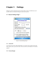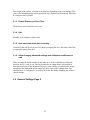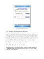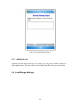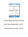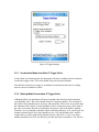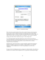
1
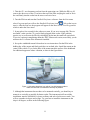
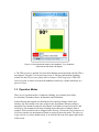
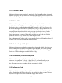
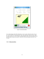
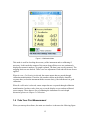
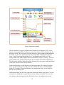
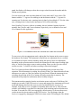
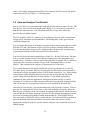
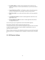
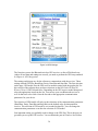
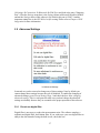
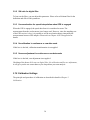
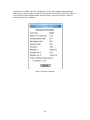
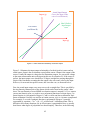
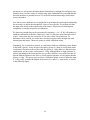
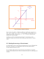
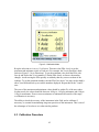
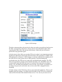
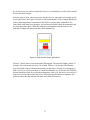
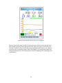
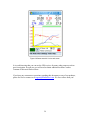
HANDHELD SCIENFITIC, INC. Accelerex User Manual v4.6 11/01/2011 2 Copyright © 2008, 2009, 2010, 2011 Handheld Scientific, Inc. All Rights Reserved 3 4 Safety Warning Start the software and adjust the settings while the vehicle is in complete stop. Never take your eyes off the road when the vehicle is in motion. Never try to adjust the settings or start/stop the software when the vehicle is in motion. 5 6 Table of Contents Chapter 1 Getting Started .............................................................................................. 9 1.1 Software Installation ............................................................................................ 9 1.2 Install Accelerex ................................................................................................. 10 1.3 Operation Modes ................................................................................................ 12 1.3.1 Continuous Mode ........................................................................................ 13 1.3.2 Braking Mode ............................................................................................. 13 1.3.3 Acceleration (Auto Start) Mode.................................................................. 13 1.3.4 Acceleration (Countdown Start) Mode ....................................................... 13 1.3.5 Inclinometer Mode ...................................................................................... 13 1.3.6 Calibration Mode ........................................................................................ 14 1.4 Take Your First Measurement............................................................................ 15 1.5 Save and Analyze Test Results .......................................................................... 18 Chapter 2 Principle of Operation ................................................................................. 21 2.1 Acceleration Sensor............................................................................................ 21 2.2 CompactFlash Plus (CF+) Accelerometer Card ................................................. 22 Chapter 3 3.1 Settings........................................................................................................ 25 General Settings Page 1...................................................................................... 25 3.1.1 Vehicle ID ................................................................................................... 25 3.1.2 Vehicle Weight ........................................................................................... 25 3.1.3 Default Directory to Save Files................................................................... 26 3.1.4 Unit ............................................................................................................. 26 3.1.5 Auto save data when start recording ........................................................... 26 3.1.6 Allow changing advanced settings and calibration coefficients in card ..... 26 3.2 General Settings Page 2...................................................................................... 26 3.2.1 Prompt for User Ready after Zero Adjustment ........................................... 27 3.2.2 Do Not Prompt Confirmation When Exit ................................................... 27 3.2.3 Save Settings on Exit .................................................................................. 28 3.2.4 Prompt on Saving Settings .......................................................................... 28 3.2.5 Save Now .................................................................................................... 28 3.2.6 Load Settings on Startup ............................................................................. 28 3.2.7 Prompt on Loading Settings........................................................................ 28 3.2.8 Load Now.................................................................................................... 28 3.3 General Settings Page 3...................................................................................... 28 3.3.1 Additional note............................................................................................ 29 3.4 Limit/Range Settings .......................................................................................... 29 3.5 Trigger Settings .................................................................................................. 30 3.5.1 Acceleration Mode Auto Start G Trigger Value ......................................... 31 3.5.2 Braking Mode Deceleration G Trigger Value ............................................ 31 3.6 Output Settings ................................................................................................... 32 3.6.1 Do NOT use lateral acceleration for computation in braking mode ........... 32 3.6.2 Use lateral acceleration for computation in all modes ................................ 33 3.6.3 Include X/Y/Z acceleration data in output data files .................................. 33 3.6.4 Generate GPS location and speed and output ............................................. 33 3.7 Compensation Settings ....................................................................................... 33 3.8 GPS Receiver Settings ....................................................................................... 35 3.9 Advanced Settings .............................................................................................. 37 3.9.1 Do not use digital filter ............................................................................... 37 3.9.2 S/N ratio for digital filter ............................................................................ 38 3.9.3 Use acceleration for speed interpolation when GPS is engaged ................. 38 3.9.4 No calibration in continuous or raw data mode .......................................... 38 3.9.5 No zero adjustment in continuous or raw data mode .................................. 38 3.10 Calibration Settings ........................................................................................ 38 Chapter 4 Tire-Surface Friction Coefficients .............................................................. 39 Chapter 5 Calibration................................................................................................... 41 5.1 Principle of Calibration ...................................................................................... 41 5.2 Checking the accuracy of the instrument ........................................................... 44 5.3 Calibration Procedure......................................................................................... 45 Chapter 6 GPS Integration........................................................................................... 49 6.1 Errors in Measurements of Acceleration ............................................................ 49 6.2 The Integration Effect ........................................................................................ 51 6.3 GPS and Accelerometer ..................................................................................... 53 6.4 Setting up PDA to use GPS Receiver................................................................. 55 8 Chapter 1 Getting Started This chapter provides minimum amount of information needed to start using Accelerex. Accelerex Vehicle Performance Test System consists of the following components: Microsoft Windows CE based handheld PDA (for example, HP iPAQ, Dell Axim or TDS Recon) CompactFlash Plus (CF+) Form Factor Accelerometer Plug-in Card Windshield Mount Kit Handheld Performer TM Software Bluetooth Wireless GPS Receiver (Optional) The requirements for handheld PDAs are: having a CompactFlash (CF) expansion slot and running Microsoft Windows CE operating system. Specifically, Pocket PC (PPC) 2003, Windows Mobile 5 and 6 as well as future Windows Mobile versions are supported. However, Pocket PC 2002 or older versions are no longer supported. There are some important differences between Windows CE based handheld PDAs and desktop/laptop PCs. One of them is the power button. For PDAs, the power button is actually a suspension button. When it is pressed, the PDA goes into the suspension mode (or standby mode) where all programs are suspended. To reset the PDA, which like turning off and on the power of a regular desktop/laptop PC, the user needs to stick the stylus to a hole located on the back/side/bottom of the PDA. This terminates all running programs and is usually called software reset. To erase all installed software and return the PDA to the state just out of the factory, you need to perform a hard reset. Look at the user manual of your PDA on how to perform a hard reset. The Handheld Performer software runs on a wide range of PDAs with different hardware. As a result, while the software is running, if the PDA is powered off (suspended) due to idle timeout or manual pressing of the power button, the software may not recover correctly if the power is turned back on again. Therefore, it is highly recommended to re-start the program after the PDA is turned off and then back on. 1.1 Software Installation If you purchased the package with a PDA, the Handheld Performer software should already be pre-installed and you can skip this section. If you accidentally erased the software, or you purchased the package without a PDA, the latest version of the software is always available for download from the company's web site (http://handheldsci.com). It is a good idea to check out the web site from time to time to see if there is a newer version of the software that you can upgrade. Newer versions of the software usually mean more features. The following is a brief description on how to install Handheld Performer software on a PDA. First of all, if you receive a brand new PDA, please read the document coming with it. You will most likely need to install Microsoft ActiveSync software on your PC before connecting the PDA to it. After installing Microsoft ActiveSync on your PC, put the PDA on its cradle and connect the cradle to the PC computer through USB. ActiveSync should detect the device. Follow the instructions on the screen to set up a partnership between the PC and the PDA. The Handheld Performer software requires Microsoft .NET Compact Framework 2.0 which may not be factory installed on some PDAs. Specifically, it is factory installed on Pocket PC/Windows Mobile 6 PDAs but not Pocket PC/Windows Mobile 5 PDAs. If it is not installed, you will need to first install it by yourself. The Framework software package is available from Handheld Scientific’s web site or from Microsoft’s web site. After installing the framework, simply download and install the Handheld Performer software. More detailed instructions are in the download section of Handheld Scientific’s web site. Although not required, before start using Accelerex, change the following settings in your PDA for better user experience: 1. Set PDA to maximum performance: Start Settings System Power Processor and check the box Maximum Performance. This will make sure that the PDA operates at maximum speed. 2. Set longer auto power-off timer: Start Settings System Advanced and set the Turn off device if not used for to 5 minutes. This reduces the chance that the PDA turns itself off during operation due to user inactivity. 3. Set longer display dim timer: Start Settings System Brightness and set the Dim if device is idle for more than to 3 minutes or longer. This reduces the chance that the PDA turns the display off during operation due to user inactivity. Please note all those settings will increase the drain of the battery by a slight amount. However, this is a good tradeoff for enhancing user experience. 1.2 Install Accelerex Follow the following steps: 10 1. Take the CF+ accelerometer card out from the protection case. While the PDA is off, remove the dust cover of the CF socket at the top of the PDA and plug the card in. Press the card firmly into the socket but do not use excessive force. 2. Turn the PDA on and start the Handheld Performer software: from the Start menu select Programs and you will see the Handheld Performer icon . Click on the icon to start it. After the first use, the program will appear in the Most Recent Used Program list which is under the Start menu. 3. It may take a few seconds for the software to start. If you see a message like "Device not found", make sure the CF+ card is firmly plugged in the socket. If the problem persists, try to (soft) reset the PDA by sticking the stylus into the small hole on its back. If you see a message complaining about the .NET Framework version, most likely you do not have the 2.0 version of the framework installed. 4. Set up the windshield mount kit based on its own instructions. Put the PDA in the holding bay of the mount and firmly push the ears on both sides. Install the mount on the center of the vehicle. Try to let the base of the mount touch the surface of the dashboard for additional support to reduce vibration, as show in the figure below. Figure 1-1 Mounting Accelerex in a vehicle. Use inclinometer mode to make sure the PDA is mounted as vertically as possible. 5. Although the instrument does not have to be mounted vertically, you should try to mount it as vertically as possible for better results. The instrument itself can aid the installation: start the Handheld Performer software and select Inclinometer mode. You will see a number in degree and a slope. Try your best to install the instrument so the slope is 90 degree, as show in the following figure. 11 Figure 1-2 Use inclinometer mode to aid installation. Try to install the instrument so the slope is 90 degree. 6. The GPS receiver is optional. For most short braking and acceleration tests the GPS is not engaged. Therefore, it is not necessary to use it. For more information regarding when to use the GPS receiver, please refer to Chapter 6 GPS Integration. If the GPS receiver is used, it can be secured on the dashboard surface by a double-sided tape or a piece of Velcro. 1.3 Operation Modes There are six operation modes: Continuous, Braking, Acceleration (Auto Start), Acceleration (Countdown Start), Inclinometer and Calibration. In the following descriptions we mention the Start and Stop buttons. On the user interface, the Start button is the same widget as the Stop button. When recording is started the Start button becomes the Stop button. In all modes except Inclinometer and Calibration, the instrument will stop recording when either time or distance limit is reached. Those two limits can be changed on the Settings Limit tab. In Inclinometer or Calibration modes, the instrument will start as soon as it enters the mode. The only way to get out of it is to select another mode, or to click the OK icon at the upper right corner of the screen. 12 1.3.1 Continuous Mode In this mode the user starts recording by pressing the Start button. Recording is stopped when the user presses the Stop button (or when one of the stopping limits is reached. This is also true for braking mode and acceleration mode. We will not repeat again). 1.3.2 Braking Mode In this mode the user presses the Start button and accelerates the vehicle to a certain speed then hits the brake. The instrument will begin recording when it detects deceleration value exceeding the threshold which is settable in the Trigger Settings tab. By default, this trigger threshold is a small number (-0.05g) so the instrument will start recording at almost the exact moment when the user hits the brake. The instrument stops recording when it detects the vehicle coming to a stop (acceleration is zero). In ideal condition, when acceleration is zero, speed should also be zero. However, due to error factors (uneven roads, vibration of the vehicle, etc) this may not be the case. But the speed value should be very close to zero, within margin of error. One of the purposes of braking mode is to measure the friction coefficient (drag factor) of a vehicle. This will be discussed further in later sections. 1.3.3 Acceleration (Auto Start) Mode In this mode the user presses the Start button and accelerates the vehicle. The instrument starts recording when acceleration exceeds the trigger threshold, and it stops recording when the user presses the Stop button. The trigger threshold can be set in the Trigger Settings tab. The default trigger threshold value is 0.10g. 1.3.4 Acceleration (Countdown Start) Mode In this mode the user presses the Start button, after the instrument performs zero adjustment, it counts down "2 (beep), 1 (beep), (beep)", and starts recording at the moment when it finishes counting down. The user should start acceleration at the same time. The instrument stops recording with the Stop button is clicked. 1.3.5 Inclinometer Mode In this mode the instrument is used as an inclinometer, i.e., to measure the slope of a surface. Simply place the PDA on the surface, the display will show the slope in degree. A picture of a slope is also shown to make the display more intuitive. 13 Figure 1-3 Inclinometer Mode It is worth pointing out that the inclinometer is more accurate when the angle is close to 90˚. It is less and less accurate (in other words, more and more sensitive to error) when the angle is close to 0˚ or 180˚. Moreover, the orientation of the card socket may not be in precise parallel with the back surface of the PDA so the measurement may not be very accurate. 1.3.6 Calibration Mode 14 Figure 1-4 Calibration Mode This mode is used for checking the accuracy of the instrument and re-calibrating if necessary. In this mode the outputs of the sensor along all three axes are continuously displayed as numeric numbers. No graph is plotted. The data is not saved in memory. The stopping limits are not checked. There is no zero adjustment. Pitch and roll factors are not applied. When Accuracy Verification is selected, the sensor output data are passed through calibration transformation. Therefore, the numbers shown on the display should be accurate data (or what the instrument thinks accurate data), if the instrument is in good calibration. When Re-calibration is selected, sensor output data are not passed through calibration transformation. In other words, what you see on the display are raw and un-calibrated sensor outputs. Those data are for re-calibrating the instrument. For an in-depth discussion, please see Chapter 5 Calibration. 1.4 Take Your First Measurement When you start up the software, the main user interface is shown as the following figure: 15 Tap and Hold for Show/Hide Menu Time Stamp Tap and Hold for Marker Popup Menu Y Axis Zoom-in Main Graph Y Axis Zoom Out Start/Stop Button Clear Button Time Axis Zoom In/Out GPS Switch & Indicator Figure 1-5 Main User Interface The user interface is a typical computer based Graphical User Interface (GUI). At the bottom is the menu bar. The File menu is used to save data to a file or to load a data file previously saved. The Mode menu is used to select one of the operation modes described in Section 1.3. The View menu selects how to view the data. Currently there are three views: Value-Time Graph (the default view), Test Summary and Table view. The Settings menu is for all the settings which are described in Chapter 3 Settings. The Tools menu contains some useful tools such as the Screen Capture tool and the Formula tool. The Help menu contains a link to the online document as well as some useful information (such as the current version) of this software. On the main interface, several display areas have popup menu. To bring up the popup menu, tap and hold the stylus on the area and the menu will show up. For the display fields of G, Latitude G, Speed and Distance, the popup menu allows you to display or hide the corresponding curve. The horizontal strip just above the graph area contains the marker popup menu. You can use marker to calculate the average values between arbitrary two points. To do so, first set a marker at the starting point. After the marker is set, if you tap anywhere on the 16 graph, the display will change to show the average values between the marker and the current cursor position. You can zoom in and zoom out along both the X-axis (time) and Y-axis (value). The buttons with the "+" sign are for zooming in and the buttons with the "-" sign are for zooming out. For the time axis, zooming-in/out is done by the multiple of 2. For the value axis, zooming-in/out is done by the increment of 10% of the total range. Once Handheld Performer software is running, the two hardware buttons which are normally the Calendar and Contacts buttons, respectively, are re-defined as Start and Clear buttons for this application. Start Button Clear Button Figure 1-6 Two hardware buttons are re-defined as the Start and Clear buttons To start a test, select an appropriate mode, and tap the Start button on the screen or press the hardware Start button. The instrument will perform zero adjustment for two seconds. It is essential to keep the vehicle stationary during this period. After zero adjustment, depending on the operation mode selected, the instrument will either start recording right away, or wait for some trigger event to start recording. Please see the Operation Mode section (section 1.3) for how and when recording is started and stopped. The Clear button performs different actions depending on the current state of the operation. If the instrument is recording, the pressing of the Clear button discards all data and starts over again, as if the Start button was just pressed. When the instrument is not recording, the pressing of the Clear button will purge current data in memory. The instrument will prompt for confirmation before actually doing so. The instrument takes samples from the acceleration sensor at the rate of 100 Hertz (100 samples per second). If the GPS receiver is set up and engaged, the instrument will record speed and distance data from the receiver at the rate dictated by the receiver. For example, if the GPS receiver is capable of outputting data at the rate of 10Hz, then the software will faithfully record that. For short tests such as braking and acceleration tests less than 20 seconds, the GPS is not engaged by default setting. So for most those tests, you do not need to turn on and set up the GPS receiver. You can change when the receiver is engaged by changing the GPS kick-in time on the GPS setting tab. The default 17 value is 20 seconds, meaning that the GPS receiver kicks in after 20 seconds. For details on this topic, please see Chapter 6: GPS Integration. 1.5 Save and Analyze Test Results Once a test is done, you can examine the result and save the data in a couple of ways. The first obvious way is to look at the graph on the display. You can zoom-in, zoom-out in both the time and value axes. You can also measure the average value of the data between any two arbitrary points. The Test Summary under View menu gives the summary of the test such as elapsed time, average speed, maximum speed and distance. For braking mode, it also gives friction coefficient (drag factor). You can capture the image on the display using the built-in screen capture tool accessible from the Tools tab. The captured screen is saved as an image in bitmap (BMP) format. You can then upload the images to a PC and import them to almost any word processor or presentation software such as Microsoft Word or PowerPoint. You can also look at the data in tabular form via the View Data Table menu. The data is in 0.1 second (100 ms) interval. Note that the sampling rate of the instrument is 0.01 second (10 ms). Therefore, each row in the table represents 10 samples. The G, latitude G and speed values in each row are the average of the 10 samples in the 0.1 second interval. This is mainly for the purpose of reducing the size of the table. If you would like to have the actual original data in 0.01 second interval, you need to save them via the File menu. Data are saved in plain text files which can be imported to virtually any software for further analysis. The file name extension is ".txt". Most settings of the software under which the data was taken are also saved in the data file for the record. Setting entries in data files all start with the “#” sign which are treated as comments in many software applications. Saving data in plain text files is a major advantage of Accelerex over other similar products that use proprietary format, in which case you also need to use proprietary software to view and analyze the saved data. Once data are saved to files, you can load them back to the Performer software. To do so, go to the File menu and select Load Data. A file chooser dialog will display. Select the data file you would like to load. Once loaded, all settings in the software will be set to the values in the data file. Please note that if you click the Start button attempting to perform a new test, all settings will remain as loaded from the data file. This includes the freeform texts such as vehicle ID, vehicle weight and note. So if you would like to perform a new test unrelated to the data just loaded, you need to make sure you have all the appropriate settings for your new test. Re-start the software if you would like to have all default settings. 18 On the PDA, in File Explorer, when you tap on a saved data file, it is opened in Microsoft Mobile Word because the file extension is .txt. Currently there is no easy way to import data in plain text to Mobile Excel which is pre-installed in many versions of PDAs. However, you can upload the data files to a PC and use Excel to analyze the data there. To do so, establish ActiveSync connection to your PDA. The PDA will appear in the File Explorer on the PC as a directory. Copy the data files over to a folder on your desktop hard drive. Then start Microsoft Excel and import the file to Excel via Data Import External Data. Do not double click on the data files. Doing so will only open the files in Notepad instead of Excel because files with extension .txt are usually associated with Notepad. After you import the data to Excel, open the Insert Chart dialog. In Chart Type, select Line type and any subtype of your choice (the subtype of Line with Markers is a good choice). In the next dialog screen, select Columns for Series in, and select the data range. In most cases you would like to select all data in the data file excluding the lines starting with “#” (setting lines). Click Finish and you will see the graph plotted. From this point on you can change the size of graph, print it out, or embed it in other documents such as a Word document. Excel is one of the most powerful software and you can do sophisticated analysis with it. 19 20 Chapter 2 Principle of Operation This chapter gives more information on how acceleration sensor based instruments work. It helps you better understand and use Accelerex. 2.1 Acceleration Sensor The heart of Accelerex, or most similar instruments in the market, is an acceleration sensor. Those sensors are sophisticated integrated circuits manufactured by advanced technology called MEMS (Micro-Electro-Mechanical System). Only a few large semiconductor companies are capable of making those sensors including Freescale Semiconductor (previously the Motorola semiconductor division), Analog Devices, STMicroelectronics and MEMSIC. The following picture depicts some typical acceleration sensors. Figure 2-1 MEMS Acceleration Sensors from 3 Companies: (1) Freescale Semiconductor (2) MEMSIC (3) Analog Devices Those sensors are quite small: just a few millimeters in size. Different sensors may use different mechanism to measure acceleration but in terms of abstract model, they can all be thought as a mass suspended on springs. When the sensor accelerates, inertial effect causes the change of space between the mass and the surrounding wall. This change of space can be measured by measuring the change of capacitance, or even the change in temperature distribution. Acceleration can then be deducted. The sensors from various manufacturers represent the state of the art of current MEMS technology. Although a particular sensor may perform better in certain aspects, all of them are in the same ball park in terms of major quality parameters such as zero offset, sensitivity variance and temperature coefficient of the sensitivity. The sensors measure acceleration directly. Speed is obtained by integrating acceleration. Distance is obtained by integrating speed. In other words, distance is the second degree integration of acceleration. In discrete time mathematics, the operation of integration is equivalent to summation. It is worth emphasizing that only acceleration is measured directly. Speed and distance, which are really what we care in most cases, are obtained by integrating acceleration. This fact has profound implications to the conditions under which accelerometers can generate reasonable accurate results. Specifically, accelerometers are useful for short tests lasting a few seconds with relatively large acceleration/deceleration during the test period. Otherwise the noise and errors in acceleration measurement will make the results less and less accurate as time goes by. Please see detailed discussion on this subject in Chapter 6 GPS Integration. 2.2 CompactFlash Plus (CF+) Accelerometer Card Accelerex CF+ accelerometer card uses a 3-Axis acceleration sensor from Freescale Semiconductor. The voltage output of the sensor is passed through a hardware low-pass filter to reduce noise. The filtered voltage signal is then fed to an analog-to-digital converter. The digitized data is further filtered by software (digital filter) and displayed on the DPA. 3-Axis Acceleration Sensor Hardware Low-pass Filter AnalogDigital Convertor Digital (Software) Filter Figure 2-2 Function Blocks of Accelerex The sensor has 3 axes (channels) as depicted in the following figure: 22 Display & Record Figure 2-3 Axis Directions The arrows show positive acceleration directions. For example, for the Z-axis (up-down direction), if the PDA accelerates upwards, the output readings for that axis are positive. It is worth noting that the earth's gravity has the effect of acceleration (static acceleration) towards the opposite direction. So if the PDA is positioned upright as shown in the picture, there is a constant 1.00g gravity pulling downwards, this is equivalent to moving the PDA upwards at 1.00g acceleration. So the reading for the Z-axis is 1.00g even if the PDA is not moving at all. This is important to understand especially for calibrating the instrument. 23 24 Chapter 3 Settings Settings are used to control many aspects of the software. They are divided into several sub-tabs which are all under the Setting tab on the main interface. 3.1 General Settings Page 1 Figure 3-1 General Settings Page 1 3.1.1 Vehicle ID A free-form text used for vehicle identification. You can put in any text there such as the make, model, color or year of the vehicle. The text will be saved in data files. This field is optional. 3.1.2 Vehicle Weight The weight of the vehicle, in pound or in kilogram (depending on the Unit setting). This value is for information only and is not used in any calculation at the moment. Therefore, it is alright to leave it blank. 3.1.3 Default Directory to Save Files The directory where data files are saved. 3.1.4 Unit Whether to use English or Metric unit. 3.1.5 Auto save data when start recording If checked, data will be saved to a file without prompting the user. The name of the files is sequential starting from 001. 3.1.6 Allow changing advanced settings and calibration coefficients in card There are some advanced settings for the software as well as calibration coefficients stored in the CF+ card. A user can use the interface to change them, as described in subsequent sections of this document. However, some settings are critical to the proper operation of the instrument and in normal use there is no need to change them. The checkbox here is a safeguard. You need to check this box before changing any of those critical settings. 3.2 General Settings Page 2 26 Figure 3-2 General Settings Page 2 3.2.1 Prompt for User Ready after Zero Adjustment If this box is unchecked (default), then after performing zero adjustment, the software will immediately proceed to the next stage, which is either starting recording or waiting for a trigger depending on the current operation mode. If this box is checked, then after performing zero adjustment, the software will pop up a prompt window and wait for the user to click "OK" before proceeding to the next stage. This allows the user to move the vehicle or do other preparation after zero adjustment. One use scenario is that the spot where you perform zero adjustment is different from the spot where you start your vehicle so you need to move the vehicle after performing zero adjustment, and you want the software to wait while you are moving the vehicle. 3.2.2 Do Not Prompt Confirmation When Exit Each time when you try to terminate the software, it will pop up a dialog box asking for confirmation. This may become unnecessary after some time of use. Checking this box will disable the exit confirmation. 27 3.2.3 Save Settings on Exit If this box is checked, most settings will be saved in persistent storage of your PDA when you exit the program. Note that calibration settings are saved in the CF+ card itself and not in the PDA. Some settings such as "Allow Changing advanced settings and calibration coefficients in card" are not saved because it just does not make sense to do so. 3.2.4 Prompt on Saving Settings Pop up a confirmation dialog to ask you whether you really want to save the settings. Otherwise the Settings will be saved silently if Save Settings on Exit is checked. 3.2.5 Save Now Save settings now. 3.2.6 Load Settings on Startup Load settings from the persistent storage of the PDA each time the software starts up. 3.2.7 Prompt on Loading Settings Pop up a confirmation dialog to ask you whether you really want to load the settings. Otherwise Settings are loaded silently if Load Settings on Startup is enabled. 3.2.8 Load Now Load settings now. 3.3 General Settings Page 3 28 Figure 3-3 General Settings Page 3 3.3.1 Additional note Optional free-form note for the test. For example, you can put the weather condition or road condition here. The note will be saved as part of the file when you save the data. 3.4 Limit/Range Settings 29 Figure 3-4 Limit Settings There are two limit settings: time limit and distance limit. When either limit is reached, the instrument stops recording. This is a way to prevent the software from consuming all resources if, for some reason, it is not able to stop by itself (such as in braking mode) or the user fails to hit the stop button (such as in acceleration mode). There are also two range settings: speed range and acceleration range. Speed range only affects the display of the graph. Acceleration range has four selections: 1.5g, 2.0g, 4.0g and 6.0g with 1.5g being the default. The instrument is calibrated in factory for 1.5g. Using any other range will require re-calibration of the instrument. 3.5 Trigger Settings Currently there are two trigger settings: Acceleration Mode Auto Start G Trigger and Braking Mode Deceleration G Trigger as described below. 30 Figure 3-5 Trigger Settings 3.5.1 Acceleration Mode Auto Start G Trigger Value In Auto Start Acceleration mode, the instrument will start recording when acceleration reaches this trigger value. This value should always be a positive number. Note that this value does not apply to countdown acceleration mode where recording starts as soon as countdown is done. 3.5.2 Braking Mode Deceleration G Trigger Value In Braking Mode, the instrument will start recording when it detects the deceleration exceeding this value. This value should always be a negative number. The selection of this value is the tradeoff between accuracy and sensitivity. If this value is too small, then the vibration of the vehicle or road conditions such as a bump may cause a false start. If the value is too large, then the recording does not start as soon as the brake is applied. Therefore, for very smooth road and a vehicle with little vibration, -0.01 can be used. For normal road and vehicle, this value should be set to -0.05 (the default value). And for rough road or a vehicle with strong vibration such as a big truck, -0.10 or even large number should be used. The user interface provides three pre-set numbers. You can also 31 use a custom number. In such case please note that the negative sign is outside of the input box. So you should type in just a number without the negative sign. The software will add the negative sign to make it a negative number. 3.6 Output Settings There are four settings on this tab which are all checkboxes. Figure 3-6 Output Settings 3.6.1 Do NOT use lateral acceleration for computation in braking mode During hard braking tests, a vehicle can rotate (yaw) while it is sliding. To measure the full deceleration in those tests, lateral (Y-Axis, or left-right) deceleration is combined with longitudinal (X-Axis, or back-forth) deceleration to more accurately compute speed and distance. The combined value is sqrt(Gx2 + Gy2) where sqrt is the square root function and Gx, Gy are the X axis and Y axis deceleration, respectively. This is recommended for all braking tests and is the default setting. However, if you do not wish to use lateral deceleration in computation, check this box. 32 3.6.2 Use lateral acceleration for computation in all modes In all modes except braking mode, only longitudinal acceleration is used to compute speed and distance. Lateral acceleration is not used. However, you can instruct the software to use lateral acceleration by checking this box. When lateral acceleration is used, the combination formula is the same as in braking mode described above. 3.6.3 Include X/Y/Z acceleration data in output data files If you check this box, acceleration data along all three axes will be included in the output data file so you can do your own analysis. Zero adjustment values are also saved in the file. It is worth noting that calibration, zero adjustment and pitch/roll factors have all been applied to the raw x/y/z acceleration values before they are written out to files. 3.6.4 Generate GPS location and speed and output If you check this box, and if GPS is used and kicked in, then the GPS location and speed values will be recorded in data files. Therefore, the instrument can be used as a GPS data logger. However, logging GPS data for long time (more than a few minutes) is not recommended since this is not the purpose of the instrument. 3.7 Compensation Settings 33 Figure 3-7 Compensation Settings Pitch is the front-to-back tilt and roll is the side-to-side tilt. Because of the suspension system, when a vehicle is in hard acceleration or braking, pitch and roll may change. Depending on the type of vehicle, the change can range from none to relatively large. To obtain accurate results, such change must be accounted for. This is done by manually setting a pitch and roll factor based on the type of vehicle being tested. It is worth noting that the pitch and roll factors here refer to the dynamic tilt due to suspension shift under acceleration and deceleration. They do not refer to the static tilt of the vehicle or the unevenness of the ground, as any such static factor is already compensated by zero adjustment. Mathematically, pitch and roll factor are simply multipliers applied to the longitude or latitude G calculation, respectively. For instance, if the pitch factor is 0.97, then the longitude G will be multiplied by 0.97 before being displayed or used for other calculations. For most vehicles including motorcycles, passenger cars and semi trailers, the pitch factor should be set to normal, which is adjusted to 0.970. In general the following rules apply: 34 Low Pitch (1.000): for vehicles with no suspension such as transit rail cars, forklifts or farm tractors. Also for normal vehicles on very low friction surfaces such as ice. Normal Pitch Factor (0.970): for all highway vehicles with useful suspension systems, including motorcycles, passenger cars and semi tractor-trailers. High Pitch (0.940): for very short wheel based vehicles with a long suspension travel. Very High Pitch (0.910): for marine or similar application when the bow rises higher than the stern. Extreme High Pitch (0.880): for marine or similar application when the bow rises higher than the stern. You can also type in your own pitch factor in the custom number input box. The roll factor should be 1.000 for all practical purposes because acceleration/deceleration in the forward direction should not affect the side-to-side tilt of a vehicle. Nevertheless, this factor is made available for modification so users can experiment with it if so desired. Those two factors can also be used to adjust the results for any reason. Just keep in mind that the pitch factor is a multiplying factor for longitude G and the roll factor for latitude G. 3.8 GPS Receiver Settings 35 Figure 3-8 GPS Settings The first time you use the Bluetooth wireless GPS receiver, or after a PDA hard reset (where all user data and settings are erased), you need to perform the GPS setup outlined in Chapter 6: GPS Integration. The settings on this page are for the software to communicate with the receiver. Those settings include GPS Port, Baud Rate, Parity, Data Bits and Stop Bits. The first selection on the page, GPS model, lists the GPS receiver models coming with the product kit. For this version of the software there are three selections on the list: Holux GPSlim236, Wintec G-Rays I WBT 300 and Other. Depending on the GPS receiver model being used, select the appropriate item from the list. You can use your own Bluetooth receiver as well. In that case select Other from the list and set the appropriate communication parameters for your device. The selection of GPS model will only set the selections of the communication parameters (Baud Rate, Parity, Data Bits and Stop Bits) to the default value for that particular receiver. The selection of GPS model is not recorded in data file. You can change the communication parameters even after the selection of GPS model. One important setting you probably need to change is the GPS Port. This is the port you got when you set up the GPS receiver. You can obtain the port in Windows Start Button 36 Settings Connections Bluetooth COM Ports and look at the entry "Outgoing Port". (Note the Settings menu here is the Settings Menu in Microsoft Windows Mobile and not the Settings menu of this software). By default, this port is COM7. Another important setting here is the GPS Kicks In After setting. Please refer to Chapter 6 GPS Integration for more information. 3.9 Advanced Settings 3-9 Advanced Settings In normal use you do not need to change any of those settings. Note by default you cannot change those settings because they are all disabled. To enable the changing of advanced settings, go to General Settings Page 1 and check the box Allow changing advanced settings. This is a safe guard to make sure you don't change the advanced settings accidentally because they are essential to the proper operation of the software. 3.9.1 Do not use digital filter Digital filter is necessary to reduce the measurement noise. The software employs a sophisticated digital filter, the Kalman filter. If you wish to use your own digital filter to analyze the data instead of using the built-in one, check this box. 37 3.9.2 S/N ratio for digital filter To best use the filter, you can adjust this parameter. Please refer to Kalman filter for the definition and effect of this parameter. 3.9.3 Use acceleration for speed interpolation when GPS is engaged When the GPS is engaged, the speed data from it is considered accurate. The measurement from the accelerometer is no longer used. However, since the sampling rate of the GPS receiver is low, it is possible to use the acceleration data to interpolate the measurements between GPS samples. Please refer to Chapter 6 GPS Integration for details. 3.9.4 No calibration in continuous or raw data mode If this box is checked, calibration transformation is not applied. 3.9.5 No zero adjustment in continuous or raw data mode If this box is checked, zero adjustment is not applied. Checking of the boxes of Do not use digital filter, No calibration and No zero adjustment, it will give you the raw sensor data so you can perform your own analysis. 3.10 Calibration Settings The principle and procedure of calibration are described in detail in Chapter 5: Calibration. 38 Chapter 4 Tire-Surface Friction Coefficients Accelerex can be used to obtain tire-surface friction coefficient. This chapter gives some general information on the subject. The friction of a tire against the road surface is given by the tire-surface friction coefficient (Greek letter). Practically there are three ways to determine the value of . 1. Table: tables give tire-surface friction coefficients by types of road surface and the condition of those surfaces. The book Equation Directory for the Reconstructionist by Daniel J. Parkka has such a table. Tables will generally have a rather large range of values for any given surface and condition. Since we often do not know the circumstances of the testing procedure, we do not know specifically how a particular test corresponds to the circumstances of the crash under study so tables usually have limited use. 2. Drag Sled: a drag sled is a piece of tire filled with heavy substance like cement. The tire is then weighted and pulled along the road surface. The force needed to pull the drag sled is measured. The friction coefficient is then calculated by using the following formula: = F / W, where F is the pulling force and W is the weight of the tire. However, drag sleds do not take into account the aerodynamics of a vehicle, which will substantially affect the results. 3. Skid Test: accelerate the vehicle to a certain speed (say, 30 mph) then apply the brake as firmly as possible to lock the wheels and make the vehicle skid. The distance of the skid is then measured. The friction coefficient is calculated using = s^2 / (30 * d) where s is the speed (in mph) when the brake is applied and d is the distance of the skid (in feet). If metric system is used, the formula becomes = s^2/(254*d) where speed is in kph (kilometers per hour) and distance is in meter. The skid test method is the preferred one since it accounts for the aerodynamic property of the vehicle under investigation. Accelerex can be used to obtain tire-surface friction coefficients. It uses the skid test formula to compute the coefficient. After a braking test, the coefficient is available under View Test Summary, as shown in the following figure. Please note that the friction coefficient is available only after a braking test. It is worth emphasizing that during a braking test, you must apply as much force as possible on the brake to lock the wheels so as to generate reliable measurements. In other words, you need to skid the vehicle to measure the friction coefficient. Figure 4-1 Friction Coefficient 40 Chapter 5 Calibration 5.1 Principle of Calibration As with any sensitive measurement tool, calibration is a very important factor in getting accurate results, especially for sensor based instruments. There are several reasons for calibration, such as environment changes especially temperature change, the aging of the sensors, and the effect of large vibration during transportation of the device. Those factors may all potentially change the characteristics of the sensor, making re-calibration necessary. Essentially, an acceleration sensor is a mass suspended on springs, so it is not hard to imagine that such devices can’t maintain the same characteristics forever. For instance, even when the sensor is sitting still, one of the springs is compressed and some others are extended due to the weight of the mass. For long period of time the characteristics of the springs may change, therefore affect the parameters of the sensor. Inside Accelerex, there are other components that may contribute to errors besides the sensor. Those components include hardware filter, analog-digital converter and digital (software) filter. However, compared to the sensor, errors introduced by other components are very small and can be ignored. Therefore, in the following discussion, we will focus on the error introduced by the sensor and how to correct it. There are two major parameters related to the error of an acceleration sensor: zero offset and sensitivity coefficient. Zero offset is the output of the sensor when acceleration is zero, and sensitivity is the ratio of output versus input. If the sensor is perfect, zero offset should be zero and sensitivity should be one (after normalization). However, in reality, those two parameters may differ from their ideal value significantly. Output (g) Actual Input/Output Curve (the slope of the curve is coefficient A) Ideal (Perfect) input/output curve Zero Offset (coefficient B) Input (g) Figure 5-1 Zero Offset and Sensitivity of Sensor Output Figure 5-1 illustrates the input-output relationship of an ideal (perfect) sensor and an actual sensor. Input is the acceleration erected on the sensor. Output is the output of the sensor. Usually the output is voltage but for illustration purpose, we convert the voltage to the same measurement unit as the input (in this case acceleration G). If the sensor is perfect, the input-output curve should be a 45 degree straight line passing through the origin of the coordinates, meaning that the output is the exact same value as the input. However, for an actual non-perfect sensor, this is not the case, as discussed below. First, the actual input-output curve may not even be a straight line. This is specified by the non-linearity characteristic of the sensor which can be found on the sensor’s data sheet. The non-linearity of most MEMS acceleration sensors is around 1%. If we want to correct non-linearity error, we need to use a polynomial function of at least degree 2 (a linear function is a polynomial of degree 1), and we call it non-linear calibration. Nonlinear calibration is usually not used for two main reasons: (a) it is a lot more complicated. For example, if we used a quadratic function (a polynomial of degree 2 generally represented by equation y = Ax2 + Bx + C), we then need 3 calibration points. This is difficult to do in many situations; (b) its effectiveness is questionable since we usually don’t know what degree of polynomial we should employ. Therefore, in the following 42 discussion, we will assume the input-output relationship is a straight line and ignore nonlinearity errors. In other words, we will use only linear calibration. Keep in mind that this decision introduces a potential error of 1% of the full measurement range, based on the sensor’s datasheet. Now that we have decided to use a straight line to proximate the input-output relationship, the next task is to define that straight line. Once we have the line, we can then calculate the input value based on the output value of the sensor. The process of obtaining that straight line is actually the process of calibration. We know any straight line can be represented by equation y = Ax + B. We call numbers A and B the calibration coefficients. Intuitively, value A is the slope of the line and value B is the Y value where the line crosses the Y axis (also called Y-axis intersect). To determine values A and B, we need to have at least two points on the straight line with known input and output. Those two points are called calibration points. Fortunately, for accelerometer sensors, it is not hard to find two calibration points, thanks to the earth’s gravity. As we all know, the earth’s gravity is a form of acceleration (static acceleration). On most surface of the earth, the gravity is 1.00g. When we flip the sensor upside down, we have static acceleration of -1.00g. Although there is slight variation of gravity depending on the location where we are, this variation is very small (less than 0.5 percent from the Equator to the Pole) so for all practical purposes we can assume that the gravity is 1.00g. The gravity gives us the two calibration points we need. When the input is -1.00g/1.00g, we name the outputs of the sensor Gmin and Gmax, respectively, as shown in the following figure. 43 Actual Input/Output Line Output (g) Gmax -1.00g 1.00g Input (g) Gmin Figure 5-2 Determine Calibration Coefficients Once we know Gmin and Gmax, calibration coefficients A and B can be computed as A = (Gmax – Gmin) / 2 and B = (Gmax + Gmin) / 2. So for any output y from the sensor, we can compute the true input x using formula x = (y – B) / A. The value x obtained by this formula is the calibrated output. Coefficients A and B are obtained and stored in the CF+ card in factory. In the Calibration Settings screen, you can see the coefficients as well as the Gmax and Gmin values. 5.2 Checking the accuracy of the instrument As described above, due to several factors, the instrument may be out of calibration from time to time. Therefore, it is recommended to check its accuracy before each use. Accelerex makes this check very easy. As we recall, the earth’s gravity is an accurate source of acceleration. To verify the accuracy of the instrument, select Calibration from the Mode menu. The following screen is shown: 44 Figure 5-3 Calibration Mode Keep the selection at Accuracy Verification. Then move the PDA slowly to get the maximum and minimum values of each axis. For example, the X axis direction is backforth (see Figure 2-3 Axis Directions). To get the minimum value, hold the PDA with face up and look at the X Axis number. Turn the PDA slowly to observe the number changes. Avoid moving the PDA quickly or suddenly that may cause overshoot of the readings. To get the maximum number, turn the PDA face down. You may need to hold it above your head and look up to read the numbers displayed. Repeat this for the Y and Z axes. The error of the maximum and minimum values should be within 2% of the true values. In other words, the values should be between -0.98g to -1.02g for minimums and 0.98g to 1.02g for maximums. If one or more maximums or minimums fall outside of the range, re-calibration is necessary. The ability to check the accuracy of the instrument in the field, and re-calibrate if necessary, is essential in maintaining long-term precision of the instrument. This is one of the advantages of Accelerex over other similar products. 5.3 Calibration Procedure 45 Caution: Saving new calibration coefficients to the CF+ accelerometer card will replace the data previously stored there. Make sure you understand the calibration procedure before doing so. When Accelerex fails accuracy verification, re-calibration is needed. Thanks to the carefully designed software, re-calibration can easily be done. The procedure involves two steps: (1) find the un-calibrated minimum and maximum values, (2) Use the Calibration Settings interface to compute and save calibration coefficients. The procedure is done for each channel that is found out of calibration. In the following description, we will use the X channel as an example. Step 1: find the un-calibrated minimum and maximum values. In Calibration Mode as shown in Figure 5-3, select Re-calibration. When this selection is made, the data shown is the un-calibrated raw data from the sensor. Like checking accuracy, turn the PDA slowly to get the maximum and minimum values. Those values could differ from ±1.00g by as much as 25% or even more. As an example, for a particular card, the minimum is found -1.08 and maximum 0.96. Write down the values and repeat this for all axes needed to recalibrate. Step 2: use the Calibration Settings interface to compute and save calibration coefficients, as shown in the following figure. Calibration Step 2-1 Select a Channel Calibration Step 2-2 Type in the min and max numbers found in step 1. Calibration Step 2-3 Click this button. The value in A and B should be updated accordingly. Calibration Step 2-4 Click this button. A dialog box will show to confirm that the values are saved. Repeat for all channels. Figure 5-4 Illustration of Calibration Step 2 46 Select the appropriate axis (channel). You will see the minimum and maximum values as well as the calibration coefficients already filled in. Those are the values currently stored in the card. Now change the minimum and maximum values you obtained in the previous step. It is worth noting that the minimum is always a negative number and the maximum a positive number. Usually the new value should be close to the old one because the characteristics of the sensor should not change that much. If a new value is substantially different from the old one, you should double check to make sure you did it right in the previous step. After inputting the minimum and maximum values, click the Compute Coefficients button. You should see the A and B values changed accordingly. The value A should be a number close to 1 and the value B should be a number close to zero. If all numbers look good, click the Save Coefficients to Card button. The coefficients will then be saved to the card, replacing the old values. Please note that the Save Coefficients to Card button is normally disabled to prevent accidental overwriting. You need to check the box Allow Changing advanced Settings and Calibration Coefficients in Card on General Settings Page 1 (see Section 3.1 General Settings Page 1) to enable this button. You can also type in the coefficient A and B directly without using the minimum and maximum for calculation. As evident in the previous discussion, the A/B values the min/max values are mutually dependent. In other words, knowing either pair can deduct the other. So if you directly type in values A and B, chances are that they are not consistent with the min/max pair. In such case the software will pop up a confirmation dialog making sure that you really want to use the A/B values you typed in and ignore the min/max values. The calibration coefficients are stored in the CF+ card itself (not in the PDA), so you can move the card to a different PDA without the need to re-calibrate. After re-calibration is completed, repeat calibration verification. If all have been done correctly, verification should pass this time. 47 48 Chapter 6 GPS Integration This chapter explains the conditions under which acceleration sensor based instruments (accelerometers) are appropriate in measuring speed and distance, and the rationale to add a GPS receiver to Accelerex. You can skip the first two sections if you are not interested in theoretical discussion. The principle of accelerometer-based instruments is simple: when placed inside a vehicle they measure the vehicle’s acceleration (the rate of change in speed) and compute speed and distance based solely on acceleration. In theory, once you know the acceleration and the starting values of speed and distance (both of them start from zero in practice), you can accurately determine them at any point of time by integration (or by summation in discrete time). But in reality, what are the issues of doing such? There are two main issues: The error of acceleration measurements, and The effect of acceleration measurement error to the speed and distance calculation. Let's look into those two issues more closely. 6.1 Errors in Acceleration Measurements As in measuring any physical quantity, the measurements of acceleration are not without error. There are a number of sources causing measurement error including vibration, uneven road and the error of the instrument itself. When a vehicle is in motion, vibration can be large. Vibration may be caused by road condition, the engine and any moving parts of the vehicle. Vibration can be measured by simply driving the vehicle at constant speed and measure its acceleration in all axes. Empirical data show that even for passenger cars on smooth road, the equivalent acceleration caused by vibration can be as large as 0.1g. This value could be a lot larger for trucks or on rough road. For most small cars, when they are in hard acceleration, the average acceleration is around +0.3g to +0.6g. When in hard braking the average deceleration is from -0.5g to 1.0g. As you can see the error caused by vibration can be more than 10% of the real acceleration value. The Figure 6-1 below shows the acceleration/braking measurement of an average passenger car on a common city road. The red line is the raw measurement data and the green line is the estimates of the acceleration using advanced digital filter techniques. The vibration level may more or less depend on the type of vehicles, the road condition and the vehicle's speed, etc. But it is clear that the vibration level can be relatively large comparing to the actual acceleration we would like to measure. It is hard to know what the real acceleration value is so everything is just an estimate using various filter techniques. That is why if you use different brand of acceleration sensor instruments to measure identical testing runs, the results could be slightly different. This is because different instruments use different filter algorithm, thus generate different results. Figure 6-1 Raw Measurement and Estimate of a Normal Acceleration/deceleration Test It is worth noting that using a “better” sensor cannot eliminate noise. The vibration is real. It is not because of the sensor. The sensor itself has no way to distinguish the acceleration caused by vibration from that caused by the car’s movement. The only way to separate them is to use a filter (either hardware or software) based on the fact that the acceleration caused by vehicle’s movement changes slower than that caused by vibration. In technical terms, we call slowly changing quantity low frequency and fast changing quantity high frequency, and we use a low-pass filter to eliminate high frequency portion of the signal. Uneven road is another error source. During zero adjustment, any road leveling factor is measured and accounted for. However, this is just for the location where zero adjustment is preformed. Once the vehicle starts moving, the road leveling condition has now changed since the location has changed. This also introduces measurement errors. There are other factors such as the errors in the sensor itself and the pitch/roll factors. Understandably, nothing is perfect and there are always measurement errors. However, as you will see in the following section, such errors have profound implications in the accuracy of the instrument especially in the calculation of speed and distance values. 50 6.2 The Integration Effect Once we have the acceleration measurements, speed can be obtained by integrating acceleration, and distance can be obtained by integrating speed (i.e., second degree integration of acceleration). However, integration has one very important effect: any error in acceleration measurement will cause permanent error in speed and distance calculation. It is like integration "remembers" everything happened in the past. The following three figures illustrate this effect. Those figures are generated by computer simulation to illustrate the point. Figure 6-2 Acceleration versus Time The figure above shows acceleration. The red curve and the green curve are two simulated measurements. Those two curves are identical most of the time (so only the green curve is shown most of the time because the red line is underneath it). The only exception is around time=1 where the red curve has a small jump representing some measurement error resulting from things like a small bump on the road. 51 Figure 6-3 Speed versus Time Figure 6-3 shows speed which is the integration of acceleration. One can see after the measurement error at t=1, two speed curves differ from that point on, even if there is no error in acceleration measurement after that. This is because integration has the property of "remembering" all events in the past including the occurrence of the error at time t=1. Figure 6-4 Distance versus Time Figure 6-4 shows the distance which is the integration of speed (or the second degree integration of acceleration). The situation is now worse. The difference not only exists permanently but also increases over time! This is because the error in speed is "adding up" in distance. 52 From those 3 figures one can see that even an isolated, short-lived error in acceleration measurement can cause permanent error in speed and distance, and the error increases over time in the later case. This is the inherent property of integration. To summarize what we have just discussed: because of vibration and other factors, acceleration measurements contain errors. Because of integration effect, speed and distance results can be even worse, and errors increase over time. Therefore, those instruments based solely on acceleration sensors are hard to get accurate results over relative longer time period (greater than a few seconds). The shorter the time interval, the more accurate they are. Another condition to use accelerometers is that the acceleration during the test period should be relatively large. To see why, let’s assume that the error caused by all the factors such as vibration is equivalent to 0.05g. If the average acceleration during the test period is 0.50g, then the error is 10%. However, if the average acceleration during the test period is low, like only 0.10g, then the error is now 50% of the measurement! This is why accelerometers are used for hard acceleration and braking tests where average acceleration is at least 0.4g. And you can only do short tests lasting a few seconds. As a result, longer tests like accelerate-cruise-brake will not generate accurate data. It is worth pointing out that the integration effect is not always bad. For instance, if vibration is perfectly symmetric (it goes up and down by roughly the same amount around a fixed value) then integration effect can actually alleviate the error by canceling out the deviations. However, in reality vibration especially that caused by road conditions is not symmetric. Errors caused by sources like uneven road, sensitivity variance and pitch/roll factors are certainly not symmetric. They will cause the accumulation of error in speed and distance very quickly over time. As you can see from the above discussion, acceleration sensor based instruments are good only for short test lasting for a few seconds. During the test period there should be relatively large acceleration/deceleration so as to reduce the effects of noise. If you let instrument run for longer time, the errors will quickly cumulate, making the output reading less and less accurate as time goes by. 6.3 GPS and Accelerometer GPS (Global Positioning System) receivers can accurately measure both speed and distance. Those receivers typically calculate speed by measuring the frequency shift (Doppler shift) of the GPS D-band carriers. Therefore, the measurement is very accurate. For speed, they can achieve 0.1 meter/s (0.22 miles/hour) accuracy. If you travel along a straight line, distance measurement is also very accurate, usually within 3-5 meters. It is also important to note that unlike acceleration based instruments which employ integration, the accuracy of speed and distance measurements of GPS does not change over time. 53 However, there is one major issue in using GPS to measure vehicle performance: most low-cost GPS receivers in the market only update data once every second (1 Hertz, or 1Hz). A few receivers can go up to 10Hz. This is in large part due to the intense computation required to generate one data output. In vehicle acceleration/braking tests where speed changes rapidly, it usually requires 100 samples per second to record all the dynamics. So the 1Hz or even 10Hz sampling rate of most GPS receivers falls short of meeting that requirement. As such, GPS is good only for long tests where slower sampling rate is adequate. As we remember, accelerometers are appropriate for short tests, and GPS receivers are appropriate for long tests, so if we combine those two together, wouldn’t that make the instrument useful in a lot more situations? This is exactly what Accelerex is designed to do. The integration of accelerometer and GPS receiver is another advantage of Accelerex over other similar products. For Accelerex, when GPS is engaged, speed and distance values from it are viewed as reliable. In other words, speed and distance calculated by integrating acceleration are no longer used. Since the data update rate of the GPS receiver is low, you will see flat lines for a period, and they jump to a different level for the next period. One period is the time between data updates. For 1Hz GPS, it is one second. For 10Hz GPS, it is 0.1 second. When GPS is engaged, since the upgrade rate is much slower than that of the acceleration sensor, it is suggested to use acceleration data to obtain more accurate speed and distance values by using interpolation technique as the following: suppose at time t, the speed is s, and the acceleration is assumed as constant a, then at time t+0.01 (where 0.01 is the sampling period for the acceleration sensor), the speed is then s+0.01*a because its change during that 0.01 second is 0.01*a. Using this algorithm, one can indeed obtain a more smooth speed and distance curves. In the Advanced Settings of the software, there is a setting Use Acceleration for Adjustment when GPS is Engaged. Checking this box will enable acceleration adjustment as explained. However, whether this algorithm actually increases the accuracy of the data is in question. The main reason is that we do not know exactly what the GPS speed data represent. When it outputs a speed value at time t, we do not know whether this is the instantaneous speed at exactly time t, or at time t minus one sampling period, or at any point in between. The best interpretation is that this value is the average speed during the past sampling period. So it is not certain that the interpolation algorithm described above improves the accuracy during that one sampling period when the base value is an average. As such, the default behavior is not to use the acceleration adjustment algorithm. This actually makes the curve easier to understand. See a test example in a later section of this document. 54 6.4 Setting up PDA to use GPS Receiver First of all, please read the manual of the Bluetooth GPS receiver. Then follow the procedure below to set up your PDA to use the GPS receiver. This needs to be done only the first time you use it. 1. Switch on the Bluetooth GPS receiver. If you just got it, you may need to charge the battery first. 2. Turn on Bluetooth wireless on PDA: Settings Connections Bluetooth, check the Turn on Bluetooth box. Note the Settings menu here is the Windows setting menu not the Handheld Performer software Settings menu. Now click on the Devices tab and then New Partnership, the PDA will now search for Bluetooth devices in range. When it is done, you should see HOLUX GPSlim236 (or G-Rays1, or some other name if you use another brand of GPS receiver) on the list. Select that device and then click Next. Enter pass code "0000" (factory default for all devices), then click Next. You will see Serial Port on the service list. Check the box, and click Finish. Now click the COM Ports tab and select New Outgoing Port. Select HOLUX GPSlim236 (or G-Ray1) on the next screen and click Next. On the next screen, select the port COM7 (the default) and uncheck the Secure Connection box (this is very important!). Now on the COM Port List, you should see HOLUX GPSlim236 (COM7) or G-Rays1 (COM7). To test the setup, start Handheld Performer software, go to Settings GPS tab (see below) and click the Test GPS button. It should come back without an error message. 55 Figure 6-5 GPS Settings The above setup procedure only needs to be done once unless you perform a hard reset on the PDA. If you perform a hard reset, all user software and configuration data will be erased and the PDA will be like just out of the factory. In this case you will need to perform the setup procedure again. After the setup is done, before you use the GPS receiver, there is one important parameter needed to be understood, which is the GPS kick-in time. This parameter is settable on the GPS Setting tab (see Figure 6-5 GPS Settings). As already explained, the sampling rate of the GPS receiver is slow (from 1Hz to 10Hz), therefore, for short braking and acceleration tests, the GPS receiver is not useful, and should not be engaged. The GPS kick-in time parameter specifies when GPS data should be used. The default value is 20 seconds which means that GPS data won’t be used until 20 seconds after recording is started. You can change this parameter to suit your tests. For example, if you know you are doing a long test, you can set this value to zero so the GPS is engaged from the beginning. All other settings on the GPS Settings tab are pretty much self-explanatory. Those are all standard serial port settings. You simply select the model of the GPS receiver and all the values will be selected for the defaults of that receiver. You can use your own receiver 56 too. In such case you need to consult the receiver’s user manual to see what values should be used for those settings. After the setup is done, when you want to use the receiver, tap on the red rectangle on the lower right corner (see Figure 6-6 below) of the main interface. The rectangle should turn yellow, indicating that the connection to the GPS receiver has been established. If it comes back with some error messages, you will need to double check the parameters and the setup procedure above. When the software is getting data from the receiver, the indicator rectangle will turn green and yellow alternatively. Figure 6-6 GPS Receiver Button and Indicator Figure 6-7 below shows a test result with GPS engaged. The total test length is about 30 seconds. The kick-in time was set to 10 seconds. Before t=10, the speed and distance were calculated using acceleration integration. At and after t=10, they were obtained via GPS receiver. As you can see, there is a small discontinuity at t=10 because the GPS data did not match the results by acceleration integration. After t=10, the curves are a series of jumps once per second because that is how frequently the GPS data were updated. The green bar above the data indicates the data came from GPS receiver. 57 Figure 6-7 A test with GPS kick-in time set to 10 seconds. Figure 6-8 shows the same test with 1:8 time axis zoom. In other words, one data point on the graph represents 8 actual data points so the whole test can be viewed all at once. You can see that the vehicle accelerated, cruised, and then braked. Again, you cannot do such tests using accelerometer alone. With GPS engaged, you can do much longer tests lasting minutes and miles. This illustrates the values of combining GPS technology with accelerometer. 58 Figure 6-8 Same test with 1:8 time axis zoom It is worth knowing that you can use the GPS receiver for many other purposes such as travel navigation. In such case you will need to obtain additional software such as Tomtom or Microsoft Pocket Street. If you have any comments or questions regarding this document, or any of our products, please feel free to contact us at [email protected]. We love to hear from you! 59