Download User`s Manual for CNAG (Copy Number Analyser for GeneChip

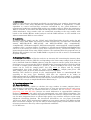
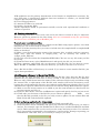
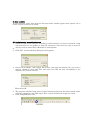
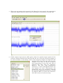
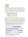
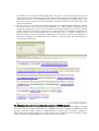
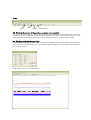
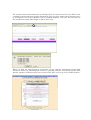
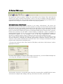
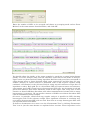
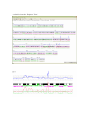
User’s Manual for CNAG (Copy Number Analyser for GeneChip®)
Ver. 1.1
1. Introduction
CNAG is the software developed specifically for analyzing copy number alterations and
LOH in cancer cells using Affymetrix® GeneChip® platform. It implements a robust
algorithm to correct between-chip variations introduced by the subtle difference in
experimental conditions, enabling high quality copy number analysis. When the constitutive
DNA is available, it also allows for allele-based copy number estimation to sensitively detect
allelic imbalances. Copy number calls are automated according to the copy number calls
based on the hidden Markov model analysis and the LOH inference is also enabled even
when constitutional DNA is not available.
2. Installation
To install CNAG, simply put the ‘CNAG’ and ‘CNAGView’folders directly under the ¥C
directory. The CNAG folder will contain a CNAG excutable file, and other files and folders
named, ‘MSVCR71D.dll’, ‘MFC71D.dll’, and ‘MSVCP71D.DLL’ files, ‘sampledataX’,
‘sampledataH’, ‘SNPtumorsampleX’, ‘SNPtumorsampleH’, ‘tumorsampleX’, ‘tumorsampleH’,
‘temporary files’, and ‘data’ folders. In addition, it should contain XbaRef and HindRef files
and if it is not found you need to create these reference files by yourself according to the
instruction described below using CNAG software. We confirmed that this program runs on
Windows XP and 2000. At least 512Mb RAM is required, but 1Gb or more is recommended
for quick response.
3. Preparing Data files
CNAG requires two kinds of files for analysis, an ‘intensity file’ containing the intensity data
of all SNP probes, and the ‘SNP file’ corresponding to the same tumor sample, both of which
can be obtained from the GDAS® software using the ‘export to txt file’ option. Note that you
should not sort or rearrange the SNPs in GDAS® before exporting the data. Each file should
be saved as ‘sample_name’ followed by ‘_X.txt’ or ‘_H.txt’ according to the array used. Any
names can be used for ‘sample_name’, but they must be unique and we strongly
recommended that both should be easily linked together. ‘sample_name_X.txt’ and
‘SNP_sample_name_X.txt’ for files from Xba arrays are examples.
Intensity files should be placed in the tumorsampleX folder or tumorSampleH files
according to the array type. Similarly, SNP files are expected to be either in
SNPtumorsampeleX or SNPtumorsampleH folder. If a self-reference sample is available,
both intensity file and SNP file for the self-reference should be placed into the sampledataX
folder (for Xba arrays) or sampledataH folder (Hind arrays).
4. Createing reference files
4.1. Recommendation
‘Ref ’ files are used by CNAG to calculate the copy number in tumor samples when a
self-reference is unavailable and you must have at least one reference file for each array
(Xba or Hind). You may use attached Ref files if available, but we strongly recommend
preparing your own Ref files, because too much differences in experimental conditions
(between one lab and the other) will not compensated even with CNAG algorithms. You
should understand that uniform experimental conditions between samples and references
are the most important factor to obtain high quality copy number analysis results using
Affymetric GeneChip platform. For theoretical discussions, see our paper (CancerRes
10(14):1-10, 2005). If the experimental condition of your tumor sample is too different from
those of reference samples, you are not likely to obtain high quality results. Below is the list
of known parameters that may affect experimental conditions:
(1) PCR devices
PCR conditions are the primary determinant of the kinetics of amplification reactions. If a
total PCR time is significantly different from one machine to another, you should NOT
compare data between both machines.
(2) Lot of Taq polymerase
(3) Amount of DNA to be analyzed
(4) Quality of genomic DNA
All the experiment should be performed carefully to make each experimental condition as
uniform as possible.
4.2. Creating reference files
The following procedure is not really cool and in the future versions it may be improved.
However, please be patient for the time being. Also we recommend saving the preexisting
Ref files if ever, as XbaRef_bak or HindRef_bak.
To create your own reference files,
(1) Export intensity files for reference samples from GDAS using export options, save them
following the rule as described in section 3.
(2) Place all of the intensity files you want to include into the sampledataX or sampledataH
folder as described.
(3) Make a text file describing the names of the intensity files, in which each line contains a
single entry with the format of ‘sample_name_’ for an intensity file named as
‘sample_name_X(H).txt’.
(4) Save the text file within the SampledataX(H) folder. You can use any file name you like
for saving.
(5) From the Data menu, select ‘MakeReference’ and specify the file you just saved.
(6) Wait a moment, and CNAG ask you the name of the Ref file you are about to create.
Enter ‘XbaRef ’ or ‘HindRef ’ and select the directory you want to the file to be saved in.
Now a Ref file for Xba or Hind arrays is created. If you want to create another Ref file, just
repeat these procedures.
4.3 Adding new references to the existing Ref file.
You can add the new intensity files in the existing Ref file. Note that the Ref file thus
updated may be different form what is newly created, if the order of file list is different.
However since CNAG do not know the names of the reference files but only track them using
the internal IDs, a replacement of the Ref file with another will lead to disastrous result,
because the saved temporally files may now indicate totally different reference files. Use the
‘add Reference’ option to add refereces instead of new Ref file using ‘Make Reference’ option.
(1) Make a text file having entries to be added in just the same manner as described in the
previous section and save it.
(2) From the Data menu, select the ‘AddReference’ option and specify the file you just saved.
(3) CNAG asks you the name of the Ref file you are about to updated.
Make
sure
that the Ref file specified is the file you really want to update. Do not confuse Xba and
Hind! Click ‘OK’, and the Ref file updated.
5. Start and setup application for dataanalysis
1. To launch application, simply double click the CNAG executable file.
2. From file menu, choose ‘Load Ref ’ and specify the reference file for the array you want to
analyze. For example, open the XbaRef file for Xba arrays and the HindRef file for Hind
arrays, Both reference files can be read in at the same analyzing session. If a reference
file is successfully recognized by the application, it will return a message requesting you
confirmation. Click ‘OK’. Now you are ready to analyze your data.
6. Data analysis
To start analysis, select ‘New’ from the file menu and a window appears that request you to
choose a mode of analysis as below.
6.1 Analysis using ‘non-self references’
1. Select the type of the analysis according to which analysis you want to perform, using
‘self-reference’ (see our paper) or ‘Non-self references’. Also select the type of array(s).
You can analyze either Xba or Hind file or both together.
2.
3. Click ‘OK’, and the following Dialog box will appears.
4. Choose ‘New Sample’, click ‘Signal File’ button, and select an intensity file you want to
analyze. Similarly, click ‘SNP File’ and select the SNP file that corresponds to the
intensity file you just selected.
Then click ‘OK’.
5. The program calculates log2 ratios of signal intensities between the tumor sample and a
reference sample for each SNP signal. After a while, CNAG will output the result.
6. Click ‘TempCHGView’ icon.
7. When raw copy number plots appeared, click ‘Range Set’ icon to specify the region that is
expected be diploid with the mouse button continuing to be hold down, and click ‘OK’.
8. CNAG compute log2 ratios for SNP probes within the specified region against all the
reference samples included in the Ref file and ask you to select the reference samples to
be used for further. In the dialog, names of the reference samples are displayed with
calculated SD values. You may select as many
samples as you want to, but on average no
more improvement of the SD value will be
expected with more than five references.
Moreover, note that using inappropriate
references, i.e. those with high SD values, can
only degrade the result. Unfortunately, this
optimization step is not automated, although
the selection of optimized references is usually
not difficult. When you choose the references,
click ‘OK’ to move on to the next step.
9. After the CNAG dialog asking to confirm the selection, you will see the following dialog,
in which you choose the mode of taking moving averages and the mode of the copy
number graph. In CNAG, moving averages of the copy numbers are taken for several
adjacent SNPs. In the ‘Exclude Max and Min’ mode, averages are taken for the specified
number of adjacent SNPs with the most deviated values being excluded. Alternatively,
you can include all the SNPs in calculations in ‘Include All Data’ mode. The number of
SNP loci to be averaged can be specified by entering the number from 1 to 10. 1 means
no averages are taken. In ‘Line’ mode, the graph is drawn with every adjacent points
being connected with a line, while it is not in the ‘Point’ mode. Click ‘OK’ to obtain a
genome-wide view of the copy number.
10. In this view, the copy numbers are shown for all the chromosomes. In the upper panel of
each chromosome, each red spot represents a log2 ratio for each SNP locus, and the
middle blue lines (or points in ‘Point’ mode) shows the averaged log2 ratios. Calibrations
of the graph are provided so that each interval of horizontal lines be 0.5 in log2 scale. In
pure tumors where all the tumor samples have haploid, the expected CNAG output is
~0.5, although the theoretical value for haploid genome is -1. Within the upper most
graph, the copy numbers inference from the hidden Markov Model (HMM) analysis are
given in green bars. In the next lower panel chromosome cytobands are presented
together with green bars indicating heterozygous SNP calls. In the bottom panel, the
maximum likelihood of LOH is calculated for each contiguous region. For this LOH
inference algorithm in detail see appendix A. The thicker the blue bar, the higher the
probability of the region having LOH. Note that this is only inference based on the
observed frequencies of heterozygous SNP calls and not showing true LOH. It fails if the
individual have the same chromosome by descent, for example by consanguinity. It also
fails in the regions where the allelic imbalance becomes extreme or when the tumor cells
show heterogeneity.
11. In this view you can specify the regions expected to be diploid more closely by clicking
the Range Select icon, as shown in chromosome 13 in this example. Following step is
identical except that you have more freedom of specifying ploidity value for the selected
region. Finally the SD value is improved to 0.1073 in this case. Note that in principle the
precise ploidity can be determined only by cell-based assay, e.g. FISH, cytogenetics, or
FACS analysis, because the ploidity information is lost forever, when cell membrane is
disrupted, although its minimum value could be inferred form the distribution of
heterozygous SNP calls.
6.2. Changing the mode of averaging and parameter of HMM analysis
To change the mode of averaging, click ‘ave’ icon and select the mode of averaging as already
described. You can change the parameters of HMM analysis by clicking the HMM icon. This
requires when the tumor sample is contaminated by normal cells in primary samples or
when tumor heterogeneity exists. You need to have some insights into basic principle of copy
number inference using HMM and see more details in our paper.
Icons
Store
ave
HMM
Chromosome
6.3. Viewing the results of the previous analysis and reanalysis
You can save the results by selecting ‘Store’ from the Data menu or click ‘Store’ icon. The
result is stored in .temp file format within ‘Temporary’ file folder in CNAG directory. You can
reproduce the result of the previous analysis and if you want, reanalyze the sample.
6.4. Working with chromosome view
To identity all the copy number changes in detail and more precisely fix those abnormalities,
move on to the chromosomal view by clicking ‘Chromosome’ icon and choosing chromosome
you want to review.
Click ‘OK’ to move to chromosome 8
You can move between chromosomes by clicking ‘Next ch’ and ‘Previous ch’ icons. There exist
a number of gains and losses in this chromosome. To get a closer look at these changes, move
to an ‘Explorer view’ from a ‘Monitor view’ by clicking ‘Explorer view’ icon. You can crawl on
the chromosome using ‘Move Right’ or ‘Move Left’ icons.
When you click the right button at the location of your interest, information around that
location is shown up, including SNP numbers, cytoband, and the exact position of the SNP
marker, together with log2 ratios near around. Click ‘OK’, and you go to the UCSC browser.
6.5. Printing CNAG outputs
To output the result to printer, change the view mode to the ‘Printer View’ and click the
‘Printer’ icon. Sorry for this inconvenience, since we are not so familiar with the computer
programming. Make sure the expected output in preview before printing. Any CNAG view is
required to be changed to ‘Printer View’ mode to be properly printed.
6.6 Analysis using ‘self references’
The other mode of copy number analysis is one using ‘self-reference’. Of course, the
information about the alterations of tumor genomes is greatly increased with analysis using
this mode, because copy number alterations in the two alleles can be separately analyzed
based on the genotyping information in constitutive DNA of the tumor (for details, see our
paper). In this mode comparison between corresponding SNP probes becomes more accurate,
because the intensity of each SNP in tumor sample is compared to what it would be in
normal diploid genome. To see this, in general A and B probes show different dynamics in
hybridization signals. So, for examples, even in the ideal experimental conditions,
intensities of diploid signals would be different between AA, AB, and BB genotypes.
Thus a single normal reference frequently provides a better SD value than multiple ‘best-fit’
non-self references, although the uniform experimental conditions between tumor and
reference is the primary determinant of the SD value. So we strongly recommend to always
perform both experiments simultaneously.
1. To start the analysis, select ‘New’ from the File Menu, and choose ‘Self reference’ and an
appropriate enzyme.
2. Check ‘New Sample’ to analyze a new sample. Alternatively, you check ‘Edited Sample’ for
reviewing and editing the result of the previous analysis.
In this mode of analysis, you should specify four files, intensity files and SNP files for tumor
and reference samples. By clicking each tag, select these four files, and click ‘OK’.
Enter the number of SNPs to be averaged and choose an averaging mode and an ‘Draw
Method’, in the same manner described before, and click ‘OK’.
You should adjust the ploidity of the tumor samples by specifying a region having known
ploidity as in the analysis using non-self references. Note that in this mode of analysis,
signal ratios are plotted without taking logarithm. Red lines and green lines correspond to
alleles having larger or lesser deviated signal ratios, respectively, and blue lines are copy
number analysis, in which analysis is performed with A and B probe signales being
combined, and identical to the previous analysis using non-self references except that no
logarithm is taken. Each pink bar is a discordant SNP call between tumor and reference,
representing ‘true LOH’. Green bars are heterozygous SNP calls. Any deviation of red and
green lines indicates that allelic imbalance exists in that region, and, really, this is more
sensitive to detect LOH than discordant calls when contamination of normal cells or tumor
heterogeneity is extensive. We can predict existence of LOH even without discordant SNP
calls in contaminated tumor samples.
Of course, in principle, allele-based copy number analysis is possible for SNPs showing
heterozygous calls in the reference sample, Thus significant reduction in resolution may
occur where heterozygous SNP calls are thin. Note that on average heterozygous SNP calls
are expected in 30% of all SNPs.
To obtain a chromosome view, move on to the ‘Chromosome View’ by clicking ‘Chromosome
View’ icon in just the same manner as explained above sections. Closer inspection is also
available from the ‘Explorer View’.