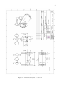
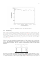
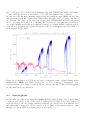
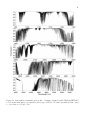
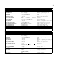
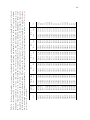
1
EUROPEAN SOUTHERN OBSERVATORY
Organisation Européene pour des Recherches Astronomiques dans l’Hémisphère Austral
Europäische Organisation für astronomische Forschung in der südlichen Hemisphäre
ESO - European Southern Observatory
Karl-Schwarzschild Str. 2, D-85748 Garching bei München
Very Large Telescope
Paranal Science Operations
CRIRES User Manual
Doc. No. VLT-MAN-ESO-14500-3486
Issue 87.3, Date 25/12/2010
R. Siebenmorgen, A. Smette, J.Smoker 25/12/2010
Prepared
. . . . . . . . . . . . . . . . . . . . . . . . . . . . . . . . . . . . . . . . . .
Date
Approved
A. Smette
. . . . . . . . . . . . . . . . . . . . . . . . . . . . . . . . . . . . . . . . . .
Date
Released
Signature
Signature
C. Dumas
. . . . . . . . . . . . . . . . . . . . . . . . . . . . . . . . . . . . . . . . . .
Date
Signature
CRIRES User Manual
VLT-MAN-ESO-14500-3486
This page was intentionally left blank
ii
CRIRES User Manual
VLT-MAN-ESO-14500-3486
iii
Change Record
Issue/Rev.
79.1
79.2
79.3
79.4
80.1
Date
29/08/06
08/09/06
20/12/06
21/12/06
05/03/07
Section/Parag. Reason/Initiation/Documents/Remarks
affected
all
all
all
14,15
0,1
3
6
5
8
80.2
80.3
80.4
80.5
10
11
12
12/03/07 0,8.1,10.3
7.2,14.2
20/03/07
26/03/07
07/05/07
21/05/07
05/06/07
09/06/07
09/06/07
09/06/07
19/06/07
19/06/07
20/06/07
20/06/07
20/06/07
20/06/07
15
15
1
14.2
7.2
0,1,7.4
14.1.1
12
1.4,6.4
8.4
17,18
11.1,14.1
9.3
14.2
RSI,ASM: First release, issued for P79 Phase1
ASM: Sec. 11, corrected wavelength table
RSI, ASM, comments DMD
ASM, minor editorial corrections
ASM, corrected layout figure and description
added a web-link
corrected detector gain
added comments on a non-linearity correction method
minor updates and corrected typos
updated limiting mag. in noAO
added subsection on entrance window transmission
updated sensitivities
updated overheads
added 3 recommended DIT values, updated text
updated
corrected typos
added paragraph on gas-cell
and generic offsets template
corrected J band wavelength ranges
corrected missing entries in Table 4
corrected description
new observation template
added link to N2O line list; 1st results on RV accuracy
corrected slit length and slit viewer f-o-v
corrected typo in RA offset
daytime wavecal only for λ < 2400 nm
contact information, odd-even
add important note on intermediate slit
new section 17, update §18
added comments on ext. objects, moving targets
added comments on std stars
added gas cell P2PP parameter description
CRIRES User Manual
81.1 31/08/07
31/08/07
31/08/07
31/08/07
01/09/07
01/09/07
01/09/07
01/09/07
01/09/07
02/09/07
02/09/07
81.2 19/11/07
20/11/07
21/11/07
21/11/07
22/11/07
18/12/07
18/12/07
27/12/07
27/12/07
27/12/07
27/12/07
27/12/07
27/12/07
28/12/07
82.1 20/01/08
20/01/08
03/03/08
03/03/08
03/03/08
03/03/08
03/03/08
03/03/08
82.2 19/06/08
19/06/08
19/06/08
23/06/08
23/06/08
23/06/08
23/06/08
25/06/08
25/06/08
25/06/08
25/06/08
VLT-MAN-ESO-14500-3486
8.4
8.2
10.3
15
6.4
9.1
11.2.1
8.2
11.4
5, 7.5
11.5
11.2.4, 14.2, 14.2.5
14.1.3
1.5
10.1
14.2.4
Table 1
7.2
Tables 4a-5h
§7.5, 8.4,9.1, 9.2.1
§9.2.3, 10.2, 11.1, 11.2.1
§11.2.4,10.1,13.1, 14.1, 5
§11.5.3, 5.1
§7.3, 5.2
§5.1.2
§7.2
§20
§7.1
§8.4
§11.7
§11.6
§14.1.7
§18
§10.2
Table 3
§9.1,Fig.25
§7.2
§14.1.2 14.3.6
§1.5
§2.1, 11.2.5
§12
§14.1.7
§7.1
§11.4
iv
updated
Added Fig. 22: comparison UVES vs CRIRES
Table 3 (overheads) updated
Slightly changed captions
Added links to method and reference frames
Added link to ETC
Added para.: choice of a SVGS in crowded field
Added para. on slit loss due to diff. refraction
Added requirement for fc
Figures added (AO performance, resolving power)
Add a para. on airmass
Added SpectroAstrometry template
Change default value of SEQ.NGS.USELASTSKY to T
New section: NEWS
Added: specific comments for SM (telluric OBs)
Expanded description of generic offsets template
Dark current values corrected
Changed comment regarding gas-cells
Wavelength settings updated
typos corrected
typos corrected
typos corrected
clarified
updated
AO star bright mag. limit updated
updated available gas-cells
added section
updated: new configuration table
updated
numbering changed
new sub-section on water vapor
updated
updated
ETC updated: precipitable water vapor
incl. overhead for derotator motion in spectroastrometry
added a fig. with water vapor only transmission
ThAr fibers, CO gas-cell and visitor gas-cells
Updated for the use of CO gas-cell
Updated
Updated for ThAr fiber
calibration plan updated
added note regarding slit width
Added note: vacuum wavelength are used
Added note regarding multiple stars
CRIRES User Manual
83.1 29/08/08
29/08/08
29/08/08
29/08/08
29/08/08
83.2 19/12/08
19/12/08
19/12/08
19/12/08
19/12/08
19/12/08
84.1 04/03/09
04/03/09
04/03/09
04/03/09
04/03/09
04/03/09
04/03/09
84.2 29/05/09
30/05/09
30/05/09
30/05/09
30/05/09
15/06/09
Tab. 8a
§1.5
§20.1
§7.2.1
§7.4
§7.2.2
§7.5
§6.5
§14.1.3
§8.2
§1.3,11, 20.2
§1.5
§14.1
§7.1
§7.2.2
§11.3
Tab. 3
§11.1
§1.5
§5.1.3
§5.1
§7.2.1
§7.4, Fig 18
§14
VLT-MAN-ESO-14500-3486
v
updated with CO gas-cell for order 24
news updated
checklist updated
update on identification of ThAr lines
added not regarding slit width
radial-velocity measurements: added
spectral resolution: updated
linearity: added
WFS last sky measurements: updated
limitations due to differential refraction: removed
P2PP links: updated
Section updated
Note added
Slit wider than 0.400 should be avoided.
Note added regarding radial velocity measurements
New readout mode
Overheads table updated
Differential tracking
Section updated
Note added
Max. distance AO star - science target corrected
Updated with new ThAr atlas information
F-o-v updated following the May09 intervention
Added description of differential tracking
Added description of readout modes
17/06/09 §6, 11.3
Updated to take into account the new readout mode
17/06/09 §7.1
Updated to take into account the new configuration table
17/06/09 Tab 4a -7
Updated to take into account the new configuration table
17/06/09 §19
Differential tracking section added
17/06/09 §10.4
Differential chromatic effect section added
18/06/09 Tab 3
Overheads updated
01/07/09 §7.5
Section updated
01/07/09 §11.5
Section updated
85.1 31/08/09 §11.3 and 14.1.8 DIT setting: §reworded
31/08/09 §14.2
updated
31/08/09 §19.3
note added
31/08/09 §7.2.1
gas-cell: note added
31/08/09 §1.5
updated
85.2 31/08/09 §1.5
updated
25/12/09 §6.2
comment on detector glow
25/12/09 §7.2.2
updated with new RV refs
25/12/09 §7.5
resolving power reproducability section ammended
25/12/09 §8.2
UVES/CRIRES comparison updated
25/12/09 §11.3 and 14.1.8 DIT setting:§further updated
25/12/09 §14.3.2
FF parameters; updated advice for extended targets
25/12/09 §14.3.3
updated wavelength calibration section
25/12/09 §14.3.4
updated dark parameters
25/12/09 Table 15.1
tables of reference wavelengths updated with new
encoder values.
25/12/09 Figure 18
slit and science detector geometry figure changed
25/12/09 §19.3
updated differential tracking section
CRIRES User Manual
VLT-MAN-ESO-14500-3486
vi
86.1 26/02/10
26/02/10
s6/02/10
26/02/10
26/02/10
26/02/10
26/02/10
26/02/10
26/02/10
86.2 24/06/10
Minor updates for P86 phase I
§1.5
updated news
§2.1
updated optics section
§7.1
updated wavelength settings section
§8.4
updated reproducability section
§7.2.2
updated with new RV refs
§7.5
updated spectral resolving power section
§8.2
note added about overheads
§10.1
note added about OBs over 1 hour needing waiver
§1.3
note added about order contamination for wide slits,
slit width variation and AO-related issues to be aware of
24/06/10 §1.5
news section updated to point at news webpage
24/06/10 §7.2.2
updated RV ref
24/06/10 §10.5
Notes for visiting astronomers updated
87.1 24/08/10 §1.3
Note that the entrance slit will likely be replaced
in future
24/08/10 §2.2
Temperature of detectors 27 K
24/08/10 §5.1.2
Typos
24/08/10 §7.5
Emphasise that slit width of <0.2” not possible.
24/08/10 §9.4
Comment about backup targets incse of high winds added
24/08/10 §10.2
Link added for Paranal PWV measuremants
24/08/10 §10.5
Figure showing order contamination added
24/08/10 §11.5.4 No AO in THK cloud for R<10.5 mag
24/08/10 §11.6
PWV measurement url added
24/08/10 §14.1.7 Typos
87.2 16/09/10 Fig. 18 Geometry of SV camera changed after Sept 2010
intervention
87.3 25/12/10 §1.5
News updated
25/12/10 §7.1
Metrology not yet implemented
25/12/10 §7.2.1
Typos
25/12/10 §7.2.2
Typos
25/12/10 §7.2.4
AO/NoAO is possible without gas cells in the beam
25/12/10 §7.3
Atlas of CRIRES flatfields reference
25/12/10 §10.2
ETC values given per pixel
25/12/10 §10.3
Overheads section reworded
25/12/10 §11.1
Typos
25/12/10 §11.3
Slit width can be changed independently of the DIT
25/12/10 §11.2.1 Waiver needed in SM for slit wider than 0.4 arcseconds
25/12/10 §14.1.7 Waiver needed in SM for slit wider than 0.4 arcseconds
25/12/10 §14.2.3 Only one λ setting if win=64 pixels for FowlerNsampGrstWin
25/12/10 §20.2
Phase 2 guidlines section expanded
First version of the manual was written by R.Siebenmorgen and A.Smette. L. Tacconi-Garman
and M. Hilker provided numerous comments on the various versions of this manual that greatly
improved its accuracy and clarity. The content of §7.2.2 (RV measurements) was originally
based on discussions with H.-U. Kaeufl, P. Figueroa and Andreas Seifarht.
CRIRES User Manual
VLT-MAN-ESO-14500-3486
Abbreviations and Acronyms
AO
APD
BOB
CPL
CRIRES
DM
DMO
ESO
ETC
FC
FoV
FWHM
NGS
NIR
NIST
OB
P2PP
PSF
QC
RTC
RTD
SDD
SM
SNR
SR
TIO
TTM
USD
VLT
VM
WF
WFS
Adaptive optics
Avalanche photo-diode
Broker of observation blocks
Common Pipeline Library
Cryogenic high-resolution infrared echelle spectrograph
Deformable mirror
Data management and operations division
European Southern Observatory
Exposure time calculator
Finding chart
Field of view
Full width at half maximum
Natural guide stars
Near infrared
National Institute of Standards and Technology
Observation block
Phase II proposal preparation
Point spread function
Quality control
Real time computer
Real time display
Software Development Division
Service mode
Signal-to-noise ratio
Strehl ratio
Telescope and instrument operator
Tip-tilt mount
User support department
Very large telescope
Visitor mode
Wave front
Wave front sensor
vii
CRIRES User Manual
VLT-MAN-ESO-14500-3486
Overview
Calibration system
Adaptive optics
Slit length
Slit width
Echelle grating
Resolving power
Wavelength range
Free spectral range
Detector science array
Pixel scale
Slit viewer: filters
Slit viewer: detector
Slit viewer: field-of-view
Slit viewer: pixel scale
Pre-disperser
halogen lamp, IR-emitter, ThAr, N2 O, CO, visitor gas cells
60-actuator curvature sensing MACAO system
≈ 40 00
0.05 00 – 3.0 00 : recommended 0.2 00 – 0.4 00
40 × 20cm, 31.6 lines/mm, 63.5o blaze angle
100, 000 (0.2 00 ); 50, 000 (0.4 00 slit)
0.95µm ≤ λ ≤ 5.2µm
from λ/70 at 1µm to λ/50 at 5µm
4096 × 512 pixels using 4 Aladdin III detectors
0.086 00
J, H, K, 2 H + neutral density
Aladdin III array
≈ 35 00 × 43 00
≈ 0.047 00
ZnSe prism
viii
CRIRES User Manual
VLT-MAN-ESO-14500-3486
This page was intentionally left (almost) blank
ix
CRIRES User Manual
VLT-MAN-ESO-14500-3486
x
Contents
1 Introduction
1.1 Science drivers . . . . . . . . . . . . . .
1.2 Structure and scope of the User Manual
1.3 More important information on CRIRES
1.4 Contact Information . . . . . . . . . . .
1.5 News . . . . . . . . . . . . . . . . . . . .
I
.
.
.
.
.
.
.
.
.
.
.
.
.
.
.
.
.
.
.
.
.
.
.
.
.
.
.
.
.
.
.
.
.
.
.
.
.
.
.
.
.
.
.
.
.
.
.
.
.
.
.
.
.
.
.
.
.
.
.
.
.
.
.
.
.
.
.
.
.
.
.
.
.
.
.
.
.
.
.
.
.
.
.
.
.
.
.
.
.
.
.
.
.
.
.
.
.
.
.
.
.
.
.
.
.
The instrument
1
1
2
3
4
4
8
2 Cold part: the spectrometer
2.1 Optics . . . . . . . . . . . . . . . . . . . . . . . . . . . . . . . . . . . . . . . .
2.2 Mechanics . . . . . . . . . . . . . . . . . . . . . . . . . . . . . . . . . . . . . .
2.3 Detectors . . . . . . . . . . . . . . . . . . . . . . . . . . . . . . . . . . . . . .
8
9
9
10
3 Warm part: the adaptive optics system
3.1 Introduction . . . . . . . . . . . . . . .
3.1.1 Atmospheric turbulence . . . . .
3.1.2 Adaptive Optics . . . . . . . . . .
3.2 Hardware description . . . . . . . . . . .
3.2.1 The corrective optics . . . . . . .
3.2.2 The Wavefront Sensor . . . . . .
3.2.3 Control loop . . . . . . . . . . . .
3.2.4 Membrane setting . . . . . . . . .
11
11
11
12
13
13
13
15
17
II
.
.
.
.
.
.
.
.
.
.
.
.
.
.
.
.
.
.
.
.
.
.
.
.
.
.
.
.
.
.
.
.
.
.
.
.
.
.
.
.
.
.
.
.
.
.
.
.
.
.
.
.
.
.
.
.
.
.
.
.
.
.
.
.
.
.
.
.
.
.
.
.
.
.
.
.
.
.
.
.
.
.
.
.
.
.
.
.
.
.
.
.
.
.
.
.
.
.
.
.
.
.
.
.
.
.
.
.
.
.
.
.
.
.
.
.
.
.
.
.
.
.
.
.
.
.
.
.
.
.
.
.
.
.
.
.
.
.
.
.
.
.
.
.
.
.
.
.
.
.
.
.
.
.
.
.
.
.
.
.
.
.
.
.
.
.
.
.
Instrument Performance
18
4 Overview
18
5 AO performance
5.1 AO guide stars . . . . . . . . . . . .
5.1.1 The distance of the AO star .
5.1.2 The brightness of the AO star
5.1.3 The color of the AO star . . .
5.2 Limiting magnitude of slit viewer . .
.
.
.
.
.
19
19
20
20
21
21
6 Detector characteristics
6.1 Dark and gain . . . . . . . . . . . . . . . . . . . . . . . . . . . . . . . . . . . .
6.2 Glow . . . . . . . . . . . . . . . . . . . . . . . . . . . . . . . . . . . . . . . .
6.3 Fringes . . . . . . . . . . . . . . . . . . . . . . . . . . . . . . . . . . . . . . . .
22
23
23
23
.
.
.
.
.
.
.
.
.
.
.
.
.
.
.
.
.
.
.
.
.
.
.
.
.
.
.
.
.
.
.
.
.
.
.
.
.
.
.
.
.
.
.
.
.
.
.
.
.
.
.
.
.
.
.
.
.
.
.
.
.
.
.
.
.
.
.
.
.
.
.
.
.
.
.
.
.
.
.
.
.
.
.
.
.
.
.
.
.
.
.
.
.
.
.
.
.
.
.
.
.
.
.
.
.
.
.
.
.
.
CRIRES User Manual
VLT-MAN-ESO-14500-3486
xi
6.4 Odd-even effect . . . . . . . . . . . . . . . . . . . . . . . . . . . . . . . . . . .
6.5 Correcting for detector non-linearity . . . . . . . . . . . . . . . . . . . . . . .
7 Characteristics of the spectrograph
7.1 Wavelength settings . . . . . . . . . . . . . . . .
7.2 Wavelength calibration . . . . . . . . . . . . . .
7.2.1 Standard means: ThAr lamp and N2 O and
7.2.2 Radial velocity measurements . . . . . . .
7.2.3 Visitor gas-cells . . . . . . . . . . . . . . .
7.2.4 Observations without gas cells . . . . . . .
7.3 Flat fields . . . . . . . . . . . . . . . . . . . . . .
7.4 Spectrograph field-of-view, slit width and seeing .
7.5 Spectral resolving power . . . . . . . . . . . . . .
8 System efficiency and throughput
8.1 Transmission of the entrance window
8.2 Sensitivity . . . . . . . . . . . . . . .
8.3 Optical ghosts . . . . . . . . . . . . .
8.4 Stability and reproducibility . . . . .
III
.
.
.
.
.
.
.
.
.
.
.
.
.
.
.
.
.
.
.
.
.
.
.
.
.
.
.
.
. . . . . . . .
. . . . . . . .
CO gas-cells
. . . . . . . .
. . . . . . . .
. . . . . . . .
. . . . . . . .
. . . . . . . .
. . . . . . . .
.
.
.
.
.
.
.
.
.
.
.
.
.
.
.
.
.
.
.
.
.
.
.
.
.
.
.
.
.
.
.
.
.
.
.
.
.
.
.
.
.
.
.
.
.
.
.
.
.
.
.
.
.
.
.
.
.
.
.
.
.
.
.
.
.
.
.
.
.
.
.
.
.
.
.
.
.
.
.
.
.
.
.
.
.
.
.
.
.
.
.
.
.
.
.
.
.
.
.
.
.
.
.
.
.
.
.
.
.
.
.
.
.
.
.
.
.
.
.
.
.
.
.
24
24
.
.
.
.
.
.
.
.
.
26
26
26
26
28
30
31
31
32
35
.
.
.
.
36
36
37
38
39
Observing with CRIRES at the VLT
40
9 Introduction
9.1 Atmospheric transmission . . . . . . . . . . . . . . . .
9.2 Background removal . . . . . . . . . . . . . . . . . . .
9.2.1 Sky emission spectrum . . . . . . . . . . . . . .
9.2.2 Nodding . . . . . . . . . . . . . . . . . . . . . .
9.2.3 Jittering . . . . . . . . . . . . . . . . . . . . . .
9.3 Flux calibration and telluric correction . . . . . . . . .
9.3.1 General procedure . . . . . . . . . . . . . . . .
9.3.2 Telluric correction . . . . . . . . . . . . . . . . .
9.3.3 Hot stars as telluric standards . . . . . . . . . .
9.3.4 Late–type stars or G stars as telluric standards
9.3.5 Catalogs . . . . . . . . . . . . . . . . . . . . . .
9.4 The influence of the Moon . . . . . . . . . . . . . . . .
.
.
.
.
.
.
.
.
.
.
.
.
40
40
40
40
40
40
43
43
43
43
44
44
44
.
.
.
.
.
45
45
45
47
47
48
10 Observing in Visitor and Service
10.1 Overview . . . . . . . . . . . . .
10.2 The Exposure Time Calculator
10.3 Overheads . . . . . . . . . . .
10.4 Differential effects . . . . . . . .
10.5 Visitor Mode observations . . .
Mode
. . . .
. . . .
. . . .
. . . .
. . . .
.
.
.
.
.
.
.
.
.
.
.
.
.
.
.
.
.
.
.
.
.
.
.
.
.
.
.
.
.
.
.
.
.
.
.
.
.
.
.
.
.
.
.
.
.
.
.
.
.
.
.
.
.
.
.
.
.
.
.
.
.
.
.
.
.
.
.
.
.
.
.
.
.
.
.
.
.
.
.
.
.
.
.
.
.
.
.
.
.
.
.
.
.
.
.
.
.
.
.
.
.
.
.
.
.
.
.
.
.
.
.
.
.
.
.
.
.
.
.
.
.
.
.
.
.
.
.
.
.
.
.
.
.
.
.
.
.
.
.
.
.
.
.
.
.
.
.
.
.
.
.
.
.
.
.
.
.
.
.
.
.
.
.
.
.
.
.
.
.
.
.
.
.
.
.
.
.
.
.
.
.
.
.
.
.
.
.
.
.
.
.
.
.
.
.
.
.
.
.
.
.
.
.
.
.
.
.
.
.
.
.
.
.
.
.
.
.
.
.
.
.
.
.
.
.
.
.
.
.
.
.
.
.
.
.
.
.
.
.
.
.
.
.
.
.
.
.
.
.
CRIRES User Manual
VLT-MAN-ESO-14500-3486
xii
11 Preparation of Observation Blocks
11.1 Information required . . . . . . . . . . . . . . . . . . . . . . . .
11.2 Observation Blocks and Templates . . . . . . . . . . . . . . . .
11.2.1 Acquisition . . . . . . . . . . . . . . . . . . . . . . . . .
11.2.2 Acquisition sequences with AO . . . . . . . . . . . . . .
11.2.3 Acquisition sequences without AO . . . . . . . . . . . . .
11.2.4 Science . . . . . . . . . . . . . . . . . . . . . . . . . . . .
11.2.5 Calibration . . . . . . . . . . . . . . . . . . . . . . . . .
11.3 Detector read-out mode and DIT setting . . . . . . . . . . . . .
11.4 README and finding charts . . . . . . . . . . . . . . . . . . .
11.5 Constraints . . . . . . . . . . . . . . . . . . . . . . . . . . . . .
11.5.1 Moon . . . . . . . . . . . . . . . . . . . . . . . . . . . .
11.5.2 Seeing and Strehl ratio for adaptive optics observations .
11.5.3 Seeing for seeing limited observations, no adaptive optics
11.5.4 Transparency . . . . . . . . . . . . . . . . . . . . . . . .
11.5.5 Airmass . . . . . . . . . . . . . . . . . . . . . . . . . . .
11.6 Water vapor . . . . . . . . . . . . . . . . . . . . . . . . . . . . .
11.7 Offset conventions and definitions . . . . . . . . . . . . . . . . .
IV
.
.
.
.
.
.
.
.
.
.
.
.
.
.
.
.
.
.
.
.
.
.
.
.
.
.
.
.
.
.
.
.
.
.
.
.
.
.
.
.
.
.
.
.
.
.
.
.
.
.
.
.
.
.
.
.
.
.
.
.
.
.
.
.
.
.
.
.
.
.
.
.
.
.
.
.
.
.
.
.
.
.
.
.
.
.
.
.
.
.
.
.
.
.
.
.
.
.
.
.
.
.
.
.
.
.
.
.
.
.
.
.
.
.
.
.
.
.
.
.
.
.
.
.
.
.
.
.
.
.
.
.
.
.
.
.
51
51
52
52
53
55
55
55
56
57
58
58
58
59
59
59
59
59
Reference material
61
12 CRIRES calibration plan
61
13 Data format and reduction
13.1 Format . . . . . . . . . . . . . . . . . . . . . . . . . . . . . . . . . . . . . . . .
13.2 Pipeline . . . . . . . . . . . . . . . . . . . . . . . . . . . . . . . . . . . . . . .
62
62
62
14 Template parameters
14.1 Acquisition templates . . . . . . . . . . . . .
14.1.1 Target and SVGS parameters . . . .
14.1.2 Gas cell . . . . . . . . . . . . . . . .
14.1.3 NGS parameters . . . . . . . . . . .
14.1.4 Parameters related to the slit viewer
14.1.5 Telescope guide star parameters . . .
14.1.6 Derotator parameters . . . . . . . . .
14.1.7 Spectrograph parameters . . . . . . .
14.1.8 Science detector parameters . . . . .
14.1.9 Notes . . . . . . . . . . . . . . . . .
14.2 Observation templates . . . . . . . . . . . .
14.2.1 Detector . . . . . . . . . . . . . . . .
14.2.2 Gas cell . . . . . . . . . . . . . . . .
63
63
63
65
65
66
66
67
67
68
68
68
69
69
.
.
.
.
.
.
.
.
.
.
.
.
.
.
.
.
.
.
.
.
.
.
.
.
.
.
.
.
.
.
.
.
.
.
.
.
.
.
.
.
.
.
.
.
.
.
.
.
.
.
.
.
.
.
.
.
.
.
.
.
.
.
.
.
.
.
.
.
.
.
.
.
.
.
.
.
.
.
.
.
.
.
.
.
.
.
.
.
.
.
.
.
.
.
.
.
.
.
.
.
.
.
.
.
.
.
.
.
.
.
.
.
.
.
.
.
.
.
.
.
.
.
.
.
.
.
.
.
.
.
.
.
.
.
.
.
.
.
.
.
.
.
.
.
.
.
.
.
.
.
.
.
.
.
.
.
.
.
.
.
.
.
.
.
.
.
.
.
.
.
.
.
.
.
.
.
.
.
.
.
.
.
.
.
.
.
.
.
.
.
.
.
.
.
.
.
.
.
.
.
.
.
.
.
.
.
.
.
.
.
.
.
.
.
.
.
.
.
.
.
.
.
.
.
.
.
.
.
.
.
.
.
.
.
.
.
.
.
.
.
.
.
.
.
.
.
.
CRIRES User Manual
VLT-MAN-ESO-14500-3486
xiii
14.2.3 CRIRES spec obs AutoNodOnSlit and CRIRES spec obs SpectroAstrometry:
nodding and jittering . . . . . . . . . . . . . . . . . . . . . . . . . . . . 69
14.2.4 CRIRES spec obs GenericOffset only: list of offsets . . . . . . . . . . . 70
14.2.5 CRIRES spec obs SpectroAstrometry only: list of derotator angles, jitter reset . . . . . . . . . . . . . . . . . . . . . . . . . . . . . . . . . . . 72
14.3 Calibration templates . . . . . . . . . . . . . . . . . . . . . . . . . . . . . . . . 73
14.3.1 Standard star or telluric observations . . . . . . . . . . . . . . . . . . . 73
14.3.2 Flat field . . . . . . . . . . . . . . . . . . . . . . . . . . . . . . . . . . 73
14.3.3 Wavelength calibration . . . . . . . . . . . . . . . . . . . . . . . . . . . 74
14.3.4 Darks . . . . . . . . . . . . . . . . . . . . . . . . . . . . . . . . . . . . 74
14.3.5 Sky observation . . . . . . . . . . . . . . . . . . . . . . . . . . . . . . . 75
14.3.6 Template signatures . . . . . . . . . . . . . . . . . . . . . . . . . . . . 76
15 CRIRES standard wavelength settings
15.1 Wavelength ranges . . . . . . . . . . . . . . . . . . . . . . . . . . . . . . . . .
15.2 Wavenumber ranges . . . . . . . . . . . . . . . . . . . . . . . . . . . . . . . . .
83
83
95
16 Free wavelength settings
107
17 Reference wavelengths common to different orders
109
18 Calibration source for wavelength calibration
110
19 Differential tracking
113
19.1 Introduction . . . . . . . . . . . . . . . . . . . . . . . . . . . . . . . . . . . . . 113
19.2 Tracking tables . . . . . . . . . . . . . . . . . . . . . . . . . . . . . . . . . . . 113
19.3 Acquisition and observation . . . . . . . . . . . . . . . . . . . . . . . . . . . . 115
V
Tips for successful observations
116
20 Checklist
116
20.1 Phase 1 . . . . . . . . . . . . . . . . . . . . . . . . . . . . . . . . . . . . . . . 116
20.2 Phase 2 . . . . . . . . . . . . . . . . . . . . . . . . . . . . . . . . . . . . . . . 117
CRIRES User Manual
1
VLT-MAN-ESO-14500-3486
1
Introduction
The cryogenic high-resolution IR echelle spectrograph – CRIRES – is the infrared (0.95µm
– 5.2µm) high–resolution spectrograph located at the Nasmyth A focus of UT1 (Antu). It
provides long–slit (∼40 00 ) spectroscopy with a spatial sampling of 0.086 00 . Spatial resolution
and signal–to–noise ratio can be maximized by the optional use of a MACAO adaptive optics
system equipped with an optical (R band) wavefront sensor.
The main optical elements consist of a prism acting as a pre–disperser and a 31.6 lines/mm
echelle grating. Total spectral coverage per individual wavelength setting is ∼ λ/70 thanks to
an array of four Aladdin III detectors. Acquisition and guiding are performed by means of a
slit viewer equipped with an additional Aladdin III detector and a series of 5 filters (J,H,K
and two neutral density H filters).
CRIRES has been designed to exploit the enormously enhanced sensitivity provided by a
spectroscopic instrument with a large detector array at an 8m telescope. The quantitative and
qualitative improvements of observational capabilities affect all scientific applications aiming
at fainter objects with higher spatial (extended sources), spectral and temporal resolutions.
Indeed, CRIRES provides:
• High-resolution spectroscopy in the 1-5 µm range at the VLT. This instrument employs
the largest available grating for a spectral resolving power of up to ≈100,000 (for 2 pixel
Nyquist sampling) with a 0.200 slit;
• Spectral coverage maximized through four 1024 x 512 pixel InSb detector arrays in the
focal plane;
• Spectral imaging using a 4000 long slit;
• Adaptive Optics to maximize the signal-to-noise ratio (SNR) and spatial resolution.
Functionally, the instrument can be divided into four units:
1. The fore-optics unit provides field de-rotation, cold pupil and field stops, curvature
sensing adaptive optics, and slit viewing.
2. The prism pre-disperser isolates one echelle order and minimizes the total amount of
background entering the high-resolution unit.
3. The high-resolution unit comprises the collimator, the echelle which is tilt-tuned for
wavelength selection, the camera and the science detectors.
4. The calibration unit outside the cryogenic environment contains the light sources for
wavelength calibration and detector flat-fielding.
1.1
Science drivers
Thanks to CRIRES, new phenomena and objects are now available for spectroscopic studies.
Some highlights are:
• Extra-solar planets:
CRIRES User Manual
VLT-MAN-ESO-14500-3486
2
– radial velocities
– spectroscopy of CO, CH4
• Solar system:
– Giant planets, Titan: H+
3 , CH4 , CH3 , NH3 , HCN, ...
– Terrestrial planets: CO, HCL, HDO, H2 O, ...
– Mars: imaging spectroscopy of CO depletion at 40km resolution
– Io: volcanic activity (SO2 )
– Pluto, Charon, Triton: CO, CH4 search
– Comets: H2 O abundance, temperatures, velocities
• Stars:
– stellar evolution and nucleosynthesis: CNO abundance
– stellar mass
– stellar radii
– stellar winds and mass loss
– atmospheric structure and oscillations
– magnetic field structure
• Star formation and ISM:
– accretion and outflows
– ISM chemistry and cloud structures: H+
3 , H2 O, CH4 , ...
• Extragalactic astronomy:
– AGN: velocity structure of the broad and narrow line region, [FeII], H2 lines in low
extinction regions, H recombination
– fine structure lines
1.2
Structure and scope of the User Manual
The CRIRES user manual is structured as follows:
• Part I provides a technical description of CRIRES and its adaptive optics system (AO).
• Part II details the instrument performance.
• Part III describes the commonly used observing techniques in the infrared, summarizes
the CRIRES observing modes and provides guidelines for Phase 2 preparation.
• Reference material is given in Part IV. It includes a description of the calibration plan,
the data format, the template reference guide and the defined wavelength settings.
• Finally, Part V provides a number of recommendations written to increase the chances
that a program is executed successfully.
CRIRES User Manual
1.3
VLT-MAN-ESO-14500-3486
3
More important information on CRIRES
CRIRES is a complicated instrument. A handful of the things that you must remember are:
• Entrance slit widths of more than 0.4 arcseconds lead to contamination of your spectra
by adjacent orders so are in general not recommended.
• AO observations of bright targets with thick cloud are not allowed due to the possibility
of damaging the Avalanche Photo Diodes.
• The AO star has to be fainter than R∼0.2, depending on its colour.
• When planning AO observations, make sure that the sky position for the field selector
is blank.
• The CRIRES entrance slit shows variations in its width exceeding 30 per cent although
efforts are made to reduce this to around 10 per cent with some overhead. In the future
it is likely that the slit mechanism will be replaced, perhaps to fixed slits.
All CRIRES related manuals are available on the CRIRES instrument web pages together
with the most updated information on the instrument:
http://www.eso.org/instruments/crires/
Both Service and Visitor mode Observation Blocks (OBs) should be prepared with the latest
version of the Phase 2 Proposal Preparation tool (P2PP), available at:
http://www.eso.org/sci/observing/phase2/P2PP/P2PPTool.html.
Information for the preparation of Service mode observations with CRIRES are available at:
http://www.eso.org/sci/observing/phase2/SMGuidelines.html#CRIRES
Visiting astronomers do not need to submit Observation Blocks in advance of their observations. However, they should prepare them before arriving at the observatory or, at the latest,
at the observatory the nights before their observing run. They will find further instructions
on the Paranal Science Operations web page and the Paranal Observatory home page:
http://www.eso.org/paranal/
http://www.eso.org/paranal/sciops/
In particular, visiting astronomers should read the following webpage:
http://www.eso.org/sci/facilities/paranal/instruments/crires/visitor.html
Reference frames, static calibration frames, information regarding the CRIRES pipeline and
quality control can be found at:
http://www.eso.org/observing/dfo/quality/
http://www.eso.org/observing/dfo/quality/index_crires.html
CRIRES User Manual
1.4
VLT-MAN-ESO-14500-3486
4
Contact Information
In case of specific questions related to Service Mode observations and proposal preparation
please contact the ESO User Support Department:
usd–[email protected]
For Visitor Mode observations please contact the Paranal Science Operations Team. For
general information, use
[email protected]
For specific questions regarding the use of CRIRES, use:
[email protected]
1.5
News
Recall that the most up-to-date information on CRIRES is found on the webpage http:
//www.eso.org/sci/facilities/paranal/instruments/crires/news.html
Since the release of User Manual v86.2
• Further interventions on CRIRES (during May, July, August, September and November)
in order to correct problems with misalignment of the intermediate and entrance slit and
the removal and re-integration of the warm part of the instrument due M1/M3 recoating
and maintenance.
Since the release of User Manual v86.1
• An intervention on CRIRES was performed to fix problems with the cooling during May
2010 that meant the instrument was offline for four weeks.
Since the release of User Manual v85.2
• Metrology fibres should be in operation in time for P86. Users are reminded that these
fibres will only be available in standard and not free settings.
• After every change of entrance slit width the width is now measured to try and ensure
that it is within 10 percent of the requested value.
Since the release of User Manual v85.1
• The CRIRES spec cal LampFlats template now accepts new parameters: it allows to
set the maximum flux over the frame, as well as the entrance slit width.
• An intervention took place in December 2009 to finalize the installation of metrology
fibers. This systems aims at providing repeatability of the wavelength zero point and
dispersion to guarantee reproducibility to 1/10 pixel, for the standard settings. Associated overheads have already been included in Table 3. The CRIRES news pages will
be updated with the results of the intervention with the results of reproducibility tests.
The positioning of the lines on the detector have shifted by ∼30 pixels in some settings.
Tables 15.1, 6a and 6b have been updated.
CRIRES User Manual
VLT-MAN-ESO-14500-3486
5
Since the release of User Manual v84.2
• The entrance slit is now the least reproducible part of the instrument with variations of
up to 50% in slit width. Technical tests will take place on September 3 and 4 to check
the entrance slit width with the aim of insuring a reproducibility at the 10% level.
• Differential tracking has been offered in service mode since P85.
Since the release of User Manual v84.1
• An intervention took place in May 2009:
– the science mosaic was moved so that its center its closer to the optical axis of the
instrument; an internal baffle was modified; as a consequence, the field-of-view of
the science detector is ≈ 40”; Fig. 18 has been updated;
– metrology fibers have been installed which will guarantee a better wavelength setting reproducibility for data taken after an intervention foreseen in December 2009.
Until then, the only consequence for the user is the presence of additional spectra
on ThAr exposures; an example is given in Fig. 15;
– the intermediate slit mechanism has been replaced by a more reliable one; it improves the wavelength setting reproducibility and decreases the uncertainty on the
wavelength range affected by contamination by adjacent orders. As a consequence,
the configuration table and standard settings had to be revised (see Tables 4a - 4k
and Tables 5a - 5k) allowing a complete coverage without contamination by adjacent
orders. Overhead for change of wavelength setting has significantly decreased;
– the thermal control of the instrument has been further improved;
• The pipeline has been modified such that it is able to process data with different illumination areas: it automatically recognizes which area is illuminated depending on the date
the data were taken. In particular, it recognizes data obtained between January 2009
and May 2009, and after May 2009. Cf. http://www.eso.org/sci/data-processing/
software/pipelines/index.html.
• the ThAr catalogue has been updated with newly identified lines, see §7.2.
Since the release of User Manual v83.2
• An intervention took place in January 2009. Its main objective was to install new cryocoolers. Indeed, the previous ones were causing a lot of vibrations strongly degrading the
quality of the VLTI observations: consequently, CRIRES cryo-coolers had to be stopped
during VLTI UT runs after which a further ∼ 3−4 days were lost for CRIRES operations
while the instrument reached its operating temperature. The problems affecting the
quality of the encoder reading for the grating, prism and entrance and intermediate slits
have been solved considerably improving the repeatability of the functions. Quantitative
values on this respect will be made available for the v84.2 of this manual.
• Considerable work has been completed to improve the maintainability of the observation
and instrument control software. For the user, its main visible part is the full implementation of the compensation for the differential refraction, as well as the implementation
of the differential tracking mode.
CRIRES User Manual
VLT-MAN-ESO-14500-3486
6
• An additional intervention will take place in May 2009. Its main goal is to implement a
metrology system to allow to configure the spectrograph in a very accurate and reproducible way.
• A new readout mode has been implemented to window the detector 2 and 3. In turn, it
allows to use DITs as short as 0.15s.
Since the release of User Manual v83.1 The announced major change to the instrument
control and observing software was successfully implemented in November 2008, although still
incomplete at the time of issuing this manual. The missing parts will be implemented in
February and March 2009.
Since the release of User Manual v82.2 :
• the CRIRES spec cal Wave template was modified to make use of a variable neutral
density filter : this allows optimal illumination of the ThAr lines while avoiding the risk
to introduce remanence by the brightest lines..
During P82, a major change to the instrument control and observing software will take place.
Implementation of differential refraction correction is one of the advantages visible to the
users, allowing to keep the object properly centered while observing at high airmass and with
a reference wavelength different from the effective wavelength of the slit viewer filter. §8.2 will
be updated once appropriate tests are performed.
In January 2009, an intervention is foreseen. At the time of issuing this Manual, the following
actions are planned: (a) replace the cryo-coolers by another model to avoid vibrations affecting the VLTI (currently, the cryo-coolers are switched off during a VLTI-UT run; therefore,
CRIRES cannot be used neither during a VLTI-UT run nor a few days after); (b) slightly lower
the location of the science detector mosaic which would allow to offer a longer slit length; (c)
installation of metrology fibers that would allow to guarantee a better reproducibility of the
wavelength settings both in terms of wavelength range and spectral dispersion.
Since the release of User Manual v82.1 :
• version 1.7.0 of the CRIRES pipeline is available: http://www.eso.org/projects/dfs/
dfs-shared/web/vlt/vlt-instrument-pipelines.html;
• a CO gas-cell is available;
• an intervention took place in April 2008; it consisted in
1. replacing the carriage by a faster translation table;
2. moving the ThAr lamp mounted on the carriage to a location close to the baffle
where it feeds a set of fibers through a neutral density filter. The end of these fibers
are fixed on a connector located on the carriage. In this way, a lot of scattered light
is eliminated and spectrograph distortion can be estimated for each ThAr spectrum;
3. installation of an AO fiber for AO calibrations, until then performed using a pinhole;
CRIRES User Manual
VLT-MAN-ESO-14500-3486
7
4. an encoder has been installed to control the intermediate slit therefore increasing
its reproducibility;
5. the location of sensors and the values of control loop parameters have been modified
to increase the thermal stability of the instrument; a reproducibility of less than 2
pixels has been achieved once the instrument is stable in temperature.
• unfortunately, a detaching Sheldal tape (initially used to decrease possible scattered
light) started to vignette the entrance slit, limiting the field first to 1200 , then 800 after
a VLTI run during which the cryo-coolers were switched off to limit the amount of
vibrations felt by the VLTI. As a consequence, a new intervention took place in June
2008. The tape has been completely removed. Comparison with the value measured
before the intervention indicates that no increase in the amount of scattered light has
been observed.
• the CRIRES spec cal Wave template was modified to make sure that the ThAr fibers
are properly centered in the slit (temperature effects can slightly modify the MACAO
optics located in the light path)..
• the ETC has been modified in various aspects, most notably by allowing the choice of
sky and transmission spectra for different amount of precipitable of water vapour in the
atmosphere.
Since the release of User Manual v81.1
• a first version of the CRIRES pipeline is available: http://www.eso.org/projects/
dfs/dfs-shared/web/vlt/vlt-instrument-pipelines.html
• a new science template is offered, to apply the spectro-astrometric technique: see §11.2.4
• an intervention took place in December 2007; it consisted in
1. replacing the slit viewer detector with a new, cosmetically better one; this should
decrease the number of bad pixels that affect secondary guiding for faint targets;
2. replacing the entrance slit jaws; the new slit jaws have sharper edges and show a
much improved parallelism, leading to a more constant resolution along the slit;
3. the temperature setting of the instrument has been changed slightly (70 K, instead
of 65 K) to improve the temperature stability of the instrument; as a consequence,
the wavelength configuration table has slightly changed: users wishing to use the
standard wavelength settings should refer to the reference wavelengths listed in
Tables 4a to 4h or 5a to 5h. Note that these tables now include two new columns
referring to the unvignetted range, i.e., the spectral range over which the illumination could be reproduced to better than 1%, despite the lack of reproducibility of
the intermediate slit (mainly) and other optical elements.
8
Part I
The instrument
2
Cold part: the spectrometer
The CRIRES instrument design is presented by Käufl et al. 2004, SPIE 5492, 1218; a summary is presented in the following subsections.
Figure 1: Layout of the CRIRES optical design.
9
2.1
Optics
The optical layout of CRIRES is shown in Fig. 1. Light enters from the direction of the
telescope Nasmyth focus, either via the telescope or from the calibration unit after insertion
of a calibration mirror in the light-path.
The calibration unit itself consists of an integrating sphere illuminated by a continuum, Halogen lamp for flat-fielding and, together with a gas–cell, for wavelength calibration. An IRemitter lamp and Neon/Krypton lamp used for technical tests are also located in the integrating sphere. The integrating sphere provides uniform illumination of the entrance slit of the
spectrometer and its flux can be adjusted by a moving baffle.
A carriage can then insert one of the following elements in the light path: (i) a gas-cell either
for wavelength calibrations when used with the halogen lamp (which creates an absorption
spectrum), or for accurate radial-velocity measurements, similar to the way the iodine cell
is used in UVES; (ii) a pinhole used for calibration purposes; (iii) an AO fiber for MACAO
calibrations; (iv) a set of fibers fed by a Thorium–Argon lamp used for wavelength calibration.
This carriage has also a free position, with no optical element.
Light then goes through a 3 mirror de-rotator which can be used to counteract the telescope
field rotation for observations with a slit fixed relative to the sky. On the other hand, for point
sources, it can also maintain the slit aligned along the parallactic angle to accommodate the
differential atmospheric refraction between the R band used by the adaptive optics system
and the IR band used for observations and slit viewer guiding.
Next, the adaptive optics (AO) system concentrates the light on the spectrograph’s entrance
slit. The AO wavefront sensor uses the visible light reflected by the dichroic (which serves
also as entrance window) while the infrared light enters the cryogenic spectrograph. Further
details of the AO system can be found in Sect. 3 of this manual. CRIRES can be used
without adaptive optics, in which case the AO module just acts as relay optics and the spatial
resolution is given by the natural seeing. Under normal conditions this leads to slit losses.
The spectrograph itself is housed in a vacuum vessel. Following the input window, a pupil
image is formed at the position of a cold stop which limits thermal background. Light then
either passes through the slit or is reflected to the slit viewing camera. Light passing through
the slit enters the prism spectrometer where it is dispersed and then exits through an intermediate slit sized to limit the wavelength range passing into the high resolution section to a
single order. The high resolution spectrograph consists of a 40 × 20 cm, 31.6 lines/mm, 63.5o .
blaze echelle grating plus a TMA (three mirror anastigmat) which acts first as a collimator
and then as a camera to image the spectrum on the four Aladdin detectors effectively forming
a 4096 × 512 array.
2.2
Mechanics
CRIRES is stationary at the Nasmyth A focus of VLT-UT1 (Antu). The instrument is
mounted in a 3 m–diameter, 1 m high vessel. Including its support structure, the total weight
of the instrument is 6.2 t, spread between 2 t for the warm part or AO system and 4.2 t for the
cold part. The optics inside the cryo-vessel is cooled to ∼ 70 K. The detectors are stabilized
at ∼ 27 K within 0.1 K. A main design feature of CRIRES is its cryogenic mechanisms which
are required for scanning the pre-disperser prism and echelle grating.
10
Figure 2: Layout of the mosaic of four Aladdin science detectors, numbered # 1 to # 4
from left to right. The detectors are not science grade arrays and show bad cosmetics. Only
the bottom half part of each detector is used as indicated by the thick, black rectangle. The
mosaic used for science observations therefore consists of 4 × 1024 × 512 pixels.
2.3
Detectors
The spectrograph focal plane provides a useful optical field of 135 × 21 mm which is well
covered by a 4x1 mosaic of four Raytheon 1024x1024 pixel InSb Aladdin III detectors, with a
pixel size of 27µm. The spacing between 2 successive detectors corresponds to approximately
280 pixels, and is slightly different from one gap to the other. Fig. 2 shows their relative
orientation. In particular, it should be noted that only the ‘bottom’ half of the mosaic is
used and that the reading-out is executed parallel to the mosaic for detectors 2 and 3 and
perpendicular to it for detectors 1 and 4.
A fifth Aladdin III detector is used in the slit viewer. The arrays are read out using standard
ESO IRACE controllers having 64 channels (4 × 16) for the science arrays and 32 channels for
the slit viewer one.
11
3
Warm part: the adaptive optics system
The adaptive optics system of CRIRES is discussed by Paufiqué et al. (2004, SPIE 5490,
216). The multi-application curvature adaptive optics system (MACAO) for CRIRES corrects a turbulent wavefront and provides diffraction limited images at the focal plane. The
overall sensitivity is thereby improved by about a factor two for point-sources. To highlight
the advantage of combining MACAO and CRIRES a PSF is shown in Fig.3 in AO open loop
(uncorrected) and closed loop, where the PSF is reconstructed from wavefront measurements.
The non–circular PSF in open loop is due to the very short integration time used.
Figure 3: PSF without (left) and with (right) AO correction. Images have been taken in the
lab using a turbulence generator.
3.1
Introduction
The following section provides an introduction to the field of adaptive optics and atmospheric
turbulence, and essentially is taken from the NACO user manual. For further reading, see
for example: “Adaptive optics in astronomy”, Rodier 1999, Cambridge University Press, or
“Introduction to adaptive optics”, Tyson 2000, Bellingham/SPIE.
3.1.1
Atmospheric turbulence
The VLT theoretical diffraction limit is 1.22 · λ/D = 0.07 arcsec at λ = 2.2µm. But the
resolution is severely limited by atmospheric turbulence to λ/r0 ≈ 1 arcsec, where r0 is the
Fried parameter. r0 is directly linked to the strength of the turbulence and depends on the
wavelength as λ6/5 . For average observing conditions, r0 is typically 60cm at 2.2 µm.
Temperature inhomogeneities in the atmosphere induce temporal and spatial fluctuations in
the air refractive index and therefore cause fluctuations in the optical path. This leads to
random phase delays that corrugate the wavefront (WF). The path differences are, to a good
approximation, achromatic. Only the phase of the WF is chromatic. The coherence time of
WF distortions is related to the average wind speed V in the atmosphere and is typically of
the order of r0 /V = 60 ms at 2.2 µm for V = 10 m/s.
12
3.1.2
Adaptive Optics
A technique to overcome the degrading effects of atmospheric turbulence is real-time compensation of the deformation of the WF by adaptive optics (AO, Figure 4).
The wavefront sensor (WFS) measures WF distortions which are processed by a real-time
computer (RTC). The RTC controls a deformable mirror (DM) to compensate the WF distortions. The DM is a continuous thin plate mirror mounted on a set of piezoelectric actuators
that push and pull on the back of the mirror.
Because of the significant reduction in the WF distortions by continuous AO correction, it is
possible to record near diffraction-limited images with exposure times that are significantly
longer than the turbulence coherence time. The residual error from the WF compensation
(WF error) directly determines the quality of the formed image. One of the main parameters
characterizing this image quality is the Strehl ratio (SR), which corresponds to the amount of
light contained in the diffraction-limited core relative to the total flux.
Figure 4: Principle of Adaptive Optics. Note that in practice, and contrary to this schematic
design, CRIRES has no dedicated Tip-Tilt mirror, but performs low- and high-order corrections with a single deformable mirror mounted on a tip-tilt stage (see Figures 5 – 6).
An AO system is a servo-loop system working in closed loop. The DM flattens the incoming
WF and the WFS measures the residual WF error.
A commonly used WFS is the Shack-Hartmann WFS, used for example in NACO. However,
CRIRES, as well as the other ESO MACAO systems, relies on a curvature WFS: it is designed
to measure the WF curvature as opposed to the WF slope. This is achieved by comparing the
irradiance distributions of two planes placed behind and in front of the focal plane. In practice,
a variable curvature mirror (membrane) is placed in the telescope focus. By vibrating, inside
13
and outside focus blurred pupil images can be imaged on a detector array: in the case of
CRIRES, a lenslet array feeds avalanche photo-diodes (APDs). The modulation frequency of
the membrane corresponds to the temporal sampling frequency of the WFS. The difference
between the inside and outside pupil image measures the local WF curvature.
The performance of an AO system is related to the number of lenslets in the lenslet array,
the number of actuators behind the DM, and the rate at which WF errors can be measured,
processed and corrected (the server-loop bandwidth).
The performance of an AO system is also linked to the observing conditions. The most
important parameters are the seeing, the brightness of the reference source used for WFS and
the distance between the reference source and the object of interest.
In case of good conditions and a bright, nearby reference source, the correction is good and the
resulting point spread function (PSF) is very close to the diffraction limit. A good correction
in the K-band typically corresponds to a SR larger than 30%.
At shorter wavelengths (particularly in the J-band) or in the case of poor conditions or a faint,
distant reference source, the correction is only partial - the Strehl ratio may only be a few
percent.
3.2
Hardware description
The MACAO system for CRIRES is based on a 60-actuator deformable mirror, inserted in a
so-called relay optics. These optics and the wavefront sensor optics are mounted on a breadboard located between the Nasmyth focus and the spectrometer. It is about 1.5m wide and a
top view of the warm optics overlaid by the optical path is shown in Fig. 5, the assembly of
the deformable mirror is displayed in Fig. 6.
3.2.1
The corrective optics
The wavefront correction is performed by a 60 electrode bi-morph mirror developed by CILAS,
with a pupil diameter of 60 mm. The 60 electrodes are sandwiched between two thin piezoelectric PZT layers with opposite polarization. The outside surface of the PZT layers are grounded
and covered with 0.1mm glass layers, the mirror side being silver coated. Applying a voltage
to one electrode produces a constant curvature over its surface. The geometry of the electrodes
in the 4 central rings (40 electrodes) matches that of the lenslet array sub-apertures, while
the 20 remaining electrodes are located outside the pupil and constrain the edge of the pupil
to correct 0-curvature aberrations: tip–tilt, astigmatism, etc. The deformable mirror (DM)
provides a stroke to compensate atmospheric aberrations up to an optical seeing of 100 . In
order to relax the use of the outer electrodes of the mirror, the tip–tilt error is slowly offloaded
to a tip–tilt mount designed and built by LESIA, which provides a ±24000 mechanical stroke,
i.e. ±3.600 on the sky, with a 100 Hz -3dB internal closed-loop bandwidth. The assembly of
the DM and tip–tilt mount is shown in Fig.6.
3.2.2
The Wavefront Sensor
The following functions are sequentially implemented in the wavefront analyzer:
• Extraction of the reference star beam (field selector).
14
Figure 5: Top view of the warm optics of the MACAO – CRIRES system. From f/15 Nasmyth
focus and after the optical derotator, one notices the deformable mirror and tip–tilt mount
assembly. Light enters from the dichroic to the cold and warm part of the instrument. For
the latter the wavefront sensor and some analysis tools are visible.
• Projection of the reference star image on the membrane mirror (imaging lens).
• Scan of the intra– and extra–pupil regions by modulation of the membrane mirror curvature.
• Creation of a pupil image centered on the lenslet array.
• Reduction of the flux to work within the linear range of the APDs by means of neutral
density filters.
• Re-imaging of the 60 sub-pupils on the 60 fiber cores by the lenslet array unit.
• Injection of the collected beams onto the 60 APDs.
The scanning lens of the field selector is mounted on an XYZ table: the XY axes enable the
star used for AO correction to be selected in the 5000 × 5000 field-of-view, while the Z stage compensates for the VLT field curvature. The position of the field selector defines the reference
for the pointing. The imaging lens creates an image of the AO star on the membrane mirror,
which is mounted on an acoustic cavity. A voice coil is mounted to the other end of the cavity,
and driven at 2.1kHz by the APD counter module to force an oscillation of the focus mode of
the membrane mirror. The incidence angle of the beam on the membrane mirror depends on
the position of the guiding star in the field. In order to keep the pupil image (obtained when
the membrane mirror is flat) centered on the lenslet array, the membrane mirror is mounted
on a 2 axis gimbal mount, which is co-ordinated with the field selector. For each (x, y) position
15
Figure 6: Assembly of the deformable mirror (DM) and tip–tilt mount (TTM) (left) and of
the gimbal mount (right).
of the field selector the gimbal mount is moved so that the light is reflected to the same focus.
A diaphragm in front of the membrane enables the field to be adjusted to the observing conditions (seeing and guiding reference size). The assembly of the gimbal mount is shown in Fig. 6.
The wavefront sensor box consists of 4 mirrors, which provide parallel beam to image the pupil
on the lenslet array. First, the beam is collimated by a spherical mirror. It is then folded by a
flat mirror and injected in the beam expander, which adapts its diameter to the lenslet array
(14 mm). The optical path of the wavefront sensor box is shown in Fig. 7.
The lenslet array intercepts the beam and divides the flux in 60 sub-aperture. Each sub-pupil
is imaged on a fiber, with a 100 µm core diameter. When the membrane mirror vibrates, the
pupil image is projected on both sides of the lenslet array plane. The normalized difference
between the intra– and extra–pupil flux collected by each sub–aperture is proportional to the
local wavefront curvature, which provides the wavefront error. The fibers drive the signal
from the fiber feed module to the APD cabinet, mounted on the instrument. The APD counts
are recorded by the APD counter module, synchronously with the membrane signal. The
front–end assembly of the fiber bundle is shown in Fig. 8.
3.2.3
Control loop
The oscillating membrane produces a signal modulated proportional to the local wavefront
curvature. This signal, collected by APDs, is sent to the real time computer (RTC). The
RTC computes this modulation, and retrieves the voltages to be applied to the mirror and
tip-tilt mount to optimally compensate for the local curvature measured. For this, a precise
calibration of the system is required, which includes synchronization of the membrane mirror,
determination of the membrane curvature, pupil alignment and interaction matrices.
16
Figure 7: The optical path of the wavefront sensor box.
Figure 8: Front–end assembly of the 60 fiber bundle which guide the light to the sensors.
17
3.2.4
Membrane setting
The membrane mirror curvature represents an optical gain for the aberration measurements.
A way to increase the performance of the system is therefore to increase the curvature of this
mirror. Increasing the curvature, however, requires increasing the field of view of the wavefront
sensor optics as well. This and some other non-linear effects can degrade the estimate of
the curvature. For the same reason, extended sources will affect the quality of curvature
measurement, and lead to a different optimal gain. In some extreme cases, the system can
be unable to close the loop (extended 600 planetary nebula with a faint blue white dwarf in
the middle, or a faint star close to the Moon, for example). A trade-off is needed, and an
optimal optical gain has to be determined. This optimal gain mainly depends on the seeing,
and marginally on the star magnitude and other factors. It is tabulated in the configuration
of the software and is transparent to the user.
18
Part II
Instrument Performance
4
Overview
The sensitivity of the instrument from K-band up to the L and M bands is limited by the
thermal background, whereas it is limited by detector performance in J and H. In the thermal
background observations benefit from the high resolving power of CRIRES as telluric features
are better removed compared to spectrographs at lower resolution.
Possible sources of fringing (e.g interference filters) were avoided in the spectrograph design.
The requirement on the grating reproducibility has been set to ∼ 0.05 pixel. Currently, the
absolute wavelength reproducibility is achieved by the optical model to ≈ 3 pixels.
The detectors are not science grade arrays: they show bad cosmetics and amplifier glow; their
response to incident light is non-linear. Information loss caused by bad pixels can be removed
by jittering; the amplifier glow in any given exposure can be subtracted out by a dark obtained
with the same detector integration time (DIT, see below). However, amplifier glow as well as
other systematic effects are best removed by telescope nodding. A method to correct for the
non-linearity of the detector has been implemented in the pipeline.
A first light spectrum of the sky is shown in Fig 9. The OH doublet at 1708.6nm is resolved
at the resolution of CRIRES. In the dispersion direction the FWHM is 2.8 pixels.
Figure 9: First light spectrum of the sky. The OH doublet at 1708.6nm is resolved at the
resolution of CRIRES.
19
5
AO performance
The performance achieved by the MACAO system of CRIRES has been evaluated by laboratory simulations by comparing two cases: (i) in closed loop with guide stars of various
magnitudes and (ii) in open loop, thus without AO corrections. The optimization was done
over the encircled energy on a 0.2 00 slit, representative of the available energy for the spectrograph. Lab results are confirmed by on-sky measurements and demonstrate some gain in J
(more than to 40% for an optical seeing of 0.600 ) and a strong (factor ∼ 2) increase of the fraction of the energy available for the spectrometer in the K and M band, respectively (Fig. 10).
Figure 10: The fraction of energy available for the spectrograph in a 0.2 00 slit, as a function
of optical seeing is shown for the J (left) and K (right) band for AO stars of V=10, 12, 16
mag and without AO correction. For reference please consult the Exposure Time Calculator,
(ETC).
Fig. 11 illustrates the increased throughput made possible thanks to the use of the adaptive
optics. The graphs shows the spatial profile (summed over a few columns) at λ = 2170nm of
the spectrum of a mRTC = 5.3, in open- and closed- loop. The DIMM seeing was 0.67 and
0.72 00 , respectively, and the coherence time was 3 ms. In both cases, the exposure time was
2 min. The gain in integrated flux is 1.63. In other words, the same flux level is reached in
closed-loop in 61% of the time needed in open-loop.
5.1
AO guide stars
CRIRES wavefront sensing is done in the R band. The performance of the adaptive optics
system depends on the distance to the science target and on the brightness of the selected
guide star.
20
Figure 11: Improved throughput thanks to the use of the MACAO. Flux measured along the
slit, measured in open-loop (blue, solid line) and in closed loop (black, dashed line), in the K
band.
5.1.1
The distance of the AO star
Although the field selector allows the selection of the AO star within 25 00 from the nominal
position of the science target, the AO star should be as close as possible to the scientific target,
usually closer than 10 00 : ideally, it is the science target itself. Depending on the atmospheric
conditions, in particular, on the isoplanatic angle, θ0 , mild improvement in the amount of
encircled energy can still be obtained if a bright (R < 11) AO star is used 20 – 30 00 from the
scientific target.
It is important to recall that the isoplanatic angle decreases with zenith distance z as θ0 ∝
(sec z)−8/5 and increases with wavelength as θ0 ∝ λ6/5 . On the other hand, the Strehl ratio
decreases with the angular distance to the AO star θ as SR ∝ exp (−(θ/θ0 )5/3 ).
5.1.2
The brightness of the AO star
The intra– and extra–focal pupil of the AO star is imaged on a lenslet array. Each lenslet
feeds an avalanche photo-diode (APD) that ultimately forwards its signal to the Real Time
Computer (RTC) (Sect. 3).
The flux on an APD is limited to 1 million counts in order not to damage the devices. The
optimal brightness of the AO star is R ∼ 11 mag. Brighter stars up to a bright magnitude
limit of R ∼ 0.2 mag can be dimmed using neutral density filters. Depending on the B-R
colour, some stars with slightly brighter R magnitude can be used.
Good correction is still obtained with stars as faint as R∼14 mag under average seeing condi-
21
tions, while moderate image quality improvement is seen with stars as faint as R ∼ 16−17 mag
under good seeing (≤ 0.600 ) conditions. Stars fainter than R∼17 mag will not result in any
improvement and NoAO should be used.
5.1.3
The color of the AO star
The B-R color is important for precise atmospheric refraction compensation. The AO system
takes into account the differential atmospheric refraction between the wavelength used for the
AO and the central wavelength of the spectrograph set-up in the calculation of the tip-tilt
mirror orientation. A correct B-R is crucial for accurate centering of the target in the slit for
airmass > 1.2 when guiding with the slit viewer is not possible, as for example, if the AO star
is outside the field-of-view of the slit viewer detector.
5.2
Limiting magnitude of slit viewer
Target centering in the NIR is optimized by slit viewing. The slit viewer (SV) is sufficiently
sensitive that any emitting point source for which one aims to obtain a spectrum should be
seen on the SV image. In particular in AO mode, stars of J ≈ 14 or H ≈ 14 are easily detected
in a 10 s exposure, a typical time scale for guiding.
In NoAO mode, J=16.5, H=16.0, or Ks=15.4 stars are barely detected (3σ) in a similar 10 s
integration under 0.9 00 seeing when located away from the slit. For guiding on target in NoAO
mode, the limiting magnitude is much brighter as only a small fraction of the light is reflected
by the slit jaws to the slit viewer detector. Under 0.9 00 seeing and a slit of 0.4 00 , reasonable
guiding was possible with stars of J = 14.1, H = 13.8, Ks = 13.3.
22
Table 1: Summary of detector parameters.
6
Parameter
#1
Detector
#2
#3
Dark current (e− /s)
Gain (e− /ADU)
Quantum efficiency (e− /γ)
Read-out-noise (e− RMS)
Saturation level (e− )
Operating Temperature (K)
0.053
6.97
0.92
9.9
120000
27.5
0.32
6.89
0.97
9.7
120000
27.5
0.37
6.92
0.83
9.6
120000
27.5
#4
0.34
7.27
0.73
10
120000
27.5
Detector characteristics
The focal plane of CRIRES is equipped with four 1024 × 1024 pixel InSb Aladdin III, 27 µ
pixel detector arrays. However, only the bottom half of each detector is actually illuminated
by the slit, so that the useful mosaic actually consists of 4 × 1024 × 512 pixels (Fig. 2). The
observer needs to specify the detector read-out mode (FowlerNsamp or FowlerNsampGrstWin).
In both read-out modes, the following two detector parameters must be specified: the detector
integration time (DIT) and the number of individual exposures (NDIT) to be averaged in a
single exposure, whose total integration time is therefore NDIT×DIT. Both parameters should
be adjusted with help of the ETC (Sect. 10.2). Bright objects or observations in the L or M
bands (high sky level) require short DITs to avoid saturation; in particular, heavily saturated
spectra lead to detector remanence that affects subsequent observations. On the other hand,
faint targets in the J, H or even K bands may require DITs up to 900s to decrease the
readout-noise contribution. Long DITs are strongly affected by the detector glow which can
be corrected by nodding (Sect. 9.2).
All other detector settings such as bias, voltages, operating temperature, etc. are automatically
set by the system.
The default read-out mode is Fowler Sampling (Fowler & Gatley 1990 ApJ 353, L33; abbreviated as FowlerNsamp for use in templates): the detector is first reset, then each pixel is
non-destructively read NDSAMPLES/2 times at the start of the exposure, then again NDSAMPLES/2 at the end of the exposure of exposure time DIT. The slope of the relation
provides the intensity of the given pixel. The value of NDSAMPLES is 2 for DITs strictly
smaller than 10 s, 4 for DITs at least equal to 10 s but strictly smaller than 20 s, etc... up
to a maximum of 128. The value of NDSAMPLES for a given frame is available in the FITS
header (DET.NDSAMPLES).
The intensity of a pixel corresponds to an exposure time of one DIT. If NDIT is larger than
1, the reading process is repeated NDIT times and the values for a given pixel are averaged.
Therefore, the value saved always corresponds to an exposure time of one DIT. If the number
of exposures (SEQ.NEXPO) is larger than 1 in the template, each individual exposure is saved
independently.
In case of very bright targets, the Fowler Sampling with Global Reset and Windowing can be
23
used. The name of this mode is abbreviated to FowlerNsampGRstWin for use in templates.
This mode only reads detector #2 and #3. It executes a global reset of the detector before
applying the Fowler Sampling on two small stripes that fully cover detector #2 and #3 in
the spectral direction but only a user selected number of pixels (64, 128 or 256) in the spatial
direction. As only a small fraction of the detector is read, shorter DITs can be used. On the
other hand, for comparable DITs, this mode allows to reduce the read-out noise by a factor
∼ 2 compared to the FowlerNsamp read-out mode: consequently, observations of faint targets
are less affected by the read-out noise. This improvement is not yet implemented in the ETC.
6.1
Dark and gain
In Fig. 12 dark current and conversion gain of detector # 2 are shown. The dark current is
estimated from the slope of the signal (in ADU or e− ) as a function of integration time (s)
for the linear region. Dark current, gain, read-out-noise, saturation of the four detectors # 1,
# 2, # 3, and # 4 as well as the operating temperature are given in Table 1. Note that the
raw gain values (cf. Fig 11) have been corrected by a factor of 0.9 to take into account the
interpixel capacitance (see Finger et al. 2006, SPIE 6276, 62760F).
Figure 12: Dark current (left) and conversion gain (right) of detector # 2.
6.2
Glow
The detectors show glow over areas close to the amplifiers, as clearly visible in Fig.13. It is
stable and can be subtracted by an exposure obtained with the same DIT. The glow increases
with DIT. Therefore, in order to best remove it as well as other detector systematics, it is
recommended that observations in any given wavelength setting should include at least one
nodding cycle. Note however that areas affected by the glow suffer from increased Poisson
noise.
6.3
Fringes
No detector fringes are detected in the wavelength range useful for science observations.
Fringes are only visible beyond 5µm, outside the atmospheric window.
24
Figure 13: Example of the detector glow on a dark exposure. The detector glow (in red) is
emerging from the bottom corners of each detector.
6.4
Odd-even effect
Images obtained with the science detectors show a pattern aligned with the reading direction.
In other words, the pattern is aligned with the rows of the detectors, parallel to the spectral
dispersion, for detectors # 2 and # 3. For detectors # 1 and # 4, the pattern is instead
aligned with the columns, i.e. perpendicular to the spectral dispersion. This pattern consists
of alternating rows or columns of larger and smaller intensities than the mean value.
This effect cannot be removed by simple flat fielding and is still visible after nodding. Figure 14
gives an example based on a sequence of flats obtained with different DIT settings. It shows
that this “odd-even” effect depends on the signal level. A method to correct for the odd-even
effect is described in the next paragraph.
6.5
Correcting for detector non-linearity
All common IR detectors suffer from non-linear effects. In the case of CRIRES, deviation
from linearity is of the order of 3% of the detected flux at about 4,000 ADUs (≈ 32, 000e− )
and increases with flux.
The CRIRES team has developed a method that appears to efficiently correct for the nonlinear behavior of the detector, including the odd-even effect. Results obtained at the date of
issue of this manual indicates that a total signal (dark + sky + object) smaller than about
10,000 ADUs (≈ 70, 000e− ) can be corrected with good accuracy (residuals much smaller than
1%), providing both the science and the flat-fields are taken with DITs longer than 2 s. Data
obtained with shorter DITs are affected by the finite reset time of the detector arrays.
The method is more detailed in the description of the CRIRES pipeline at http://www.
eso.org/observing/dfo/quality/CRIRES/pipeline/pipe_gen.html and, in particular, in
the section dealing with the science recipes. Static calibration files necessary to correct for
the non-linearity are available at http://www.eso.org/observing/dfo/quality/ALL/ref_
frames/ref_crires.html.
25
Figure 14: Flats obtained with the halogen lamp at different DITs, for detector 1. Each graph
represents 1000 pixels of the image collapsed along the columns. A DIT=1s dark exposure
has been subtracted from each image. From top to bottom: (a) a 3 s flat (ff3s) normalized
to its median value shows a bimodal distribution of intensities, reflecting the odd–even effect.
The measured RMS of the normalized flat is 5.8%. Panel (b) shows the ratio between two
dark subtracted flats of 11s and 3s, respectively. The ratio shows an RMS of 0.95%. Panel
(c) is similar to (b) but for flats with DITs of 3 and 7s, respectively. The RMS of the ratio is
0.36%. Panel (d) shows that the ratio for 2 flats obtained with DITs of 2s and 3s, respectively
has an RMS of 0.15%. The decrease of the scatter in the ratio of flats when DITs tend to be
similar demonstrates that the odd–even effect depends on the signal level.
26
7
7.1
Characteristics of the spectrograph
Wavelength settings
Wavelength settings are defined by a reference wavelength that corresponds to the wavelength
at the middle of detector 3. In a few cases (see §7), this reference wavelength is not sufficient,
and an additional number, the grating order is needed.
Set-ups are done by using the instrument model to position the spectrum with an absolute
accuracy to better than 30 pixels and a reproducibility ≈ 3 pixels. Reproducibility to a
fraction of a pixel is expected once the use of the metrology fibers is implemented sometime
in 2011. We note that at least initially these fibres will only be used in the standard and not
free settings.
Typically about 280 CRIRES settings are sufficient to cover the entire infrared spectrum in
the range of 955 ≤ λ ≤ 5248nm. Standard wavelength settings are detailed in Sect. 15.
Wavelengths can also be set using free wavelength settings: allowed ranges for the reference
wavelength are listed in Tab. 6a.
Tables 4a - 4k (Tables 5a - 5k) therefore now provide under the columns Unvignetted range the
wavelength (wavenumber) ranges for which reproducibility of the illumination is estimated to
be better than 1 % for a 0.400 slit. Wavelength outside of these ranges but still covered by a
detector are subject to contamination from adjacent orders. The wavelength range for which
the reproducibility of the illumination is better than 1% is smaller for a wider slit. For an
0.800 slit, the whole spectral range covered by the mosaic is likely affected by contamination by
adjacent orders. As a consequence, slit widths larger than 0.400 should be avoided in general.
Vacuum wavelengths are used throughout this manual.
7.2
7.2.1
Wavelength calibration
Standard means: ThAr lamp and N2 O and CO gas-cells
Wavelength calibration of CRIRES spectra is difficult. Depending on the wavelength and on
the required accuracy, different methods can be used. For an accuracy corresponding to 3
pixels, the start and end wavelengths and the derived dispersion assumed to be linear for each
detector is sufficient, in particular for the standard settings.
If present in raw data, either emission or absorption sky lines can be used in the data reduction
to improve the absolute wavelength calibration. The CRIRES team has started to obtain
data to quantify the absolute accuracy of such a method. However, the number of sky lines is
insufficient to achieve a high precision absolute wavelength calibration for many settings, in
particular those below 2500 nm.
The density of lines provided by arc lamps is usually small in the IR. However, the ThoriumArgon lamp can provide a large number of lines up to about 2500 nm. The ESO Calibration
and Instrument Modelling group in Garching together with the US National Institute of Standards and Technology have collaborated to increase the number of identified Thorium and
Argon lines in the NIR. This collaboration to support the wavelength calibration of CRIRES
lead to a paper available in the Tools section in the CRIRES web page. Users whose science
has benefitted from the ThAr calibration should cite Kerber, F., Nave, G. & Sansonetti, C.J,
ApJS, 2008, 178, 374.
The atlas and line catalogue is available through http://physics.nist.gov/PhysRefData/
27
ThArLampAtlas/ThArLampAtlas.html. It is also included in the static CRIRES calibration data page at http://www.eso.org/observing/dfo/quality/CRIRES/pipeline/pipe_
calib.html.
An additional high–precision method is provided by the use of a N2 O gas-cell in front of a halogen lamp, as the N2 O lines are recognized wavelength standards beyond 3500 nm. However,
they are only present in a limited number of settings. The list of N2 O lines is also available at
http://www.eso.org/observing/dfo/quality/CRIRES/pipeline/pipe_calib.html and is
also part of the CRIRES pipeline distribution.
The following guidelines should be considered in case high precision absolute wavelength calibration is required. Section 18 details the recommended method to carry–out an accurate
wavelength calibration for each order.
1. Sky lines: A possible output of the ETC is the emission sky spectrum for the requested
reference wavelength. Its examination should provide enough information as to decide
if the required wavelength accuracy can be achieved.
2. ThAr lamp: For wavelengths below 2300 nm the Thorium–Argon lamp provides enough
lines for a good wavelength calibration. Since April 2008, the ThAr spectra are obtained
by means of a set of fibers. This method allows to avoid strong scattered light sometimes
mimicking real lines and making the identification difficult. The several spectra obtained
also provide a way to determine the distortion of the spectrograph. An example of a
ThAr wavelength calibration frame can be seen in Fig 15.
3. N2 O gas-cell: For wavelengths longer than 3500 nm, N2 O is a strict (National Institute
of Standards and Technology, NIST) wavelength standard. For shorter wavelengths, the
available line list originates from the HITRAN database, itself based on Toth et al. (see
http://cfa-www.harvard.edu/hitran/). Unfortunately, N2 O has no lines below 1650 nm
and only weak lines between 1650–2100 nm. Their distribution over the detectors for a
given wavelength setting can be seen by using the ETC. A line list can be accessed from
the Tools section in the CRIRES web page.
4. CO gas-cell: A CO gas-cell has been available since April 2008. The line list is also
available at the NIST web site and is accessible via the Tools section of the CRIRES
web page.
It is also possible to use the N2 O or CO gas-cell during the observations themselves, that is
to have the gas-cell on the light-path of the astronomical object. First results from science
verification or commissioning data or regular science observations indicate that a radial velocity
accuracy of the order of ∼ 20 to 30 m s−1 can be reached. A monitoring programme has started
to determine the long-term behavior.
It is important to note that the atmosphere itself contains N2 O. Therefore, it is difficult to
disentangle the origin of N2 O lines originating in the gas-cell from the ones originating in
the atmosphere, at least in the L or M band. In the K band, N2 O lines originating from
the atmosphere are weaker but still present. Similarly, the CO gas-cell can also be used for
observations. Its use is particularly recommended in the K band (order 24).
The CRIRES team is actively working on alternative solutions for wavelength calibration,
such as an accurate instrument model or the use of additional gas-cells. In particular, it is
currently testing an OCS gas-cell in the laboratory.
28
Figure 15: Example of a ThAr wavelength calibration exposure, corresponding to a reference
wavelength of 1090.4 nm, detector #3. In addition to the lines to be used for wavelength
calibration, the ThAr lines that will be used for metrology are visible at the top and bottom
of the frame. In this setting and in a few other ones, ghosts are also visible.
Note that the temperature of the gas-cells is not controlled, but is left to fluctuate with the
temperature within the telescope enclosure.
7.2.2
Radial velocity measurements
Huelamo et al. (2008, A&A 489, 9), Seifahrt & Kaeufl (2008, A&A 491, 929), Figueira et al
(2010, A&A, 513, 8) and Bean et al. (2010, ApJ 711,19) have demonstrated that accurate
radial velocity measurements to better than ≈ 35 ms−1 , even possibly to 10 ms−1 , are feasible
with CRIRES. The Seifahrt & Kaeufl (2008) study covered data over only ≈ 4h 30m, while
the Huelamo et al. (2008) study extends over slightly less than 7 days. Bean et al. (2010)
find a typical internal precision of the measurements of ∼10 m/s with the use of an amonia
gas-cell over several months, with the Figueira et al. study providing a similar precision over
a week without the gas cell (in NoAO mode).
Wavelength calibration is of course the critical aspect of all radial velocity measurements: a
10 ms−1 precision corresponds to a mean error on the solution of ≈ 0.007 science detector
pixel. Some fundamental parameters regarding radial velocity measurements can be found
in Bouchy, F., Pepe, F., & Queloz, D. (2001, A&A, 374, 733). However, this paper mainly
deals with measurements in the optical regime though, and some results are not valid in the
CRIRES accessible spectral range.
Regarding CRIRES observations, the following aspects require particular attention: (1) number of (absorption) lines of the star within the spectral range of interest; (2) number of lines
used for wavelength calibration; (3) spectral resolution; (4) slit illumination and photocenter
error; (5) flat-fielding error. There are briefly discussed in the following:
1. In general, the number of absorption lines should be as high as possible; however, blending or presence of broad lines should be avoided;
29
2. The number of lines used for wavelength calibration should also be as high as possible;
here also, the presence of broad lines should be avoided. In the spectral range of CRIRES,
telluric lines offer a natural choice of wavelength calibration lines. However, the following
caveats regarding telluric lines and attached ThAr spectra have to be taken into account:
(a) Over the long term, a fundamental limitation is the overall motion of clouds giving rise to telluric lines. The fastest coherent cloud motion is caused by the jetstream, which can reach velocities exceeding 55 ms−1 (during the Seifahrt & Kaeufl
2008 study, it reached ≈ 29 ms−1 ); it can therefore possibly induce a shift of up
cos (zenithal distance)× cos (difference of azimuth between jet-stream direction and
direction of observation) ×jet-stream speed for lines that are only produced at the
jet stream altitude, and some possible line shape changes for lines that are partially produced at this altitude. However, the largest contribution to most telluric
absorption lines (except O3 ) arise in the first scale height of the atmosphere above
the telescope;
(b) Many settings of CRIRES cover spectral ranges that include water vapor lines: the
column density of water vapor can change on a time scale of a few minutes. In
addition, since water vapor is mainly located at low altitude, its column density
dependence on airmass can be different from the one of other molecules. Presence
of weak water vapor lines can subtly change the centroid of other telluric lines with
which they are blended;
(c) ThAr spectra are now produced using a set of fibers that illuminate the entrance
slit. Currently, ESO cannot guarantee that the photo-center of the light coming
out of the fibers is reproducible to the level of accuracy required for reaching a
precision better than 100 m/s;
3. For a discussion on spectral resolution see Bouchy, F., Pepe, F., & Queloz, D. (2001,
id)). One should note that in the case of CRIRES, the choice of resolution is intimately
related to the choice of slit width in the case that the PSF FWHM is larger than the
slit width. If it is smaller, the resolution actually depends on the FWHM of the PSF
and on the centering error caused by the secondary guiding algorithm;
4. The location of the star photocenter on a slit not uniformly illuminated is a crucial
aspect. A mean precision of 10 ms−1 requires a mean error on the centering of the target
of ≈ 0.015 slit-viewer detector pixel, from one observation to the next. This precision
must be reached in spite of various seeing and transparency conditions. In the case of
AO observations, this precision must also be reached despite variations on the quality
of the AO corrections, which depends on atmospheric turbulence, airmass,... There is
no guarantee that the algorithm used for the secondary guiding on the slit viewer can
reach such a level of accuracy on a constant basis with so many variable parameters.
Two solutions can be adopted:
• Observations in NoAO mode with the narrowest slit in bad seeing conditions
(FWHM at the observing wavelength larger than at least ≈ 4 − 5 times the slit
width). In this case, the slit illumination is likely to be uniform enough that the
exact location of the photocenter is not a problem. Clearly with this approach the
througput is reduced.
• In case of AO observations, it is important that the light path includes one of
the offered gas-cells so that the reference lines it offers are fixed relative to the
30
spectrograph. Note that some problems listed in point (2) above are also valid
here: (a) line blending of the gas-cell lines with the star absorption lines as the star
radial velocity changes with the Earth motion around the Sun, or by the presence of
planet around the star under study; (b) line blending with telluric lines of varying
intensity depending on airmass or varying atmospheric conditions. However, in any
case, the use of a gas-cell appears as a solution offering a very high radial velocity
accuracy.
5. The shape of the absorption lines can be changed subtly if the flat-fielding was done
with a slit width slightly different from the one obtained during the observations. It is
therefore important to attach a flat-field in the corresponding OB.
6. It is always useful to observe a radial velocity standard star together with the science
target in order to eliminate possible systematics.
7.2.3
Visitor gas-cells
For ultra precise radial velocity work users may wish to employ a special gas-cell in absorption
during their scientific observations, similar to the Iodine Cell method employed in the optical.
For the moment users have to supply their own gas-cell(s) at their own risk. In this context
one should keep in mind the problem of pressure shift (c.f. Fig. 2b in Glenar et al. ADV.
HELIO- AND ASTEROSEISMOLOGY: I.A.U. SYMP.123 P.481, 1988 which gives a practical
example of the associated error). The use of gas-cells not part of the observatory standard set
(which currently only includes N2 O and CO gas-cells) is limited to runs executed in visitor
mode, as their use would interfere with regular service mode observations.
Figure 16: The N2 O and CO gas-cells mounted on the carriage
31
Mechanical lay-out Figure 16 shows the way the present ESO’s gas-cells are mounted
on the carriage. Figure 17 illustrates their mechanical lay-out. In principle the cells are
held in place by a bar pressed down with a knurled nut. Any mechanical design which is
compatible with the overall design space and this very generic fixation method is acceptable.
The minimum optical clear diameter should be 22mm to have sufficient field for acquisition
and nodding.
The optical quality of the entrance windows has to be sufficient to allow for diffraction limited
imaging. Low order aberrations (e.g. spherical aberration or astigmatism) are acceptable,
as the MACAO adaptive optics system would correct for them. The windows have to be
transmitting and of good quality for both the AO-reference wavelength (600-1000nm) as well
as for the spectral region of interest to be covered by CRIRES.
One of the windows is very close to the telescope focus, so it is important that at least one of
the two windows is scratch free and clean! If relevant, the preferred orientation of the gas-cell
needs to be indicated.
The gas-cell will operate in an f/15 beam so that fringing in the windows is not a big issue.
Still if slightly wedged windows are used, they have to be aligned such that the net prismatic
deflection is close to zero to avoid differential refraction effects.
Logistics As part of the proposal process all relevant information as to the properties of
the visitor gas cell have to be submitted to ESO. In addition the fill-gas has to be described
and if relevant handling and safety procedures have to be clarified. The cell(s) have to be
sent to ESO Garching at least 4 weeks prior to the observing run properly packed for overseas
shipment by airfreight. ESO takes the responsibility of shipping the cells to and from the
observatory.
At this stage, only non-toxic gases are allowed in gas-cells.
Operations At the beginning of the visitor run ESO will remove one of the two observatory
gas cells and mount one of the user’s gas cells to the instrument. A change of the cells during
one observing night is not possible.
Cells are kept in the warm part of the instrument. Their temperature is not controlled.
7.2.4
Observations without gas cells
Of course, observations in both AO and NoAO are possible with CRIRES without gas cells
being in the beam.
7.3
Flat fields
Dedicated flats are best taken with the Halogen lamp. DIT and NDIT are automatically
determined by the template. In particular, DITs are always longer than 2 s for the reason
given in §6.4.
There is a priori no need to take flat fields at night time, as the detector characteristics
are sufficiently stable in time, and the spectrograph wavelength setting sufficiently accurate.
However, flat-fields may be important for very accurate radial velocity measurements. They
may also be important when the interesting lines appear at the blue or red edge of a spectral
32
setting, where possible vignetting by the intermediate slit may affect the detector illumination
(see §8.4).
Flat-fields that are part of the calibration plan (see Sect. 12) have a signal-to-noise ratio per
pixel larger than 200 at the peak efficiency of a given setting. A systematic atlas of the
S/N/pixel of the flat-fields for each standard wavelength setting has started and is available
here
Users requiring flat-fields with larger S/N should contact ESO through the email addresses
listed in §1.4.
7.4
Spectrograph field-of-view, slit width and seeing
The field-of-view of the spectrograph is slit width × 40 00 . The appearance of a spectrum on
the science detector is illustrated in Figure 18. Note in particular that the default centering
position is not at the center of the slit.
A slit width of 0.4 00 offers a close to maximal throughput in most AO observations. For
non-AO observations, the optimal slit width would in principle be given by the external seeing
at the wavelength of observations. However, it is not recommended to use a slit width larger
than 0.4 00 , as the spectral range for which the illumination is reproducible to better than 1%
shrinks considerably (see §7.1). In addition, for faint targets, not enough light is reflected by
the slit jaws for proper secondary guiding.
It is worth to recall that the seeing FWHM depends on the wavelength λ following
(λ) = (λ = 500nm)
λ(nm)
500nm
!−1/5
,
(1)
and on the zenith distance, z, following
(z) = (z = 0) (sec z)0.6 .
(2)
33
Figure 17: Mechanical lay-out of a gas-cell
34
Figure 18: Illustration of the geometry of the science and slit viewer detectors for a position angle of 0 deg on sky. On the science detector, North is to the bottom and East to
the left, while North is to the top and East to the left on the slit viewer detector. The
centering position of the science target in the SV detector is the center of the slit in x and
pixel y = 476 along the slit. This position corresponds to pixel y ≈ 293 on the science
mosaic; the exact value depends on the detector and the wavelength setting. With the templates CRIRES spec obs AutoNodOnSlit and CRIRES spec obs SpectroAstrometry, nodding
is done symmetrically along the slit around the centering position. For nodding position A,
the image of the target appears at larger y values on the slit-viewer and lower y value on
the science detector, at half the nod throw from the centering position. In other words, for a
position angle of 0 deg, the telescope position at nodding position A is South of the centering
position. Conversely, for nodding position B, the image of the target appears at smaller y
values on the slit-viewer and larger y value on the science detector. On the science detector,
35
7.5
Spectral resolving power
A spectral resolution of 96,000 has been measured with a slit width of 0.2 00 at 2172 nm. Similarly, a spectral resolution of 60,000 has been measured with a slit width of 0.3 00 . Currently, the
relation slit-width to spectral resolution R is such that R × slit width (in ”)/0.200 ≈ 100, 000,
which is valid for slit width between 0.2 and ≈ 0.8”. However, this relation is only valid in
the case that the whole slit width is uniformly illuminated by the light source, such as in the
case of NoAO with narrow slit width. In the case of good AO corrections, the resolution may
be partly determined by the width of the PSF at the entrance width and the stability of the
PSF location in the slit during the observations.
However, as of December 2008, the entrance slit width reproducibility can show peak-to-peak
variation of up to ≈ 25%. A method to force the repeatability of the slit width to better than
10% was put in place in December 2009 and is currently under observation.
Figure 19 shows the optical depth profile obtained from the combination of 5 12 CO lines seen
in absorption toward the young star DG CrA, using a 0.2 00 slit width. A Gaussian fit to this
profile, taking into account the finite pixel width, gives a FWHM of 3.18 km s−1 , corresponding
to a resolution of 94,300. This value is therefore a lower limit to the spectral resolving power
of CRIRES.
Figure 19: Optical depth profile obtained from the combination of 5 12 CO lines seen in absorption toward the young star DG CrA. Courtesy Klaus Pontoppidan.
A slit width narrower than 0.2” is in theory possible, in particular, in the case of observations
of very bright targets. However, there is no guarantee that the requested slit width can
be achieved for a slit width parameter smaller than 0.2”, due to the limitations of the slit
mechanism. Also, there is no guarantee that the spectral resolution can be larger than 100,000.
36
8
System efficiency and throughput
The overall efficiency of CRIRES has been measured on spectrophotometric standard stars.
The flux, Fν , of such a star, expressed in Jy, is converted to the flux, Nγ , in photons/s/pixel
by
Nγ =
c
ATel
F
·
· ∆λ
ν
λ2
Eγ
(3)
where Eγ = hc/λ is the photon energy, ATel , the telescope collecting area. The dispersion ∆λ
is output by the ETC.
Figure 20: Overall system efficiency, also called throughput. The wavelength dependence of
the efficiency for a particular wavelength setting is shown for different slit widths on the left.
The peak efficiency as a function of slit width is shown on the right.
The overall efficiency or throughput τ , is defined as the ratio of e− /s/pixel as measured on
the detector divided by the theoretical expected photon flux (photons/s/pixel) arriving above
the Earth’s atmosphere (Eq. 3). In Fig. 20 the overall efficiency as a function of slit width
for order 26 at 2150 nm is shown together with the peak efficiency versus slit width. During
these observations, atmospheric conditions were rather bad (seeing of ≥ 1.6 00 and coherence
time of 2 ms, see Sec. 3) so that the AO could not work effectively, leading to significant slit
loss.
8.1
Transmission of the entrance window
The transmission of the dichroic window which also serves as entrance window for the spectrograph has been measured in the laboratory in Garching for λ > 1000nm. It is shown as a
function of wavelength in Fig. 21. For shorter wavelengths, only manufacturer measurements
exist: they indicate that the blue wavelength cut-off (transmission smaller than 50%) occurs
at ≈ 950nm.
37
Figure 21: Transmission curve of the entrance window.
8.2
Sensitivity
Table 2 lists the instrument sensitivities. The table is intended as a quick reference only.
Proposers should refer to the Exposure Time Calculator (Sect. 10.2) for more precise estimates.
In particular, one should note that the grating blaze function introduces a large sensitivity
variation within any given order. Pleas note that on-sky observations take longer than given
by the ETC as overheads such as the telescope preset need to be taken into account at Phase
I. See (Sect.10.3).
Table 2: Point source sensitivities determined using a 0.4 00 slit, adaptive optics, optical seeing
of 0.8 00 . The values listed correspond to a S/N of 10 for a 1h on–source integration in one
spectral dispersion element. They are obtained by integrating the profile along the spatial
direction.
Band Sensitivity Magnitude
(mJy)
J
1.1
15.4
H
1.1
15.1
K
1.1
14.6
L
9.5
11.2
M
26
9.4
Short-ward of 1100 nm, the spectral range accessible to CRIRES overlaps with the one accessible to UVES. For the observations of specific spectral features in this region, it is interesting
to compare the efficiency of the two spectrographs. Figure 22 shows the S/N of two spectra of
38
the J = 1.3 star β Col obtained nearly simultaneously with CRIRES and UVES on February
7, 2007, while the star was at an airmass < 1.07, with very similar seeing conditions.
In both cases, the slit was constantly aligned along the parallactic angle (ELEV mode). The
first spectrum (in red) was obtained with UVES with a slit width of 0.300 , providing a resolution
R ≈ 110,000. The other one (in blue) was obtained with CRIRES using AO and a slit width
of 0.200 , providing a resolution R ≈ 100,000. For observations of specific lines accessible in
one setup, CRIRES was clearly more efficient red-ward of ≈ 970nm. Future observations have
been taken to determine the relative efficiencies of the two instruments after the UVES red
CCD upgrade in July 2009.
Figure 22: Comparison of S/N/Å per second1/2 of integration time obtained during nearly
simultaneous CRIRES and UVES observations of β Col. Courtesy S. Uttenthaler. New
observations have been taken to compare the two systems after the UVES red CCD upgrade
in July 2009 but not yet analysed.
8.3
Optical ghosts
Occasionally, especially when using the CRIRES Echelle grating in high order, a quasi white
– light ghost is visible on the science data or calibrations. It results from a retro-reflection
from the detector onto the grating, which is redirected onto the detector in a different order
and with reduced dispersion. Ghosts cancel out by nodding, as sky emission lines do. One
example of a ghost visible in a staring image is given in Fig. 23.
39
Figure 23: Example of a quasi-white light ghost observed with a reference wavelength of
1153.8 nm. The ghost is visible in staring frames top left on the second detector. Also,
diagonal (middle) and vertical (right) detector scratches are also visible.
8.4
Stability and reproducibility
For wavelength calibration the stability and reproducibility of the different mechanical functions (grating, prism, slit) are important. The absolute setting of the prism and grating
guarantees that a given standard wavelength setting is accurate to better than 30 pixels, even
possibly after a minor intervention. A model of the instrument currently achieves a wavelength
calibration of ≈ 3 pixels without simultaneous wavelength calibration.
A measurement of the stability of the instrument has been obtained by measuring the location
of an emission line in short exposures spread over a span of ≈ 10 minutes. A preliminary value
is 1/20 pixel. Such tests need to be repeated for different wavelength settings.
The reproducibility problem previously reported with the intermediate slit1 has now been
solved since the installation of a new intermediate slit mechanism in May 2009. The intermediate slit width is now reproducible to a few microns.
The entrance slit can show variations of over 30 per cent in its width, with the consequence
that the spectral resolution of the instrument and throughput are variable. Hence during the
night-time whenever the slit width is changed then it is measured to try and get it to within
10 per cent of the requested value. This procedure is under observation.
1
This element is not shown in Figure 1. It is located between the collimator (the concave mirror located
after the prism) and the small flat mirror located before the TMA.
40
Part III
Observing with CRIRES at the VLT
9
9.1
Introduction
Atmospheric transmission
The transmission of the Earth’s atmosphere in the J, H, K, L and M bands is shown in Fig. 24.
The amount of telluric absorption varies non-linearly with zenith distance and precipitable
water vapor. In order to facilitate the identification of sky regions affected by water vapor
absorption lines, Fig. 25 shows the atmospheric transmission spectrum only including water
vapor absorption lines..
The transmission spectrum of the sky for a particular setting is an optional output provided
by the ETC. This tool allows one to select spectra based on different amounts of precipitable
water vapor.
9.2
Background removal
9.2.1
Sky emission spectrum
The sky background emission can be divided in two regimes depending on the wavelength.
Below 2200 nm, the sky emission is dominated by OH lines, formed at an altitude of 80 km.
Detailed sky spectra with OH line identifications are available on
http://www.eso.org/instruments/isaac/tools/.
Beyond 2200 nm, the thermal background dominates with contributions from both atmospheric and telescope emission.
The sky emission spectrum for a particular setting is an optional output provided by the ETC.
9.2.2
Nodding
The purpose of nodding is to correct or remove sky emission, detector dark current and glow
(Fig. 13), and some ghosts. In a simple application of this technique a spectrum is taken
at telescope position A, after which the telescope is moved along the direction of the slit to
position B and another spectrum is taken. By subtracting the A and B images, dark and sky
subtractions are performed. The number of nodding cycles and the nodding throw are free
observing parameters. Because of the extended wings of the PSF a nodding throw greater
than 5 00 is recommended, preferably 10 00 .
9.2.3
Jittering
The purpose of jittering is to correct for bad pixels and decrease systematics due to the
detector. This is particularly important for CRIRES observations. Indeed, the detectors suffer
41
Figure 24: Atmospheric transmission from 900 – 5500nm computed with PCLnWin/HITRAN
for a Paranal atmosphere, precipitable water vapor (PWV) of 2.5mm, at zenith and smoothed
to a resolution of λ/∆λ = 104 .
42
Figure 25: Water-vapor only atmospheric transmission from 900 – 5500nm computed with
RFM/HITRAN for a Paranal atmosphere, precipitable water vapor (PWV) of 2.5mm, at
zenith at a resolution of λ/∆Λ = 100000.
43
from a relatively large number of bad pixels. In addition, the spatial extent of a spectrum is
at most a few pixels in nominal conditions with AO. Jittering is obtained by adding a small,
random offset to the telescope in addition to the nodding offset. The recommended maximum
size of the jitter offset is a free parameter. It must be smaller than half the nodding offset
but larger than the spatial extent of the minimum feature that one hopes to detect; for point
sources, it should be larger than the width of the spatial profile.
9.3
9.3.1
Flux calibration and telluric correction
General procedure
Flux calibration and telluric correction are generally carried out in three steps. The first step
removes telluric absorption features of the extracted, wavelength calibrated science spectrum
by dividing it by the one of a telluric standard. The second step removes the intrinsic spectral features of the telluric standard that are imprinted onto the science spectrum because of
the first step. The third step uses a spectro-photometric standard to set the absolute flux scale.
The spectro-photometric standard and the telluric standard can be the same star. Note
that CRIRES, as spectrometers in general, is not meant to provide high absolute spectro–
photometric accuracy.
The Observatory does not offer observations of telluric or spectro-photomeric standard stars.
Observers who wish to correct for telluric features or flux calibrate their spectrum therefore
need to supply a standard star OB. Observing time needed to execute telluric or spectrophotometric standard stars is charged to the observer and must be taken into account in the
amount of time requested during Phase 1.
9.3.2
Telluric correction
The most prominent features in IR spectra are telluric lines created by the Earth’s atmosphere.
Unfortunately, many telluric absorption lines are saturated and do not scale linearly with
airmass. Therefore, it is necessary to observe a telluric standard as close as possible in airmass
and with the same instrument setup as that used for the science target. Furthermore, the
strength of some telluric lines varies with time, so it is also necessary to observe the standard
soon after or soon before the science target. Thereafter, the spectrum of the science target is
directly divided by the one of the telluric standard.
Ideally, the spectrum of the telluric standard should be known, so that features belonging to
it can be removed (step 2 above). However, this is usually not the case, so one has to use
standards in which the spectrum is approximately known. At present no high precision IR
atlas of standard stars with bona fide spectra exists. The CRIRES Team will compile such a
list of spectro-photometric standard stars and, once it is available, will put it on the CRIRES
home page http://www.eso.org/instruments/crires/.
9.3.3
Hot stars as telluric standards
Usually either hot stars or solar analogs should be used as telluric standards. Spectra of stars
hotter than B4 are well fitted by a black-body, with the exception of a few lines (for example,
neutral hydrogen Brackett lines). So, by knowing its spectral type, the continuum of a star
44
can be fitted by a Planck function with the appropriate temperature. On the other hand, the
spectra of stars cooler than A0 show molecular features.
Some hot stars also have emission lines or are in dusty regions, and should therefore be avoided.
A positive value of the V-I color of a star can be used as an indicator of reddening due to the
presence of dust on its line–of–sight.
Hot stars tend to lie near the galactic plane. Correction of telluric features for objects close
to the galactic pole may therefore require a different strategy.
9.3.4
Late–type stars or G stars as telluric standards
Unfortunately, spectra of hot stars do contain some features, usually lines of hydrogen and
helium, that can be difficult to remove. If the region around the hydrogen and helium lines is
of interest, then a late type star could instead be observed, as its spectrum only show weak
hydrogen and helium lines.
Solar analogs, for the purpose of removing telluric features, are stars with spectral type G0V
to G4V. These stars have many absorption lines in the IR, particularly in the J band. These
features can be removed by dividing the solar analog spectrum by the solar spectrum at the
resolution of the observations.
In addition to hot stars and solar analogs, IR astronomers have used other stellar types as
telluric standards. For example, F dwarfs are commonly used.
9.3.5
Catalogs
The CRIRES tools web page http://www.eso.org/instruments/crires/tools provides a
number of catalogs of stars that can be used as telluric standards.
9.4
The influence of the Moon
Moonlight does not noticeably increase the background in any of the CRIRES modes, so there
is no need to request dark or grey time for this reason. However, it is recommended not to
observe targets closer than 30o to the Moon to avoid problems linked to the telescope guiding
or active optics system.
On the other hand, the Moon may affect the quality of the adaptive optics correction if the
source used for wavefront sensing is fainter than R=15 mag. In these cases, reducing the
lunar illumination constraint to approximately 0.7 and increasing the distance to the Moon
to approximately 50 degrees is generally adequate.
Observers in visitor mode are encouraged to carefully check their target positions with respect
to the Moon at the time of their scheduled observations. Backup targets are recommended
whenever possible, and users are encouraged to contact ESO in case of severe conflict, i.e.
when the distance to the Moon is closer to 30o . Visitors can use the tools that are available
at
http://www.eso.org/observing/support.html
Select the link “airmass” which is under “User Support Tools” to help to determine the
distance between targets and the Moon for given dates. Backup targets are also recommended
so that sources North and South of Declination –24.6 degrees are present in the observing list
incase of high wind and subsequent pointing restrictions.
45
10
10.1
Observing in Visitor and Service Mode
Overview
For CRIRES there are no deviations from standard VLT operational procedures. As for all
ESO/VLT instruments, CRIRES users must prepare their observations with the P2PP tool,
available at
http://www.eso.org/sci/observing/phase2/P2PP/P2PPTool.html.
Acquisitions, observations and calibrations are coded via templates. Two or more templates
make up one observation block (OB), which then contains all information necessary for the
execution of an observing sequence. CRIRES and the telescope are setup according to the
content of the OB. There is one Real–Time Display (RTD) for the slit viewer and one RTD
for the spectrometer. Daytime calibrations, as described in the calibration plan (see Sect. 12)
are executed the following morning by the Observatory staff.
In particular for service mode observers, it is important to properly take into account the
amount of time required for telluric corrections. The execution time of a science OB is typically
1 hour. OBs of longer than 1 hour need a waiver that may or may not be granted. Therefore,
at the time of submitting a proposal, an observer has to already foresee that the observing
time will be split in a number of OBs, each of which usually requires an associated OB of a
telluric star.
Service mode observers should submit their OBs before the Phase 2 deadline whose date is
announced in the web-letters.
The most important points for successful observations are listed in § 20 at the end of this
manual.
10.2
The Exposure Time Calculator
The CRIRES exposure time calculator can be found at:
http://www.eso.org/observing/etc/
It returns an estimate of the on-source integration time necessary to achieve a given S/N as a
function of different input parameters:
• The input magnitude can be specified for a point or an extended source. For the latter,
the input parameter corresponds to the magnitude per square 00 . Also input flux can be
specified as surface brightness. If the ‘single line’ option is chosen, it corresponds either
to the total line flux, for a point source, or to the surface brightness for an extended
source.
• If the observing date is known it may be used together with the target coordinates to
compute the radial velocity shift due to orbital and rotational movement of the Earth.
Alternatively, this tool allows the user to select the best time of the year to observe an
object so that the targeted feature avoids a specific telluric line.
• If an AO guide star is used, R mag and spectral type must be specified. They can be
obtained from online catalogs available at Simbad/Vizier.
46
• Requested output can be either exposure time to achieve a given signal-to-noise ratio
(SNR) or SNR achieved in a given exposure time. In both cases the DIT needs to be
specified (see Sect. 11.3).
The following items should be remembered:
• ETC outputs the on-source integration time. Depending on observing technique and
accounting for overheads, the total execution time will be longer (Sect.10.3).
• It is always useful to ask the ETC to show the SNR as a function of wavelength due to
the presence of numerous telluric features: a small difference in the requested wavelength
may lead to very different SNR for a given total integration time or, alternatively, very
different integration time for a requested SNR. In addition, it helps to visualize the
wavelength coverage of each detector.
• For a point source, the SNR corresponds to the one obtained by integration over the
spatial diffraction profile and is given per pixel in the spectral dispersion and not per
resolution element. To compute the SNR for a resolution element the right number of
pixels needs to be combined; typically 2 pixels for the 0.2 00 slit.
• For an extended source, the SNR calculated corresponds to the one obtained by integrating the signal over 100 in the spatial direction and is given per pixel in the dispersion
direction (and not per resolution element).
• When the NGS (AO mode) is selected, the ETC also outputs the estimated Strehl ratio
in the K band. This value is needed in the constraint set of an OB. For extended objects,
only FWHM should be entered.
• The user can specify the vertical amount of precipitable water vapour (PWV) in the
atmosphere: the ETC therefore uses the appropriate emission and transmission spectra
for the PWV and airmass chosen. This functionality allows one to determine if the SNR
will be or not affected by water vapor. One should note that the effect of water vapor
lines also depend on the temperature at the time of observation, as well as the altitude of
the layers where the water vapor is concentrated, therefore limiting the accuracy of the
SNR determination to a few 10%. Since Period 82, when relevant, users are suggested
to group wavelength settings in OBs requiring similar PWV values; USD will flag OBs
requiring low PWV so that the night time astronomers observe them in appropriate
conditions. ESO considers the possibility to add a constraint on the water vapor in
the P2PP constraint set for future periods. Note that the historical trend of PWV on
Paranal is available here
For more detailed information, see the online help provided on the ETC page.
47
10.3
Overheads
Estimated overheads are listed in Table 3.
Table 3: Telescope and instrument overheads. The overhead for change of derotator position
angle applies to the CRIRES spec obs SpectroAstrometry template. The coefficient c for
the read-out overhead is 0.9 for the FowlerNsamp and 0.45 for the FowlerNsampGRstWin
modes, respectively. For the change of wavelength setting, DifEnc represents the difference
between the grating encoder of the requested wavelength setting and the one for the previous
wavelength setting. Grating encoder values for standard settings are given in Table 4a – 4k
and 5a – 5k. For free wavelength settings, the grating encoder values can be obtained by
linear interpolation between the closest standard wavelength settings. There is no overhead
for change of wavelength setting during acquisition, as the spectrograph configuration is done
at the same time as the telescope preset.
Action
Telescope
CRIRES
CRIRES
CRIRES
CRIRES
CRIRES
CRIRES
CRIRES
CRIRES
10.4
Preset
Acquisition without AO
Acquisition with AO
Read–out (DIT in s)
Nodding cycle
Change of wavelength setting
Attached wavelength calibration
Attached lamp flat
Change of derotator position angle
Time
(s)
360
180
300
2.3 + c NDIT + 0.1 NDIT DIT
24
−4
82 + 1.71 10 DifEnc − 1.56 10−10 DifEnc2
150
120
60
Differential effects
A cause of the complexity of the CRIRES observation software is the need to correct for
chromatic effects: differential refraction between the slit viewer filter effective wavelength and
the reference wavelength of the observations; chromatic effect introduced by the entrance
window.
If the reference wavelength is in the M band while the slit viewer filter effective wavelength is
in the J or H band, the differential refraction can reach 0.18 arcsec at very high airmass, while
the chromatic effect of the entrance window can introduce a shift of 1.5 slit viewer pixels. A
differential refraction of 0.17 arcsec can also be reached at high airmass between a reference
wavelength at 1µ and the effective wavelength of the J band slit viewer filter. It can therefore
be surprising to receive a slit viewer image that shows a target that is apparently off the slit.
An example is given in Fig 26.
48
10.5
Visitor Mode observations
Visiting astronomers should read the following webpage:
http://www.eso.org/sci/facilities/paranal/instruments/crires/visitor.html
In particular:
• Remember to read the latest CRIRES news: http://www.eso.org/sci/facilities/
paranal/instruments/crires/news.html
• Look at the CRIRES telescope allocation schedule. Check that your targets are not too
close to the Moon (>30 degrees if possible). If they are very close (< 10 degrees) then
the telescope AO may not work.
• Remember to prepare a backup program in case of poor seeing, thin clouds or strong
winds (usually southern targets [DEC<-24.6 deg] are required in this case). To do
this fill out the webform: http://www.eso.org/sci/facilities/paranal/sciops/vm_
backup.html. Recall that without prior-approval, only targets in your Phase I proposal
should be observed. Please send the backup request well in advance and not at the last
minute when it may be impossible to approve.
• Remember that Normally 3 darks, 3 flatfields and a wavelength calibration (for settings
< 2400-nm only) are taken the morning after your observations. You can ask your Night
Astronomer to do more and/or change the DIT/NDIT combination of the Darks.
• Slit widths of more than 0.4 arcseconds lead to contamination of your spectra by
adjacent orders so are in general not recommended. Figure 27 shows this effect at short
wavelengths.
• The CRIRES entrance slit shows variations in its width exceeding 30 per cent. This can
be reduced to less than 10 percent by checking its width before your observations with
some overhead.
• AO observations of bright targets with thick cloud are not allowed due to the possibility
of damaging the Avalanche Photo Diodes. Objects brighter than 10.5 in R should be
avoided in this case.
• For AO, if SEQ.NGS.USELASTSKY is set to ’F’ you need to be sure that the sky
position chosen (by default 4 arcseconds East and 4 arcseconds North) is free of stars.
Otherwise, damage to the APDs may result. The offset can be changed.
• AO stars must be fainter than about R=0.2 magnitude (depending on the colour)
• If you plan to use a visitor gas cell, please email [email protected] in advance of your run.
• Quick-look reduced data should be available of your observations. These will not be put
on the DVD provided at the end of your run and should not be used for science purposes.
• Please complete an end-of-mission report when your observing run is completed: http:
//www.eso.org/sci/facilities/paranal/sciops/EoM/
49
Figure 26: Differential chromatic effects: the target shown in the figure is observed close to
the Celestial South Pole (airmass of 1.8). The reference wavelength is in the M band while the
slit viewer is seen through a neutral density filter in the H band. The aim of the acquisition
is to make sure that the target is at the center of the slit for the wavelength for which a
spectrum must be obtained: the location of the image at that wavelength is represented by
the green cross, which must be centered in the middle of the slit (two green vertical lines).
The separation between this green cross and the white cross is caused by the chromatic effect
of the entrance window (≈ 1.4 slit viewer detector pixels). The separation between the white
cross and the guiding window (yellow square with a yellow cross at the center) is caused by
the differential refraction effect between the reference wavelength and the slit viewer effective
wavelength (≈ 0.16 arcsec). The little white and black cross represents the centroid of the
target as calculated by the IRACE, the detector controller. The little blue circle with a +
represents the calculated position of the star at the effective wavelength of the MACAO; the
actual position of the field selector (big blue circle with a X) is different, likely because the
AO star color is incorrect.
50
(a)
(b)
Figure 27: Flatfields taken with a 0.2 arcsec and 0.8 arcsec entrance slit for detector 1. (a)
λref =1153.9-nm, 0.2” slit. Two orders are present, the one on the left is starting to cut off
before reaching detector 2, so there is little contamination; (b) λref =1153.9-nm, 0.8” slit:
contamination is greatly increased from the order on the left.
51
11
Preparation of Observation Blocks
This section provides some guidelines on how to prepare CRIRES observation blocks. A
CRIRES Tutorial with a more detailed description has been prepared and it is available at:
http://www.eso.org/sci/observing/phase2/CRIRES/P2PPTutorialCRIRES.html.
11.1
Information required
The following are important considerations for a successful creation of CRIRES observation
blocks.
• CRIRES acquisition templates may involve 3 different stars observed in 3 different wavelengths:
1. the adaptive optics guide star, usually referred to as NGS, for natural guide star,
which is used to determine the shape of the wave front; only the R band magnitude
and B-R color of this star matters;
2. the slit viewer guide star (SVGS) which is used for fine guiding using the slit viewer
in one of 3 bandpasses, J, H or K. This star is also used as a reference star, which
can be acquired before a blind offset is made to center the target into the slit;
3. the target object itself, with a relevant wavelength between 940 and 5400 nm.
To be complete, the user can provide coordinates for a 4th star, which is the telescope
guide star. This should ideally have R-band magnitude in the range 11 to 13 and be
isolated. Fainter guide stars may work in good conditions. If no GS is contained in the
OB the best one available will be selected by the telescope operator
• Target coordinates should be as accurate as possible. VLT absolute pointing accuracy
is better than 3 00 RMS;
• If any of the science target, the SVGS and NGS are different objects, it is important
that their coordinates have been determined in the same coordinate system;
• In particular, if the SVGS is different from the target, it is crucial that their separation
at the time of observation is known with high accuracy, ideally to better than 1/4 of the
slit width. In this respect, proper motions of both the target and the SVGS must be
taken into account.
• For observations without AO guide star, the acquisition template allows one to specify
an offset between the SVGS and the target that is larger than half the width of the slit
viewer (up to 40 00 ). In this case, guiding on the SVGS is therefore actually not possible.
The SVGS is then only a reference star.
• Nodding in the case of extended objects larger than ≈ 3000 may require observations
of offset fields to obtain sky measurements. Their frequency depends on the band
(more frequent in J, H, less in K) and on the accuracy with which one wants to
subtract them. Significant sky variations occur on timescales of a few minutes. The
CRIRES spec obs GenericOffset is recommended in this case.
52
• For moving targets, ephemeris files must be attached to each OB. Slit Viewer guiding
can only be done on the target.
• Differential tracking has been offered both in visitor and service mode since P85. Differential tracking allows to use the MACAO or secondary guiding on a moving guide ’star’
while observing another, moving, target. For example, a satellite of a planet can be used
for MACAO while observing a specific feature on the planet. Alternatively, it allows to
use MACAO on a satellite while observing a feature on the satellite itself which moves
as the satellite rotates. A third example is to use a background star in the field of a
comet for MACAO while observing the comet itself.
Severe restrictions on this mode apply: in order to protect the MACAO APDs, MACAO
can only be used at a safe distance from the parent planet. For example, using a Galilean
satellite for MACAO is only possible if it lies at more than 400 of Jupiter; fainter satellites
can be used but must be located correspondingly further away from the planet as to avoid
its glow.
Details regarding the differential tracking can be found in §19.
11.2
Observation Blocks and Templates
An Observation Block is the smallest scheduling unit. It consists of different templates, which
are described in more details below. Science OBs must contain one and only one acquisition
template. It is followed by a number of science and possibly calibration templates used to
obtain wavelength calibration exposures or flat–fields. Calibration OBs are intended for
observations of telluric/spectro-photometric standard stars. They must contain one acquisition
template, followed by the template used for telluric standard stars.
11.2.1
Acquisition
The objective of the acquisition template is to preset the telescope and to center the target in
the slit. Point sources should preferably be observed in ELEV mode where the slit is constantly
aligned with the parallactic angle, in other words, along the atmospheric refraction direction.
For specific needs to align the slit on the sky at some position angle, the SKY mode should
be used. CRIRES offers two types of acquisitions:
1. The target itself or a star angularly close to it (closer than 30 00 ) can be used to determine
the shape of the wave front and therefore can be used to drive the adaptive optics system;
2. No adaptive optics is possible (or requested), because there is only an extended or a
faint science target without a bright, compact object in the field.
The acquisition templates allow to distinguish between the acquisition modes:
AO :
CRIRES spec acq NGS CRIRES spec acq NGS difftrack
No AO : CRIRES spec acq noAO CRIRES spec acq noAO difftrack.
AO correction is always performed on an NGS 2 .
2
NGS is an AO natural guide star contrary to a LGS which is laser guide star using the LGS facility. This
is not available for CRIRES.
53
In both acquisition methods, a sky frame can be taken in an offset field. The slit viewer
detector control system subtracts this sky from each new image used for guiding in order to
enhance the contrast in the SV image. It is crucial for faint targets.
Two acquisition images are usually delivered to the user in the final data package: the sky
frame as well as the final centering of the target in the slit at the end of the execution of
the acquisition template. However, for bright objects, a sky frame is not required for good
guiding, and therefore, may not be taken.
In crowded fields, the choice of a good slit viewer guide star (SVGS) is important. It must
not be too close to another star, in particular, to a brighter star; the latter should be chosen
instead. No object should contribute significant flux within the area limited by the guiding
box, whose width is optimally set by the instrument operator. The guiding box has a minimum
width of ≈ 0.400 . Note that if the SVGS is also the target – and therefore also partially hidden
by the slit–, the width of the guiding box will typically be at least 0.200 wider than the slit
width. Also especially in crowded fields it is very important to choose carefuly the WFS sky
offsets.
The use of a slit width larger than 0.400 should be avoided in general, as it would cause
a significant contamination of the whole spectral range by adjacent spectral orders. A few
exceptions can be made for (a) estimate of a slit loss (providing the measurement is only
done at the very center of the observed spectral range); (b) observations of emission line only
objects for which the identification of the lines (in particular for the ones produced by the
adjacent orders) can be made without doubt. A waiver is needed for slit widths larger than
0.4 arcseconds.
11.2.2
Acquisition sequences with AO
In this section, we briefly describe the sequence of events taking place during the execution of
the acquisition templates.
General case: NGS 6= SVGS 6= Target The most general acquisition for observation
with AO takes place when the science target, the SV guide star and the AO guide star (NGS)
are all different. Its sequence is the following:
1. preset the telescope to the NGS, possibly recenter it;
2. acquire the NGS with MACAO and close the AO loop;
3. offset the telescope to the SVGS;
4. interactively re-center the SVGS;
5. start guiding;
6. offset the telescope to the target; if the target is bright enough, recenter it.
Case NGS = SVGS 6= Target If the same star is used for slit viewing and for the AO,
but is different from the target, this sequence becomes:
1. preset the telescope to the NGS, possibly recenter it;
54
2. acquire the NGS with MACAO and close the AO loop;
3. start guiding;
4. offset the telescope to the target; if the target is bright enough, recenter it.
Case Target = SVGS 6= NGS If the target is used for guiding using the slit viewer, but
another star is needed for the AO, the sequence becomes:
1. preset the telescope to the NGS, possibly recenter it;
2. acquire the NGS with MACAO and close the AO loop;
3. offset the telescope to the target;
4. interactively re-center the target;
5. start guiding.
Case Target = NGS 6= SVGS If instead the target can be used for the AO but is too
faint for guiding using the slit viewer so that another star is needed as a SVGS, the sequence
becomes:
1. preset the telescope to the target, possibly recenter it;
2. acquire the target with MACAO and close the AO loop;
3. offset the telescope to the SV guide star;
4. interactively re-center the SVGS;
5. start guiding;
6. offset the telescope back to the target; if the target is bright enough, recenter it.
Case Target = NGS = SVGS If the same star is the target, the AO star and the SVGS,
the sequence simplifies to:
1. preset the telescope to the target, possibly recenter it;
2. acquire the target and close the AO loop;
3. start guiding.
Required information regarding the NGS Acquisition with AO requires the following
information:
• The coordinates of the AO guide star at equinox J2000 and at the epoch of the observations, unless the science target is also the AO Guide Star.
• The B-R color of the star used for AO (AO star or NGS). This is used to compute the
guiding wavelength for the field selector holding the AO guide star, which in turn is used
to correct for atmospheric refraction effects.
55
• The FWHM of the NGS in order to optimize a diaphragm in the AO system. This
diaphragm is set as a function of the seeing such that it optimizes the amount of light
received from the object with respect to the amount of background light from the sky.
If the NGS is a point source, the FWHM is best left to zero (then only the seeing will be
taken into account). Only if your AO guide star is significantly extended with respect
to the seeing should this parameter be set to a value different from zero.
11.2.3
Acquisition sequences without AO
The most general acquisition sequence for observation without AO is the following:
1. preset the telescope to the slit viewer guide star (SVGS);
2. interactively re-center the SVGS in the slit;
3. start guiding;
4. offset to the target.
Of course, if the SVGS and the target are the same object, the sequence simplifies to:
1. preset the telescope to the target;
2. interactively re-center the target in the slit;
3. start guiding.
11.2.4
Science
Three templates are offered. The CRIRES spec obs AutoNodOnSlit is the preferred observing
template for point-like sources. It allows staring or nodding observations with a fixed nodding throw along the slit, with optional jittering. The CRIRES spec obs SpectroAstrometry
essentially does the same as CRIRES spec obs AutoNodOnSlit, but for each value of a list of
slit position angles. This template is particularly suitable for applying the spectro-astrometry
technique (Beckers, J., 1982, Opt. Acta, 29, 361; Bailey, J., 1998, MNRAS 301, 161 and references therein). First results using this technique with CRIRES are described in Pontoppidan
et al. 2008. Note that this template can only be used if the target is also the slit viewer guide
star (but the AO star can be different).
The CRIRES spec obs GenericOffset allows generic offsets suitable for observations of very
extended objects.
The observing templates are described in Sect. 14.
11.2.5
Calibration
Darks, flat fields and wavelength calibrations are taken during daytime as part of the calibration plan (see Sect. 12). A Halogen lamp is used for flat fields. Fiber-fed ThAr spectra or the
N2 O or CO gas cell in front of the halogen lamp are used for wavelength calibration.
Observed sky lines which can be identified by HITRAN have the advantage that wavelength
calibration is done from the science observations themselves. Unfortunately, sufficient sky lines
are not necessarily available for all settings, sometimes because they are saturated. General
56
recommendations on absolute wavelength calibration is given in Sect. 7.1. However, observers
are strongly advised to use the ETC with the output options Sky Emission Spectrum and
Sky Absorption Spectrum and to check for themselves if enough unsaturated telluric lines
are available for a proper wavelength calibration in the spectral range of interest.
Dedicated OBs for wavelength calibration shall be attached immediately before or after the
science template so that prism and grating are not moved in between. Most observers wish to
correct for telluric features and therefore need to supply a standard star OB. Observing time
needed to execute telluric or spectro-photometric standard stars is charged to the observer.
11.3
Detector read-out mode and DIT setting
The choice of the detector read-out mode and DIT setting depends on the science to be
performed. The DIT can be changed independently of the slit width.
• For the commonly used FowlerNsamp readout mode, it is strongly recommend to choose
one of the DITs listed below. A first reason to limit the set of DITs is that the dark
which depends on a particular DIT is taken during day time calibration for all settings
used during the previous night: if a too large set of different and long DITs is used, there
is a risk that daytime calibrations cannot be performed entirely. In addition, the method
to correct for non–linear detector effects (including the ’odd-even’ effect; see Sect. 6.4)
requires a large number of calibrations: at this stage, the CRIRES team can only aim at
providing the necessary information to apply such a method for the following DIT values.
Short exposures on objects brighter than J,H,K ∼ 8–10 mag, or in the L or M bands,
should use DITs of 1 s, 1.5 s, 2 s, 3 s, 5 s, 7 s, 10 s, 15 s, 20 s, 30 s or 45 s. However,
note that optimal flat-fielding correction requires that DIT is at least 2 s (§6.4).
Long exposures on faint targets must select DITs of 60 s, 90 s, 120 s, 180 s, 300 s or 600
s. For a longer DIT (typically 900 s), a waiver is required due to the problem of detector
glow.
• Starting in P84, a new readout mode FowlerNsampGRstWin was offered. In this mode,
the 2 central detectors of the mosaic are windowed permitting the use of DITs as short
as 0.15s. Detector 1 and 4 are not read: the spectrum falling on detectors 1 and 4 are
therefore lost. This read-out mode should also be more efficient for faint targets as the
detectors are read more often, decreasing the effective read-out noise: however, the gain
in sensitivity for faint targets has not yet been determined.
For the CRIRES spec obs AutoNodOnSlit, CRIRES spec cal AutoNodOnSlit and
CRIRES spec obs SpectroAstrometry templates, the window are actually 2 stripes separated by 12 arcsec, covering the whole detectors #2 and #3 in the spectral direction. On
the spatial direction, each window has a width given by half the value of DET1.WIN.NY
( P2PP: Number of pixels along Y axis). The permitted values of 64, 128 and 256
correspond to individual stripe width of 2.7, 5.5 and 11.0 arcsec. These 2 stripes are
symmetrically located at 6 arcsec from the centering location (i.e, the location of the
spectrum at the end of the acquisition). The nodding throw must be set to 12 arcsec. The jitter width must be set to 0 if DET1.WIN.NY is 64, smaller than 1 and 2 arcsec
57
if DET1.WIN.NY is 128 and 256 respectively, otherwise the spectrum can fall outside
the stripes: indeed, distortion introduced by the spectrograph and the mis-alignment
between detector #2 and 3 cause the spectrum to be slightly displaced in the spatial direction depending on the grating orientation (cf. Fig 18). This is particularly the case if
‘the number of pixels along Y axis’ is set to 64 with the CRIRES spec obs AutoNodOnSlit
template: this combination should be avoided as the spectrum in at least one of the 2
detectors may suffer significant loss in each nodding position.
For the CRIRES spec obs GenericOffset template, the window corresponds to a single
stripe covering detector #2 and #3 in the spectral direction and of width in the spatial
direction given by DET1.WIN.NY ( P2PP: Number of pixels along Y axis), corresponding
to 5.5, 11.0 and 22.0 arcsec. The center of this stripe in the Y direction is located at
the centering location, in other words, at the location of the spectrum following the
acquisition template (cf. Fig 18).
The minimum DIT are 0.15, 0.25 and 0.50 s for DET1.WIN.NY = 64, 128 and 256, respectively.
NDIT is specified by the observer to reach the required SNR as computed with the ETC.
Overheads for the FowlerNsamp and FowlerNsampGRstWin are different (see Table 3).
Starting from P85, the same read-out mode must be used for all the acquisition, science and
calibration templates in a given OB for which the choice is possible3 . If the FowlerNsampGRstWin is used, the same number of pixels in the Y direction must be used for all relevant
templates in a same OB.
11.4
README and finding charts
General instructions on the README file and finding charts are given at:
http://www.eso.org/observing/p2pp
while CRIRES-specific requirements can be found at:
http://www.eso.org/observing/p2pp/CRIRES/CRIRES-P2PP.html
Appropriate and detailed finding charts are crucial for the success of observations, especially
in crowded fields.
• The field of view of the finding chart should be 50 00 by 50 00 in size, with a clear indication
of field orientation. The target should be clearly marked by an arrow. If observations
are performed with the derotator in SKY mode, the slit orientation should be clearly
drawn.
• For high proper motion stars (> 1”/year) the present day position should be indicated
by an arrow pointing from the target in the chart to the present day position (especially
if similar bright sources are around).
• The finding chart has to show the field in the NIR band closest to the observing wavelength, λOBS :
3
Although the CRIRES spec cal Wave template uses the FowlerNsamp, it can be used in an OB where
other science and calibrations templates uses the FowlerNsampGRstWin read-out mode.
58
– in J band, if 950 nm < λOBS ≤ 1300 nm,
– in H band, if 1300 nm < λOBS ≤ 2000 nm, or for very bright targets;
– in K band, if 2000 nm < λOBS ≤ 5400 nm.
Note that the ESO infrared digitized sky II actually correspond to the I band and should
not be used if other infrared images are available (e.g. 2MASS).
• In crowded fields, a second finding chart should be attached to the corresponding OB,
with a zoom-in on the science target(s).
• In case of binary or multiple stars, the target must be clearly indicated, in particular, (a)
in case of large proper motion, including relative proper motion; (b) in case the finding
chart was obtained in a band-pass that does not include the observing wavelength.
• AO, SVGS and science target should be clearly marked. If the AO star or SVGS are less
than 1500 from the edge of the finding chart (centered on the target), another 2 0 by 2 0
finding chart should be provided.
The magnitude of the AO and SV guide stars, of the science target, and of the standard stars
should be explicitly given in the Instrument Comments field of each OB. Please check the
CRIRES P2PP-related information at :
http://www.eso.org/observing/p2pp/CRIRES/CRIRES-P2PP.html
for more details.
11.5
Constraints
11.5.1
Moon
As stated above (§9.4), an FLI of 1.00 is suitable for most observations. However, telescope
guiding and active optics can be compromised for moon distance smaller than 30 deg. A
smaller FLI value is recommended only in the case of AO observations with an AO star fainter
than R = 15 mag. In this case, a value 0.7 and a moon distance larger than 50 deg is generally
adequate.
11.5.2
Seeing and Strehl ratio for adaptive optics observations
For closed loop AO observations, the users must specify in the constraint set the desired onaxis Strehl ratio, i.e. the ratio of the maximal intensity of the PSF to the maximal intensity
expected for the theoretical PSF with no turbulence. This is the main parameter regarding
atmospheric turbulence. It should be set for the K band; this value is produced by the ETC.
In addition, all closed loop AO observations should enter also the FWHM of the seeing,
although this constraint is less relevant. The constraint on the seeing refers to the seeing
measured by the DIMM or by the guide probe, as they are the most relevant for the MACAO
system. It is used as a guide, together with the coherence time, in order to estimate the
achievable Strehl ratio.
If the AO star is not the science target, it is worth noting that the isoplanatic angle θ0
depends on airmass−8/5 , and on the wavelength as λ6/5 . On the other hand, the Strehl ratio,
SR, decreases with the angular distance to the AO star θ as SR ∝ exp (−(θ/θ0 )5/3 ).
59
For an extended source, the Strehl ratio has no meaning and only the constraint on the FWHM
should be entered.
11.5.3
Seeing for seeing limited observations, no adaptive optics
For NoAO observations, only the seeing at the wavelength of observations is relevant. The user
should therefore specify the FWHM for the respective bands of the science observations. The
constraints set and definitions are the same as for all other seeing limited VLT instruments.
The input field for the Strehl ratio should remain unchanged (i.e., N/A).
The classification of each observation will be based either (a) on the measured spatial profile
of the spectrum if the object is a point source, or (b) on FWHM of a star seen on the Slit
Viewer if there are more stars available, or (c) on the seeing measured on the guide probe
otherwise, using the Roddier formula to convert it to the seeing at the observed wavelength.
11.5.4
Transparency
Thin clouds (THN) usually do not hamper CRIRES observations for bright objects. Clear
(CLR) conditions are justified for observations requiring stable Strehl ratios, for example
to study the close environment of the target, as clouds could otherwise adversely affect the
adaptive optics. For the same reason, CLR conditions should be requested for AO observations
using AO stars fainter than R ≈ 14.
AO observations of targets brighter than 10.5 magnitudes must not be carried with thick
(THK) clouds as the likely rapid changes of transparency can damage APDs.
11.5.5
Airmass
In addition to the influence of airmass on the quality of the adaptive optics correction mentioned above, observations in SKY mode can be strongly affected by differential refraction
effects. Some guide lines are given in §8.2.
11.6
Water vapor
Observations in the NIR can be severely affected by the presence of water vapor in the atmosphere: large amount of water vapor can significantly decrease the sky transmission, and, in
particular, in the L and M bands increase the sky emission background.
The ETC offers the possibility to select sky spectra calculated with a set of representative
amounts of water vapor in the atmosphere. Service mode users with the help of USD can then
indicate in the README file which observations can be adversely affected by large amount
of water vapor. ESO considers the possibility to add a constraint on the water vapor in the
P2PP constraint set for future periods.
Historical values of the water vapour for Paranal are available here
11.7
Offset conventions and definitions
CRIRES follows the standard astronomical offset conventions and definitions.
Position angles (PAs) are measured from 0 to 360 degrees. North corresponds to a PA of 0
degree, East, to a PA of 90 degrees.
60
All offsets are given in arc seconds.
Proper motions must be given in 00 per year.
For solar system objects, additional tracking velocities are given in arcsec per second.
For a position angle of 0 in SKY mode, the reconstructed slit viewer image shows North up
and East left.
61
Part IV
Reference material
12
CRIRES calibration plan
The calibration plan defines the default calibrations obtained and archived for the user by
the Paranal Science Operations. The CRIRES science calibration plan includes the following
measurements:
• daily: 3 darks obtained with the same DITs as the science, telluric or spectro-photometric
standard star observations, as well as for any flat-fields or wavelength calibrations. Note
that the frequency may change to weekly if darks are found to be stable enough;
• daily: 3 flat-fields obtained with the same wavelength setting as the science and telluric
or spectro-photometric standard star observations;
• daily: 3 wavelength calibration frames obtained with the same wavelength setting as
the science and telluric or spectro-photometric standard star observations, for reference
wavelengths shorter than 2400 nm. Currently, the reproducibility of the wavelength
setting between night–time observations and day–time calibrations is ≈ 3 pixels.
• daily: bad-pixel maps, derived from darks and flat-fields. Note that the frequency may
change to weekly or monthly these quantities are found to be stable enough;
• approximately monthly: linearity.
• yearly or after instrument warm-up: distortion map and photon transfer function;
• typically once per night CRIRES is used: radial velocity standard.
• at least once per night CRIRES is used: precipitable water vapour measurements.
• at least once per night CRIRES is used: measurements of column densities of a few
molecular species.
Flats and wavelength calibration are only obtained with a slit width of 0.2
00
and DIT ≥ 2 s.
62
13
13.1
Data format and reduction
Format
The SV image and the spectra recorded on the four science detectors are saved in extended
FITS files. Each of the 4 extensions for the science images have format of 1024 × 512 pixels
(see Fig. 2).
13.2
Pipeline
ESO/SDD regularly updates the CRIRES pipeline. It uses the ESO/CPL library. The main
observation and calibration templates are supported by an automatic version of the pipeline
for quick-look analysis at the telescope. Raw images are combined, spectra extracted and
calibrated in wavelength. Photometric conversion factors based on standard star observations
are provided.
More information can be found at:
http://www.eso.org/sci/data-processing/software/pipelines/
and
http://www.eso.org/observing/dfo/quality/index_crires.html
63
14
Template parameters
All scientific and calibration observations with ESO instruments are prepared as observation
blocks (OBs) and with the phase 2 proposal preparation tool (P2PP).
Observation blocks consist of the target information, a small number of user selected templates,
the constraint sets and the scheduling information. The input parameters of the templates
described below are list of keywords that define the telescope pointing and instrument configuration. One OB contains only one acquisition template and is followed by one or more
science or calibration templates.
User accessible input parameters of CRIRES templates for acquisition, science, dark, flat,
wavelength calibration and or standard star observation are described in the following sections.
A pipeline recipe is triggered by an unique association of DPR (Data Product) keywords which
are described in the pipeline user manual. They are given here for completeness.
14.1
Acquisition templates
All science and standard star OBs must start with an acquisition template. Four acquisition
templates are available:
• CRIRES spec acq NGS,
• CRIRES spec acq NoAO,
• CRIRES spec acq NGS difftrack,
• CRIRES spec acq NoAO difftrack,
CRIRES spec acq NGS acquires the AO star with MACAO, which allows the user to make
the following science or standard star observations with the adaptive optics system. On the
other hand, observations following the CRIRES spec acq NoAO acquisition template will not
be done with the adaptive optics system.
The CRIRES spec acq NGS difftrack and CRIRES spec acq NoAO difftrack allows acquisition of objects to be observed in differential tracking mode, i.e., the acquisition of a target
using as reference an object moving relative to the target, either using the reference object
for the MACAO and possibly slit viewer guiding (CRIRES spec acq NGS difftrack) or for slit
viewer guiding alone without AO corrections (CRIRES spec acq NoAO difftrack). Starting
from P85, differential tracking has been offered both in service and visitor mode.
The acquisition templates contain the parameters required for the pointing and tracking of
the telescope, centering of the target in the slit, setting of the derotator mode which includes
the orientation of the slit on the sky. CRIRES spec acq NGS also includes parameters used
to acquire the natural guide star (NGS) and close the loop of the Adaptive Optics system.
Finally, they also contain keywords that specify the science detector readout-mode.
14.1.1
Target and SVGS parameters
TEL.TARG.ALPHA, TEL.TARG.DELTA, TEL.TARG.EQUINOX (P2PP: RA, DEC,
Equinox ) are the coordinates of the science target and the equinox for which these coordinates
correspond to. In case of multiple objects in the slit or of extended objects, these coordinates
correspond to the telescope pointing during the observations.
64
TEL.TARG.PMA, TEL.TARG.PMD (P2PP: Proper Motion Alpha, Delta) are proper
motion values in RA and DEC and specified in units of 00 /year. If they are different from 0,
the epoch, TEL.TARG.EPOCH (P2PP: Epoch) , at which the coordinates were valid should
be given.
TEL.TARG.ADDVELALPHA, TEL.TARG.ADDVELDELTA (P2PP: Diff. in RA,
DEC ) are additional velocities in α, δ and in units of 00 /second. For solar system objects, the
coordinates should be the J2000 ICRF, astrometric coordinates. In particular, the user should
not provide the apparent coordinates!
Note: Starting with P2PP 2.12, the differential velocities for moving targets are to be specified
directly in the target package, and not in the acquisition template as in previous versions (i.e.,
the fields Telescope: Alpha/Delta additional tracking velocity should be left blank). Please
check Section 5.5.3 of the P2PP User Manual for more details.
TEL.TARG.OFFSETALPHA and TEL.TARG.OFFSETDELTA: (P2PP: RA/DEC
offset between target and SV guide star ). In some cases, such as:
• relatively faint targets observed through a relatively wide slit, for which not enough light
is reflected from the slit jaws to the slit viewer detector; this situation may occur e.g.
for H ' 14 targets and slit wider than 0.3 00 , in good seeing conditions,
• diffuse objects on which guiding is difficult or impossible,
the use of a brighter object in the field of the slit viewer is recommended. This object will be
used as a reference object for initial centering and as a guide star for secondary guiding. It is
referred to as slit viewer guide star (SVGS).
In this case, TEL.TARG.OFFSETALPHA and TEL.TARG.OFFSETDELTA correspond to
the offsets in 00 between the SVGS and the target.
If α(SVGS) and δ(SVGS) are the coordinates of the slit viewer guide star, the sign conventions
are as follows:
TEL.TARG.ALPHA + TEL.TARG.OFFSETALPHA = α(SVGS)
TEL.TARG.DELTA + TEL.TARG.OFFSETDELTA = δ(SVGS)
In other words, TEL.TARG.OFFSETALPHA and TEL.TARG.OFFSETDELTA are positive
if the SVGS is located to the East and North of the target.
Example: one wishes to observe the target at
α2000 (Target) = 04h53m50.678s, δ2000 (Target) = -25◦ 25’56.017”. To center it in the slit, the
nearby star at α2000 (SVGS) = 04h53m49.690s, δ2000 (SVGS) = -25◦ 25’45.078” is used as a
reference star as well as the slit viewer guide star. Both these objects have negligible proper
motions. Then,
TEL.TARG.OFFSETALPHA = ∆α = α2000 (SVGS) − α2000 (Target),
TEL.TARG.OFFSETDELTA = ∆δ = δ2000 (SVGS) − δ2000 (Target).
Therefore, the relevant P2PP parameters are
RA =
04 : 53 : 50.678
(4)
(5)
65
DEC = −25 : 25 : 56.017
RA offset between target and SV guide star =
−13.38,
DEC offset between target and SV guide star =
+10.94.
Notes:
1. the use of a SVGS different from the target is only possible if the derotator is set to
SKY mode;
14.1.2
Gas cell
INS.OPTI1.NAME (P2PP: Gas cell ) sets the gas cell to be used. The default value
(FREE) should be set for observations without gas cell, while GAS N2O, GAS CO, GAS VISITOR
should be set for observations with the N2 O, CO or the visitor gas cell, respectively.
It should be set to the same value as the one in the first observing template.
14.1.3
NGS parameters
The following parameters are only required by the template CRIRES spec acq NGS.
SEQ.NGS.ISTARGET (P2PP: Target = AO guide star ) is a flag. If set to ‘T’ (default)
the natural guide star (NGS) used for the adaptive optics is also the science target of the
observations. If this flag is set to ‘F’ then the user needs to provide the NGS coordinates
SEQ.NGS.ALPHA and SEQ.NGS.DELTA. However, see also the note 3 below (§14.1.9) for a
special case.
SEQ.NGS.COLOR (P2PP: AO guide star: B-R color value) gives the B-R color of the
NGS. This parameter is needed for accurate correction of the differential refraction between
the wavelength used for the observations and the effective wavelength of the wavefront sensor.
SEQ.NGS.FWHM (P2PP: AO guide star: FWHM (arcsec)) gives the FWHM (in 00 ) of
the object used as natural guide star. For a point source, a value of 0 is appropriate
SEQ.NGS.SNR (P2PP: AO guide star: Minimum S/N ) gives the required signal-to-noise
ratio that MACAO needs on the wavefront sensor to be able to close the loop. The default
value is fine for most cases, except for the faintest objects that the MACAO can acquire, in
which case a smaller value is to be given.
SEQ.NGS.USELASTSKY (P2PP: Use the last sky measurement for the WFS ) is a flag.
If set to ‘T’, the MACAO will not repeat the sky measurement for the wavefront sensor.
The sky measurement is used to determine the signal-to-noise ratio of the wavefront sensor
flux. The default value (‘T’) is adequate for bright AO stars (R < 10). For fainter targets, it should be set to ’F’. In this case, the following parameters (SEQ.NGS.SKYALPHA
and SEQ.NGS.SKYDELTA) should be determined with care if observations take place in
crowded fields.
66
SEQ.NGS.SKYALPHA and SEQ.NGS.SKYDELTA (P2PP: WFS Alpha/Delta sky
offset (arcsec)) gives the offsets of the location relative to the NGS where MACAO measures
the sky.
If SEQ.NGS.SKYALPHA > 0, the sky is measured to the East of the NGS.
If SEQ.NGS.SKYDELTA > 0, the sky is measured to the North of the NGS.
Default values are usually fine, except in crowded fields.
SEQ.NGS.ISSVGS (P2PP: SV Guide Star = AO Guide Star ) is a flag. If set to ‘T’ (default) the natural guide star (NGS) used for the adaptive optics is also the slit viewer guide star
(SVGS). If this flag is ‘F’ then the user needs to provide the offsets TEL.TARG.OFFSETALPHA
and TEL.TARG.OFFSETDELTA. However, see also the note 3 below (§14.1.9) for a special
case.
14.1.4
Parameters related to the slit viewer
SEQ.SV.USELASTSKY (P2PP: Use the last sky measurement for the SV ). Generally
one can use the last sky measurement and therefore leaves SEQ.SV.USELASTSKY = ‘T’
untouched from its default value. However, if one observes a faint target, a new sky should
be obtained for the slit viewer. In this case set SEQ.SV.USELASTSKY = ‘F’.
TEL.SKY.OFFSETALPHA, TEL.SKY.OFFSETDELTA. (P2PP: RA/DEC offset to
sky) are only relevant if SEQ.SV.USELASTSKY = ‘F’. By default sky exposures are taken
30 00 in RA and DEC from the science target position. In crowded fields however, one has a
high chance that the sky exposures is contaminated by some other source(s). Therefore these
parameters offer freedom to specify RA and DEC offset positions. These offsets are usually
executed early in the procedure, at the time of the acquisition of the NGS. The convention
for these RA, DEC offsets are:
TEL.SKY.OFFSETALPHA = αSKY − α(N GS),
TEL.SKY.OFFSETDELTA = δSKY − δ(N GS).
14.1.5
Telescope guide star parameters
Sometimes, the telescope operator may have difficulties in finding an appropriate telescope
guide star, which is also used to set-up the M1 active optics. This often happens in the Orion
nebula, in other nebulae that appear as saturated in the Digital Sky Survey, or in extended
dark nebulae. In these cases, it is useful to provide a telescope guide star.
TEL.AG.GUIDESTAR (P2PP: Telescope guide star selection): if set to ‘CATALOGUE’,
the Telescope Control System semi–automatically searches for a telescope guide star. If the
user wishes to provide the coordinates of the telescope guide star, then TEL.AG.GUIDESTAR
should be set to ‘SETUPFILE’.
67
TEL.GS1.ALPHA, TEL.GS1.DELTA (P2PP: RA/DEC of telescope guide star ) are
only relevant if TEL.AG.GUIDESTAR = ‘SETUPFILE’. These parameters correspond to
the J2000 coordinates, epoch of the observations, of the telescope guide star. Otherwise, both
parameters should be kept to default 0.
14.1.6
Derotator parameters
INS.DROT.MODE (P2PP label: Derotator: Mode) determines the derotator mode: SKY
or ELEV. In ELEV mode, the slit is constantly aligned with the parallactic angle in order to
reduce slit loss introduced by differential refraction. This is particularly important if slit viewer
guiding has to be made in one band (e.g., in K) and the observations in another one (e.g., M).
However, in ELEV mode, guiding with a SVGS different from target is not implemented.
The use of the CRIRES spec obs SpectroAstrometry and CRIRES spec obs GenericOffset
templates is only possible if the derotator mode is set to SKY.
INS.DROT.POSANG (P2PP label: Position angle) determines the position angle (PA) of
the slit if INS.DROT.MODE = SKY. The values must be set such that INS.DROT.POSANG
= PA.
14.1.7
Spectrograph parameters
INS.SLIT.WID (P2PP: Entrance slit width) determines the slit width in 00 . Recommended
value is 0.2 – 0.4 00 with AO. Without AO, the optimal S/N is obtained with a slit width
equal to the seeing, however, a value larger than 0.400 is not recommended, as a large fraction
of the spectral range can be affected by vignetting, lack of reproducibility or contamination
from other orders (see §8.4). A value of 0.2 00 gives the highest resolution. A waiver is needed
for SM OBs for slit widths wider than 0.4 arcseconds.
INS.WLEN.REF (P2PP: Reference wavelength) is the reference wavelength. This wavelength corresponds to pixel 512 of detector # 3. Tables 4a to 4f provide the reference wavelengths of the standard settings. Tables 6a and 6b lists the allowed minimum and maximum
ranges for a given order. For visual inspection of the start and end wavelengths of each detector, unvignetted spectral range, detector gaps (Fig. 2) or the appearance of sky lines, the
ETC should be used. The reference wavelength is needed in the acquisition template to allow
the spectrograph configuration to be carried out during telescope preset: it should therefore
be set to the same value as in the first observation template.
INS.GRAT.ORDER (P2PP: Grating order ) is the grating order. For most wavelength
settings there is a unique relation between the reference wavelength and the grating order. In
this case INS.GRAT.ORDER can be kept as its default value of 0. However, for some reference
wavelengths in order 39–43 and 21–22 there is no unique relation and the grating order has
to be specified by the user. Table 6a lists the orders and wavelength ranges for which this
parameter must be given.
68
14.1.8
Science detector parameters
Since P84, the read-out mode of the science detector, DET1.NCORRS.NAME (P2PP Detector
Read-Out Mode) can be selected between the 2 following possibilities:
• FowlerNsamp,
• FowlerNsampGRstWin.
See §6 for a description of these modes and restrictions on their use.
The default read-out mode is FowlerNsamp, which allows to read the whole mosaic with
recommended DITs between 2 and 900s. It should be selected for most observations. See
§11.3 for the list of possible DITs.
On the other hand, the FowlerNsampGRstWin readout mode reads only small windows of
detector #2 and #3. As a smaller section of the detector is read, the read-out can be fastest,
which allows observations of very bright targets. Since the read-out is fastest, more Fowler
read-out samples can be obtained, therefore decreasing the read-out noise for an individual
exposure (for a given DIT), which improves the signal-to-noise ratio of observations of read-out
noise limited objects, such as faint targets.
If FowlerNsampGRstWin is selected, the total number of pixels in the Y direction for the
detector window must be set using the parameter DET1.WIN.NY (P2PP: Number of pixels
along Y axis).
See §11.3 for a description of the detector read-out modes.
Setting these parameters in the acquisition template is required to avoid saturating the detector
in the case of observations of a very bright target, which could lead to possible remanence.
14.1.9
Notes
1. If both SEQ.NGS.ISTARGET and SEQ.NGS.ISSVGS are set to ‘T’, then the target is
the AO guide star and the slit viewer guide star. Therefore, only the target coordinates
TEL.TARG.ALPHA and TEL.TARG.DELTA must be provided.
2. If SEQ.NGS.ISTARGET is ‘T’ and SEQ.NGS.ISSVGS is ‘F’, then the target is the
AO guide star but it is not used for guiding with the slit viewer. In this case, in addition to TEL.TARG.ALPHA and TEL.TARG.DELTA, TEL.TARG.OFFSETALPHA
and TEL.TARG.OFFSETDELTA should be provided (see above for the convention).
3. If SEQ.NGS.ISTARGET is ‘F’ and SEQ.NGS.ISSVGS is ‘T’, then the slit viewer guide
star is the AO guide star but not the target. In this case, of course, TEL.TARG.ALPHA
and TEL.TARG.DELTA should be provided. On the other hand, the user can either
enter the coordinates of the AO guide star (SEQ.NGS.ALPHA and SEQ.NGS.DELTA)
or the offsets TEL.TARG.OFFSETALPHA and TEL.TARG.OFFSETDELTA (following
the convention above).
14.2
Observation templates
This section describes the three observation templates offered in P87:
• CRIRES spec obs AutoNodOnSlit,
69
• CRIRES spec obs GenericOffset,
• CRIRES spec obs SpectroAstrometry.
An observation template sets up the instrument, if different from the acquisition, as well as
the detector integration time (DIT) and number of individual integrations averaged to create
an exposure (NDIT). It defines the number of exposures taken at each nodding position as
well as the nodding and, if needed, jittering offsets.
The following paragraphs describe only the parameters that are not defined in the previous
sections.
14.2.1
Detector
DET1.DIT (P2PP: DIT ) defines the exposure time of an individual integration, in seconds.
For bright objects, saturation of the detector (120,000 e− ) must be avoided. On the other hand,
correction of the non–linearity of the detectors (incl. the odd-even effects; see Sect. 6.4) has so
far been achieved to a reasonable accuracy only for a signal (dark + sky + object) smaller than
about 10,000 ADUs (≈ 80, 000e− ). DIT settings leading to stronger count rate should therefore
be avoided. The ETC outputs a ’Max. intensity at central pixel per DIT (object+sky)’ and
therefore allows one to check if the chosen DIT is adequate. It is important to check that the
ETC input parameter ’requested wavelength’ does not correspond to a deep absorption line
(either in the target spectrum or caused by the Earth’s atmosphere). For faint objects in the
J, H, and K bands, long DITs are recommended in order to decrease the contribution of the
RON to the overall noise. See Sec. 11.3 for recommended and offered values.
DET1.NDIT (P2PP: NDIT ) determines the number of individual integration averaged
into one exposure. Therefore DET1.NDIT × DET1.DIT sets the total integration time of one
exposure.
SEQ.NEXPO (P2PP: Number of exposures per nodding position) is the number of exposures in any nodding or offset position. Therefore the integration time spend in one nodding
position is given by:
DET1.NDIT × DET1.DIT × SEQ.NEXPO
14.2.2
Gas cell
INS.OPTI1.NAME (P2PP: Gas cell ) sets the gas cell to be used. The default value
(FREE) should be set for observations without gas cell, while GAS N2O or GAS CO should
be set for observations with the N2 O or CO gas cell, respectively.
14.2.3
CRIRES spec obs AutoNodOnSlit and CRIRES spec obs SpectroAstrometry:
nodding and jittering
SEQ.NABCYCLES (P2PP: Number of nodding cycles) sets the number of AB or BA
nodding cycles. Although the value of 0 is allowed (staring), it is not recommended because
of detector glow and other systematic effects (Sect. 6.2). If set to a value ≥ 1, the total
integration time of the template, in seconds, is:
70
DET1.NDIT × DET1.DIT × SEQ.NEXPO × SEQ.NABCYCLES ×2.
However, one should not confuse integration time with the total execution time of one OB
caused by the various overheads which need to be added as described in Sec. 10.3.
Examples:
If SEQ.NABCYCLES = 1, the telescope first points to the A position: it is located to the
South (if INS.DROT.POSANG = 0) at a distance equal to SEQ.NODTHROW/2 (see below)
(and assuming SEQ.JITTER.WITDH = 0) from the centering position. After SEQ.NEXPO
exposures, the telescope nods to the B position: it moves to the north by SEQ.NODTHROW,
and takes SEQ.NEXPO additional exposures. Then the telescope moves back to its original
position. The telescope has then executed one AB nodding cycle.
If SEQ.NABCYCLES = 3, the telescope first points to the A position, as defined in the
previous paragraph, and takes SEQ.NEXPO exposures. It then moves to the B position,
takes twice SEQ.NEXPO additional exposures. It then moves back to the A position, when
it takes twice SEQ.NEXPO exposures. Then, it moves a last time to the B position for a last
sequence of SEQ.NEXPO exposures before returning to the original position. The telescope
had therefore executed 3 nodding cycles: AB BA AB.
SEQ.NODTHROW (P2PP: Nod throw along the slit) is the nodding throw, or telescope
offset between two nodding positions (Sect. 9). It should be large enough so that the spatial
profiles of the target in the two nodding positions do not overlap. The nodding positions are
located symmetrically (at SEQ.NODTHROW/2) around the centering location.
If the detector read-out mode is set to FowlerNsampGRstWin, the nodding throw must be
set to 12 arcsec.
SEQ.JITTER.WIDTH (P2PP: Jitter width) A jitter is a small offset added to each nodding offset. It helps correcting for bad detector pixels (Sect. 9). SEQ.JITTER.WIDTH gives
the width of the jitter box: the maximum offset from the nodding position is therefore given
by half of this value. The successive values of the jitter offset in a given template are drawn
from a set of 100 numbers determined from a Poisson random number generator. Jittering is
currently not possible if SEQ.NABCYCLES = 0 (staring mode).
If the detector read-out mode is set to FowlerNsampGRstWin, the jitter width is restricted to
0 if DET1.WIN.NY (P2PP: Number of pixels along Y axis) is 64, limited to values less than
1 or 2 arcsec if DET1.WIN.NY is 128 or 256, respectively. Currently when using a window
of 64 pixels then only one wavelength setting can be observed per OB.
DET1.NCORRS.NAME (P2PP Detector Read-Out Mode) and DET1.WIN.NY
(P2PP: Number of pixels along Y axis) are described in § 11.3.
14.2.4
CRIRES spec obs GenericOffset only: list of offsets
The CRIRES spec obs GenericOffset allows the user to define a list of offsets, offering more
flexibility for sky subtraction in case of extended objects. It only makes sense to use this
template if INS.DROT.MODE (Derotator mode) is set to SKY in the acquisition template.
SEQ.OFFSET.COORDS (P2PP: Offset coordinate type selection) determines if the list
of offsets given in SEQ.OFFSET1.LIST and SEQ.OFFSET2.LIST are given in SKY or DE-
71
TECTOR coordinates.
SEQ.OFFSET1.LIST, SEQ.OFFSET2.LIST (P2PP: Lists of offsets in RA or X, Lists
of offsets in DEC or Y )
In all cases, the list of offsets are in arcseconds.
If SEQ.OFFSET.COORDS is set to ’SKY’, a positive value in SEQ.OFFSET1.LIST means
that the new pointing of the telescope is to the east relative to the previous location; similarly,
a positive value in SEQ.OFFSET2.LIST means that the new pointing of the telescope is to
the north relative to its previous location. During the first exposure, the telescope points to
the location given by (TEL.TARG.ALPHA, TEL.TARG.DELTA) + the first value given in
(SEQ.OFFSET1.LIST, SEQ.OFFSET2.LIST). In other words, in this case, the offsets correspond to telescope offsets.
Figure 28: Illustration showing the apparent locations of a target as seen on the slit viewer
detector for the given parameters, in the case of ’SKY’ coordinate offsets.
If SEQ.OFFSET.COORDS is set to ’DETECTOR’, the offsets correspond to the apparent
motion of the target on the slit viewer detector, with X increasing from left to right (from E
to W if the position angle is 0 deg) and Y increasing from bottom to top (from S to N if the
position angle is 0 deg, see Fig. 18). In other words, in this case, a positive offset in both X
and Y would bring the target to larger X and larger Y values as seen on the slit viewer. If
the position angle is 0, this corresponds to a motion of the telescope to the East and South.
Subsequent offsets are similarly made relative to the last telescope offset.
SEQ.OBSTYPE.LIST (P2PP: List of observation types (O or S)) is a list that determines
if the exposure taken once the corresponding offset has been completed is an ’OBJECT’ (’O’)
or a ’SKY’ (’S’) measurement. Therefore, the total integration time of one exposure in an ’OBJECT’ location is DET1.NDIT.OBJECT × DET1.DIT. Similarly, the total integration time
of one exposure in ’SKY’ location is DET1.NDIT.SKY × DET1.DIT. Note that SEQ.NEXPO
72
Figure 29: Illustration showing the apparent locations of a target as seen on the slit viewer
detector for the given parameters, in the case of ’DETECTOR’ coordinate offsets. Although
the derotator mode must be set to ’SKY, the position angle is irrelevant since all the motions
are made in detector coordinates.
exposures can be obtained at each location.
SEQ.NOFF (P2PP: Number of offset positions) gives the total number of telescope positions that the telescope will have during the execution of the template. Minimum value
is 1. If this value is larger than the number of values listed in SEQ.OFFSET1.LIST, or
SEQ.OFFSET2.LIST then the list is started again.
For example, if SEQ.NOFF = 5, SEQ.OFFSET1.LIST = ’0 0 0’ and SEQ.OFFSET2.LIST
= ’0 10 -10’, SEQ.OFFSET.COORDS = ’DETECTOR’, the list of offsets will be ’0 0 0 0 0’
along the X direction, ’0 10 -10 0 10’ along the Y direction.
The telescope goes back to the centering location at the end of the template.
DET1.NCORRS.NAME (P2PP Detector Read-Out Mode) and DET1.WIN.NY
(P2PP: Number of pixels along Y axis) are described in Sec. 11.3.
14.2.5
CRIRES spec obs SpectroAstrometry only: list of derotator angles, jitter
reset
The CRIRES spec obs SpectroAstrometry template allows one to apply the spectro-astrometry
technique without having to re-acquire the target for each position angle. It only makes sense
to use this template if INS.DROT.MODE (Derotator mode) is set to SKY in the acquisition
template.
73
INS.DROT.POSANG.LIST (P2PP: List of position angles) is the list of position angles:
the CRIRES spec obs SpectroAstrometry template allows one to repeat the same sequence
of observations as the ones done for the CRIRES spec obs AutoNodOnSlit template but for
each value of the list of slit position angles given by this parameter.
Best results are obtained by giving a list of pairs of position angles differing by 180 degrees.
SEQ.JITTER.RESET (P2PP: Reset jitter for each DROT posang). Only relevant if
SEQ.JITTER.WIDTH (Jitter width) is larger than 0. If this parameter is set to T the list of
jitter positions calculated by the observation software is repeated identically, in detector coordinates, for each value of the slit position angle. In other words, the location of the different
spectra for each nodding position will be identically repeated for each position angle.
If set to F, each nodding position in the execution of the whole template will be given a
different jitter value.
If the number of nodding cycles is small, it is probably better to set this parameter to T.
For a large number of nodding cycles, any residual detector systematic effects may be further
decreased by setting the parameter to F.
DET1.NCORRS.NAME (P2PP Detector Read-Out Mode) and DET1.WIN.NY
(P2PP: Number of pixels along Y axis) are described in Sec. 11.3.
14.3
Calibration templates
This section describes the use of the calibration templates. Night-time calibration of science
programs is charged to the user.
14.3.1
Standard star or telluric observations
The calibration template CRIRES spec cal AutoNodOnSlit is used to measure a telluric or
spectro-photometric standard star (Sect. 9). Its functionality is similar to the observing
template CRIRES spec obs AutoNodOnSlit described above. The files produced here will be
automatically recognized by the pipeline as standard star observations.
If the standard star is in the list of spectrophotometric standard in the pipeline static files, then
the pipeline also output the sensitivity and throughtput of the whole system (spectrograph,
telescope, Earth atmosphere).
14.3.2
Flat field
Flat-fields can be obtained with the template CRIRES spec cal LampFlats. However, there is
no a priori necessity to obtain flat–fields during the night, unless possibly when observations
aim at obtaining very high accuracy radial velocity or for observations of extended targets.
The following parameters must be defined in this template:
• the reference wavelength and, if needed, the grating order;
• the detector readout mode; cf. §11.3 for a description.
• the entrance slit width, which must be the same as the one defined in the acquisition
template;
74
• the approximate maximum flux (in ADU) over the whole mosaic;
If the detector readout-mode is FowlerNsampGRstWin (cf. §11.3) two additional parameters
must be given:
1. the total number of pixels in the Y direction, which should match the science observations;
2. the number of stripes:
• 2 if the science observations are obtained with the CRIRES spec obs AutoNodOnSlit
template
• 1 if the science observations are obtained with the CRIRES spec obs GenericOffset
template
14.3.3
Wavelength calibration
High precision absolute wavelength calibration can be either obtained with sky emission lines
or through the use of an arc lamp spectrum (see Sect. 7.1): currently, the reproducibility of the
wavelength setting between night–time observations and day–time calibrations is ≈ 3 pixels.
If required for your science experiment than insert the CRIRES spec cal Wave template either
before or after any new wavelength setting in order to perform a wavelength calibration. This
must be taken with a 0.2 arcsecond slit.
The parameters required by this template are INS.LAMP, INS.WLEN.REF and possibly
INS.GRAT.ORDER.
INS.LAMP (P2PP: Wavelength calibration source) determines the source used for the
wavelength calibration. The values allowed are THAR for the Thorium–Argon lamp, HALOGEN+N2O CELL for the Halogen + the N2 O gas-cell and HALOGEN+CO CELL for the
Halogen + the CO gas-cell. See Sect. 18.
14.3.4
Darks
Darks are obtained during daytime calibration by the VLT observatory. There is no need to
execute dark exposures during the night. In particular, p2pp does not carry out any compatibility check regarding parameters in the darks templates.
The parameters required by this template are DIT, NDIT and NEXPO, as well as the detector
readout mode.
If the detector readout-mode is FowlerNsampGRstWin, two additional parameters must be
given:
1. the total number of pixels in the Y direction, which should match the science observations;
2. the number of stripes:
• 2 if the science observations are obtained with the CRIRES spec obs AutoNodOnSlit
template
75
• 1 if the science observations are obtained with the CRIRES spec obs GenericOffset
template
Cf. §11.3 for a description of this readout-mode.
14.3.5
Sky observation
The template CRIRES spec cal SkyObs template allows to take a spectrum of the sky at the
current telescope location without slit viewer guiding and with the AO loop open. It is unlikely
to be needed in any science OB: its main use is for characterizing the atmospheric conditions
(amount of water vapour...).
76
14.3.6
Template signatures
CRIRES spec acq NGS
To be specified:
Parameter
DET1.NCORRS.NAME
DET1.WIN.NY
SEQ.NGS.ISTARGET
SEQ.NGS.ALPHA
SEQ.NGS.DELTA
SEQ.NGS.COLOR
SEQ.NGS.FWHM
SEQ.NGS.SNR
SEQ.NGS.USELASTSKY
Range (Default)
FowlerNsamp FowlerNsampGRstWin
(FowlerNsamp)
64 128 256 (64)
T F (T)
(0)
(0)
-1..5 (0)
0..10 (0.0)
0.0..10000.0 (1000)
T F (F)
SEQ.NGS.SKYALPHA
SEQ.NGS.SKYDELTA
SEQ.NGS.ISSVGS
SEQ.SV.USELASTSKY
-30..+30 (4.0)
-30..+30 (4.0)
T F (T)
T F (T)
TEL.SKY.OFFSETALPHA
TEL.SKY.OFFSETDELTA
TEL.AG.GUIDESTAR
TEL.GS1.ALPHA
TEL.GS1.DELTA
TEL.TARG.OFFSETALPHA
-120..120 (30.0)
-120..120 (30.0)
NONE SETUPFILE CATALOGUE
(CATALOGUE)
(0.0)
(0.0)
-22.5..22.5 (0.0)
TEL.TARG.OFFSETDELTA
-22.5..22.5 (0.0)
INS.OPTI1.NAME
FREE
GAS N2O
GAS CO
GAS VISITOR (FREE)
SKY ELEV (NODEFAULT)
0.0..360.0 (0.0)
0.05..3.0 (0.2)
958.3..5361.9 (NODEFAULT)
0..59 (0)
(NODEFAULT)
(NODEFAULT)
-2000..3000 (2000)
-2000..3000 (2000)
-10..10 (0)
-10..10 (0)
-15..15 (0.0)
-15..15 (0.0)
INS.DROT.MODE
INS.DROT.POSANG
INS.SLIT.WID
INS.WLEN.REF
INS.GRAT.ORDER
TEL.TARG.ALPHA
TEL.TARG.DELTA
TEL.TARG.EQUINOX
TEL.TARG.EPOCH
TEL.TARG.PMA
TEL.TARG.PMD
TEL.TARG.ADDVELALPHA
TEL.TARG.ADDVELDELTA
Fixed values:
Parameter
DPR.CATG
DPR.TECH
DPR.TYPE
Value
ACQUISITION
IMAGE
OBJECT
Label
Detector Read-Out Mode
Number of pixels along Y axis
Target = AO Guide Star
RA of AO guide star
DEC of AO guide star
AO guide star: B-R color value
AO guide star: FWHM (arcsec)
AO guide star: Minimum S/N
Use the last sky measurement for the
WFS
WFS Alpha sky offset (arcsec)
WFS Delta sky offset (arcsec)
SV Guide Star = AO Guide Star
Use the last sky measurement for the
SV
RA offset to sky
DEC offset to sky
Telescope guide star selection
RA of telescope guide star
DEC of telescope guide star
RA offset between target and SV
guidestar
DEC offset between target and SV
guidestar
Gas cell
Derotator: Mode
Position angle
Entrance slit width
Reference wavelength
Grating order
Right Ascension
Declination
Equinox
Epoch
Proper Motion RA
Proper Motion DEC
Diff RA
Diff DEC
Label
Data product category
Data product technique
Data product type
77
CRIRES spec acq NGS difftrack
To be specified:
Parameter
DET1.NCORRS.NAME
DET1.WIN.NY
SEQ.NGS.COLOR
SEQ.NGS.FWHM
SEQ.NGS.SNR
SEQ.NGS.USELASTSKY
Range (Default)
FowlerNsamp FowlerNsampGRstWin
(FowlerNsamp)
64 128 256 (64)
-1..5 (0)
0..10 (0.0)
0.0..10000.0 (1000)
T F (F)
SEQ.NGS.SKYALPHA
SEQ.NGS.SKYDELTA
SEQ.SV.USELASTSKY
-30..+30 (4.0)
-30..+30 (4.0)
T F (T)
TEL.SKY.OFFSETALPHA
TEL.SKY.OFFSETDELTA
TEL.AG.GUIDESTAR
-120..120 (30.0)
-120..120 (30.0)
NONE SETUPFILE CATALOGUE
(CATALOGUE)
(0.0)
(0.0)
FREE
GAS N2O
GAS CO
GAS VISITOR (FREE)
0.0..360.0 (0.0)
0.05..3.0 (0.2)
958.3..5361.9 (NODEFAULT)
0..59 (0)
-2000..3000 (2000)
-2000..3000 (2000)
-10..10 (0)
-10..10 (0)
*.track ()
*.track ()
TEL.GS1.ALPHA
TEL.GS1.DELTA
INS.OPTI1.NAME
INS.DROT.POSANG
INS.SLIT.WID
INS.WLEN.REF
INS.GRAT.ORDER
TEL.TARG.EQUINOX
TEL.TARG.EPOCH
TEL.TARG.PMA
TEL.TARG.PMD
SEQ.TRACK.REF
SEQ.TRACK.TARG
Fixed values:
Parameter
DPR.CATG
DPR.TECH
DPR.TYPE
Value
ACQUISITION
IMAGE
OBJECT
Label
Detector Read-Out Mode
Number of pixels along Y axis
AO guide star: B-R color value
AO guide star: FWHM (arcsec)
AO guide star: Minimum S/N
Use the last sky measurement for the
WFS
WFS Alpha sky offset (arcsec)
WFS Delta sky offset (arcsec)
Use the last sky measurement for the
SV
RA offset to sky
DEC offset to sky
Telescope guide star selection
RA of telescope guide star
DEC of telescope guide star
Gas cell
Position angle
Entrance slit width
Reference wavelength
Grating order
Equinox
Epoch
Proper Motion RA
Proper Motion DEC
Reference star tracking table file
Target tracking table file
Label
Data product category
Data product technique
Data product type
78
CRIRES spec acq NoAO
To be specified:
Parameter
DET1.NCORRS.NAME
DET1.WIN.NY
SEQ.SV.USELASTSKY
TEL.SKY.OFFSETALPHA
TEL.SKY.OFFSETDELTA
TEL.AG.GUIDESTAR
Range (Default)
FowlerNsamp FowlerNsampGRstWin
(FowlerNsamp)
64 128 256 (64)
T F (T)
TEL.GS1.ALPHA
TEL.GS1.DELTA
TEL.TARG.OFFSETALPHA
-120..120 (30.0)
-120..120 (30.0)
NONE SETUPFILE CATALOGUE
(CATALOGUE)
(0.0)
(0.0)
-40..40 (0.0)
TEL.TARG.OFFSETDELTA
-40..40 (0.0)
INS.OPTI1.NAME
FREE
GAS N2O
GAS CO
GAS VISITOR (FREE)
SKY ELEV (NODEFAULT)
0.0..360.0 (0.0)
0.05..3.0 (0.2)
958.3..5361.9 (NODEFAULT)
0..59 (0)
(NODEFAULT)
(NODEFAULT)
-2000..3000 (2000)
-2000..3000 (2000)
-10..10 (0)
-10..10 (0)
-15..15 (0.0)
-15..15 (0.0)
INS.DROT.MODE
INS.DROT.POSANG
INS.SLIT.WID
INS.WLEN.REF
INS.GRAT.ORDER
TEL.TARG.ALPHA
TEL.TARG.DELTA
TEL.TARG.EQUINOX
TEL.TARG.EPOCH
TEL.TARG.PMA
TEL.TARG.PMD
TEL.TARG.ADDVELALPHA
TEL.TARG.ADDVELDELTA
Fixed values:
Parameter
DPR.CATG
DPR.TECH
DPR.TYPE
Value
ACQUISITION
IMAGE
OBJECT
Label
Detector Read-Out Mode
Number of pixels along Y axis
Use the last sky measurement for the
SV
RA offset to sky
DEC offset to sky
Telescope guide star selection
RA of telescope guide star
DEC of telescope guide star
RA offset between target and SV
guidestar
DEC offset between target and SV
guidestar
Gas cell
Derotator: Mode
Position angle
Entrance slit width
Reference wavelength
Grating order
Right Ascension
Declination
Equinox
Epoch
Proper Motion RA
Proper Motion DEC
Diff RA
Diff DEC
Label
Data product category
Data product technique
Data product type
79
CRIRES spec acq NoAO difftrack
To be specified:
Parameter
DET1.NCORRS.NAME
DET1.WIN.NY
SEQ.SV.USELASTSKY
TEL.SKY.OFFSETALPHA
TEL.SKY.OFFSETDELTA
TEL.AG.GUIDESTAR
TEL.GS1.ALPHA
TEL.GS1.DELTA
INS.OPTI1.NAME
INS.DROT.POSANG
INS.SLIT.WID
INS.WLEN.REF
INS.GRAT.ORDER
TEL.TARG.EQUINOX
TEL.TARG.EPOCH
TEL.TARG.PMA
TEL.TARG.PMD
SEQ.TRACK.REF
SEQ.TRACK.TARG
Fixed values:
Parameter
DPR.CATG
DPR.TECH
DPR.TYPE
Range (Default)
FowlerNsamp FowlerNsampGRstWin
(FowlerNsamp)
64 128 256 (64)
T F (T)
-120..120 (30.0)
-120..120 (30.0)
NONE SETUPFILE CATALOGUE
(CATALOGUE)
(0.0)
(0.0)
FREE
GAS N2O
GAS CO
GAS VISITOR (FREE)
0.0..360.0 (0.0)
0.05..3.0 (0.2)
958.3..5361.9 (NODEFAULT)
0..59 (0)
-2000..3000 (2000)
-2000..3000 (2000)
-10..10 (0)
-10..10 (0)
*.track ()
*.track ()
Value
ACQUISITION
IMAGE
OBJECT
Label
Detector Read-Out Mode
Number of pixels along Y axis
Use the last sky measurement for the
SV
RA offset to sky
DEC offset to sky
Telescope guide star selection
RA of telescope guide star
DEC of telescope guide star
Gas cell
Position angle
Entrance slit width
Reference wavelength
Grating order
Equinox
Epoch
Proper Motion RA
Proper Motion DEC
Reference star tracking table file
Target tracking table file
Label
Data product category
Data product technique
Data product type
80
CRIRES spec obs AutoNodOnSlit
To be specified:
Parameter
DET1.NCORRS.NAME
DET1.WIN.NY
DET1.DIT
DET1.NDIT
SEQ.NEXPO
SEQ.NABCYCLES
SEQ.NODTHROW
SEQ.JITTER.WIDTH
INS.OPTI1.NAME
INS.WLEN.REF
INS.GRAT.ORDER
Fixed values:
Parameter
DPR.CATG
DPR.TECH
DPR.TYPE
Range (Default)
FowlerNsamp FowlerNsampGRstWin
(FowlerNsamp)
64 128 256 (64)
0..900 (NODEFAULT)
1..1000 (1)
1..100 (1)
0..100 (1)
0..22.5 (10)
0..8 (0)
FREE
GAS N2O
GAS CO
GAS VISITOR (FREE)
958.3..5361.9 (NODEFAULT)
0..59 (0)
Value
SCIENCE
SPECTRUM,NODDING/DIRECT,
[JITTER/OTHER]
OBJECT
Label
Detector Read-Out Mode
Number of pixels along Y axis
DIT
NDIT
Number of exposures per nodding position
Number of nodding cycles
Nod throw along the slit
Jitter width
Gas cell
Reference wavelength
Grating order
Label
Data product category
Data product technique
Data product type
CRIRES spec obs SpectroAstrometry
To be specified:
Parameter
DET1.NCORRS.NAME
DET1.WIN.NY
DET1.DIT
DET1.NDIT
INS.DROT.POSANG.LIST
INS.GRAT.ORDER
INS.OPTI1.NAME
INS.WLEN.REF
SEQ.JITTER.RESET
SEQ.JITTER.WIDTH
SEQ.NABCYCLES
SEQ.NEXPO
SEQ.NODTHROW
Fixed values:
Parameter
DPR.CATG
DPR.TECH
DPR.TYPE
Range (Default)
FowlerNsamp FowlerNsampGRstWin
(FowlerNsamp)
64 128 256 (64)
0..900 (NODEFAULT)
1..1000 (1)
0.0..360.0 ()
0..59 (0)
FREE
GAS N2O
GAS CO
GAS VISITOR (FREE)
958.3..5361.9 (NODEFAULT)
F T (T)
0..8 (0)
0..100 (1)
1..100 (1)
0..22.5 (10)
Value
SCIENCE
SPECTRUM,NODDING,JITTER,
ASTROMETRY
OBJECT
Label
Detector Read-Out Mode
Number of pixels along Y axis
DIT
NDIT
List of position angles
Grating order
Gas cell
Reference wavelength
Reset jitter for each DROT posang
Jitter width
Number of nodding cycles
Number of exposures per nodding position
Nod throw along the slit
Label
Data product category
Data product technique
Data product type
81
CRIRES spec obs GenericOffset
To be specified:
Parameter
DET1.NCORRS.NAME
DET1.WIN.NY
DET1.DIT
DET1.NDIT.OBJECT
DET1.NDIT.SKY
INS.GRAT.ORDER
INS.OPTI1.NAME
INS.WLEN.REF
SEQ.NEXPO
SEQ.NOFF
SEQ.OBSTYPE.LIST
SEQ.OFFSET.COORDS
SEQ.OFFSET1.LIST
SEQ.OFFSET2.LIST
Fixed values:
Parameter
DPR.CATG
DPR.TECH
DPR.TYPE
Range (Default)
FowlerNsamp FowlerNsampGRstWin
(FowlerNsamp)
64 128 256 (64)
0..900 (NODEFAULT)
1..100 (1)
1..100 (1)
0..59 (0)
FREE
GAS N2O
GAS CO
GAS VISITOR (FREE)
958.3..5361.9 (NODEFAULT)
1..100 (1)
1..100 (NODEFAULT)
O S (NODEFAULT)
SKY DETECTOR (SKY)
(NODEFAULT)
(NODEFAULT)
Label
Detector Read-Out Mode
Value
SCIENCE
SPECTRUM
OBJECT or SKY
Label
Data product category
Data product technique
Data product type
Number of pixels along Y axis
DIT
NDIT for the OBJECT positions
NDIT for the SKY positions
Grating order
Gas cell
Reference wavelength
Number of exposures on each position
Number of offset positions
List of observation types (O or S)
Offset coordinate type selection
List of offsets in RA or X
List of offsets in DEC or Y
CRIRES spec cal AutoNodOnSlit
To be specified:
Parameter
DET1.NCORRS.NAME
DET1.WIN.NY
DET1.DIT
DET1.NDIT
SEQ.NEXPO
SEQ.NABCYCLES
SEQ.NODTHROW
SEQ.JITTER.WIDTH
INS.OPTI1.NAME
INS.WLEN.REF
INS.GRAT.ORDER
Fixed values:
Parameter
DPR.CATG
DPR.TECH
DPR.TYPE
Range (Default)
FowlerNsamp FowlerNsampGRstWin
(FowlerNsamp)
64 128 256 (64)
0..900 (NODEFAULT)
1..1000 (1)
1..100 (1)
0..100 (1)
0..22.5 (10)
0..8 (0)
FREE
GAS N2O
GAS CO
GAS VISITOR (FREE)
958.3..5361.9 (NODEFAULT)
0..59 (0)
Value
CALIB
SPECTRUM,NODDING/DIRECT,
[JITTER/OTHER]
STD
Label
Detector Read-Out Mode
Number of pixels along Y axis
DIT
NDIT
Number of exposures per nodding position
Number of nodding cycles
Nod throw along the slit
Jitter width
Gas cell
Reference wavelength
Grating order
Label
Data product category
Data product technique
Data product type
82
CRIRES spec cal LampFlats
To be specified:
Parameter
DET1.NCORRS.NAME
DET1.WIN.NY
INS.WLEN.REF
INS.GRAT.ORDER
Fixed values:
Parameter
DPR.CATG
DPR.TECH
DPR.TYPE
Range (Default)
FowlerNsamp FowlerNsampGRstWin
(FowlerNsamp)
64 128 256 (64)
958.3..5361.9 (NODEFAULT)
0..59 (0)
Label
Detector Read-Out Mode
Value
CALIB
SPECTRUM
FLAT
Label
Data product category
Data product technique
Data product type
Number of pixels along Y axis
Reference wavelength
Grating order
CRIRES spec cal Wave
To be specified:
Parameter
INS.LAMP
INS.WLEN.REF
INS.GRAT.ORDER
Fixed values:
Parameter
DPR.CATG
DPR.TECH
DPR.TYPE
Range (Default)
THAR
HALOGEN+N2O CELL
HALOGEN+CO CELL
HALOGEN+VISITOR CELL (THAR)
958.3..5361.9 (NODEFAULT)
0..59 (0)
Label
Wavelength calibration source
Value
CALIB
SPECTRUM
WAVE,LAMP/ABSORPTION-CELL
Label
Data product category
Data product technique
Data product type
Reference wavelength
Grating order
CRIRES spec cal Darks
To be specified:
Parameter
DET1.NCORRS.NAME
DET1.WIN.NY
DET1.DIT
DET1.NDIT
SEQ.NEXPO
Fixed values:
Parameter
DPR.CATG
DPR.TECH
DPR.TYPE
Range (Default)
FowlerNsamp FowlerNsampGRstWin
(FowlerNsamp)
64 128 256 (64)
0..900 (60.)
1..1000 (1)
1..100 (3)
Label
Detector Read-Out Mode
Value
CALIB
IMAGE
DARK
Label
Data product category
Data product technique
Data product type
Number of pixels along Y axis
DIT
NDIT
Number of exposures
CRIRES spec cal SkyObs
To be specified:
Parameter
DET1.DIT
DET1.NDIT
INS.WLEN.REF
INS.GRAT.ORDER
INS.SLIT.WID
SEQ.NEXPO
Fixed values:
Parameter
DPR.CATG
DPR.TECH
DPR.TYPE
Range (Default)
0..900 (60.)
1..1000 (1)
958.3..5361.9 (NODEFAULT)
0..59 (0)
0.05..3.0 (0.2)
1..100 (3)
Label
DIT
NDIT
Reference wavelength
Grating order
Entrance slit width
Number of exposures
Value
CALIB TESTCALIB
SPECTRUM
WAVE,SKY
Label
Data product category
Data product technique
Data product type
83
15
15.1
CRIRES standard wavelength settings
Wavelength ranges
O
58
58
58
58
57
57
57
57
56
56
56
56
55
55
55
55
54
54
54
54
53
53
53
53
52
52
λref
971.0
974.0
983.3
986.3
988.0
991.0
1000.6
1003.6
1005.6
1008.7
1018.6
1021.6
1023.8
1026.9
1037.1
1040.2
1042.7
1045.9
1056.4
1059.6
1062.3
1065.6
1076.4
1079.6
1082.7
1086.0
206561
194930
157901
145622
206690
195256
157688
145618
206844
195245
157183
145320
207155
195760
157245
145205
207356
195811
156883
144678
207626
195955
156667
144682
207764
196318
Grating
encoder
961.8
964.8
974.3
977.3
978.6
981.6
991.2
994.2
995.8
998.9
1009.0
1012.0
1013.8
1016.9
1027.1
1030.2
1032.3
1035.5
1046.1
1049.3
1051.6
1055.0
1066.1
1069.4
1072.1
1075.5
974.6
977.6
987.0
990.1
991.7
994.8
1004.6
1007.7
1009.6
1012.7
1022.7
1025.7
1027.9
1031.1
1041.5
1044.7
1047.1
1050.4
1061.1
1064.3
1066.9
1070.2
1080.9
1084.1
1087.1
1090.3
Unvign. range
λmin
λmax
955.7
958.9
968.8
971.9
972.5
975.7
985.8
989.0
989.8
993.1
1003.6
1006.7
1007.7
1011.0
1021.8
1025.1
1026.3
1029.7
1040.8
1044.2
1045.6
1049.1
1060.5
1063.9
1065.7
1069.2
960.9
964.0
973.7
976.8
977.7
980.9
990.8
994.0
995.1
998.4
1008.7
1011.8
1013.2
1016.4
1027.0
1030.2
1031.9
1035.2
1046.1
1049.4
1051.3
1054.7
1065.9
1069.3
1071.5
1074.9
Det. 1
λmin
λmax
962.3
965.4
975.1
978.2
979.2
982.3
992.2
995.3
996.6
999.8
1010.1
1013.2
1014.7
1017.9
1028.4
1031.6
1033.4
1036.7
1047.6
1050.9
1052.8
1056.2
1067.4
1070.7
1073.1
1076.5
967.3
970.4
979.8
982.8
984.2
987.3
997.0
1000.1
1001.8
1004.9
1015.0
1018.0
1019.9
1023.1
1033.4
1036.6
1038.7
1042.0
1052.6
1055.9
1058.3
1061.6
1072.6
1075.8
1078.6
1081.9
Det. 2
λmin
λmax
968.6
971.7
981.0
984.1
985.6
988.6
998.3
1001.3
1003.1
1006.3
1016.3
1019.3
1021.3
1024.4
1034.7
1037.9
1040.1
1043.4
1054.0
1057.2
1059.7
1063.0
1073.9
1077.2
1080.1
1083.4
973.4
976.4
985.6
988.5
990.4
993.4
1002.9
1005.9
1008.1
1011.1
1020.9
1023.9
1026.3
1029.4
1039.5
1042.6
1045.3
1048.4
1058.8
1062.0
1064.9
1068.2
1078.9
1082.0
1085.4
1088.6
Det. 3
λmin
λmax
974.6
977.6
986.7
989.7
991.7
994.6
1004.1
1007.0
1009.3
1012.4
1022.1
1025.1
1027.6
1030.7
1040.7
1043.8
1046.6
1049.7
1060.1
1063.2
1066.2
1069.5
1080.1
1083.3
1086.7
1090.0
979.1
982.0
991.0
993.9
996.3
999.2
1008.5
1011.3
1014.0
1017.0
1026.6
1029.5
1032.4
1035.4
1045.2
1048.2
1051.4
1054.5
1064.7
1067.8
1071.2
1074.4
1084.8
1087.9
1091.8
1095.0
Det. 4
λmin
λmax
4.6
4.6
4.4
4.4
4.7
4.7
4.5
4.4
4.8
4.8
4.6
4.5
4.9
4.8
4.6
4.6
5.0
4.9
4.7
4.7
5.1
5.0
4.8
4.7
5.2
5.1
δλ
Table 4a: Reference wavelengths, λref , for the standard settings, defined as the wavelength at pixel 512 of the 3rd detector; order number
(O), corresponding grating encoder, spectral range uncontaminated by adjacent orders and coverage for each of the four detectors are
also given. The last column lists the mean dispersion, δλ, in 10−3 nm/pixel, for detector 3. A c indicates that the order number must also
be specified as a parameter. Illumination outside of the unvignetted spectral range is affected by lack of reproducibility at more than 1%
level, for a 0.4 arcsec slit: wavelength values given in italic fall outside the uncontaminated range. Wavelengths are vacuum expressed
in nm. The accuracy on the positioning of the reference wavelength is ≈ 30 pixels. Overheads due to wavelength setting changes are
minimized by ordering the templates by decreasing grating encoder values. See Table 5a-5k for spectral ranges in wavenumber.
84
O
52
52
51
51
51
51
50
50
50
50
49
49
49
49
48
48
48
48
47
47
47
47
46
46
46
46
λref
1097.2
1100.5
1103.9
1107.2
1118.8
1122.1
1125.9
1129.3
1141.2
1144.6
1148.8
1152.3
1164.6
1168.1
1172.7
1176.2
1188.9
1192.5
1197.5
1201.2
1214.3
1217.9
1223.5
1227.2
1240.7
1244.4
156340
144207
207868
196622
155993
144091
208111
196769
155924
143900
208370
196925
155543
143410
208475
197270
155417
143189
208949
197355
155079
143100
209047
197696
155057
143009
Grating
encoder
1087.2
1090.6
1093.4
1096.6
1108.0
1111.2
1114.5
1118.0
1130.1
1133.6
1137.3
1140.8
1153.2
1156.8
1160.8
1164.3
1177.1
1180.8
1185.2
1189.0
1202.3
1205.9
1210.9
1214.6
1228.0
1231.7
1101.3
1104.5
1108.0
1111.5
1123.6
1127.0
1130.8
1134.2
1146.1
1149.5
1153.7
1157.2
1169.7
1173.3
1177.8
1181.4
1194.3
1197.9
1202.9
1206.6
1219.8
1223.5
1229.1
1232.9
1246.8
1250.6
Unvign. range
λmin
λmax
1081.1
1084.6
1086.6
1090.1
1102.3
1105.8
1108.2
1111.8
1124.4
1128.0
1130.8
1134.5
1147.5
1151.2
1154.3
1158.0
1171.4
1175.2
1178.7
1182.6
1196.5
1200.3
1204.3
1208.2
1222.5
1226.4
1086.5
1090.0
1092.5
1095.9
1107.9
1111.4
1114.2
1117.7
1130.1
1133.7
1136.9
1140.5
1153.3
1156.9
1160.5
1164.2
1177.4
1181.1
1185.1
1188.9
1202.5
1206.3
1210.8
1214.6
1228.7
1232.5
Det. 1
λmin
λmax
1088.1
1091.5
1094.1
1097.5
1109.5
1112.9
1115.9
1119.4
1131.7
1135.2
1138.6
1142.2
1154.9
1158.5
1162.3
1165.9
1179.0
1182.7
1186.8
1190.7
1204.2
1207.9
1212.6
1216.4
1230.4
1234.2
1093.3
1096.7
1099.7
1103.1
1114.8
1118.2
1121.6
1125.1
1137.2
1140.6
1144.4
1148.0
1160.5
1164.0
1168.2
1171.8
1184.7
1188.3
1193.0
1196.7
1210.0
1213.7
1218.9
1222.6
1236.3
1240.1
Det. 2
λmin
λmax
1094.7
1098.0
1101.2
1104.5
1116.2
1119.6
1123.1
1126.6
1138.6
1142.0
1146.0
1149.5
1161.9
1165.5
1169.8
1173.4
1186.2
1189.8
1194.6
1198.3
1211.5
1215.2
1220.5
1224.2
1237.9
1241.6
1099.7
1103.0
1106.6
1109.9
1121.4
1124.6
1128.7
1132.0
1143.8
1147.2
1151.6
1155.1
1167.3
1170.7
1175.6
1179.0
1191.6
1195.2
1200.4
1204.1
1217.1
1220.6
1226.5
1230.2
1243.5
1247.2
Det. 3
λmin
λmax
1101.0
1104.2
1108.0
1111.2
1122.7
1125.9
1130.1
1133.4
1145.1
1148.5
1153.1
1156.5
1168.6
1172.1
1177.0
1180.5
1193.0
1196.6
1201.9
1205.6
1218.5
1222.0
1228.0
1231.7
1245.0
1248.6
1105.8
1109.0
1113.1
1116.3
1127.5
1130.7
1135.3
1138.6
1150.1
1153.4
1158.4
1161.8
1173.7
1177.1
1182.5
1185.9
1198.2
1201.6
1207.5
1211.1
1223.8
1227.2
1233.8
1237.3
1250.4
1253.9
Det. 4
λmin
λmax
4.9
4.8
5.3
5.2
5.0
4.9
5.4
5.3
5.1
5.0
5.5
5.4
5.2
5.1
5.6
5.5
5.3
5.2
5.7
5.7
5.4
5.3
5.8
5.8
5.5
5.5
δλ
Table 4b: Reference wavelengths, λref , for the standard settings, defined as the wavelength at pixel 512 of the 3rd detector; order number
(O), corresponding grating encoder, spectral range uncontaminated by adjacent orders and coverage for each of the four detectors are
also given. The last column lists the mean dispersion, δλ, in 10−3 nm/pixel, for detector 3. A c indicates that the order number must also
be specified as a parameter. Illumination outside of the unvignetted spectral range is affected by lack of reproducibility at more than 1%
level, for a 0.4 arcsec slit: wavelength values given in italic fall outside the uncontaminated range. Wavelengths are vacuum expressed
in nm. The accuracy on the positioning of the reference wavelength is ≈ 30 pixels. Overheads due to wavelength setting changes are
minimized by ordering the templates by decreasing grating encoder values. See Table 5a-5k for spectral ranges in wavenumber.
85
O
45
45
45
45
44
44
44
44
43
43
43
43
43
43
42
42
42
42
42
42
41
41
41
41
41
41
λref
1250.6
1254.4
1268.4
1272.2
1279.0
1282.9
1297.3
1301.2
1299.2
1303.2
1318.1
1322.1
1337.0
1340.9
1330.0
1334.1
1349.5
1353.5
1368.9
1373.0
1362.3
1366.4
1382.4
1386.5
1402.5
1406.6
209311
197920
154666
142554
209386
197948
154442
142284
236191
225045
182361
170551
125126
112827
236563
225407
182303
170769
124914
112288
236920
226037
182351
170813
124290
111952
Grating
encoder
1237.3
1241.2
1255.5
1259.4
1265.5
1269.5
1284.0
1287.9
1285.2
1289.2
1304.4
1308.5
1323.6
1327.5
1315.7
1319.9
1335.3
1339.3
1354.7
1358.9
1347.2
1351.3
1367.6
1371.7
1388.0
1392.2
1256.7
1260.5
1274.5
1278.3
1285.1
1289.1
1303.7
1307.6
1305.5
1309.6
1324.5
1328.5
1343.6
1347.6
1336.4
1340.5
1356.3
1360.4
1376.1
1380.3
1369.4
1373.5
1389.6
1393.7
1409.9
1414.0
Unvign. range
λmin
λmax
1231.0
1235.0
1249.8
1253.8
1258.9
1263.0
1278.3
1282.4
1278.1
1282.4
1298.1
1302.3
1318.1
1322.3
1308.4
1312.8
1329.0
1333.3
1349.6
1353.9
1340.2
1344.5
1361.4
1365.8
1382.7
1387.1
1237.6
1241.6
1256.1
1260.1
1265.7
1269.8
1284.7
1288.8
1285.3
1289.4
1304.9
1309.0
1324.5
1328.6
1315.7
1320.0
1336.0
1340.1
1356.2
1360.4
1347.7
1351.9
1368.5
1372.8
1389.5
1393.7
Det. 1
λmin
λmax
1239.5
1243.4
1257.9
1261.8
1267.6
1271.6
1286.5
1290.6
1287.2
1291.4
1306.8
1310.9
1326.3
1330.4
1317.8
1322.0
1337.9
1342.0
1358.0
1362.2
1349.8
1354.0
1370.5
1374.7
1391.3
1395.6
1245.8
1249.7
1263.9
1267.8
1274.1
1278.1
1292.7
1296.7
1294.1
1298.2
1313.3
1317.3
1332.5
1336.4
1324.8
1328.9
1344.6
1348.6
1364.3
1368.4
1356.9
1361.1
1377.3
1381.5
1397.7
1401.9
Det. 2
λmin
λmax
1247.5
1251.4
1265.5
1269.4
1275.9
1279.8
1294.3
1298.3
1295.9
1299.9
1315.0
1319.0
1334.1
1338.0
1326.6
1330.8
1346.3
1350.4
1365.9
1370.1
1358.9
1363.0
1379.1
1383.3
1399.4
1403.6
1253.7
1257.4
1271.3
1275.1
1282.1
1286.0
1300.3
1304.1
1302.5
1306.5
1321.2
1325.2
1339.9
1343.8
1333.4
1337.4
1352.7
1356.7
1371.9
1376.0
1365.8
1369.8
1385.7
1389.7
1405.6
1409.6
Det. 3
λmin
λmax
1255.2
1259.0
1272.8
1276.5
1283.7
1287.6
1301.8
1305.6
1304.2
1308.1
1322.8
1326.8
1341.4
1345.3
1335.1
1339.1
1354.3
1358.3
1373.4
1377.5
1367.5
1371.6
1387.3
1391.4
1407.1
1411.2
1261.1
1264.8
1278.3
1281.9
1289.7
1293.5
1307.4
1311.2
1310.5
1314.3
1328.7
1332.6
1347.0
1350.7
1341.5
1345.5
1360.4
1364.3
1379.1
1383.1
1374.1
1378.1
1393.6
1397.5
1413.0
1416.9
Det. 4
λmin
λmax
6.0
5.9
5.6
5.6
6.1
6.0
5.8
5.7
6.4
6.4
6.1
6.0
5.7
5.6
6.6
6.5
6.2
6.1
5.8
5.8
6.7
6.7
6.4
6.3
6.0
5.9
δλ
Table 4c: Reference wavelengths, λref , for the standard settings, defined as the wavelength at pixel 512 of the 3rd detector; order number
(O), corresponding grating encoder, spectral range uncontaminated by adjacent orders and coverage for each of the four detectors are
also given. The last column lists the mean dispersion, δλ, in 10−3 nm/pixel, for detector 3. A c indicates that the order number must also
be specified as a parameter. Illumination outside of the unvignetted spectral range is affected by lack of reproducibility at more than 1%
level, for a 0.4 arcsec slit: wavelength values given in italic fall outside the uncontaminated range. Wavelengths are vacuum expressed
in nm. The accuracy on the positioning of the reference wavelength is ≈ 30 pixels. Overheads due to wavelength setting changes are
minimized by ordering the templates by decreasing grating encoder values. See Table 5a-5k for spectral ranges in wavenumber.
86
O
40
40
40
40
40
40
39
39
39
39
39
39
38
38
38
38
38
38
37
37
37
37
37
37
36
36
λref
1396.2
1400.5
1417.0
1421.2
1437.7
1441.9
1431.9
1436.2
1453.3
1457.7
1474.7
1479.1
1469.4
1473.9
1491.5
1496.0
1513.6
1518.1
1509.0
1513.6
1531.9
1536.4
1554.7
1559.3
1550.8
1555.5
237335
226200
182244
170713
123891
111556
237586
226739
182336
170556
123510
110903
238033
226975
182457
170721
123256
110688
238310
227306
182232
170804
122741
110229
238580
227647
Grating
encoder
1380.7
1385.1
1401.8
1406.0
1422.7
1427.0
1415.9
1420.3
1437.6
1442.0
1459.3
1463.8
1452.9
1457.5
1475.3
1479.9
1497.8
1502.3
1492.0
1496.7
1515.2
1519.7
1538.3
1543.0
1533.1
1537.9
1403.5
1407.8
1424.4
1428.7
1445.4
1449.6
1439.5
1443.8
1461.0
1465.5
1482.6
1487.1
1477.3
1481.8
1499.5
1504.0
1521.8
1526.4
1517.1
1521.8
1540.3
1544.8
1563.4
1567.9
1559.4
1564.1
Unvign. range
λmin
λmax
1373.6
1378.1
1395.5
1399.9
1417.4
1421.9
1408.7
1413.2
1431.3
1435.9
1453.9
1458.6
1445.6
1450.3
1468.9
1473.6
1492.3
1497.1
1484.5
1489.4
1508.7
1513.4
1532.8
1537.7
1525.6
1530.6
1381.2
1385.7
1402.8
1407.2
1424.3
1428.7
1416.5
1421.0
1438.7
1443.3
1461.0
1465.6
1453.6
1458.3
1476.6
1481.2
1499.5
1504.2
1492.8
1497.6
1516.6
1521.2
1540.3
1545.1
1534.2
1539.0
Det. 1
λmin
λmax
1383.3
1387.8
1404.8
1409.2
1426.2
1430.6
1418.7
1423.1
1440.8
1445.4
1463.0
1467.5
1455.9
1460.5
1478.7
1483.3
1501.5
1506.2
1495.1
1499.8
1518.7
1523.4
1542.3
1547.1
1536.5
1541.4
1390.7
1395.1
1411.8
1416.1
1432.8
1437.1
1426.3
1430.6
1448.0
1452.4
1469.7
1474.2
1463.6
1468.2
1486.0
1490.6
1508.5
1513.0
1503.1
1507.7
1526.3
1530.9
1549.4
1554.1
1544.7
1549.5
Det. 2
λmin
λmax
1392.7
1397.0
1413.7
1417.9
1434.6
1438.8
1428.3
1432.6
1449.9
1454.3
1471.5
1475.9
1465.7
1470.2
1488.0
1492.5
1510.3
1514.9
1505.2
1509.8
1528.3
1532.8
1551.3
1556.0
1546.9
1551.6
1399.7
1404.0
1420.3
1424.5
1440.8
1445.0
1435.5
1439.8
1456.7
1461.1
1477.9
1482.3
1473.1
1477.6
1495.0
1499.5
1516.9
1521.4
1512.8
1517.4
1535.5
1540.0
1558.1
1562.6
1554.7
1559.4
Det. 3
λmin
λmax
1401.6
1405.8
1422.1
1426.2
1442.5
1446.6
1437.4
1441.6
1458.5
1462.8
1479.6
1483.9
1475.0
1479.5
1496.8
1501.3
1518.6
1523.0
1514.8
1519.3
1537.4
1541.8
1559.8
1564.4
1556.8
1561.4
1408.3
1412.5
1428.4
1432.5
1448.4
1452.5
1444.3
1448.5
1465.0
1469.3
1485.7
1489.9
1482.2
1486.5
1503.5
1507.9
1524.9
1529.2
1522.1
1526.6
1544.3
1548.6
1566.3
1570.7
1564.3
1568.8
Det. 4
λmin
λmax
6.9
6.8
6.5
6.5
6.1
6.0
7.1
7.0
6.7
6.6
6.3
6.2
7.3
7.2
6.9
6.8
6.4
6.4
7.5
7.4
7.1
7.0
6.6
6.5
7.7
7.6
δλ
Table 4d: Reference wavelengths, λref , for the standard settings, defined as the wavelength at pixel 512 of the 3rd detector; order number
(O), corresponding grating encoder, spectral range uncontaminated by adjacent orders and coverage for each of the four detectors are
also given. The last column lists the mean dispersion, δλ, in 10−3 nm/pixel, for detector 3. A c indicates that the order number must also
be specified as a parameter. Illumination outside of the unvignetted spectral range is affected by lack of reproducibility at more than 1%
level, for a 0.4 arcsec slit: wavelength values given in italic fall outside the uncontaminated range. Wavelengths are vacuum expressed
in nm. The accuracy on the positioning of the reference wavelength is ≈ 30 pixels. Overheads due to wavelength setting changes are
minimized by ordering the templates by decreasing grating encoder values. See Table 5a-5k for spectral ranges in wavenumber.
87
O
36
36
36
36
35
35
35
35
35
35
34
34
34
34
34
34
33
33
33
33
33
33
32
32
32
32
λref
1574.4
1579.1
1598.0
1602.7
1595.0
1599.9
1619.4
1624.2
1643.7
1648.6
1641.8
1646.8
1667.0
1672.0
1692.2
1697.2
1691.5
1696.6
1717.5
1722.7
1743.6
1748.7
1744.3
1749.6
1771.2
1776.5
182375
170763
122454
110003
238838
227752
182324
170792
122331
109712
239069
228087
182385
170718
121939
109429
239170
228306
182433
170657
121662
109270
239310
228358
182375
170734
Grating
encoder
1557.3
1562.2
1581.7
1586.3
1577.3
1582.3
1601.6
1606.4
1625.8
1630.7
1622.5
1627.5
1647.8
1652.8
1673.0
1678.2
1670.9
1676.1
1697.6
1703.0
1724.7
1729.8
1723.8
1729.2
1751.0
1756.4
1582.9
1587.6
1606.3
1611.2
1603.3
1608.3
1628.4
1633.4
1653.5
1658.5
1651.5
1656.6
1677.3
1682.4
1703.0
1708.0
1702.4
1707.4
1728.1
1733.3
1754.0
1759.1
1754.7
1760.1
1781.9
1787.3
Unvign. range
λmin
λmax
1550.5
1555.5
1575.6
1580.5
1569.1
1574.3
1594.9
1599.9
1620.6
1625.8
1615.2
1620.4
1641.7
1647.0
1668.4
1673.8
1664.0
1669.4
1691.5
1697.0
1719.1
1724.6
1716.0
1721.6
1744.4
1750.0
1558.6
1563.5
1583.2
1588.1
1577.9
1583.0
1603.2
1608.2
1628.5
1633.6
1624.2
1629.3
1650.3
1655.5
1676.5
1681.7
1673.3
1678.6
1700.3
1705.7
1727.5
1732.8
1725.6
1731.1
1753.5
1759.0
Det. 1
λmin
λmax
1560.9
1565.7
1585.3
1590.2
1580.3
1585.4
1605.5
1610.5
1630.6
1635.7
1626.7
1631.8
1652.7
1657.8
1678.8
1683.9
1675.9
1681.2
1702.7
1708.1
1729.8
1735.0
1728.2
1733.7
1756.0
1761.5
1568.6
1573.4
1592.6
1597.4
1588.7
1593.7
1613.5
1618.3
1638.1
1643.1
1635.3
1640.4
1660.9
1666.0
1686.5
1691.6
1684.8
1690.0
1711.2
1716.5
1737.7
1742.9
1737.4
1742.8
1764.7
1770.1
Det. 2
λmin
λmax
1570.7
1575.4
1594.5
1599.3
1591.0
1595.9
1615.6
1620.4
1640.1
1645.1
1637.6
1642.7
1663.1
1668.1
1688.5
1693.6
1687.2
1692.4
1713.5
1718.7
1739.8
1745.0
1739.9
1745.2
1767.0
1772.4
1578.1
1582.8
1601.5
1606.1
1599.0
1603.9
1623.2
1628.0
1647.3
1652.1
1646.0
1650.9
1670.9
1675.9
1695.9
1700.8
1695.8
1700.8
1721.6
1726.7
1747.4
1752.4
1748.7
1754.0
1775.4
1780.6
Det. 3
λmin
λmax
1580.0
1584.7
1603.3
1607.9
1601.1
1606.0
1625.2
1629.9
1649.1
1653.9
1648.1
1653.0
1673.0
1677.9
1697.8
1702.7
1698.0
1703.0
1723.6
1728.8
1749.3
1754.4
1751.0
1756.2
1777.5
1782.7
1587.1
1591.6
1609.9
1614.4
1608.9
1613.6
1632.5
1637.1
1655.9
1660.6
1656.1
1660.9
1680.4
1685.3
1704.8
1709.6
1706.2
1711.1
1731.4
1736.4
1756.5
1761.4
1759.5
1764.6
1785.5
1790.6
Det. 4
λmin
λmax
7.3
7.2
6.8
6.7
7.9
7.8
7.5
7.4
7.0
6.9
8.1
8.0
7.7
7.6
7.2
7.1
8.4
8.3
7.9
7.8
7.4
7.3
8.6
8.5
8.2
8.1
δλ
Table 4e: Reference wavelengths, λref , for the standard settings, defined as the wavelength at pixel 512 of the 3rd detector; order number
(O), corresponding grating encoder, spectral range uncontaminated by adjacent orders and coverage for each of the four detectors are
also given. The last column lists the mean dispersion, δλ, in 10−3 nm/pixel, for detector 3. A c indicates that the order number must also
be specified as a parameter. Illumination outside of the unvignetted spectral range is affected by lack of reproducibility at more than 1%
level, for a 0.4 arcsec slit: wavelength values given in italic fall outside the uncontaminated range. Wavelengths are vacuum expressed
in nm. The accuracy on the positioning of the reference wavelength is ≈ 30 pixels. Overheads due to wavelength setting changes are
minimized by ordering the templates by decreasing grating encoder values. See Table 5a-5k for spectral ranges in wavenumber.
88
O
32
32
31
31
31
31
31
31
30
30
30
30
30
30
29
29
29
29
29
29
28
28
28
28
28
28
λref
1798.1
1803.4
1800.5
1806.0
1828.4
1833.8
1856.2
1861.6
1860.5
1866.1
1889.3
1894.9
1918.1
1923.7
1924.6
1930.4
1954.5
1960.3
1984.3
1990.1
1993.3
1999.4
2024.3
2030.3
2055.2
2061.2
121633
109145
239445
228438
182247
170755
121424
109094
239487
228640
182344
170813
121366
108989
239591
228734
182245
170697
121245
108853
239659
228631
182256
170725
121185
108806
Grating
encoder
1778.3
1783.7
1779.0
1784.6
1807.6
1813.2
1836.2
1841.7
1838.7
1844.4
1867.9
1873.6
1897.2
1902.9
1901.8
1907.7
1932.2
1938.1
1962.6
1968.5
1969.6
1975.9
2001.3
2007.5
2033.1
2039.2
1809.1
1814.4
1811.6
1817.1
1839.5
1844.8
1867.1
1872.6
1871.6
1877.3
1900.6
1906.3
1929.7
1935.4
1936.4
1942.3
1966.5
1972.3
1996.4
2002.3
2005.7
2011.8
2036.7
2042.7
2067.6
2073.6
Unvign. range
λmin
λmax
1772.9
1778.5
1771.3
1777.1
1800.7
1806.4
1830.2
1835.9
1830.3
1836.2
1860.7
1866.6
1891.2
1897.2
1893.4
1899.5
1924.9
1931.1
1956.5
1962.7
1961.0
1967.4
1993.7
2000.0
2026.4
2032.8
1781.5
1787.0
1781.2
1786.9
1810.1
1815.7
1839.0
1844.7
1840.5
1846.3
1870.4
1876.2
1900.4
1906.2
1903.9
1909.9
1935.0
1941.0
1966.0
1972.0
1971.9
1978.2
2004.1
2010.3
2036.2
2042.5
Det. 1
λmin
λmax
1783.8
1789.3
1783.9
1789.6
1812.7
1818.3
1841.5
1847.1
1843.4
1849.1
1873.1
1878.9
1902.9
1908.7
1906.9
1912.8
1937.7
1943.7
1968.6
1974.6
1974.9
1981.2
2006.9
2013.1
2038.9
2045.1
1792.0
1797.4
1793.4
1799.0
1821.7
1827.2
1849.9
1855.4
1853.2
1858.9
1882.4
1888.1
1911.6
1917.3
1917.0
1922.9
1947.4
1953.2
1977.6
1983.5
1985.5
1991.6
2016.9
2023.0
2048.3
2054.4
Det. 2
λmin
λmax
1794.2
1799.6
1795.9
1801.5
1824.1
1829.5
1852.2
1857.6
1855.8
1861.4
1884.9
1890.5
1913.9
1919.6
1919.7
1925.6
1949.9
1955.8
1980.0
1985.9
1988.3
1994.4
2019.5
2025.6
2050.7
2056.8
1802.0
1807.3
1805.1
1810.5
1832.7
1838.1
1860.2
1865.6
1865.2
1870.8
1893.8
1899.3
1922.3
1927.8
1929.5
1935.2
1959.1
1964.9
1988.6
1994.4
1998.4
2004.4
2029.1
2035.0
2059.7
2065.6
Det. 3
λmin
λmax
1804.0
1809.2
1807.4
1812.8
1834.9
1840.2
1862.3
1867.6
1867.6
1873.2
1896.0
1901.6
1924.4
1929.9
1932.0
1937.7
1961.5
1967.2
1990.8
1996.5
2000.9
2007.0
2031.5
2037.4
2062.0
2067.9
1811.4
1816.5
1816.1
1821.5
1843.1
1848.4
1870.0
1875.2
1876.7
1882.1
1904.5
1909.9
1932.3
1937.7
1941.3
1946.9
1970.2
1975.9
1999.0
2004.6
2010.6
2016.5
2040.6
2046.4
2070.4
2076.2
Det. 4
λmin
λmax
7.6
7.5
8.9
8.8
8.4
8.3
7.9
7.8
9.2
9.1
8.7
8.6
8.1
8.0
9.5
9.4
9.0
8.9
8.4
8.3
9.9
9.8
9.3
9.2
8.7
8.6
δλ
Table 4f: Reference wavelengths, λref , for the standard settings, defined as the wavelength at pixel 512 of the 3rd detector; order number
(O), corresponding grating encoder, spectral range uncontaminated by adjacent orders and coverage for each of the four detectors are
also given. The last column lists the mean dispersion, δλ, in 10−3 nm/pixel, for detector 3. A c indicates that the order number must also
be specified as a parameter. Illumination outside of the unvignetted spectral range is affected by lack of reproducibility at more than 1%
level, for a 0.4 arcsec slit: wavelength values given in italic fall outside the uncontaminated range. Wavelengths are vacuum expressed
in nm. The accuracy on the positioning of the reference wavelength is ≈ 30 pixels. Overheads due to wavelength setting changes are
minimized by ordering the templates by decreasing grating encoder values. See Table 5a-5k for spectral ranges in wavenumber.
89
O
27
27
27
27
27
27
26
26
26
26
26
26
25
25
25
25
25
25
24
24
24
24
24
24
23
23
λref
2067.1
2073.4
2099.3
2105.5
2131.3
2137.6
2146.6
2153.1
2180.0
2186.5
2213.3
2219.8
2232.4
2239.1
2267.2
2273.9
2302.0
2308.7
2325.2
2332.2
2361.7
2368.7
2398.1
2405.1
2425.9
2433.2
239709
228727
182210
170718
121222
108687
239717
228807
182289
170686
121171
108720
239822
229012
182293
170794
120870
108524
240159
229321
182240
170706
120552
108163
240745
229919
Grating
encoder
2042.8
2049.2
2075.5
2081.8
2108.1
2114.5
2121.1
2127.7
2155.2
2161.8
2189.3
2196.0
2205.9
2212.8
2241.5
2248.4
2277.2
2284.1
2297.7
2304.9
2335.1
2342.3
2372.5
2379.8
2397.3
2404.7
2079.8
2086.2
2112.2
2118.5
2144.4
2150.8
2160.2
2166.7
2193.6
2200.1
2226.9
2233.4
2246.6
2253.3
2281.4
2288.1
2316.2
2322.9
2340.0
2347.0
2376.4
2383.4
2412.8
2419.7
2441.4
2448.8
Unvign. range
λmin
λmax
2033.6
2040.2
2067.5
2074.1
2101.4
2108.1
2111.8
2118.6
2147.0
2153.9
2182.3
2189.2
2196.2
2203.2
2232.9
2240.0
2269.8
2276.9
2287.5
2294.8
2326.0
2333.4
2364.5
2372.0
2386.5
2394.2
2044.9
2051.4
2078.3
2084.8
2111.6
2118.2
2123.6
2130.3
2158.2
2165.0
2192.8
2199.6
2208.4
2215.4
2244.5
2251.5
2280.7
2287.7
2300.2
2307.5
2338.1
2345.4
2376.0
2383.3
2399.8
2407.4
Det. 1
λmin
λmax
2048.1
2054.6
2081.3
2087.7
2114.4
2120.9
2126.8
2133.5
2161.3
2168.0
2195.8
2202.5
2211.8
2218.7
2247.8
2254.7
2283.8
2290.7
2303.8
2311.0
2341.4
2348.7
2379.1
2386.4
2403.5
2411.1
2059.0
2065.4
2091.6
2097.9
2124.1
2130.5
2138.2
2144.8
2172.0
2178.6
2205.8
2212.4
2223.6
2230.4
2258.9
2265.7
2294.2
2301.1
2316.1
2323.2
2353.1
2360.2
2390.0
2397.1
2416.4
2423.8
Det. 2
λmin
λmax
2061.9
2068.2
2094.4
2100.6
2126.7
2133.0
2141.2
2147.7
2174.9
2181.4
2208.5
2215.1
2226.7
2233.5
2261.9
2268.6
2297.0
2303.8
2319.3
2326.4
2356.1
2363.2
2392.9
2400.0
2419.8
2427.1
2072.3
2078.6
2104.2
2110.4
2135.9
2142.2
2152.0
2158.5
2185.1
2191.6
2218.1
2224.5
2238.1
2244.7
2272.5
2279.2
2307.0
2313.6
2331.1
2338.0
2367.3
2374.2
2403.3
2410.2
2432.1
2439.3
Det. 3
λmin
λmax
2075.0
2081.2
2106.8
2112.9
2138.3
2144.5
2154.8
2161.2
2187.8
2194.2
2220.6
2227.0
2241.0
2247.6
2275.3
2281.9
2309.6
2316.2
2334.1
2341.0
2370.1
2377.0
2406.0
2412.9
2435.2
2442.4
2085.0
2091.2
2116.2
2122.2
2147.1
2153.2
2165.2
2171.5
2197.6
2203.8
2229.7
2236.0
2251.8
2258.3
2285.5
2291.9
2319.0
2325.5
2345.4
2352.2
2380.7
2387.5
2415.8
2422.6
2447.0
2454.1
Det. 4
λmin
λmax
10.2
10.1
9.7
9.5
9.0
8.9
10.6
10.5
10.0
9.9
9.4
9.3
11.0
10.9
10.4
10.3
9.8
9.6
11.5
11.4
10.9
10.7
10.2
10.0
12.0
11.9
δλ
Table 4g: Reference wavelengths, λref , for the standard settings, defined as the wavelength at pixel 512 of the 3rd detector; order number
(O), corresponding grating encoder, spectral range uncontaminated by adjacent orders and coverage for each of the four detectors are
also given. The last column lists the mean dispersion, δλ, in 10−3 nm/pixel, for detector 3. A c indicates that the order number must also
be specified as a parameter. Illumination outside of the unvignetted spectral range is affected by lack of reproducibility at more than 1%
level, for a 0.4 arcsec slit: wavelength values given in italic fall outside the uncontaminated range. Wavelengths are vacuum expressed
in nm. The accuracy on the positioning of the reference wavelength is ≈ 30 pixels. Overheads due to wavelength setting changes are
minimized by ordering the templates by decreasing grating encoder values. See Table 5a-5k for spectral ranges in wavenumber.
90
O
23
23
23
23
22
22
22
22
22
22
22
22
21
21
21
21
21
21
21
21
20
20
20
20
20
20
λref
2464.4
2471.6
2502.8
2510.0
2515.0
2522.6
2555.9
2563.5
2596.8
2604.4
2637.6
2645.2
2633.1
2641.0
2677.1
2685.0
2721.0
2729.0
2764.9
2772.8
2761.9
2770.2
2810.0
2818.3
2858.0
2866.3
182212
170845
119818
107598
270172
259705
212504
201401
151096
139204
85198
72315
272346
261983
213212
202203
150290
138329
82465
69634
275889
265556
214467
203465
148939
137104
Grating
encoder
2436.4
2443.7
2475.5
2482.8
2483.9
2491.7
2525.8
2533.6
2567.9
2575.7
2609.9
2617.6
2600.7
2608.9
2645.6
2653.7
2690.4
2698.6
2735.2
2743.2
2727.0
2735.5
2775.2
2783.5
2823.3
2831.6
2480.2
2487.5
2518.9
2526.2
2532.3
2539.8
2573.0
2580.6
2613.8
2621.3
2654.5
2662.1
2651.2
2659.0
2695.2
2703.2
2739.3
2747.4
2783.5
2791.6
2782.0
2790.3
2831.1
2839.6
2880.2
2888.8
Unvign. range
λmin
λmax
2427.1
2434.7
2467.8
2475.5
2472.7
2480.7
2515.8
2523.8
2559.0
2567.1
2602.4
2610.5
2588.8
2597.1
2635.1
2643.4
2681.5
2689.9
2728.1
2736.5
2715.2
2723.9
2765.8
2774.6
2816.5
2825.3
2439.8
2447.3
2479.7
2487.2
2487.0
2494.9
2529.4
2537.3
2571.9
2579.8
2614.4
2622.3
2603.7
2611.9
2649.3
2657.5
2694.9
2703.2
2740.6
2748.9
2731.0
2739.6
2780.8
2789.4
2830.6
2839.3
Det. 1
λmin
λmax
2443.3
2450.7
2483.0
2490.5
2491.0
2498.8
2533.1
2541.0
2575.4
2583.3
2617.7
2625.6
2607.9
2616.0
2653.2
2661.4
2698.6
2706.9
2744.1
2752.3
2735.4
2743.9
2784.9
2793.5
2834.5
2843.1
2455.4
2462.7
2494.4
2501.7
2504.7
2512.4
2546.2
2553.9
2587.7
2595.4
2629.1
2636.9
2622.3
2630.3
2666.9
2674.9
2711.5
2719.6
2756.1
2764.1
2750.6
2759.0
2799.3
2807.7
2848.0
2856.4
Det. 2
λmin
λmax
2458.6
2465.9
2497.4
2504.7
2508.4
2516.1
2549.6
2557.3
2590.9
2598.6
2632.2
2639.8
2626.2
2634.1
2670.5
2678.5
2714.9
2722.9
2759.2
2767.2
2754.6
2763.0
2803.1
2811.5
2851.6
2860.0
2470.2
2477.3
2508.2
2515.4
2521.6
2529.1
2562.2
2569.7
2602.7
2610.2
2643.1
2650.6
2640.0
2647.9
2683.7
2691.5
2727.1
2735.1
2770.6
2778.4
2769.2
2777.4
2816.9
2825.1
2864.4
2872.7
Det. 3
λmin
λmax
2473.2
2480.3
2511.0
2518.1
2525.0
2532.5
2565.4
2572.9
2605.7
2613.2
2645.8
2653.3
2643.6
2651.4
2687.0
2694.8
2730.3
2738.2
2773.5
2781.3
2773.0
2781.2
2820.4
2828.6
2867.7
2875.9
2484.2
2491.2
2521.3
2528.2
2537.7
2545.1
2577.3
2584.7
2616.8
2624.2
2656.1
2663.5
2656.9
2664.6
2699.5
2707.2
2742.0
2749.7
2784.3
2791.9
2787.0
2795.0
2833.6
2841.6
2880.0
2888.0
Det. 4
λmin
λmax
11.3
11.2
10.6
10.4
12.9
12.8
12.2
12.1
11.5
11.3
10.6
10.5
13.6
13.4
12.8
12.7
12.0
11.8
11.1
10.9
14.3
14.1
13.5
13.3
12.6
12.4
δλ
Table 4h: Reference wavelengths, λref , for the standard settings, defined as the wavelength at pixel 512 of the 3rd detector; order number
(O), corresponding grating encoder, spectral range uncontaminated by adjacent orders and coverage for each of the four detectors are
also given. The last column lists the mean dispersion, δλ, in 10−3 nm/pixel, for detector 3. A c indicates that the order number must also
be specified as a parameter. Illumination outside of the unvignetted spectral range is affected by lack of reproducibility at more than 1%
level, for a 0.4 arcsec slit: wavelength values given in italic fall outside the uncontaminated range. Wavelengths are vacuum expressed
in nm. The accuracy on the positioning of the reference wavelength is ≈ 30 pixels. Overheads due to wavelength setting changes are
minimized by ordering the templates by decreasing grating encoder values. See Table 5a-5k for spectral ranges in wavenumber.
91
O
20
20
19
19
19
19
19
19
19
19
18
18
18
18
18
18
18
18
17
17
17
17
17
17
17
17
λref
2906.0
2914.3
2902.8
2911.5
2956.4
2965.1
3009.9
3018.6
3063.4
3072.1
3057.2
3066.3
3118.3
3127.5
3179.4
3188.6
3240.4
3249.6
3226.5
3236.2
3298.3
3307.9
3369.9
3379.6
3441.5
3451.1
78065
65158
281120
270883
216337
205403
146949
135138
71522
58559
288711
278642
219101
208179
144027
132155
61924
48775
299609
289576
222918
212200
139809
127929
47758
34549
Grating
encoder
2871.3
2879.8
2862.3
2871.2
2917.1
2926.0
2972.0
2981.0
3023.2
3032.5
3013.9
3023.2
3075.0
3084.2
3133.6
3143.3
3198.5
3208.3
3170.4
3180.6
3245.9
3256.0
3321.6
3331.9
3397.8
3408.1
2929.5
2937.9
2928.1
2936.8
2981.7
2990.3
3035.1
3043.8
3084.5
3092.9
3084.8
3093.8
3147.2
3156.7
3203.7
3212.6
3262.4
3271.2
3256.7
3266.1
3326.3
3335.6
3395.5
3404.9
3464.4
3473.6
Unvign. range
λmin
λmax
2867.6
2876.4
2853.4
2862.6
2909.8
2919.0
2966.4
2975.6
3023.2
3032.5
3004.7
3014.3
3069.0
3078.7
3133.6
3143.3
3198.5
3208.3
3170.4
3180.6
3245.9
3256.0
3321.6
3331.9
3397.8
3408.1
2880.7
2889.3
2870.1
2879.1
2925.6
2934.6
2981.1
2990.2
3036.9
3046.0
3022.5
3031.9
3085.7
3095.2
3149.1
3158.7
3212.8
3222.4
3189.4
3199.4
3263.6
3273.6
3338.0
3348.1
3412.7
3422.8
Det. 1
λmin
λmax
2884.3
2892.9
2874.7
2883.7
2930.0
2938.9
2985.2
2994.2
3040.7
3049.8
3027.4
3036.7
3090.3
3099.8
3153.4
3163.0
3216.7
3226.3
3194.6
3204.6
3268.6
3278.5
3342.5
3352.6
3416.8
3426.8
2896.8
2905.2
2890.8
2899.6
2945.1
2953.9
2999.4
3008.2
3053.8
3062.6
3044.5
3053.7
3106.4
3115.7
3168.4
3177.7
3230.4
3239.7
3212.9
3222.7
3285.6
3295.4
3358.3
3368.1
3431.0
3440.8
Det. 2
λmin
λmax
2900.1
2908.5
2895.1
2903.8
2949.1
2957.9
3003.1
3011.9
3057.2
3066.0
3049.0
3058.2
3110.6
3119.9
3172.3
3181.6
3233.9
3243.2
3217.7
3227.5
3290.1
3299.8
3362.4
3372.2
3434.8
3444.5
2911.9
2920.2
2910.5
2919.2
2963.7
2972.3
3016.7
3025.3
3069.6
3078.2
3065.4
3074.4
3126.0
3135.1
3186.5
3195.6
3246.9
3256.0
3235.3
3244.9
3306.5
3316.0
3377.4
3387.0
3448.2
3457.7
Det. 3
λmin
λmax
2915.0
2923.1
2914.5
2923.1
2967.4
2976.0
3020.1
3028.7
3072.8
3081.3
3069.6
3078.6
3129.9
3139.0
3190.2
3199.2
3250.2
3259.2
3239.8
3249.4
3310.7
3320.1
3381.2
3390.8
3451.7
3461.1
2926.2
2934.2
2929.3
2937.8
2981.3
2989.7
3033.0
3041.4
3084.5
3092.9
3085.4
3094.2
3144.6
3153.5
3203.7
3212.6
3262.4
3271.2
3256.7
3266.1
3326.3
3335.6
3395.5
3404.9
3464.4
3473.6
Det. 4
λmin
λmax
11.6
11.4
15.1
15.0
14.2
14.0
13.2
13.0
12.1
11.9
16.0
15.9
15.0
14.9
13.9
13.7
12.6
12.4
17.2
17.0
16.0
15.8
14.6
14.5
13.1
12.9
δλ
Table 4i: Reference wavelengths, λref , for the standard settings, defined as the wavelength at pixel 512 of the 3rd detector; order number
(O), corresponding grating encoder, spectral range uncontaminated by adjacent orders and coverage for each of the four detectors are
also given. The last column lists the mean dispersion, δλ, in 10−3 nm/pixel, for detector 3. A c indicates that the order number must also
be specified as a parameter. Illumination outside of the unvignetted spectral range is affected by lack of reproducibility at more than 1%
level, for a 0.4 arcsec slit: wavelength values given in italic fall outside the uncontaminated range. Wavelengths are vacuum expressed
in nm. The accuracy on the positioning of the reference wavelength is ≈ 30 pixels. Overheads due to wavelength setting changes are
minimized by ordering the templates by decreasing grating encoder values. See Table 5a-5k for spectral ranges in wavenumber.
92
O
16
16
16
16
16
16
16
16
15
15
15
15
15
15
14
14
14
14
14
14
14
14
13
13
13
13
λref
3426.3
3436.6
3503.8
3514.0
3581.2
3591.4
3658.4
3668.6
3696.7
3707.5
3778.7
3789.5
3860.5
3871.3
3874.4
3885.9
3961.5
3973.0
4048.6
4060.1
4135.5
4147.0
4174.6
4186.9
4267.4
4279.6
301407
291399
223591
212882
139032
127261
45436
32187
262637
252422
182258
171139
94294
81960
335861
326392
261977
251819
182263
171213
95089
82842
334207
324789
261022
251006
Grating
encoder
3366.6
3377.4
3448.1
3458.9
3529.9
3540.7
3612.1
3623.0
3635.2
3646.5
3721.6
3733.0
3808.3
3819.8
3804.3
3816.3
3895.6
3907.7
3987.4
3999.5
4079.5
4091.8
4099.2
4112.0
4196.5
4209.3
3458.4
3468.4
3533.6
3543.4
3608.4
3618.2
3682.6
3692.4
3729.7
3740.2
3809.1
3819.5
3888.0
3898.4
3912.3
3923.4
3996.9
4008.0
4081.2
4092.3
4165.0
4176.1
4215.3
4227.3
4305.4
4317.3
Unvign. range
λmin
λmax
3366.6
3377.4
3448.1
3458.9
3529.9
3540.7
3612.1
3623.0
3635.2
3646.5
3721.6
3733.0
3808.3
3819.8
3804.3
3816.3
3895.6
3907.7
3987.4
3999.5
4079.5
4091.8
4099.2
4112.0
4196.5
4209.3
3386.8
3397.4
3467.0
3477.5
3547.3
3558.0
3627.9
3638.6
3656.0
3667.1
3740.9
3752.2
3826.1
3837.4
3827.9
3839.8
3917.9
3929.8
4008.2
4020.1
4098.6
4110.6
4124.6
4137.3
4220.5
4233.1
Det. 1
λmin
λmax
3392.4
3403.0
3472.2
3482.7
3552.2
3562.7
3632.3
3642.9
3661.7
3672.9
3746.3
3757.5
3831.0
3842.2
3834.5
3846.3
3924.1
3935.9
4013.9
4025.8
4103.9
4115.8
4131.7
4144.3
4227.1
4239.7
3411.8
3422.2
3490.3
3500.7
3568.8
3579.2
3647.3
3657.7
3681.8
3692.7
3764.9
3775.9
3848.0
3859.0
3857.3
3869.0
3945.5
3957.2
4033.8
4045.5
4122.1
4133.8
4156.2
4168.7
4250.2
4262.6
Det. 2
λmin
λmax
3416.9
3427.3
3495.1
3505.4
3573.2
3583.6
3651.3
3661.6
3687.1
3698.0
3769.8
3780.7
3852.4
3863.4
3863.4
3875.0
3951.2
3962.8
4039.1
4050.7
4126.9
4138.5
4162.8
4175.1
4256.3
4268.6
3435.6
3445.9
3512.5
3522.6
3589.2
3599.3
3665.5
3675.6
3706.3
3717.0
3787.6
3798.3
3868.6
3879.3
3885.4
3896.8
3971.8
3983.2
4058.1
4069.5
4144.2
4155.5
4186.4
4198.6
4278.5
4290.6
Det. 3
λmin
λmax
3440.5
3450.6
3517.0
3527.0
3593.2
3603.3
3669.2
3679.2
3711.3
3721.9
3792.2
3802.8
3872.7
3883.3
3891.1
3902.4
3977.1
3988.5
4063.0
4074.4
4148.6
4159.9
4192.5
4204.7
4284.2
4296.2
3458.4
3468.4
3533.6
3543.4
3608.4
3618.2
3682.6
3692.4
3729.7
3740.2
3809.1
3819.5
3888.0
3898.4
3912.3
3923.4
3996.9
4008.0
4081.2
4092.3
4165.0
4176.1
4215.3
4227.3
4305.4
4317.3
Det. 4
λmin
λmax
18.3
18.1
17.0
16.8
15.5
15.3
13.9
13.7
18.8
18.6
17.4
17.2
15.8
15.5
21.5
21.3
20.1
19.9
18.6
18.4
16.9
16.7
23.1
22.9
21.7
21.5
δλ
Table 4j: Reference wavelengths, λref , for the standard settings, defined as the wavelength at pixel 512 of the 3rd detector; order number
(O), corresponding grating encoder, spectral range uncontaminated by adjacent orders and coverage for each of the four detectors are
also given. The last column lists the mean dispersion, δλ, in 10−3 nm/pixel, for detector 3. A c indicates that the order number must also
be specified as a parameter. Illumination outside of the unvignetted spectral range is affected by lack of reproducibility at more than 1%
level, for a 0.4 arcsec slit: wavelength values given in italic fall outside the uncontaminated range. Wavelengths are vacuum expressed
in nm. The accuracy on the positioning of the reference wavelength is ≈ 30 pixels. Overheads due to wavelength setting changes are
minimized by ordering the templates by decreasing grating encoder values. See Table 5a-5k for spectral ranges in wavenumber.
93
O
13
13
13
13
13
12
12
12
12
12
12
12
12
12
11
11
11
11
11
11
11
11
λref
4360.0
4372.2
4452.5
4464.7
4544.8
4525.8
4538.8
4624.6
4637.6
4723.3
4736.3
4821.9
4834.9
4920.3
4889.5
4903.4
4994.8
5008.7
5100.1
5114.0
5205.3
5219.1
182289
171407
96182
84134
-53
331867
322660
259824
249961
182313
171611
97662
85837
3261
362306
353526
293999
284651
220949
210890
141944
131041
Grating
encoder
4294.1
4307.0
4392.2
4405.2
4490.9
4444.2
4457.8
4547.8
4561.5
4651.9
4665.6
4756.4
4770.3
4861.6
4798.3
4812.8
4908.5
4923.1
5019.3
5033.9
5130.4
5145.1
4395.1
4406.9
4484.3
4496.0
4572.9
4569.8
4582.5
4665.8
4678.4
4761.3
4773.9
4856.4
4868.9
4950.8
4938.8
4952.3
5041.2
5054.7
5143.3
5156.8
5245.0
5258.3
Unvign. range
λmin
λmax
4294.1
4307.0
4392.2
4405.2
4490.9
4444.2
4457.8
4547.8
4561.5
4651.9
4665.6
4756.4
4770.3
4861.6
4798.3
4812.8
4908.5
4923.1
5019.3
5033.9
5130.4
5145.1
4316.4
4329.1
4412.7
4425.5
4509.3
4471.7
4485.1
4573.8
4587.2
4676.1
4689.6
4778.7
4792.3
4881.7
4829.0
4843.3
4937.7
4952.0
5046.6
5061.0
5155.9
5170.3
Det. 1
λmin
λmax
4322.6
4335.2
4418.4
4431.1
4514.4
4479.4
4492.7
4581.0
4594.4
4682.8
4696.2
4784.9
4798.4
4887.2
4837.6
4851.8
4945.8
4960.1
5054.2
5068.6
5162.9
5177.2
4344.1
4356.5
4438.0
4450.4
4531.9
4505.9
4519.1
4606.0
4619.2
4706.1
4719.2
4806.2
4819.4
4906.3
4867.3
4881.3
4973.8
4987.9
5080.5
5094.6
5187.3
5201.3
Det. 2
λmin
λmax
4349.7
4362.1
4443.2
4455.5
4536.5
4513.0
4526.1
4612.6
4625.7
4712.2
4725.3
4811.8
4824.9
4911.3
4875.2
4889.2
4981.3
4995.3
5087.5
5101.5
5193.7
5207.6
4370.3
4382.4
4461.8
4473.9
4553.1
4538.6
4551.5
4636.6
4649.5
4734.4
4747.3
4832.0
4844.9
4929.3
4903.8
4917.6
5008.3
5022.1
5112.7
5126.5
5216.9
5230.6
Det. 3
λmin
λmax
4375.5
4387.6
4466.6
4478.6
4557.3
4545.2
4558.0
4642.8
4655.6
4740.1
4752.9
4837.2
4850.0
4933.9
4911.2
4925.0
5015.3
5029.0
5119.2
5132.9
5222.9
5236.5
4395.1
4406.9
4484.3
4496.0
4572.9
4569.8
4582.5
4665.8
4678.4
4761.3
4773.9
4856.4
4868.9
4950.8
4938.8
4952.3
5041.2
5054.7
5143.3
5156.8
5245.0
5258.3
Det. 4
λmin
λmax
20.0
19.8
18.2
18.0
16.2
25.0
24.8
23.4
23.2
21.7
21.5
19.8
19.5
17.6
28.0
27.8
26.4
26.2
24.6
24.4
22.7
22.4
δλ
Table 4k: Reference wavelengths, λref , for the standard settings, defined as the wavelength at pixel 512 of the 3rd detector; order number
(O), corresponding grating encoder, spectral range uncontaminated by adjacent orders and coverage for each of the four detectors are
also given. The last column lists the mean dispersion, δλ, in 10−3 nm/pixel, for detector 3. A c indicates that the order number must also
be specified as a parameter. Illumination outside of the unvignetted spectral range is affected by lack of reproducibility at more than 1%
level, for a 0.4 arcsec slit: wavelength values given in italic fall outside the uncontaminated range. Wavelengths are vacuum expressed
in nm. The accuracy on the positioning of the reference wavelength is ≈ 30 pixels. Overheads due to wavelength setting changes are
minimized by ordering the templates by decreasing grating encoder values. See Table 5a-5k for spectral ranges in wavenumber.
94
95
15.2
Wavenumber ranges
O
58
58
58
58
57
57
57
57
56
56
56
56
55
55
55
55
54
54
54
54
53
53
53
53
52
52
λref
971.0
974.0
983.3
986.3
988.0
991.0
1000.6
1003.6
1005.6
1008.7
1018.6
1021.6
1023.8
1026.9
1037.1
1040.2
1042.7
1045.9
1056.4
1059.6
1062.3
1065.6
1076.4
1079.6
1082.7
1086.0
206561
194930
157901
145622
206690
195256
157688
145618
206844
195245
157183
145320
207155
195760
157245
145205
207356
195811
156883
144678
207626
195955
156667
144682
207764
196318
Grating
encoder
10397.2
10364.8
10263.8
10232.3
10218.7
10187.4
10088.8
10058.3
10042.2
10011.0
9910.8
9881.4
9863.9
9833.8
9736.2
9706.9
9687.1
9657.2
9559.3
9530.2
9509.3
9478.7
9380.0
9351.0
9327.5
9298.0
10260.6
10229.1
10131.7
10100.0
10083.7
10052.3
9954.2
9923.6
9904.9
9874.6
9778.0
9749.4
9728.6
9698.4
9601.5
9572.1
9550.2
9520.2
9424.2
9395.8
9372.9
9344.0
9251.5
9224.2
9198.8
9171.8
Unvign. range
νmin
νmax
10406.9
10373.4
10270.1
10237.5
10228.1
10194.7
10092.9
10060.4
10049.2
10016.0
9913.8
9883.4
9869.7
9838.6
9737.1
9706.9
9690.9
9660.0
9559.3
9529.3
9512.0
9481.4
9381.7
9351.9
9332.7
9303.2
Det. 1
νmax
10463.5
10428.6
10322.0
10289.1
10282.8
10249.1
10144.0
10111.2
10103.1
10069.5
9964.1
9933.4
9923.6
9891.2
9786.7
9755.1
9743.7
9711.6
9608.0
9576.7
9563.9
9532.0
9429.5
9399.4
9383.5
9352.8
νmin
10391.8
10358.4
10255.4
10222.9
10212.4
10180.2
10078.6
10047.2
10034.1
10002.0
9900.0
9869.7
9855.1
9824.1
9723.8
9693.7
9676.8
9646.0
9545.6
9515.7
9498.5
9467.9
9368.6
9339.7
9318.8
9289.4
10338.1
10305.0
10206.2
10175.0
10160.5
10128.6
10030.1
9999.0
9982.0
9951.2
9852.2
9823.2
9804.9
9774.2
9676.8
9646.9
9627.4
9596.9
9500.3
9470.6
9449.1
9419.7
9323.1
9295.4
9271.3
9243.0
Det. 2
νmin
νmax
10324.2
10291.2
10193.7
10161.6
10146.1
10115.3
10017.0
9987.0
9969.1
9937.4
9839.6
9810.7
9791.4
9761.8
9664.6
9634.8
9614.5
9584.1
9487.7
9458.9
9436.6
9407.3
9311.9
9283.3
9258.4
9230.2
10273.3
10241.7
10146.1
10116.3
10096.9
10066.4
9971.1
9941.3
9919.7
9890.2
9795.3
9766.6
9743.7
9714.4
9620.0
9591.4
9566.6
9538.3
9444.7
9416.2
9390.6
9361.5
9268.7
9242.1
9213.2
9186.1
Det. 3
νmin
νmax
10213.5
10183.3
10090.8
10061.4
10037.1
10008.0
9915.7
9888.3
9861.9
9832.8
9740.9
9713.5
9686.2
9658.1
9567.5
9540.2
9511.1
9483.2
9392.3
9365.0
9335.3
9307.5
9218.3
9192.0
9159.2
9132.4
Det. 4
νmax
10260.6
10229.1
10134.8
10104.1
10083.7
10054.3
9959.2
9930.5
9907.9
9877.5
9783.8
9755.1
9731.4
9702.1
9608.9
9580.4
9554.7
9526.5
9433.1
9405.6
9379.1
9350.2
9258.4
9231.1
9202.2
9174.3
νmin
-49.3
-48.4
-45.6
-44.7
-48.4
-47.6
-44.8
-44.0
-47.6
-46.7
-44.0
-43.2
-46.7
-45.9
-43.2
-42.4
-45.9
-45.1
-42.4
-41.6
-45.1
-44.2
-41.5
-40.7
-44.2
-43.3
δν
Table 5a: Reference wavelengths, λref , in nm for the standard wavelength settings, defined as the wavelength at pixel 512 of the 3rd
detector; order number (O), corresponding grating encoder, spectral range uncontamined by adjacent orders and coverage in vacuum
wavenumber (ν, expressed in cm−1 ) for each of the four detectors are also given. The last column lists the mean dispersion, δν in
10−3 cm−1 /pixel, for detector 3. A c indicates that the order number must also be specified as a parameter. Illumination outside of the
unvignetted spectral range is affected by lack of reproducibility at more than 1% level, for a 0.4 arcsec slit: wavenumber values given
in italic fall outside the uncontaminated range. The accuracy on the positioning of the reference wavelength is ≈ 30 pixels. Overheads
due to wavelength setting changes are minimized by ordering the templates by decreasing grating encoder values. See Table 4a-4k for
spectral ranges in wavelength.
96
O
52
52
51
51
51
51
50
50
50
50
49
49
49
49
48
48
48
48
47
47
47
47
46
46
46
46
λref
1097.2
1100.5
1103.9
1107.2
1118.8
1122.1
1125.9
1129.3
1141.2
1144.6
1148.8
1152.3
1164.6
1168.1
1172.7
1176.2
1188.9
1192.5
1197.5
1201.2
1214.3
1217.9
1223.5
1227.2
1240.7
1244.4
156340
144207
207868
196622
155993
144091
208111
196769
155924
143900
208370
196925
155543
143410
208475
197270
155417
143189
208949
197355
155079
143100
209047
197696
155057
143009
Grating
encoder
9197.9
9169.3
9145.8
9119.1
9025.3
8999.3
8972.6
8944.5
8848.8
8821.5
8792.8
8765.8
8671.5
8644.5
8614.7
8588.9
8495.5
8468.8
8437.4
8410.4
8317.4
8292.6
8258.3
8233.2
8143.3
8118.9
9080.2
9053.9
9025.3
8996.9
8900.0
8873.1
8843.3
8816.8
8725.2
8699.4
8667.8
8641.5
8549.2
8523.0
8490.4
8464.5
8373.1
8347.9
8313.2
8287.8
8198.1
8173.3
8136.0
8111.0
8020.5
7996.2
Unvign. range
νmin
νmax
9249.8
9220.0
9203.0
9173.5
9071.9
9043.2
9023.6
8994.4
8893.6
8865.2
8843.3
8814.5
8714.6
8686.6
8663.3
8635.6
8536.8
8509.2
8483.9
8455.9
8357.7
8331.2
8303.6
8276.8
8180.0
8153.9
9203.9
9174.3
9153.3
9124.9
9026.1
8997.7
8975.0
8946.9
8848.8
8820.7
8795.8
8768.1
8670.8
8643.8
8617.0
8589.6
8493.3
8466.7
8438.1
8411.1
8316.0
8289.8
8259.0
8233.2
8138.7
8113.6
Det. 1
νmin
νmax
9190.3
9161.7
9139.9
9111.6
9013.1
8985.5
8961.4
8933.4
8836.3
8809.0
8782.7
8755.0
8658.8
8631.9
8603.6
8577.1
8481.8
8455.2
8426.0
8398.4
8304.3
8278.8
8246.7
8221.0
8127.4
8102.4
9146.6
9118.3
9093.4
9065.4
8970.2
8942.9
8915.8
8888.1
8793.5
8767.3
8738.2
8710.8
8617.0
8591.1
8560.2
8533.9
8441.0
8415.4
8382.2
8356.3
8264.5
8239.3
8204.1
8179.3
8088.7
8063.9
Det. 2
νmin
νmax
9134.9
9107.5
9081.0
9053.9
8959.0
8931.8
8903.9
8876.3
8782.7
8756.6
8726.0
8699.4
8606.6
8580.0
8548.5
8522.2
8430.3
8404.8
8371.0
8345.2
8254.2
8229.1
8193.4
8168.6
8078.2
8054.1
9093.4
9066.2
9036.7
9009.8
8917.4
8892.1
8859.8
8833.9
8742.8
8716.9
8683.6
8657.3
8566.8
8541.9
8506.3
8481.8
8392.1
8366.8
8330.6
8305.0
8216.3
8192.7
8153.3
8128.8
8041.8
8018.0
Det. 3
νmin
νmax
9082.7
9056.3
9025.3
8999.3
8907.1
8881.8
8848.8
8823.0
8732.9
8707.0
8672.3
8646.8
8557.2
8531.7
8496.2
8471.0
8382.2
8357.0
8320.2
8294.6
8206.8
8183.3
8143.3
8118.9
8032.1
8009.0
9043.2
9017.1
8983.9
8958.2
8869.2
8844.1
8808.2
8782.7
8694.9
8670.0
8632.6
8607.3
8520.1
8495.5
8456.7
8432.4
8345.9
8322.2
8281.6
8257.0
8171.3
8148.6
8105.0
8082.1
7997.4
7975.1
Det. 4
νmin
νmax
-40.7
-39.9
-43.3
-42.5
-39.9
-39.2
-42.5
-41.7
-39.1
-38.4
-41.6
-40.9
-38.3
-37.6
-40.8
-40.0
-37.5
-36.8
-39.9
-39.2
-36.7
-36.0
-39.1
-38.4
-35.9
-35.2
δν
Table 5b: Reference wavelengths, λref , in nm for the standard wavelength settings, defined as the wavelength at pixel 512 of the 3rd
detector; order number (O), corresponding grating encoder, spectral range uncontamined by adjacent orders and coverage in vacuum
wavenumber (ν, expressed in cm−1 ) for each of the four detectors are also given. The last column lists the mean dispersion, δν in
10−3 cm−1 /pixel, for detector 3. A c indicates that the order number must also be specified as a parameter. Illumination outside of the
unvignetted spectral range is affected by lack of reproducibility at more than 1% level, for a 0.4 arcsec slit: wavenumber values given
in italic fall outside the uncontaminated range. The accuracy on the positioning of the reference wavelength is ≈ 30 pixels. Overheads
due to wavelength setting changes are minimized by ordering the templates by decreasing grating encoder values. See Table 4a-4k for
spectral ranges in wavelength.
97
O
45
45
45
45
44
44
44
44
43
43
43
43
43
43
42
42
42
42
42
42
41
41
41
41
41
41
λref
1250.6
1254.4
1268.4
1272.2
1279.0
1282.9
1297.3
1301.2
1299.2
1303.2
1318.1
1322.1
1337.0
1340.9
1330.0
1334.1
1349.5
1353.5
1368.9
1373.0
1362.3
1366.4
1382.4
1386.5
1402.5
1406.6
209311
197920
154666
142554
209386
197948
154442
142284
236191
225045
182361
170551
125126
112827
236563
225407
182303
170769
124914
112288
236920
226037
182351
170813
124290
111952
Grating
encoder
8082.1
8056.7
7965.0
7940.3
7902.0
7877.1
7788.2
7764.6
7780.9
7756.7
7666.4
7642.3
7555.2
7533.0
7600.5
7576.3
7489.0
7466.6
7381.7
7358.9
7422.8
7400.3
7312.1
7290.2
7204.6
7182.9
7957.3
7933.4
7846.2
7822.9
7781.5
7757.4
7670.5
7647.6
7659.9
7635.9
7550.0
7527.3
7442.7
7420.6
7482.8
7459.9
7373.0
7350.8
7266.9
7244.8
7302.5
7280.7
7196.3
7175.1
7092.7
7072.1
Unvign. range
νmin
νmax
8123.5
8097.2
8001.3
7975.8
7943.4
7917.7
7822.9
7797.9
7824.1
7797.9
7703.6
7678.7
7586.7
7562.6
7642.9
7617.3
7524.5
7500.2
7409.6
7386.1
7461.6
7437.7
7345.4
7321.7
7232.2
7209.3
8080.2
8054.1
7961.1
7935.9
7900.8
7875.3
7783.9
7759.2
7780.3
7755.5
7663.4
7639.4
7550.0
7526.7
7600.5
7575.8
7485.0
7462.1
7373.5
7350.8
7420.0
7397.0
7307.3
7284.4
7196.8
7175.1
Det. 1
νmin
νmax
8067.8
8042.5
7949.8
7925.2
7888.9
7864.1
7773.0
7748.3
7768.8
7743.5
7652.3
7628.3
7539.8
7516.5
7588.4
7564.3
7474.4
7451.6
7363.8
7341.1
7408.5
7385.5
7296.6
7274.3
7187.5
7165.4
8027.0
8001.9
7912.0
7887.7
7848.7
7824.1
7735.7
7711.9
7727.4
7703.0
7614.4
7591.3
7504.7
7482.8
7548.3
7525.0
7437.2
7415.1
7329.8
7307.8
7369.7
7347.0
7260.6
7238.5
7154.6
7133.2
Det. 2
νmin
νmax
8016.0
7991.0
7902.0
7877.7
7837.6
7813.7
7726.2
7702.4
7716.6
7692.9
7604.6
7581.5
7495.7
7473.8
7538.1
7514.3
7427.8
7405.2
7321.2
7298.7
7358.9
7336.8
7251.1
7229.1
7145.9
7124.5
7976.4
7952.9
7866.0
7842.5
7799.7
7776.0
7690.5
7668.1
7677.5
7654.0
7568.9
7546.0
7463.2
7441.6
7499.6
7477.2
7392.6
7370.8
7289.2
7267.4
7321.7
7300.3
7216.6
7195.8
7114.4
7094.2
Det. 3
νmin
νmax
7966.9
7942.8
7856.7
7833.9
7790.0
7766.4
7681.7
7659.3
7667.5
7644.7
7559.7
7536.9
7454.9
7433.3
7490.1
7467.7
7383.9
7362.1
7281.2
7259.5
7312.6
7290.8
7208.2
7187.0
7106.8
7086.2
7929.6
7906.4
7822.9
7800.9
7753.7
7731.0
7648.8
7626.6
7630.7
7608.6
7526.2
7504.1
7423.9
7403.6
7454.3
7432.2
7350.8
7329.8
7251.1
7230.1
7277.5
7256.4
7175.7
7155.6
7077.1
7057.7
Det. 4
νmin
νmax
-38.2
-37.6
-35.1
-34.4
-37.4
-36.7
-34.3
-33.6
-38.0
-37.4
-35.0
-34.4
-32.0
-31.3
-37.2
-36.5
-34.2
-33.6
-31.2
-30.6
-36.3
-35.7
-33.4
-32.8
-30.4
-29.8
δν
Table 5c: Reference wavelengths, λref , in nm for the standard wavelength settings, defined as the wavelength at pixel 512 of the 3rd
detector; order number (O), corresponding grating encoder, spectral range uncontamined by adjacent orders and coverage in vacuum
wavenumber (ν, expressed in cm−1 ) for each of the four detectors are also given. The last column lists the mean dispersion, δν in
10−3 cm−1 /pixel, for detector 3. A c indicates that the order number must also be specified as a parameter. Illumination outside of the
unvignetted spectral range is affected by lack of reproducibility at more than 1% level, for a 0.4 arcsec slit: wavenumber values given
in italic fall outside the uncontaminated range. The accuracy on the positioning of the reference wavelength is ≈ 30 pixels. Overheads
due to wavelength setting changes are minimized by ordering the templates by decreasing grating encoder values. See Table 4a-4k for
spectral ranges in wavelength.
98
O
40
40
40
40
40
40
39
39
39
39
39
39
38
38
38
38
38
38
37
37
37
37
37
37
36
36
λref
1396.2
1400.5
1417.0
1421.2
1437.7
1441.9
1431.9
1436.2
1453.3
1457.7
1474.7
1479.1
1469.4
1473.9
1491.5
1496.0
1513.6
1518.1
1509.0
1513.6
1531.9
1536.4
1554.7
1559.3
1550.8
1555.5
237335
226200
182244
170713
123891
111556
237586
226739
182336
170556
123510
110903
238033
226975
182457
170721
123256
110688
238310
227306
182232
170804
122741
110229
238580
227647
Grating
encoder
7242.7
7219.7
7133.7
7112.4
7028.9
7007.7
7062.6
7040.8
6956.0
6934.8
6852.6
6831.5
6882.8
6861.1
6778.3
6757.2
6676.5
6656.5
6702.4
6681.4
6599.8
6580.2
6500.7
6480.9
6522.7
6502.4
7125.0
7103.3
7020.5
6999.4
6918.5
6898.5
6946.9
6926.2
6844.6
6823.6
6744.9
6724.5
6769.1
6748.5
6668.9
6648.9
6571.2
6551.4
6591.5
6571.2
6492.2
6473.3
6396.3
6378.0
6412.7
6393.5
Unvign. range
νmin
νmax
7280.1
7256.4
7165.9
7143.4
7055.2
7032.8
7098.7
7076.1
6986.7
6964.3
6878.1
6855.9
6917.5
6895.1
6807.8
6786.1
6701.1
6679.6
6736.3
6714.1
6628.2
6607.6
6524.0
6503.2
6554.8
6533.4
7240.1
7216.6
7128.6
7106.3
7021.0
6999.4
7059.7
7037.3
6950.7
6928.6
6844.6
6823.1
6879.5
6857.3
6772.3
6751.3
6668.9
6648.1
6698.8
6677.4
6593.7
6573.8
6492.2
6472.1
6518.1
6497.7
Det. 1
νmin
νmax
7229.1
7205.6
7118.5
7096.2
7011.6
6990.1
7048.7
7026.9
6940.6
6918.5
6835.3
6814.3
6868.6
6847.0
6762.7
6741.7
6660.0
6639.2
6688.5
6667.6
6584.6
6564.3
6483.8
6463.7
6508.3
6487.6
7190.6
7167.9
7083.2
7061.6
6979.3
6958.5
7011.1
6990.1
6906.1
6885.2
6804.1
6783.3
6832.5
6811.1
6729.5
6708.7
6629.1
6609.4
6652.9
6632.6
6551.8
6532.1
6454.1
6434.6
6473.7
6453.7
Det. 2
νmin
νmax
7180.3
7158.2
7073.6
7052.7
6970.6
6950.2
7001.3
6980.3
6897.0
6876.2
6795.8
6775.5
6822.7
6801.8
6720.4
6700.2
6621.2
6601.1
6643.6
6623.4
6543.2
6524.0
6446.2
6426.7
6464.5
6445.0
7144.4
7122.5
7040.8
7020.0
6940.6
6920.4
6966.2
6945.4
6864.8
6844.2
6766.4
6746.3
6788.4
6767.7
6689.0
6668.9
6592.4
6572.9
6610.3
6590.2
6512.5
6493.5
6418.1
6399.6
6432.1
6412.7
Det. 3
νmin
νmax
7134.7
7113.4
7031.9
7011.6
6932.4
6912.8
6957.0
6936.7
6856.4
6836.2
6758.6
6739.0
6779.7
6759.0
6680.9
6660.9
6585.0
6566.0
6601.5
6582.0
6504.5
6485.9
6411.1
6392.2
6423.4
6404.5
7100.8
7079.6
7000.8
6980.8
6904.2
6884.7
6923.8
6903.7
6825.9
6806.0
6730.8
6711.9
6746.7
6727.2
6651.1
6631.7
6557.8
6539.4
6569.9
6550.5
6475.4
6457.4
6384.5
6366.6
6392.6
6374.3
Det. 4
νmin
νmax
-35.4
-34.8
-32.5
-31.9
-29.7
-29.1
-34.6
-34.0
-31.7
-31.1
-28.9
-28.3
-33.7
-33.1
-30.9
-30.3
-28.1
-27.6
-32.8
-32.3
-30.1
-29.5
-27.4
-26.8
-31.9
-31.4
δν
Table 5d: Reference wavelengths, λref , in nm for the standard wavelength settings, defined as the wavelength at pixel 512 of the 3rd
detector; order number (O), corresponding grating encoder, spectral range uncontamined by adjacent orders and coverage in vacuum
wavenumber (ν, expressed in cm−1 ) for each of the four detectors are also given. The last column lists the mean dispersion, δν in
10−3 cm−1 /pixel, for detector 3. A c indicates that the order number must also be specified as a parameter. Illumination outside of the
unvignetted spectral range is affected by lack of reproducibility at more than 1% level, for a 0.4 arcsec slit: wavenumber values given
in italic fall outside the uncontaminated range. The accuracy on the positioning of the reference wavelength is ≈ 30 pixels. Overheads
due to wavelength setting changes are minimized by ordering the templates by decreasing grating encoder values. See Table 4a-4k for
spectral ranges in wavelength.
99
O
36
36
36
36
35
35
35
35
35
35
34
34
34
34
34
34
33
33
33
33
33
33
32
32
32
32
λref
1574.4
1579.1
1598.0
1602.7
1595.0
1599.9
1619.4
1624.2
1643.7
1648.6
1641.8
1646.8
1667.0
1672.0
1692.2
1697.2
1691.5
1696.6
1717.5
1722.7
1743.6
1748.7
1744.3
1749.6
1771.2
1776.5
182375
170763
122454
110003
238838
227752
182324
170792
122331
109712
239069
228087
182385
170718
121939
109429
239170
228306
182433
170657
121662
109270
239310
228358
182375
170734
Grating
encoder
6421.4
6401.2
6322.3
6304.0
6339.9
6319.9
6243.8
6225.1
6150.8
6132.3
6163.3
6144.4
6068.7
6050.3
5977.3
5958.8
5984.8
5966.2
5890.7
5872.0
5798.1
5781.0
5801.1
5783.0
5711.0
5693.5
6317.5
6298.8
6225.5
6206.6
6237.1
6217.7
6141.0
6122.2
6047.8
6029.5
6055.1
6036.5
5962.0
5943.9
5872.0
5854.8
5874.1
5856.9
5786.7
5769.3
5701.3
5684.7
5699.0
5681.5
5612.0
5595.0
Unvign. range
νmin
νmax
6449.5
6428.8
6346.8
6327.1
6373.1
6352.0
6270.0
6250.4
6170.6
6150.8
6191.2
6171.3
6091.2
6071.6
5993.8
5974.4
6009.6
5990.2
5911.9
5892.8
5817.0
5798.4
5827.5
5808.6
5732.6
5714.3
6416.0
6395.9
6316.3
6296.8
6337.5
6317.1
6237.5
6218.1
6140.6
6121.4
6156.9
6137.6
6059.5
6040.5
5964.8
5946.4
5976.2
5957.3
5881.3
5862.7
5788.7
5771.0
5795.1
5776.7
5702.9
5685.0
Det. 1
νmin
νmax
6406.6
6386.9
6308.0
6288.5
6327.9
6307.6
6228.6
6209.3
6132.7
6113.6
6147.4
6128.2
6050.7
6032.1
5956.6
5938.6
5966.9
5948.1
5873.0
5854.5
5781.0
5763.7
5786.4
5768.0
5694.8
5677.0
6375.1
6355.7
6279.0
6260.2
6294.5
6274.7
6197.7
6179.3
6104.6
6086.1
6115.1
6096.1
6020.8
6002.4
5929.4
5911.6
5935.4
5917.2
5843.9
5825.8
5754.7
5737.6
5755.7
5737.9
5666.7
5649.4
Det. 2
νmin
νmax
6366.6
6347.6
6271.6
6252.7
6285.4
6266.1
6189.7
6171.3
6097.2
6078.7
6106.5
6087.5
6012.9
5994.8
5922.4
5904.6
5927.0
5908.8
5836.0
5818.4
5747.8
5730.7
5747.5
5730.0
5659.3
5642.1
6336.7
6317.9
6244.1
6226.3
6253.9
6234.8
6160.7
6142.5
6070.5
6052.9
6075.3
6057.3
5984.8
5966.9
5896.6
5879.6
5896.9
5879.6
5808.6
5791.4
5722.8
5706.5
5718.5
5701.3
5632.5
5616.1
Det. 3
νmin
νmax
6329.1
6310.3
6237.1
6219.3
6245.7
6226.6
6153.1
6135.3
6063.9
6046.3
6067.6
6049.6
5977.3
5959.8
5890.0
5873.0
5889.3
5872.0
5801.8
5784.4
5716.6
5700.0
5711.0
5694.1
5625.9
5609.5
6300.8
6283.0
6211.6
6194.3
6215.4
6197.3
6125.6
6108.4
6039.0
6021.9
6038.3
6020.8
5951.0
5933.7
5865.8
5849.3
5861.0
5844.2
5775.7
5759.0
5693.1
5677.3
5683.4
5667.0
5600.7
5584.7
Det. 4
νmin
νmax
-29.2
-28.7
-26.6
-26.1
-31.0
-30.5
-28.4
-27.9
-25.9
-25.4
-30.2
-29.7
-27.6
-27.1
-25.1
-24.6
-29.3
-28.8
-26.8
-26.3
-24.4
-23.9
-28.4
-27.9
-26.0
-25.5
δν
Table 5e: Reference wavelengths, λref , in nm for the standard wavelength settings, defined as the wavelength at pixel 512 of the 3rd
detector; order number (O), corresponding grating encoder, spectral range uncontamined by adjacent orders and coverage in vacuum
wavenumber (ν, expressed in cm−1 ) for each of the four detectors are also given. The last column lists the mean dispersion, δν in
10−3 cm−1 /pixel, for detector 3. A c indicates that the order number must also be specified as a parameter. Illumination outside of the
unvignetted spectral range is affected by lack of reproducibility at more than 1% level, for a 0.4 arcsec slit: wavenumber values given
in italic fall outside the uncontaminated range. The accuracy on the positioning of the reference wavelength is ≈ 30 pixels. Overheads
due to wavelength setting changes are minimized by ordering the templates by decreasing grating encoder values. See Table 4a-4k for
spectral ranges in wavelength.
100
O
32
32
31
31
31
31
31
31
30
30
30
30
30
30
29
29
29
29
29
29
28
28
28
28
28
28
λref
1798.1
1803.4
1800.5
1806.0
1828.4
1833.8
1856.2
1861.6
1860.5
1866.1
1889.3
1894.9
1918.1
1923.7
1924.6
1930.4
1954.5
1960.3
1984.3
1990.1
1993.3
1999.4
2024.3
2030.3
2055.2
2061.2
121633
109145
239445
228438
182247
170755
121424
109094
239487
228640
182344
170813
121366
108989
239591
228734
182245
170697
121245
108853
239659
228631
182256
170725
121185
108806
Grating
encoder
5623.3
5606.3
5621.1
5603.5
5532.2
5515.1
5446.0
5429.8
5438.6
5421.8
5353.6
5337.3
5270.9
5255.1
5258.2
5241.9
5175.4
5159.7
5095.3
5080.0
5077.2
5061.0
4996.8
4981.3
4918.6
4903.9
5527.6
5511.5
5520.0
5503.3
5436.3
5420.6
5355.9
5340.2
5343.0
5326.8
5261.5
5245.8
5182.2
5166.9
5164.2
5148.5
5085.2
5070.2
5009.0
4994.3
4985.8
4970.7
4909.9
4895.5
4836.5
4822.5
Unvign. range
νmin
νmax
5640.5
5622.7
5645.6
5627.1
5553.4
5535.9
5463.9
5446.9
5463.6
5446.0
5374.3
5357.3
5287.6
5270.9
5281.5
5264.5
5195.1
5178.4
5111.2
5095.0
5099.4
5082.9
5015.8
5000.0
4934.9
4919.3
5613.2
5596.0
5614.2
5596.3
5524.6
5507.5
5437.7
5420.9
5433.3
5416.2
5346.4
5329.9
5262.0
5246.0
5252.4
5235.9
5168.0
5152.0
5086.5
5071.0
5071.3
5055.1
4989.8
4974.4
4911.1
4896.0
Det. 1
νmin
νmax
5606.0
5588.8
5605.7
5587.8
5516.6
5499.6
5430.4
5413.9
5424.8
5408.0
5338.7
5322.3
5255.1
5239.2
5244.1
5227.9
5160.8
5144.8
5079.8
5064.3
5063.5
5047.4
4982.8
4967.5
4904.6
4889.7
5580.4
5563.6
5576.0
5558.6
5489.4
5472.9
5405.7
5389.7
5396.1
5379.5
5312.4
5296.3
5231.2
5215.7
5216.5
5200.5
5135.1
5119.8
5056.6
5041.6
5036.5
5021.1
4958.1
4943.2
4882.1
4867.6
Det. 2
νmin
νmax
5573.5
5556.8
5568.2
5550.9
5482.2
5466.0
5399.0
5383.3
5388.5
5372.3
5305.3
5289.6
5224.9
5209.4
5209.1
5193.2
5128.5
5113.0
5050.5
5035.5
5029.4
5014.0
4951.7
4936.8
4876.4
4861.9
5549.4
5533.1
5539.9
5523.3
5456.4
5440.4
5375.8
5360.2
5361.4
5345.3
5280.4
5265.1
5202.1
5187.3
5182.7
5167.4
5104.4
5089.3
5028.7
5014.0
5004.0
4989.0
4928.3
4914.0
4855.1
4841.2
Det. 3
νmin
νmax
5543.2
5527.3
5532.8
5516.3
5449.9
5434.2
5369.7
5354.5
5354.5
5338.5
5274.3
5258.7
5196.4
5181.6
5176.0
5160.8
5098.1
5083.4
5023.1
5008.8
4997.8
4982.6
4922.5
4908.2
4849.7
4835.8
5520.6
5505.1
5506.3
5490.0
5425.6
5410.1
5347.6
5332.8
5328.5
5313.2
5250.7
5235.9
5175.2
5160.8
5151.2
5136.4
5075.6
5061.0
5002.5
4988.5
4973.6
4959.1
4900.5
4886.6
4830.0
4816.5
Det. 4
νmin
νmax
-23.6
-23.1
-27.5
-27.0
-25.2
-24.7
-22.9
-22.4
-26.6
-26.2
-24.4
-23.9
-22.1
-21.7
-25.7
-25.3
-23.5
-23.1
-21.4
-21.0
-24.8
-24.4
-22.7
-22.3
-20.6
-20.2
δν
Table 5f: Reference wavelengths, λref , in nm for the standard wavelength settings, defined as the wavelength at pixel 512 of the 3rd
detector; order number (O), corresponding grating encoder, spectral range uncontamined by adjacent orders and coverage in vacuum
wavenumber (ν, expressed in cm−1 ) for each of the four detectors are also given. The last column lists the mean dispersion, δν in
10−3 cm−1 /pixel, for detector 3. A c indicates that the order number must also be specified as a parameter. Illumination outside of the
unvignetted spectral range is affected by lack of reproducibility at more than 1% level, for a 0.4 arcsec slit: wavenumber values given
in italic fall outside the uncontaminated range. The accuracy on the positioning of the reference wavelength is ≈ 30 pixels. Overheads
due to wavelength setting changes are minimized by ordering the templates by decreasing grating encoder values. See Table 4a-4k for
spectral ranges in wavelength.
101
O
27
27
27
27
27
27
26
26
26
26
26
26
25
25
25
25
25
25
24
24
24
24
24
24
23
23
λref
2067.1
2073.4
2099.3
2105.5
2131.3
2137.6
2146.6
2153.1
2180.0
2186.5
2213.3
2219.8
2232.4
2239.1
2267.2
2273.9
2302.0
2308.7
2325.2
2332.2
2361.7
2368.7
2398.1
2405.1
2425.9
2433.2
239709
228727
182210
170718
121222
108687
239717
228807
182289
170686
121171
108720
239822
229012
182293
170794
120870
108524
240159
229321
182240
170706
120552
108163
240745
229919
Grating
encoder
4895.2
4880.0
4818.1
4803.5
4743.6
4729.3
4714.5
4699.9
4639.9
4625.8
4567.7
4553.7
4533.3
4519.2
4461.3
4447.6
4391.4
4378.1
4352.2
4338.6
4282.5
4269.3
4215.0
4202.0
4171.4
4158.5
4808.2
4793.4
4734.4
4720.3
4663.3
4649.4
4629.2
4615.3
4558.7
4545.2
4490.5
4477.5
4451.2
4437.9
4383.3
4370.4
4317.4
4305.0
4273.5
4260.8
4208.0
4195.7
4144.6
4132.7
4096.0
4083.6
Unvign. range
νmin
νmax
4917.4
4901.5
4836.8
4821.4
4758.7
4743.6
4735.3
4720.1
4657.7
4642.7
4582.3
4567.9
4553.3
4538.9
4478.5
4464.3
4405.7
4391.9
4371.6
4357.7
4299.2
4285.6
4229.2
4215.9
4190.2
4176.8
4890.2
4874.7
4811.6
4796.6
4735.7
4721.0
4709.0
4694.2
4633.5
4618.9
4560.4
4546.3
4528.2
4513.9
4455.3
4441.5
4384.6
4371.2
4347.4
4333.7
4277.0
4263.7
4208.8
4195.9
4167.0
4153.9
Det. 1
νmin
νmax
4882.6
4867.1
4804.7
4790.0
4729.5
4715.0
4701.9
4687.1
4626.8
4612.5
4554.1
4540.3
4521.2
4507.1
4448.8
4435.2
4378.7
4365.5
4340.7
4327.1
4270.9
4257.7
4203.3
4190.4
4160.6
4147.5
4856.7
4841.7
4781.0
4766.7
4707.9
4693.7
4676.8
4662.4
4604.1
4590.1
4533.5
4520.0
4497.2
4483.5
4426.9
4413.6
4358.8
4345.7
4317.6
4304.4
4249.7
4236.9
4184.1
4171.7
4138.4
4125.8
Det. 2
νmin
νmax
4849.9
4835.1
4774.6
4760.5
4702.1
4688.2
4670.3
4656.1
4597.9
4584.2
4528.0
4514.5
4491.0
4477.3
4421.1
4408.0
4353.5
4340.7
4311.6
4298.5
4244.3
4231.6
4179.0
4166.7
4132.6
4120.1
4825.6
4810.9
4752.4
4738.4
4681.9
4668.1
4646.8
4632.8
4576.4
4562.9
4508.4
4495.4
4468.1
4454.9
4400.4
4387.5
4334.6
4322.3
4289.8
4277.2
4224.2
4211.9
4160.9
4149.0
4111.7
4099.5
Det. 3
νmin
νmax
4819.3
4804.9
4746.5
4732.8
4676.6
4663.1
4640.8
4627.1
4570.8
4557.5
4503.3
4490.3
4462.3
4449.2
4395.0
4382.3
4329.8
4317.4
4284.3
4271.7
4219.2
4207.0
4156.3
4144.4
4106.4
4094.3
4796.2
4781.9
4725.5
4712.1
4657.4
4644.3
4618.5
4605.1
4550.4
4537.6
4484.9
4472.3
4440.9
4428.1
4375.4
4363.2
4312.2
4300.2
4263.7
4251.3
4200.4
4188.5
4139.4
4127.8
4086.6
4074.8
Det. 4
νmin
νmax
-23.9
-23.5
-21.9
-21.5
-19.9
-19.5
-23.0
-22.7
-21.1
-20.7
-19.2
-18.8
-22.2
-21.8
-20.3
-19.9
-18.4
-18.0
-21.3
-20.9
-19.5
-19.1
-17.7
-17.3
-20.4
-20.1
δν
Table 5g: Reference wavelengths, λref , in nm for the standard wavelength settings, defined as the wavelength at pixel 512 of the 3rd
detector; order number (O), corresponding grating encoder, spectral range uncontamined by adjacent orders and coverage in vacuum
wavenumber (ν, expressed in cm−1 ) for each of the four detectors are also given. The last column lists the mean dispersion, δν in
10−3 cm−1 /pixel, for detector 3. A c indicates that the order number must also be specified as a parameter. Illumination outside of the
unvignetted spectral range is affected by lack of reproducibility at more than 1% level, for a 0.4 arcsec slit: wavenumber values given
in italic fall outside the uncontaminated range. The accuracy on the positioning of the reference wavelength is ≈ 30 pixels. Overheads
due to wavelength setting changes are minimized by ordering the templates by decreasing grating encoder values. See Table 4a-4k for
spectral ranges in wavelength.
102
O
23
23
23
23
22
22
22
22
22
22
22
22
21
21
21
21
21
21
21
21
20
20
20
20
20
20
λref
2464.4
2471.6
2502.8
2510.0
2515.0
2522.6
2555.9
2563.5
2596.8
2604.4
2637.6
2645.2
2633.1
2641.0
2677.1
2685.0
2721.0
2729.0
2764.9
2772.8
2761.9
2770.2
2810.0
2818.3
2858.0
2866.3
182212
170845
119818
107598
270172
259705
212504
201401
151096
139204
85198
72315
272346
261983
213212
202203
150290
138329
82465
69634
275889
265556
214467
203465
148939
137104
Grating
encoder
4104.4
4092.2
4039.6
4027.7
4025.9
4013.3
3959.1
3947.0
3894.2
3882.4
3831.6
3820.3
3845.1
3833.0
3779.9
3768.3
3716.9
3705.6
3656.0
3645.4
3667.0
3655.6
3603.3
3592.6
3542.0
3531.6
4031.9
4020.1
3970.0
3958.5
3949.0
3937.3
3886.5
3875.1
3825.8
3814.9
3767.2
3756.4
3771.9
3760.8
3710.3
3699.3
3650.6
3639.8
3592.6
3582.2
3594.5
3583.8
3532.2
3521.6
3472.0
3461.6
Unvign. range
νmin
νmax
4120.1
4107.3
4052.2
4039.6
4044.2
4031.1
3974.9
3962.3
3907.8
3895.4
3842.6
3830.7
3862.8
3850.4
3794.9
3783.0
3729.3
3717.6
3665.6
3654.3
3683.0
3671.2
3615.6
3604.1
3550.5
3539.4
4098.7
4086.1
4032.7
4020.6
4020.9
4008.2
3953.5
3941.2
3888.2
3876.3
3825.0
3813.4
3840.7
3828.6
3774.6
3762.9
3710.7
3699.3
3648.8
3637.8
3661.7
3650.2
3596.1
3585.0
3532.8
3522.0
Det. 1
νmin
νmax
4092.8
4080.5
4027.4
4015.3
4014.5
4001.9
3947.7
3935.5
3882.9
3871.0
3820.1
3808.7
3834.5
3822.6
3769.0
3757.4
3705.6
3694.3
3644.2
3633.3
3655.8
3644.4
3590.8
3579.7
3528.0
3517.3
4072.7
4060.6
4009.0
3997.3
3992.5
3980.3
3927.4
3915.6
3864.4
3853.0
3803.6
3792.3
3813.4
3801.8
3749.7
3738.5
3688.0
3677.0
3628.3
3617.8
3635.6
3624.5
3572.3
3561.6
3511.2
3500.9
Det. 2
νmin
νmax
4067.4
4055.3
4004.2
3992.5
3986.6
3974.4
3922.2
3910.4
3859.7
3848.2
3799.1
3788.2
3807.8
3796.4
3744.6
3733.4
3683.4
3672.6
3624.2
3613.8
3630.3
3619.3
3567.5
3556.8
3506.8
3496.5
4048.3
4036.7
3986.9
3975.5
3965.7
3954.0
3902.9
3891.5
3842.2
3831.1
3783.4
3772.7
3787.9
3776.6
3726.2
3715.4
3666.9
3656.2
3609.3
3599.2
3611.2
3600.5
3550.0
3539.7
3491.1
3481.0
Det. 3
νmin
νmax
4043.3
4031.8
3982.5
3971.2
3960.4
3948.7
3898.0
3886.7
3837.7
3826.7
3779.6
3768.9
3782.7
3771.6
3721.6
3710.9
3662.6
3652.0
3605.6
3595.4
3606.2
3595.6
3545.6
3535.3
3487.1
3477.2
4025.4
4014.1
3966.2
3955.4
3940.6
3929.1
3880.0
3868.9
3821.5
3810.7
3764.9
3754.5
3763.8
3752.9
3704.4
3693.9
3647.0
3636.8
3591.6
3581.8
3588.1
3577.8
3529.1
3519.1
3472.2
3462.6
Det. 4
νmin
νmax
-18.7
-18.3
-16.9
-16.6
-20.4
-20.1
-18.7
-18.4
-17.0
-16.7
-15.3
-15.0
-19.5
-19.2
-17.9
-17.6
-16.2
-15.9
-14.5
-14.2
-18.7
-18.4
-17.0
-16.8
-15.4
-15.1
δν
Table 5h: Reference wavelengths, λref , in nm for the standard wavelength settings, defined as the wavelength at pixel 512 of the 3rd
detector; order number (O), corresponding grating encoder, spectral range uncontamined by adjacent orders and coverage in vacuum
wavenumber (ν, expressed in cm−1 ) for each of the four detectors are also given. The last column lists the mean dispersion, δν in
10−3 cm−1 /pixel, for detector 3. A c indicates that the order number must also be specified as a parameter. Illumination outside of the
unvignetted spectral range is affected by lack of reproducibility at more than 1% level, for a 0.4 arcsec slit: wavenumber values given
in italic fall outside the uncontaminated range. The accuracy on the positioning of the reference wavelength is ≈ 30 pixels. Overheads
due to wavelength setting changes are minimized by ordering the templates by decreasing grating encoder values. See Table 4a-4k for
spectral ranges in wavelength.
103
O
20
20
19
19
19
19
19
19
19
19
18
18
18
18
18
18
18
18
17
17
17
17
17
17
17
17
λref
2906.0
2914.3
2902.8
2911.5
2956.4
2965.1
3009.9
3018.6
3063.4
3072.1
3057.2
3066.3
3118.3
3127.5
3179.4
3188.6
3240.4
3249.6
3226.5
3236.2
3298.3
3307.9
3369.9
3379.6
3441.5
3451.1
78065
65158
281120
270883
216337
205403
146949
135138
71522
58559
288711
278642
219101
208179
144027
132155
61924
48775
299609
289576
222918
212200
139809
127929
47758
34549
Grating
encoder
3482.7
3472.5
3493.7
3482.9
3428.1
3417.6
3364.7
3354.6
3307.8
3297.6
3318.0
3307.8
3252.0
3242.3
3191.2
3181.4
3126.5
3116.9
3154.2
3144.1
3080.8
3071.3
3010.6
3001.3
2943.1
2934.2
3413.6
3403.8
3415.2
3405.1
3353.8
3344.1
3294.8
3285.4
3242.0
3233.2
3241.7
3232.3
3177.4
3167.9
3121.4
3112.7
3065.2
3057.0
3070.6
3061.8
3006.3
2998.0
2945.1
2936.9
2886.5
2878.9
Unvign. range
νmin
νmax
3487.2
3476.6
3504.6
3493.3
3436.7
3425.8
3371.1
3360.7
3307.8
3297.6
3328.1
3317.5
3258.4
3248.1
3191.2
3181.4
3126.5
3116.9
3154.2
3144.1
3080.8
3071.3
3010.6
3001.3
2943.1
2934.2
3471.4
3461.0
3484.2
3473.3
3418.1
3407.6
3354.5
3344.3
3292.8
3283.0
3308.5
3298.3
3240.8
3230.8
3175.5
3165.9
3112.5
3103.3
3135.4
3125.6
3064.1
3054.7
2995.8
2986.8
2930.2
2921.6
Det. 1
νmin
νmax
3467.0
3456.7
3478.6
3467.8
3413.0
3402.6
3349.9
3339.8
3288.7
3278.9
3303.2
3293.0
3235.9
3226.0
3171.2
3161.6
3108.8
3099.5
3130.3
3120.5
3059.4
3050.2
2991.8
2982.8
2926.7
2918.2
3452.1
3442.1
3459.2
3448.8
3395.5
3385.4
3334.0
3324.2
3274.6
3265.2
3284.6
3274.7
3219.2
3209.6
3156.2
3146.9
3095.6
3086.7
3112.5
3103.0
3043.6
3034.5
2977.7
2969.0
2914.6
2906.3
Det. 2
νmin
νmax
3448.2
3438.2
3454.1
3443.8
3390.9
3380.8
3329.9
3320.2
3271.0
3261.6
3279.8
3269.9
3214.8
3205.2
3152.3
3143.1
3092.2
3083.4
3107.8
3098.4
3039.4
3030.5
2974.1
2965.4
2911.4
2903.2
3434.2
3424.4
3435.8
3425.6
3374.2
3364.4
3314.9
3305.5
3257.8
3248.7
3262.2
3252.7
3199.0
3189.7
3138.2
3129.3
3079.9
3071.3
3090.9
3081.8
3024.3
3015.7
2960.9
2952.5
2900.1
2892.1
Det. 3
νmin
νmax
3430.5
3421.0
3431.1
3421.0
3370.0
3360.2
3311.1
3301.7
3254.4
3245.4
3257.8
3248.2
3195.0
3185.7
3134.6
3125.8
3076.7
3068.2
3086.6
3077.5
3020.5
3012.0
2957.5
2949.2
2897.1
2889.3
3417.4
3408.1
3413.8
3403.9
3354.2
3344.8
3297.1
3288.0
3242.0
3233.2
3241.1
3231.9
3180.1
3171.1
3121.4
3112.7
3065.2
3057.0
3070.6
3061.8
3006.3
2998.0
2945.1
2936.9
2886.5
2878.9
Det. 4
νmin
νmax
-13.7
-13.4
-17.9
-17.6
-16.2
-16.0
-14.6
-14.3
-12.9
-12.6
-17.2
-16.9
-15.5
-15.2
-13.7
-13.5
-12.0
-11.8
-16.5
-16.2
-14.7
-14.4
-12.9
-12.7
-11.1
-10.9
δν
Table 5i: Reference wavelengths, λref , in nm for the standard wavelength settings, defined as the wavelength at pixel 512 of the 3rd
detector; order number (O), corresponding grating encoder, spectral range uncontamined by adjacent orders and coverage in vacuum
wavenumber (ν, expressed in cm−1 ) for each of the four detectors are also given. The last column lists the mean dispersion, δν in
10−3 cm−1 /pixel, for detector 3. A c indicates that the order number must also be specified as a parameter. Illumination outside of the
unvignetted spectral range is affected by lack of reproducibility at more than 1% level, for a 0.4 arcsec slit: wavenumber values given
in italic fall outside the uncontaminated range. The accuracy on the positioning of the reference wavelength is ≈ 30 pixels. Overheads
due to wavelength setting changes are minimized by ordering the templates by decreasing grating encoder values. See Table 4a-4k for
spectral ranges in wavelength.
104
O
16
16
16
16
16
16
16
16
15
15
15
15
15
15
14
14
14
14
14
14
14
14
13
13
13
13
λref
3426.3
3436.6
3503.8
3514.0
3581.2
3591.4
3658.4
3668.6
3696.7
3707.5
3778.7
3789.5
3860.5
3871.3
3874.4
3885.9
3961.5
3973.0
4048.6
4060.1
4135.5
4147.0
4174.6
4186.9
4267.4
4279.6
301407
291399
223591
212882
139032
127261
45436
32187
262637
252422
182258
171139
94294
81960
335861
326392
261977
251819
182263
171213
95089
82842
334207
324789
261022
251006
Grating
encoder
2970.4
2960.9
2900.1
2891.1
2832.9
2824.3
2768.5
2760.1
2750.9
2742.4
2687.0
2678.8
2625.8
2617.9
2628.6
2620.3
2567.0
2559.1
2507.9
2500.3
2451.3
2443.9
2439.5
2431.9
2382.9
2375.7
2891.5
2883.2
2830.0
2822.1
2771.3
2763.8
2715.5
2708.3
2681.2
2673.7
2625.3
2618.1
2572.0
2565.2
2556.0
2548.8
2501.9
2495.0
2450.3
2443.6
2401.0
2394.6
2372.3
2365.6
2322.7
2316.3
Unvign. range
νmin
νmax
2970.4
2960.9
2900.1
2891.1
2832.9
2824.3
2768.5
2760.1
2750.9
2742.4
2687.0
2678.8
2625.8
2617.9
2628.6
2620.3
2567.0
2559.1
2507.9
2500.3
2451.3
2443.9
2439.5
2431.9
2382.9
2375.7
2952.6
2943.4
2884.3
2875.6
2819.0
2810.6
2756.4
2748.3
2735.2
2727.0
2673.2
2665.1
2613.6
2605.9
2612.4
2604.3
2552.4
2544.7
2494.9
2487.5
2439.9
2432.7
2424.5
2417.0
2369.4
2362.3
Det. 1
νmin
νmax
2947.8
2938.6
2880.0
2871.3
2815.2
2806.9
2753.1
2745.1
2731.0
2722.6
2669.3
2661.3
2610.3
2602.7
2607.9
2599.9
2548.4
2540.7
2491.3
2484.0
2436.7
2429.7
2420.3
2413.0
2365.7
2358.7
2931.0
2922.1
2865.1
2856.6
2802.1
2793.9
2741.8
2734.0
2716.1
2708.0
2656.1
2648.4
2598.8
2591.3
2592.5
2584.6
2534.5
2527.0
2479.1
2471.9
2425.9
2419.1
2406.0
2398.8
2352.8
2346.0
Det. 2
νmin
νmax
2926.6
2917.7
2861.1
2852.7
2798.6
2790.5
2738.8
2731.0
2712.2
2704.2
2652.7
2645.0
2595.8
2588.4
2588.4
2580.6
2530.9
2523.5
2475.8
2468.7
2423.1
2416.3
2402.2
2395.2
2349.5
2342.7
2910.7
2902.0
2847.0
2838.8
2786.1
2778.3
2728.1
2720.6
2698.1
2690.3
2640.2
2632.8
2584.9
2577.8
2573.7
2566.2
2517.8
2510.5
2464.2
2457.3
2413.0
2406.4
2388.7
2381.7
2337.3
2330.7
Det. 3
νmin
νmax
2906.6
2898.0
2843.3
2835.3
2783.0
2775.2
2725.4
2718.0
2694.5
2686.8
2637.0
2629.6
2582.2
2575.1
2570.0
2562.5
2514.4
2507.2
2461.2
2454.3
2410.5
2403.9
2385.2
2378.3
2334.2
2327.6
2891.5
2883.2
2830.0
2822.1
2771.3
2763.8
2715.5
2708.3
2681.2
2673.7
2625.3
2618.1
2572.0
2565.2
2556.0
2548.8
2501.9
2495.0
2450.3
2443.6
2401.0
2394.6
2372.3
2365.6
2322.7
2316.3
Det. 4
νmin
νmax
-15.6
-15.3
-13.8
-13.6
-12.1
-11.9
-10.4
-10.2
-13.8
-13.5
-12.2
-12.0
-10.6
-10.4
-14.3
-14.1
-12.8
-12.6
-11.4
-11.2
-9.9
-9.7
-13.3
-13.1
-11.9
-11.7
δν
Table 5j: Reference wavelengths, λref , in nm for the standard wavelength settings, defined as the wavelength at pixel 512 of the 3rd
detector; order number (O), corresponding grating encoder, spectral range uncontamined by adjacent orders and coverage in vacuum
wavenumber (ν, expressed in cm−1 ) for each of the four detectors are also given. The last column lists the mean dispersion, δν in
10−3 cm−1 /pixel, for detector 3. A c indicates that the order number must also be specified as a parameter. Illumination outside of the
unvignetted spectral range is affected by lack of reproducibility at more than 1% level, for a 0.4 arcsec slit: wavenumber values given
in italic fall outside the uncontaminated range. The accuracy on the positioning of the reference wavelength is ≈ 30 pixels. Overheads
due to wavelength setting changes are minimized by ordering the templates by decreasing grating encoder values. See Table 4a-4k for
spectral ranges in wavelength.
105
O
13
13
13
13
13
12
12
12
12
12
12
12
12
12
11
11
11
11
11
11
11
11
λref
4360.0
4372.2
4452.5
4464.7
4544.8
4525.8
4538.8
4624.6
4637.6
4723.3
4736.3
4821.9
4834.9
4920.3
4889.5
4903.4
4994.8
5008.7
5100.1
5114.0
5205.3
5219.1
182289
171407
96182
84134
-53
331867
322660
259824
249961
182313
171611
97662
85837
3261
362306
353526
293999
284651
220949
210890
141944
131041
Grating
encoder
2328.8
2321.8
2276.8
2270.0
2226.7
2250.1
2243.3
2198.9
2192.3
2149.7
2143.3
2102.4
2096.3
2056.9
2084.1
2077.8
2037.3
2031.2
1992.3
1986.5
1949.2
1943.6
2275.3
2269.2
2230.0
2224.2
2186.8
2188.3
2182.2
2143.3
2137.5
2100.3
2094.7
2059.1
2053.9
2019.9
2024.8
2019.3
1983.7
1978.4
1944.3
1939.2
1906.6
1901.8
Unvign. range
νmin
νmax
2328.8
2321.8
2276.8
2270.0
2226.7
2250.1
2243.3
2198.9
2192.3
2149.7
2143.3
2102.4
2096.3
2056.9
2084.1
2077.8
2037.3
2031.2
1992.3
1986.5
1949.2
1943.6
2316.7
2309.9
2266.2
2259.6
2217.6
2236.3
2229.6
2186.4
2180.0
2138.5
2132.4
2092.6
2086.7
2048.5
2070.8
2064.7
2025.2
2019.4
1981.5
1975.9
1939.5
1934.1
Det. 1
νmin
νmax
2313.4
2306.7
2263.3
2256.8
2215.1
2232.4
2225.8
2182.9
2176.6
2135.5
2129.4
2089.9
2084.0
2046.2
2067.1
2061.1
2021.9
2016.1
1978.6
1972.9
1936.9
1931.5
2302.0
2295.4
2253.3
2247.0
2206.6
2219.3
2212.8
2171.1
2164.9
2124.9
2119.0
2080.6
2074.9
2038.2
2054.5
2048.6
2010.5
2004.9
1968.3
1962.9
1927.8
1922.6
Det. 2
νmin
νmax
2299.0
2292.5
2250.6
2244.4
2204.3
2215.8
2209.4
2168.0
2161.8
2122.2
2116.3
2078.2
2072.6
2036.1
2051.2
2045.3
2007.5
2001.9
1965.6
1960.2
1925.4
1920.3
2288.2
2281.9
2241.2
2235.2
2196.3
2203.3
2197.1
2156.8
2150.8
2112.2
2106.5
2069.5
2064.0
2028.7
2039.2
2033.5
1996.7
1991.2
1955.9
1950.6
1916.8
1911.8
Det. 3
νmin
νmax
2285.5
2279.2
2238.8
2232.8
2194.3
2200.1
2193.9
2153.9
2148.0
2109.7
2104.0
2067.3
2061.9
2026.8
2036.2
2030.5
1993.9
1988.5
1953.4
1948.2
1914.6
1909.7
2275.3
2269.2
2230.0
2224.2
2186.8
2188.3
2182.2
2143.3
2137.5
2100.3
2094.7
2059.1
2053.9
2019.9
2024.8
2019.3
1983.7
1978.4
1944.3
1939.2
1906.6
1901.8
Det. 4
νmin
νmax
-10.5
-10.4
-9.2
-9.0
-7.8
-12.2
-12.0
-11.0
-10.8
-9.7
-9.6
-8.5
-8.3
-7.3
-11.7
-11.6
-10.6
-10.4
-9.5
-9.3
-8.4
-8.2
δν
Table 5k: Reference wavelengths, λref , in nm for the standard wavelength settings, defined as the wavelength at pixel 512 of the 3rd
detector; order number (O), corresponding grating encoder, spectral range uncontamined by adjacent orders and coverage in vacuum
wavenumber (ν, expressed in cm−1 ) for each of the four detectors are also given. The last column lists the mean dispersion, δν in
10−3 cm−1 /pixel, for detector 3. A c indicates that the order number must also be specified as a parameter. Illumination outside of the
unvignetted spectral range is affected by lack of reproducibility at more than 1% level, for a 0.4 arcsec slit: wavenumber values given
in italic fall outside the uncontaminated range. The accuracy on the positioning of the reference wavelength is ≈ 30 pixels. Overheads
due to wavelength setting changes are minimized by ordering the templates by decreasing grating encoder values. See Table 4a-4k for
spectral ranges in wavelength.
106
107
16
Free wavelength settings
Table 6a: Available ranges of the reference wavelength λref for the free settings. Values should
be rounded to the closest 0.1 nm. A c besides an order number indicates that some reference
wavelengths in that order are common to an adjacent order (see Table 7), in which case the
order number must also be specified as a template parameter.
O
λmin
ref
λmax
ref
58
57
56
55
54
53
52
51
50
49
48
47
46
45
44c
43c
42c
41c
40c
39c
38c
37c
36c
35c
971.000
988.000
1005.60
1023.80
1042.70
1062.30
1082.70
1103.90
1125.90
1148.80
1172.70
1197.50
1223.50
1250.60
1279.00
1299.20
1330.00
1362.30
1396.20
1431.90
1469.40
1509.00
1550.80
1595.00
986.300
1003.60
1021.60
1040.20
1059.60
1079.60
1100.50
1122.10
1144.60
1168.10
1192.50
1217.90
1244.40
1272.20
1301.20
1340.90
1373.00
1406.60
1441.90
1479.10
1518.10
1559.30
1602.70
1648.60
108
Table 6b: Available ranges of the reference wavelength λref for the free settings. Values
should be rounded to the closest 0.1 nm. A c besides an order number indicates that some
reference wavelengths in that order are common to an adjacent order (see Table 7), in which
case the order number must also be specified as template parameter.
O
λmin
ref
λmax
ref
34c
33c
32c
31c
30c
29
28
27
26
25
24
23
22c
21c
20c
19c
18c
17c
16c
15
14
13c
12c
11c
1641.80
1691.50
1744.30
1800.50
1860.50
1924.60
1993.30
2067.10
2146.60
2232.40
2325.20
2425.90
2515.00
2633.10
2761.90
2902.80
3057.20
3226.50
3426.30
3696.70
3874.40
4174.60
4525.80
4889.50
1697.20
1748.70
1803.40
1861.60
1923.70
1990.10
2061.20
2137.60
2219.80
2308.70
2405.10
2510.00
2645.20
2772.80
2914.30
3072.10
3249.60
3451.10
3668.60
3871.30
4147.00
4544.80
4920.30
5219.10
109
17
Reference wavelengths common to different orders
Table 7:
Ranges of reference wavelengths that are common to 2 successive orders: for
wavelengths in these ranges (inclusive), it is mandatory to specify the grating order as a
template parameter. This is valid for both standard and free wavelength settings.
Common ranges
λmin
λmax
1299.2
1330.0
1362.3
1396.2
1431.9
1469.4
1509.0
1550.8
1595.0
1641.8
1691.5
1744.3
1800.5
1860.5
2633.1
2761.9
2902.8
3057.2
3226.5
3426.3
4525.8
4889.5
1301.2
1340.9
1373.0
1406.6
1441.9
1479.1
1518.1
1559.3
1602.7
1648.6
1697.2
1748.7
1803.4
1861.6
2645.2
2772.8
2914.3
3072.1
3249.6
3451.1
4544.8
4920.3
Orders
44
43
42
41
40
39
38
37
36
35
34
33
32
31
22
21
20
19
18
17
13
12
43
42
41
40
39
38
37
36
35
34
33
32
31
30
21
20
19
18
17
16
12
11
110
18
Calibration source for wavelength calibration
The table given below lists the recommended calibration source required by the wavelength
calibration template attached immediately before or after a science template. Such a template
is required if a wavelength calibration more accurate than ≈ 3 pixels is needed; otherwise, the
internal model of the instrument is sufficient.
If the entry is sky emission lines or sky absorption lines, then neither the ThAr lamp nor the
Halogen + N2 O or Halogen + CO gas cells provides enough lines for any useful wavelength
calibration: the wavelength calibration must therefore be made using the science data themselves. Obviously, the sky emission lines cover the whole slit length, while the sky absorption
lines are only useful in front of objects showing a continuum. The Halogen + CO gas cell is
a good option for settings in order 24.
Note that sky emission lines can also be used red-ward of ≈ 2500 nm, instead of the Halogen+N2 O
gas cell. The exposure time calculator (ETC) also allows one to determine the density
of sky emission lines, sky absorption lines or of lines from the Halogen lamp + N2 O gas
cell. A ThAr line list for the wavelength range covered by CRIRES is part of the static
tables available at http://www.eso.org/observing/dfo/quality/CRIRES/pipeline/pipe_
calib.html. However, a new table providing twice as many identified lines should be available
shortly (see §7.2.1).
The CRIRES team is considering various solutions to provide accurate wavelength calibration
in the spectral regions not yet covered by the current scheme. Updates will be posted in the
instrument web page: http://www.eso.org/instruments/crires/. Potential users should
email their respective contacts (§1.4).
111
Table 8a: Recommended wavelength calibration source.
Order Source Comment
59
58
57
56
55
54
53
52
51
50
49
48
47
46
45
44
43
42
41
40
39
38
37
36
35
34
33
32
31
30
ThAr
ThAr
ThAr
ThAr
ThAr
ThAr
ThAr
ThAr
ThAr
ThAr
ThAr
ThAr
ThAr
ThAr
ThAr
ThAr
ThAr
ThAr
ThAr
ThAr
ThAr
ThAr
ThAr
ThAr
ThAr
ThAr
ThAr
ThAr
ThAr
ThAr
full range
full range
full range
full range
full range
full range
full range
full range
full range
full range
full range
full range
full range
full range
full range
full range
full range
full range
full range
full range
full range
no lines in
no lines in
no lines in
no lines in
no lines in
no lines in
no lines in
no lines in
no lines in
range [1514, 1520]
range [1514, 1523]
range [1583, 1594]
range [1583, 1594]
range [1659, 1672]
ranges [1659, 1672], [1698, 1701]
ranges [1730, 1739], [1738, 1747], [1764, 1784], [1803, 1811]
ranges [1764, 1784], [1803, 1811], [1816, 1825]
range [1880, 1890]
112
Table 8b: Recommended wavelength calibration source.
Order Source
29
28
27
26
25
24
23
22
21
20
19
18
17
16
15
14
13
ThAr
ThAr
ThAr
ThAr
sky absorption lines
HALOGEN+CO
sky absorption lines
HALOGEN+N2 O
HALOGEN+N2 O
HALOGEN+N2 O
HALOGEN+N2 O
sky emission lines
sky emission lines
HALOGEN+N2 O
HALOGEN+N2 O
HALOGEN+N2 O
HALOGEN+N2 O
12
11
HALOGEN+N2 O
HALOGEN+N2 O
Comment
few lines
few lines
few lines
few lines
full range
full range
full range
useful ranges [2581.0, 2640.6],
useful range [2651.2, 2698.3]
useful ranges [2742.3, 2781.3],
useful range [2860.6, 3016.7]
full range
full range
useful range [3533.8, 3629.9]
useful ranges [3581.6, 3629.5],
useful ranges [3831.8, 4145.9],
useful ranges [4136.7, 4145.9],
[4411.7, 4528.6]
useful range [4484.0, 4702.4]
useful range [5250.0, 5395.6]
[2645.4, 2652.7]
[2847.8, 2917.7]
[3831.8, 3927.0]
[4161.9, 4177.9]
[4161.9, 4177.9], [4234.3, 4368.8]
113
19
19.1
Differential tracking
Introduction
Differential tracking allows to close the loop and/or to guide on an object that is moving
relative to the target to be observed.
Typical examples of the use of such a mode are:
1. using a satellite of a planet as an AO guide star to observe a feature on the parent planet;
2. using a (angularly small) planet, asteroid or comet to observe a feature moving relative
to its optical photo-center;
3. using a star as an AO guide star or SVGS to observe a planet, asteroid, comet passing
in its vicinity.
In P85, differential tracking is offered both in service and visitor mode.
19.2
Tracking tables
Differential tracking is triggered by the use of one of the two specific acquisition templates:
CRIRES spec acq NGS difftrack or CRIES spec acq NoAO difftrack.
These templates have a reduced set of parameters compared to their similar, non-differentialtracking templates. However, they contain 2 additional, unique parameters:
• SEQ.TRACK.REF (P2PP: Reference star tracking table file),
• SEQ.TRACK.TARG (P2PP: Target tracking table file).
These parameters expect the names of PAF files, in other words, files with a specific format.
The main content of these files are the ephemerides for the right ascension and declination
for the object used as a reference star (AO star or slit viewer guiding star) and the target,
respectively.
In order to produce these files, the following steps must be executed:
1. create the ephemerides for the reference star and for the target. The required format
can be easily fulfilled using the JPL Horizons tool.
• Use the http://ssd.jpl.nasa.gov/horizons.cgi
• for each of the following settings (left column), set the value given in the right
column
114
Ephemeris type
OBSERVER
Target Body
favorite target or reference object
Observer location
Cerro Paranal [309]
Time Span
start and end of the ephemerides, time step
Table Settings
observer quantities
1 Astrometric RA & DEC
other quantities are optional
Table settings,
observer-table settings date/time format:
angle format:
refraction model:
airmass limit :
elevation cutoff:
skip daylight :
extra precision :
reference system:
CSV format :
Julian day
hours/degrees minutes seconds
airless model (no refraction)
2.6 (or smaller)
20 (or larger)
checked
checked
ICRF/J2000.0
checked
Display/Output
download/save
• the file for the target created this way can be edited by a spreadsheet to calculate
the RA and DEC of a specific feature on its surface; it is crucial however to output
any processed information back into a comma-separated variable (csv) format;
• once the file created, it must be converted into a PAF using the crossEphem2paf.tcl
tool, available in the CRIRES tools page http://www.eso.org/sci/facilities/
paranal/instruments/crires/tools/; this tool requires to have tcl installed.
Assuming this file is in the current directory, the usage is
tclsh crossEphem2paf.tcl -i sourceFileName -o fileName.paf
where the sourceFileName is the name of the file produced by Horizons (or modified by a spreadsheet), and fileName.paf is the name of the output PAF file (extension .paf). Note that useful lines are identified as being located between the
character strings $$SOE and $$EOE ; all other lines will be treated as comments.
Note that the PAF file contains the time in the usual ISO format (YYYY-MMDDTHH:MM:ss.sss), calculated from the Julian day.
If the reference star is in fact really a star, then the tool should be used with the following
syntax:
tclsh crossEphem2paf.tcl -ra HHMMSS.SSS -dec sddmmss.sss -o fileName.paf
where HHMMSS.SSS and sddmmss.sss are the coordinates of the star at the epoch and equinox
given in the acquisition template parameter.
115
The number of entries per night of observations is limited to 300, which corresponds to a
minimum time step of 5 min if the target can be observed the whole night. However, the file
can include data for a whole period.
Examples of ephemerides and their corresponding PAF files are given in the CRIRES tools
page: http://www.eso.org/sci/facilities/paranal/instruments/crires/tools/.
19.3
Acquisition and observation
In differential tracking in AO mode, (using CRIRES spec acq NGS difftrack) the slit viewer
guide star and the AO guide star are identical.
In case of AO, the following steps are executed during acquisition:
1. at the start of the execution of the OB, the observation software (OS) calculates the
current RA and DEC of the reference star and sends a preset to this coordinates to the
telescope; it also calculates the current additional velocity of the target and sends that
information to the telescope;
2. the reference star is acquired by the MACAO and the AO loop is closed;
3. slit viewer guiding is started;
4. the OS calculates the current difference of RA and DEC between the reference star and
the target and offsets to the target;
5. adjustment is made to take into account possible diffential chromatic effects, such as
differential refraction between the observing wavelength and the slit viewer filter effective
wavelength;
6. a slit viewer image is taken.
7. the observation can start using the observing template CRIRES spec obs AutoNodOnSlit,
CRIRES spec obs SpectroAstrometry, CRIRES spec obs GenericOffset; during the observation, the field selector and/or the slit viewer guiding window location is continuously
adjusted to keep track of the difference of coordinates between the field selector and the
target; the additional velocity sent to the telescope are also continuously modified.
In case of NoAO (CRIRES spec acq NoAO difftrack), the first 2 steps are skipped.
116
Part V
Tips for successful observations
20
Checklist
In this section, we provide a number of recommendations in order to increase the chances that
a program is executed successfully.
20.1
Phase 1
Before submitting an ESO proposal involving CRIRES, the following points should be taken
into account:
1. Tables 4a-4k and 5a-5k provide the current best estimate of the uncontamined spectral
ranges for each standard setting, i.e, the one for which illumination should be reproducible to the 1% level. If the interesting spectral features are affected by detector glow
or vignetting in a standard setting, a free wavelength setting may be chosen to optimize
their location on the detectors. See also § 7.1.
2. The expected S/N for each object should be given in the time justification; it must be
stated if it corresponds to the S/N per pixel or per resolution element. For extended
objects, it is important to state if it corresponds to the S/N per pixel in the spatial
direction or over the whole expected extension along the spatial direction.
3. Overheads can only be reasonably estimated if the DIT has been appropriately chosen.
Although long DITs allow to reduce overheads, it is important to note that (a) the total
object plus sky spectrum should not have more than about 10,000 ADUs (≈ 70, 000e−1 );
this is particularly relevant for observations in the L or M bands; (b) for observations of
relatively faint targets in the J, H or K bands, the choice of long DITs (≥ 60s) should
be balanced with the increased noise brought by the detector glow and the advantage
that multiple exposures allow a better flat-field correction, in particular if some jitter is
introduced.
4. Service mode programmes are executed using Observing Blocks (OBs) that should last
less than 1 hour. Except for an associated telluric OB, a science OB is the typical unit of
observation that should be completely independent of other OBs of the same programme.
Indeed, different OBs of a given programme are usually observed in different nights. As
a consequence:
(a) The amount of time to request has to take into account all overheads, in particular,
the ones associated with preset and acquisition for each OB.
(b) Typically, each science OB should have one associated telluric OB. Some exceptions
occur: for example, when targetting a specific line located away from any telluric
absorption features. The amount of time to request has to take into account the
time to execute all associated telluric OBs. In particular, one should not assume
that one telluric OB will be useful for several science OBs.
117
20.2
Phase 2
1. If the slit orientation on the sky is not important for the science objective, the ELEV
mode is recommended. This avoids slit losses due to atmospheric refraction.
2. In the choice of wavelength settings, the interesting science features should avoid the
vignetted and detector glow areas: the latter point is particularly critical for DITs
longer than 60s. The wavelength coverage of the chosen wavelength settings can be
compared with the output spectra of the CRIRES ETC. The position of the science
features can be compared with Fig. 13 and the unvignetted range in Tables 4a-4k or
5a-5k. If the interesting spectral features are affected by detector glow or vignetting in
a standard setting, a free wavelength setting may be chosen to optimize their location
on the detectors. See also § 7.1
3. The selection of the DIT value does not only depend on the brightness of the target
but also on the brightness of the infrared sky. The longer the wavelength, the brighter
the sky, the shorter the DIT (to avoid saturation of the sky). This should be carefully
checked with the help of the ETC.
4. In case the target is not the SV guide star (or the pointing position is located between
two or more targets in the slit ), special care has to be taken to correctly define the
offsets. See §14.1.1 for definitions and conventions.
5. It is worth noting that the default telescope pointing is not centered on the 4000 slit (see
Fig. 18). The distance to the North and South edge are 2200 and 1800 , respectively (in
the slit viewer detector). Therefore the nodding throw and jitter width should be chosen
carefully, such that the targets stay in the slit area at all nodding/jittering positions.
This is especially important when an extended object or multiple targets are in the slit.
6. Telluric standards should be chosen close in right ascension and airmass to the target. To
avoid any confusion in the assignment of a telluric to a science target, it is recommended
to name the telluric OB according to the science OB, i.e. ’CAL <science OB name>’.
7. Finding charts should be created from infrared images (e.g. 2MASS) and should clearly
indicate the location of the target, AO star and SVGS. The necessary information on
the target, AO and SV stars should be given in the Instrument Comments field of each
OB.
8. The verification facility in p2pp should be used to try and minimise the time spent on
changing settings.
9. The user comment field should be used to specify the total expected S/N ratio for each
OB per pixel (not the individual DITs).
10. More detailed information on Phase 2 requirements can be found in §11 and at http:
//www.eso.org/sci/observing/phase2/P2PP/P2PPTool.html.