Download CSP + Clocks: a Process Algebra for Timed Automata

CSP + Clocks: a Process Algebra for Timed
Automata?
Stefano Cattani and Marta Kwiatkowska
School of Computer Science
The University of Birmingham
Birmingham B15 2TT
United Kingdom
{stc,mzk}@cs.bham.ac.uk
Abstract. We propose a real-time extension to the process algebra CSP.
Inspired by timed automata, a very successful formalism for the specification and verification of real-time systems, we handle real time by means
of clocks, i.e. real-valued variables that increase at the same rate as time.
This differs from the conventional approach based on timed transitions.
We give a discrete trace and failures semantics to our language and define the resulting refinement relations. One of the main advantages of
our proposal is that it is possible to automatically verify relations between processes; we will show how this can be done and under which
conditions.
1
Introduction
The specification and verification of concurrent systems has been one a major
research topic for more than twenty years. Many approaches have been proposed,
and that of process algebras, e.g. CSP [Hoa85] and CCS [Mil89], is undoubtedly
one of the most successful. Our work will focus on CSP by extending it with
real-time constructs. The key features of classical CSP are a denotational model
based on traces and failures together with the definition of process equivalence
founded on the concept of process refinement. Refinement, which is defined as
reverse inclusion of behaviours, allows us to verify whether a process implements
a specification; in this way, implementations can be further refined, allowing for
chains of refinements leading toward the final implementation. CSP has been the
subject of extensive research and, most notably, it has an effective associated
software tool, FDR2 [For93], that can automatically verify refinement relations.
Traditional process calculi can only verify functional properties of systems,
that is, properties that are not time sensitive. More recently, substantial effort
has been directed to describe systems and their timed behaviour in order to
verify their real-time properties consequently extending existing models. There
are proposals to extend CSP to describe real-time systems. The most important
is Timed CSP [RR86,DJR+ 92]. Much work has been done since its introduction,
?
Supported by EPSRC grant GR/N22960
but it has never had much success, mainly because of the lack of successful
verification algorithms. The main difficulty with Timed CSP and most realtime systems with a continuous representation of time is that their behaviour is
infinite and continuous, making them hard to analyse.
There are two main techniques that have been proposed to automatically
verify Timed CSP: one is the timewise refinement [Sch97,Sch99], the other is
digitisation [Oua01]. The idea behind timewise refinement is to ignore time and
to verify only functional properties of a Timed CSP process. This is done by considering an untimed CSP specification and a Timed CSP implementation. It is
possible to verify whether the functional behaviour of the implementation refines
the specification. This approach is clearly limited because no timed properties
can be verified; moreover, it is not possible to have chains of refinements. More
interesting and promising is the work on digitisation: this technique has been
known for at least 10 years in the area of timed systems and its main purpose is
to identify the conditions under which it is possible to reduce the dense representation of time to a discrete one while preserving the relations among processes.
[Oua01] has extended such techniques to Timed CSP, making it possible to use
FDR2 to verify refinement relations. The main problem with this technique is
that it is in general undecidable to know whether digitisation techniques can be
applied.
In the domain of real-time systems, the most successful approach is arguably
that of timed automata [AD91]. Timed automata extend traditional labelled
transition systems with clocks, real valued variables that record the passage of
time and influence how the system evolves. The success of timed automata is due
to the availability of model checking techniques that allow us to verify properties
expressed in the logic TCTL [ACD93] and efficient model checking tools are
available (e.g. Uppaal [LPY97] and KRONOS [Yov97]). Some work has been done
to relate CSP to timed automata: Jackson’s thesis [Jac92] shows how to translate
Timed CSP processes into timed automata in order to use timed automata
techniques to verify logical properties of processes. More recently, equivalence
between Timed CSP and closed timed automata has been proved [OW02], and
it has also been shown how to extend digitisation techniques to timed automata
in order to use FDR2 to verify refinement of timed traces.
We are aware of some work done to formulate process algebras that model
timed automata directly [D’A99,YPD94], but, to our knowledge, no attempt
has been made to use extend CSP to model timed automata directly; this is
the approach that we take in this paper. We employ the successful techniques of
timed automata (e.g.. the region automaton) to discretise the infinite state space
caused by the representation of time in order to define a semantic model and
refinement relations in style of CSP. Firstly, we extend the syntax to describe
timed automata’s specific constructs. The operational semantics is a straightforward extension of the usual CSP rules, but defining a denotational semantics is
more problematic; the reason for this is that we have to deal with undecidability
results (because of the continuous representation of time) and with obstacles in
defining the semantics in a compositional way. We describe how we resolve these
difficulties and the inevitable resulting trade-offs. The main result is that it is
possible (with some limitations) to use FDR2 to verify properties of processes
in the extended CSP and refinement relations.
This paper is structured in the following way: in Section 2 we give the background notions on timed automata and CSP needed to understand the rest of
the paper; in Section 3 we introduce the extended language, Clocked CSP, we
give it an operational semantics and discuss the issues concerning a CSP-style
denotational semantics; the denotational model for traces is described in Section 4, giving highlights of its extension to failures. Section 5 describes how it
is possible to use Clocked CSP to verify properties of processes with FDR2. Finally, in Section 6 we discuss the advantages and disadvantages of our approach
and future work.
2
Preliminaries
Timed Automata Given a set C of real valued variable called clocks, the set
B(C) of clock constraints is generated by the following grammar:
φ ::= x ≺ c | x − y ≺ c | φ ∧ φ | ¬φ
for x, y ∈ C, ≺∈ {<, ≤} and c ∈ N. Given a clock constraint φ, we define vars(φ)
to be the set of clocks appearing in the constraint.
Definition 1. A timed automaton A is a tuple L, ¯l, Σ, C, I, κ, → , where
L is the set of locations, ¯l is the initial location, Σ is the set of actions (or
alphabet), C is the set of clocks, I : L → B(C) is location invariant function,
κ : L → 2C is the set of resets and →⊆ L × Σ × B(C) × L is the set of edges. We
a,φ
write s −→ s0 whenever (s, a, φ, s0 ) ∈→.
A timed automaton is given a semantics in terms of a labelled transition
system. At each point of the computation one must know the location the system
is in and the current value of clocks. So, the state space of the transition system
is given by the cross product of locations and clock valuations. Formally, a clock
valuation ν for a set of clocks C is a function ν : C → R+ that assigns a positive
real value to each clock. The semantics of a timed automaton is given by the
labelled transition system LT SA = (Q, q̄, Σ ∪ R, →lts ), defined as follows:
– Q is the set of states. A state is a pair (l, ν) where l ∈ L ∪ f ree(L) and ν is
a clock valuation. f ree(L) is an additional set of locations for which the set
of clock resets is empty, that is, κ(f ree(l)) = ∅.
– the starting state is (¯l, ν0 ), where ν0 is the valuations that assigns 0 to all
the clocks;
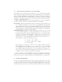
– →lts ⊆ Q×(Σ ∪R∪2C )×Q is the set of transitions, the smallest set respecting
the rules of Table 1.
a,φ
Action
Reset
Delay
l −→ l0 ν |= φ κ(l) = ∅
a
(l, ν) −→lts (l0 , ν)
κ(l) 6= ∅
κ(l)
(l, ν) −→lts (f ree(l), ν[κ(l)])
∀d0 ≤ d ν + d0 |= I(l) κ(l) = ∅
d
(l, ν) −→lts (l, ν + d)
Table 1. Transition relation of the labelled transition systems associated to a timed
automaton.
The definition we have given is different from the one usually in the literature
since we consider clock resets as external actions. The reason for this will become
clear later when we give semantics to our language and we want clock reset to
be visible; this makes no difference in our case because we use no relations based
on the labelled transition system (e.g, timed bisimulation); if we did, existing
results might not hold, but it would not be difficult to generalise the notions to
ignore clock reset actions.
The transition system defined above has an infinite (continuous) set of states
and actions; in order to be able to model check timed automata, we discretise
such state space into several equivalence classes that relate clock valuations that
agree on the integral part of clocks and on the ordering of their fractional part.
Let cx be the greatest constant against which clock x is compared, bxc the
integral part of x and f r(x) its fractional part. Given a set of clocks C, two clock
valuations ν and ν 0 are equivalent (ν ≡C ν 0 ) if all of the following conditions
hold:
– for all x ∈ C, bν(x)c = bν 0 (x)c or they both exceed cx ;
– for all x, y ∈ C, with ν(x) ≤ cx and ν(y) ≤ cy , f r(ν(x)) ≤ f r(ν(y)) if
f r(ν 0 (x)) ≤ f r(ν 0 (y));
– for all x ∈ C with ν(x) ≤ cx , f r(ν(x)) = 0 iff f r(ν 0 (x)) = 0.
A clock region is an equivalence class induced by ≡C , and the region graph
is the set of equivalence classes. Since all valuations in the same region agree on
the integral parts of the clocks, it is clear that the same set of action transitions
can be enabled from within the region. We denote the set of regions associated
to a timed automaton A by RA , and we let r, r1 , r2 . . . range over regions. We
also often denote a region by the set of clock constraints that are met by the
valuations in the region only. Finally, we denote by r0 the starting region (all
clocks set to 0) and by rmax the region for which x > cx for all clocks x.
With passage of time, the automaton changes region. Intuitively, we define
the successor region as the next region that the system will be in by letting time
elapse. Formally, the successor region is a function succ : R −→ R such that
succ(r) = r0 if for all ν ∈ r there exists d ∈ R such that ν + d ∈ succ(r) and for
all d0 < d either ν + d0 ∈ ν or ν + d0 ∈ succ(r). succ is undefined for rmax .
The action of moving to the next region involves an increment of the value
of all clocks, but only some of them actually cause the change of a region. For
example, if we consider two clocks x and y, when going from the region x = y = 0
to the region 0 < x = y < 1, both clocks change region. On the contrary, when
going from (0 < x < 1) ∧ (y = 0) to (0 < x < 1) ∧ (0 < y < 1) ∧ (y < x), it
is only y that changes region. We are interested in identifying the set of clocks
that change their own region as it will be convenient in the following.
We define clocks : R −→ 2C as the set of clocks that change their own region
at the next succ action; clocks(r) is the smallest set X of clocks such that for
all valuations ν ∈ r and η ∈ succ(r) we have ν ≡C\X η. We also define ∆ as the
set of actions describing the change of region; the elements of ∆ are δX , where
X ∈ 2C . We can now define the region automaton corresponding to a timed
automaton A.
Definition 2. Given a timed automaton A, the corresponding region automaton RA = (Qr , Σr , q¯r , →r ) is defined as follows:
–
–
–
–
Qr = {(l, r), l ∈ L ∪ f ree(L), r ∈ RA }
Σr = Σ ∪ ∆ ∪ 2C , with ∆ = {δX |X ⊆ C}
q¯r = (¯l, r0 )
→r ⊆ Qr × Σr × Qr such that:
a
a
• (l, r) −→r (l0 , r), a ∈ Σ if for all ν ∈ r, (l, ν) −→lts (l0 , ν);
X
X
• (l, r) −→r (l, r[X]), X ⊆ C if for all ν ∈ r, (l, ν) −→lts (l, ν[X]);
δX
d
• (l, r) −→r (l, succ(r)) if for all ν ∈ r there exists d such that (l, ν) −→lts
(l, ν 0 ) with ν 0 ∈ succ(r) and X = clocks(r).
Region automata are the basis for any algorithm to model check timed automata, and they are an important technique to discretise the infinite state
space of the induced transition system. Complexity is their main drawback, as
the number of regions is exponential in the number of clocks and constants. For
this reason, more efficient techniques have been devised (e.g. zones, see [Yov96]
for an introduction).
CSP CSP is a process algebra introduced by Tony Hoare [Hoa85]. It describes
concurrent systems in terms of their sequential components, characterised by the
sequences of actions that they can perform. CSP processes with action alphabet
Σ are generated by the following syntax:
P ::= ST OP | SKIP | a → P | P u P | P 2 P |
P || P | P \ A | f [P ] | µp.P | P ; P
A
where a ∈ Σ, A ⊆ Σ and f : Σ → Σ is a renaming function. The operators
above represent, respectively: deadlock, successful termination, action prefix,
internal choice, external choice, interface parallel, hiding, renaming, recursion
and sequential composition.
The semantics of a CSP term P is given by the set of actions that it can
perform (traces), by the set of actions that it can refuse after a possible trace
(failures) or by its possible infinite executions (divergences). Different relations
are built upon these semantic models: for each of them, equivalences between
processes are defined as set equalities; CSP also introduces the idea of refinement:
a process P1 is refined by another process P2 (P1 v P2 ) if every behaviour of
P2 is a possible behaviour of P1 , that is, if it is “less deterministic”. This idea is
formally defined as inverse set inclusion of traces, failures or divergences. For a
detailed introduction to CSP, see introductory texts, e.g. [Ros98] or [Sch99].
3
Clocked CSP
We define a language for describing timed automata, called Clocked CSP (CCSP),
as an extension of CSP, thus keeping its choice operators, the hiding operator
and the multi-way parallel composition. Clocked CSP terms with alphabet Σ
and set of clocks C are obtained by the following syntax:
P ::= ST OP | SKIP | (a, φ) → P | φ ..P | {|X|}P |
P 2 P | P u P | P || P | µp.P | P \ A | P ; P
A
where a ∈ Σ, A ⊆ Σ, φ ∈ B(C) and X ⊆ C. By convention, actions will be
ranged over by a, b, . . ., clocks by x, y, . . ., sets of clocks by X, Y, . . . and clock
constraints by φ, γ, · · · . We omit the interface alphabet of parallel composition
when implicit or not relevant. Most CSP constructs are kept unchanged; a few
have been modified in order to handle clocks:
– we have guarded actions: an action can be performed only when the condition
on the clocks is satisfied;
– we have a reset operation {|X|} that performs the resetting of the set of
clocks X to 0;
– we have an invariant operation .,
. corresponding to the idea of invariant of
timed automata.
3.1
Operational Semantics
Since Clocked CSP is designed to model timed automata, the operational semantics is intuitive and it extends CSP semantics in the obvious way.
For the purpose of giving semantics to Clocked CSP we introduce an extra
operator f ree(P ), representing a process that behaves exactly like P but which
does not perform any initial reset (i.e. the start state has been stripped of its
resets). We denote the set of all CCSP processes by CCSP and the set of all
CCSP processes with the f ree(•) operator by CCSP+ .
Given a CCSP term P , we define the corresponding timed automaton A(P ) =
(L, ¯l, Σ ∪ {τ }, C, I, κ, →), where L = CCSP+ , ¯l = P , the sets of clocks and
X
SKIP −→ Ω
a,ϕ
((a, ϕ) → P ) −→ P
a,ϕ
P −→ P 0
a,ϕ
{|X|}P −→ P 0
a,ϕ
0
P −→ P I(P ) = ϕ0
a,ϕ∧ϕ0
P 2 Q −→ P 0
τ,tt
P u Q −→ P
a,ϕ
P −→ P 0
a∈A
τ,ϕ
P \ A −→ P 0 \ A
µ,ϕ
P −→ P
µ∈
/A
µ,ϕ
P || Q −→ P 0 || f ree(Q)
a,ϕ
P −→ P 0
a,ϕ
P ; Q −→ P 0 ; Q
τ,tt
µp.P −→ P [µp.P/p]
a,ϕ
P −→ P 0
a,ϕ
ϕ ..P −→ P 0
a,ϕ
P −→ P 0
a,ϕ
f ree(P ) −→ P 0
τ,ϕ
0
P −→ P I(P ) = ϕ0
τ,ϕ∧ϕ0
P 2 Q −→ P 0 2 f ree(Q)
a,ϕ
P −→ P 0
f (a),ϕ
f [P ] −→ f [P 0 ]
µ,ϕ
P −→ P 0
µ∈
/A
µ,ϕ
P \ A −→ P 0 \ A
a,ϕ1 ,
a,ϕ
P −→
P 0 Q −→2 Q0
a∈A
a,ϕ1 ∧ϕ2
P || Q −→ P 0 || Q0
X
P −→ Ω
τ,tt
P ; Q −→ Q
I((a, ϕ) → P ) = tt
I(ϕ ..P ) = ϕ ∧ I(P )
I({|X|}P ) = I(P )
I(f ree(P )) = I(P )
I(P u Q) = I(P ) ∧ I(Q)
I(P 2 Q) = I(P ) ∨ I(Q)
I(P || Q) = I(P ) ∧ I(Q)
I(µp.P ) = ff
I(P \ A) = I(P ) I(f [P ]) = I(P ) I(P ; Q) = I(P )
κ((a, ϕ) → P ) = ∅
κ(ϕ ..P ) = κ(P )
κ({|X|}P ) = {X} ∪ κ(P )
κ(f ree(P )) = ∅
κ(P u Q) = ∅
κ(P 2 Q) = κ(P ) ∪ κ(Q)
κ(P || Q) = κ(P ) ∪ κ(Q)
κ(µp.P ) = ∅
κ(P \ A) = κ(P ) κ(f [P ]) = κ(P ) κ(P ; Q) = κ(P )
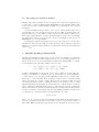
Table 2. Operational Semantics in terms of Timed Automata
actions are the same and κ, I and → are defined according to the rules of
Table 2 (note that for the binary operators 2 , u and ||, also the symmetric
rules hold). We have introduced the silent action τ , which is the result of some
internal computation, usually caused by internal choice or hiding. We have an
extra special label X (with no guard) to denote successful termination and an
extra process Ω that denotes the process that has successfully terminated.
In the following we will use the region automaton obtained from the operational semantics as the model we have in mind to define the denotational models
for CCSP. Given a CCSP term P and the associated timed automaton A(P ),
we denote the region automaton corresponding to A(P ) with initial region r
by R(P, r). If we want to add an extra invariant ϕ to the initial location (i.e.
I(P ) = I(P ) ∧ ϕ) , we denote the resulting region automaton by R(P, r, ϕ). We
use R(P ) as an abbreviation for R(P, r0 , tt).
3.2
A Denotational Semantics for Clocked CSP?
By working on the operational model defined above, one could use known equivalence relations for timed automata (e.g. timed bisimulation) or use traditional
model checking techniques to verify whether a given process meets some temporal logic property. Following the CSP tradition, we wanted to give a denotational
semantics to the language that would extend the usual trace/failures semantics
and lead to refinement relations.
While deciding what kind of denotational semantics to give to the language
we had to make several choices. We had in mind two main issues:
Decidability We want the refinement relations generated by the semantic model
to be decidable. Our aim is to be able to use or extend FDR2 to automatically
verify refinement for our processes. This excludes the use of timed traces,
that is, the traces obtained in the labelled transition system associated with
a timed automaton: it is known that timed trace inclusion and equivalence
are undecidable for timed automata [AD91].
Compositionality We want to be able to define the semantics of a process in
a compositional way, that is, to define the semantics of a composite process
in terms of its smaller components. This turned out to be not an easy task:
clocks can be seen as shared variables, so, when two processes execute concurrently (as the result of the parallel or external choice operators), one of
them can reset a clock, thus affecting the behaviour of the other process.
As an example, consider the following process:
P = {|x|}(a, x > 1) → ST OP
Q = (b, tt) → {|x|}(a, tt) → ST OP
R = P 2 (Q \ {b})
It is possible for process Q to reset the clock x after P has reset it and
started waiting for the guard x > 1 to become true. So, the behaviour
of P is influenced by Q’s internal actions, and it is not possible to define
P ’s semantics without knowing the context, placing some restrictions on
the processes and modifying the semantics. To avoid such problems, it was
necessary to impose several constraints on the syntax.
Our choice was to model the semantics on the region automaton. In the next
section we describe the trace semantics obtained by modelling region automata.
In the later sections we discuss advantages and disadvantages of our approach.
4
A Trace Semantics
In order to obtain compositionality, we have to impose restrictions on processes.
Since the interaction between processes that modify the value of clocks is
what creates most problems, we make the following simplification: each process
can handle only some clocks, so that its behaviour depends only on them. The
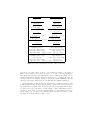
τ,ϕ
a,ϕ
P −→ P 0 I(P ) = ϕ0 P −→ P 0 I(P ) = ϕ0 κ(P 0 ) = ∅
a,ϕ∧ϕ0
τ,ϕ∧ϕ0
P 2 Q −→ P 0
P 2 Q −→ P 0 2 Q
τ,ϕ
0
P −→ P I(P ) = ϕ0 κ(P 0 ) 6= ∅
τ,ϕ∧ϕ0
P 2 Q −→ P 0
Table 3. New operational rules for external choice
other clocks are used by other processes that interact with it through the parallel
operator. More formally, for each process (or timed automaton), the set of clocks
C is partitioned into the set of internal clocks CI and the set of external clocks
CE . We restrict the parallel operator to work only on processes with distinct sets
of internal clocks.
The idea behind this is that, when defining the semantics of a term, we have
to assume any possible action on external clocks by the other processes, that is,
a process must be willing to synchronise on any possible set of (external) clock
reset at any moment. In this way processes always agree on the value of clocks.
This is the reason why we treat clock resets as visible actions: when a process
resets a set of clocks X, the other processes are willing to synchronise on this
reset actions and in this way they “know” what the other processes are doing.
We believe this is a reasonable restriction since in most examples involving timed
automata we have seen the requirement that parallel components use disjoint
sets of clocks.
The other critical operator is external choice, since processes involved can
take internal actions and then reset some clocks, thus modifying the behaviour of
the other component. This is another reason why we treat clock resets as external
actions that can resolve the choice. Informally, the idea is that, when presenting
the environment a choice, we present it under some conditions on clocks; we
therefore do not want a process to alter these conditions in a “hidden” way.
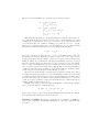
Table 3 reflects these new conditions on external choice by showing the modified
SOS rules for this operator.
Finally, we require the structure of a term to reflect the corresponding timed
automaton by having all clock resets and the invariants preceding the other operators (i.e. those enabling transitions). This can be achieved through syntactic
transformations that preserve the operational semantics.
4.1
The Semantic Model
We give Clocked CSP processes a semantics in terms of region traces. A region
trace is and element of RTraces = (Σ ∪∆∪2C )∗ , where Σ is the process alphabet,
∆ is the set of delay actions and C is the set of clocks. So an element of a trace
either denotes an action, the passage of time (delay action) or the reset of some
set of clocks.
We need to be able to define the semantics of a process from any possible
starting region and under any possible initial invariant. Consider for example the
process (a, x ≤ 1) → P : its semantics depends on the semantics of the process
P starting from 3 possible regions (x = 0, 0 < x < 1 and x = 1).
For this reason, the semantics of a process is the set of possible behaviours
under any possible starting condition. The refinement relation is extended accordingly as reverse set inclusion under every starting condition. Formally, let
R = {r1 , r2 , . . . , rn } be the set of regions corresponding to a term and Φ =
{φ1 , φ2 , . . . , φm } the set of possible invariants (note that this set is finite as an
invariant is the union of a set of regions). We define a function RT : CCSP ×
R × I → RTraces that returns the region traces of a process starting from a particular region under a particular invariant. The semantics of a process is given
by an ordered set of sets of traces.
RegionT races(P ) = (RT (P, r1 , φ1 ), RT (P, r1 , φ2 ), . . . , RT (P, r1 , φm ),
...
RT (P, rn , φ1 ), RT (P, rn , φ2 ), . . . , RT (P, rn , φm ))
The function RT is defined inductively on the syntax of terms along the same
lines as the definitions of the rules for traces for classical CSP. We can then
extend the refinement relation as reverse inclusion of behaviour:
P vRT Q iff RegionT races(P ) ⊇ RegionT races(Q)
iff ∀ri ∀φj RT (P, ri , φj ) ⊇ RT (Q, ri , φj )
that is, for every possible starting region, Q’s behaviour is a subset of P ’s behaviour. It can be shown that the refinement relation is independent of the
starting conditions for processes that reset all their clocks before referencing
them; in this way only one set inclusion needs to be verified. Moreover, we usually consider refinements between processes that have no external clocks, so that
their behaviour is self-contained.
Theorem 1. RegionT races is a monotonic function with respect to all the operators and the fixed-point operation is well defined for guarded processes.
Theorem 2. The function RT is a congruence with respect to the operational
semantics. That is, for all CCSP clock-closed terms P , regions r and invariants
ϕ, the following holds:
RT (P, r, I) = ΦT (R(P, r, I))
where ΦT (R(P, r, I) denotes the set of traces of the region automaton corresponding to process P under the given starting conditions.
One can easily expect the above result since we have modelled the trace
semantics on region automata, but it is still important as it allows us to perform model checking of refinement relations using the operational model as for
CSP [Ros94].
4.2
Extending the Semantics: Failures
Having defined the semantic model for region traces, the next natural step is
to extend it to a finer semantics that distinguishes between stable failures. We
define region failures, again having in mind the operational model of region
automata.
A region refusal set F is a subset of Σ ∪ ∆ ∪ 2C and it describes the set of
actions that a process can refuse after a given trace. The most interesting case
happens when a process refuses a delay action: it means that it refuses to let
time elapse; this is useful to describe timed liveness properties. A region failure
is a pair (t, F ), where t is a region trace and f is a refusal set. We denote by
RFailures the set of region failures.
Following the same ideas described above for region traces, we obtain a new
semantic model for Clocked CSP processes, given by a RegionF ailures function
which is once again congruent with the operational model, and a new refinement
relation vRF .
5
Model Checking Clocked CSP
At first, the semantics we have given does not seem very useful: one of its main
disadvantages is that it makes explicit references to clock names (syntactic entities) in the notion of trace and failure. In this way it distinguishes too much,
as it is shown in the following example: the processes
P1 = {|x|}(a, x = 1) → {|x|}(a, x = 1) → SKIP
P2 = {|x|}(a, x = 1) → (a, x = 2) → SKIP
would be distinguished as P1 resets clock x twice, while P2 does it only once.
Clearly, we would like to identify the two processes (they are timed bisimilar).
How can we overcome this problem? The first, trivial step is to define refinement “up to” clock renaming. Next, we have to define a way to verify interesting
timed properties. To do this, consider the trace model and note that if we hid
clock actions (either resets or delays) from traces we would be able to verify
functional (untimed) refinement. If we hid only some of them, then we would be
able to verify the refinement with respect to only a subset of clocks, possibly the
subset that describes the timed behaviour that we are interested in. We describe
the idea by means of an example (also used in [OW02]). Assume that we want
to check if a process respects the bounded invariance property
2(a ⇒ 2I ¬b)
where I = [0, n] is a closed interval starting from 0. This means that whenever
an action a is performed, the process cannot execute a b for the successive n
time units. This is a safety property that can be specified as a trace property.
The most non-deterministic process that respects this property is
S = (a, tt) → {|x|}S1 2
2 (c, tt) → S
c6=a
S1 = (a, tt) → {|x|}S1 2
2c6=a,b (c, x ≤ n) → S1 2
2 (c, x > n) → S
c6=a
This is the specification process against which processes are checked. To enable refinement another process is needed: in order to check whether a processes
P refines the specification S, we need to reset the clock x each time an action
a is performed. We can do this by defining a processes T = (a, tt) → {|x|} T ,
where x is a clock used only by T , i.e. it is an external clock for P , that performs
this function. The refinement that we need to check is the following:
S vRT
P || T
{a}
where the refinement is with respect to clock x only. This works because the
specification S does not allow the execution of any b before the value of clock
x is greater than n, and the passage of time is recorded by delay actions. Clock
hiding is defined as a combination of hiding and renaming on the set of traces
(and the operational model): if we hide a clock x, then we need to hide all the
reset or delay actions that involve it (or rename the action if other clocks are
reset or change region at the same time). This is why we add the information
of which clocks cause a region change to delay actions instead of having a single
generic delay action that would not allow hiding of clocks.
The trace model is enough to specify safety properties, as what is needed is
to include all those traces that do not present undesired behaviour. If we want
to verify liveness properties then we need to use the failures model. The idea is
the same as described above, that is, verify refinement with respect to only some
clocks. It would be possible to verify properties like strong bounded response by
defining additional processes as above.
Finally, it is possible to have successive refinements: considering the example
above, if the following two refinements hold
S vRT
P1 || T vRT
{a}
P2 || T
{a}
then both P1 and P2 respect the bounded invariance property and, in addition,
there is functional refinement between P1 and P2 .
Examples on FDR2: We have not tried the above examples on FDR2 because of the complexity of manually translating processes into equivalent CSP
processes.
We tested our ideas with small toy examples in the following way: firstly, we
defined small Clocked CSP processes, then we translated them into the equivalent timed automata and, from here, into the resulting region automata. At this
point we manually specified CSP processes equivalent to the region automata
and verified refinements between them with FDR2.
Given the complexity of building a region automaton, it would be desirable
to make the process above automatic.
Considerations: With the approach we have proposed we are able to verify
refinement between processes, and also both safety and liveness properties. More
importantly, timing aspects of processes are considered, possibly only those that
we are interested in.
Unfortunately, our approach has some disadvantages. One, and possibly the
biggest disadvantage is complexity: the number of regions corresponding to a
timed automaton is exponential in the number of clocks and size of constants;
this is carried over to our setting, making model checking possible only for small
systems, or systems with few clocks. Another smaller drawback is the fact that
we have to manually specify process specifications, as we did for the example
above. It would be interesting to find a way to automatically generate such
processes from some an appropriate logic.
6
Conclusions
In this paper we have described a proposal for a timed extension to CSP, called
Clocked CSP. We have defined its semantics and the corresponding refinement
relations, showing how it would be possible to use the model checker FDR2 to
verify such relations, and also some timed properties of systems. Possible future
work will be aimed at improving the complexity of model checking, investigating
whether it possible to use known efficient techniques for timed automata in our
case; it would also be interesting to define a logic that could be verified with
our technique. Finally, we plan to compare our approach with other similar
approaches to extending CSP with real time in more details.
References
[ACD93] R. Alur, C. Courcoubetis, and D.L. Dill. Model-checking in dense real-time.
Information and Computation, 104(1):1–34, 1993.
[AD91] R. Alur and D. Dill. The theory of timed automata. In J.W. de Bakker,
C. Huizing, W.P. de Roever, and G. Rozenberg, editors, Proceedings of the
REX Workshop “Real-Time: Theory in Practice”, volume 600, pages 45–73,
1991.
[D’A99] P. R. D’Argenio. Algebras and Automata for Timed and Stochastic Systems. PhD thesis, Department of Computer Science, University of Twente,
November 1999.
[DJR+ 92] J. Davies, D. Jackson, G. Reed, J. Reed, A. Roscoe, and S. Schneider.
Timed csp: Theory and practice. In Proceedings of REX Workshop, Nijmegen, LNCS 600, Springer-Verlag, 1992., 1992.
[For93]
Formal Systems (Europe) Ltd. Failures divergence refinement — user manual
and tutorial, 1993. Version 1.3.
[Hoa85] C.A.R. Hoare. Communicating Sequential Processes. Prentice-Hall International, Englewood Cliffs, 1985.
[Jac92]
D. M. Jackson. Logical Verification of Reactive Software Systems. PhD
thesis, University of Oxford, 1992.
[LPY97] Kim G. Larsen, Paul Pettersson, and Wang Yi. Uppaal in a Nutshell. Int.
Journal on Software Tools for Technology Transfer, 1(1–2):134–152, October
1997.
[Mil89]
R. Milner. Communication and Concurrency. Prentice-Hall International,
Englewood Cliffs, 1989.
[Oua01] Joël Ouaknine. Discrete Analysis of Continuous Behaviour in Real-Time
Concurrent Systems. PhD thesis, 2001.
[OW02] Joël Ouaknine and J. B. Worrel. Timed CSP = Closed Timed Automata.
In Proceedings of EXPRESS 02, 2002.
[Ros94] A.W. Roscoe. Model-checking CSP. In A Classical Mind: Essays in Honour
of C.A.R. Hoare. Prentice Hall, 1994.
[Ros98] A.W. Roscoe. Theory and Practice of Concurrency. Prentice Hall, 1998.
[RR86]
G.M. Reed and A.W. Roscoe. A timed model for communicating sequential
processes. In Proceedings of ICALP 86, pages 314–323. Springer LNCS, 1986.
[Sch97] Steve Schneider. Timewise refinement for communicating processes. Science
of Computer Programming, 28(1):43–90, 1997.
[Sch99] S. Schneider. Concurrent and Real-time Systems: The CSP Approach. John
Wiley and Sons, 1999.
[Yov96] Sergio Yovine. Model checking timed automata. In European Educational
Forum: School on Embedded Systems, pages 114–152, 1996.
[Yov97] Sergio Yovine. Kronos: A verification tool for real-time systems. (kronos
user’s manual release 2.2), 1997.
[YPD94] W. Yi, P. Pettersson, and M. Daniels. Automatic verification of real-time
communicating systems by constraint-solving. In Proc. of the 7th International Conference on Formal Description Techniques, 1994.