1
Modelling tips for Times∗
19 November 2003
This document will help newcomers to Times to get started with modelling and verification. It is
assumed that you have access to the User Manual1 . This document covers Times version 1.2β.
Learning T IMES
Times is based on timed automata with tasks, that is finite state machine extended with clocks,
data variables and executable tasks. A system in Times is composed of concurrent processes, each
modelled as an automaton. An automaton is constructed using locations connected with edges.
A state of the system is determined by the current location of each process and the values of the
clocks and data variables. A transition from one state to the next follows an edge in one or two
processes and updates the variables according to the assignment label(s) of the edge(s).
To control when to fire a transition, it is possible to use guards and synchronizations. A guard is
a condition on the variables and the clocks saying when a transition is enabled. The synchronization mechanism in Times allows two processes to perform a hand-shaking synchronisation. If
two processes have enabled transitions with complementary synchronisation labels, e.g. a! and
a?, they may take a compound transition. In a synchronisation both processes will change location
simultaneously. When taking a transition actions may be performed. Three types of actions are
possible: assignments of variables, resets of clocks and release of tasks.
Clocks are special types of variables that are used in Times to measure time. Time is continuous and all clocks have the same rate. The clock variables can be tested in guards on edges
and they may also be reset when a transition is taken. It is important to note that the clocks are
real-valued even though we may only test them against discrete values.
Tasks A task in Times is an executable piece of code annotated with parameters, such as worst
case execution time and priority. When a task is executed it performs a computation or interacts
with the hardware. It is assumed that the tasks are reliable and have a well known behaviour.
Templates Each process in a system is an instance of a template. A template consists of an
automaton with locations, edges, guards and actions. The template also has formal parameters
that can be replaced with actual channels, variables, constants and clocks when the template is
instantiated as a process. The motivation for the templates is that systems often have several
processes that are very alike.
Note the difference between processes and tasks. Processes execute concurrently and are
described using automata. Tasks are released by the processes to execute separately. We can can
view an executing system as consisting of two execution units as illustrated in Figure 1. One
where the processes execute in parallel and one where the tasks are executed.
The rest of this document explores some key points of Times through examples.
∗ This
1 The
document is based on Alexandre DAVID:s Uppaal2k: Small Tutorial
User Manual is available at http:\\www.timestool.com
1
Figure 1: Processes and tasks.
Mutual Exclusion Algorithm
As our first exercise, we study Petterson’s mutual exclusion algorithm to see how we can derive
a model as an automaton from a program/algorithm and check properties related to it.
The algorithm for two processes is as follows in C:
Process 1
req1=1;
turn=2;
while(turn!=1 && req2!=0);
//critical section
job1();
req1=0;
Process 2
req2=1;
turn=1;
while(turn!=2 && req1!=0);
//critical section
job2();
req2=0;
A global variable reqn is associated with each process. When a process want to enter the
critical section it sets its req variable. The protocol also uses the global variable turn that helps
the processes to alternate their access to the critical section so they get a fair share. In the while
statement the process loops until the other process has left the critical section (if it was there).
Notice that the protocol is symmetric, so we may use a template of Times and create two
instances of it. On our way towards a model of the algorithm we also observe that the algorithm
has four states, we mark them with a notation similar to goto labels as follows:
Process 1
idle:
req1=1;
want:
turn=2;
wait:
while(turn!=1 && req2!=0);
CS:
//critical section
job1();
//and return to idle
req1=0;
We are only interested in the control structure, not in the work done in the critical section, so
we abstract that part of the algorithm. Now, create a new template called mutex and draw the
automaton depicted in Figure 2.
Note how the condition in the while statement turn!=1 && req2!=0 is converted into the
guards on the edges from Wait to Critical Section. We need to use two separate edges since Times
cannot handle guards with disjunctions.
2
Figure 2: Mutex template
Figure 3: Instantiation of two processes based on the template Mutex.
The template is instantiated with three parameters, two integers bounded between 0 and 1
and one constant. Enter them by typing int[0,1] req1; int[0,1] req2; const me in
the Parameters field.
To create the instances open the Project tab and add two processes and choose the template
to create them from. Name the first process P1 and give it the parameters req1, req2, 1 and
name the second P2 with parameters req2, req1, 2, as shown in Figure 3. In the figure you
can also see how the global variables have been declared as: int[0,1] req1, int[0,1] req2
and int[1,2] turn.
You have now modelled the algorithm by defining templates, instantiating them and declaring variables. Now choose Simulation in the Run menu. In the simulator view you can simulate your system by choosing an enabled transition and clicking the “Step forward” button ([]B).
Try to reach the critical section in both processes at the same time . . . well you cannot, you may
also use the verifier to make sure of this.
Verification Choose Verification... in the Run menu. Enter the mutual exclusion property: A[] not (P1.Critical_Section and P2.Critical_Section) and press the OK
3
Figure 4: Error trace from faulty Mutex model illustrated in the Simulator.
button.2 The verifier should answer with ’SATISFIED’. If the answer were ’NOT SATISFIED’
it means that the property does not hold, but that should not be the case for this property.
The property A[] is a safety property: you check that not (P1.Critical_Section and
P2.Critical_Section) is always true. Another type of properties, reachability properties
start wit the quantifier E<> instead. For example, enter a new property E<> P1.Critical_Section,
that checks if process P1 may reach the location corresponding to the critical section.
Diagnostic traces If the result of a verification is negative Times can return a diagnostic trace.
To see how first change the model so it is faulty. For example change the guard req2==0 to
req2==1. Then choose Configuration... in the Options menu and make sure that the
the check-box Generate Trace is checked on the Verifier tab. Now run the verification
property again. This time it should not be satisfied and you will get a dialog window with an
option to show the trace, click the “Show Trace”-button to go to the simulator. In Figure 4 the
simulator is shown where the error trace is loaded. You can use the simulator to examine the
found trace.
Tasks and Scheduling in T IMES
We continue our presentation of Times by discussing how to use tasks. A task in Times can have
either periodic or controlled arrival patterns. A periodic task is simply added to the task table and
the period is given. For controlled tasks we use automata to specify when the task should be
released. Each location in an automaton may have an associated task and when the location is
entered the task is released to the task queue.
Times lets us choose a scheduling strategy for the task queue, for example fixed priority scheduling, earliest deadline first or rate monotonic. The scheduling strategy is used by Times when it performs simulation, verification and schedulability analysis.
2 Note
that spaces in names of locations and processes are replaces by underscores ( _ ).
4
Figure 5: Automaton controlling tasks P and Q.
Figure 6: One possible schedule for the system in Figure 5 with EDF scheduling strategy.
As an exercises we will create a simple automaton controlling the releases of two tasks. Open
a new system and add two controlled tasks P and Q to the task table. Set their parameters as in the
table below:
Name
P
Q
Computation time
3
4
Deadline
10
7
Create a new template and draw an automaton like the one shown in Figure 5, where x is
a local clock. The automaton will control the release of the instances of the tasks. Initially task
P is released, then after 3 time units the automaton may proceed to Location 2 where task Q is
released. Since task P has computation time 3, the queue is empty when task Q is released. In
Location 2 the automaton may after 5 time units loop back and release task Q again, or return to
Location 1 and release task P.
We can study the behaviour of the system in the simulator where the Message Sequence Chart
(MSC) view in the upper right panel helps us see how the automaton executes. The MSC will
include two extra automata: SCHEDULER and PERIODIC_TASKS. These are created automatically by Times based on the selected scheduling strategy to control the execution of the released
tasks.
When we simulate we will also see new locations named REL_P_1 and REL_Q_1 in the process we created (Process_1). These are auxiliary locations introduced by Times to handle the
release of tasks.
In the panel below the MSC we can see how the tasks are scheduled in a Gantt chart. One
possible schedule where earliest deadline first (EDF) is used as scheduling strategy is shown in
Figure 6.
To verify that the model is schedulable we can use one of the main features of Times, namely
schedulability analysis. Choose the scheduling strategy you want to use in the task table and
choose Schedulability analysis in the Run menu. Times will answer ’SATISFIED’, this
simple example is schedulable with all the available scheduling strategies.
Precedence constraints
Sometimes it is important that tasks execute in a given order. This is for example the case when
the output of one task is used as input to another task.
5
Figure 7: Example of cyclic precedence graph.
In Times we may define precedence constraints in the Precedence tab in the editor. The precedence constraints are described using one or more graphs. The nodes of the graph(s) represent
tasks and the edges represents precedence relations. An ordinary precedence relation applies to
all task instances and is denoted with a solid-line arrow. An inter-iterative precedence relation
applies to all task instances except the first one and is denoted with a dashed arrow (99K). An
example of precedence graph is shown in Figure .
According to the graph task P4 can start its execution only if it is preceded by P3 and P5 and
either P1 or P2. The first instance of P1 can start its execution at any time while any further
instances must be preceded by task P4. P3 can start executing only when P2 has finished, and
any further instances of P2 must be preceded by an instance of P3.
Time in T IMES
We continue with a more in-depth discussion of the concept of time in Times. We will explain
the concepts through examples. You are encouraged to draw the examples and make your own
experiments.
The first and most important fact about time in Times is that it is continuous. One may be
confused by the fact that it is only compare clocks with integer constants, such as x > 5, but we
should think of the clocks as being able to have all values between the integers also.
It is also important to know that the clock values are not repy
resented explicitly in the verifier or the simulator. Instead they
are represented symbolically as zones. For example the time in a
state could be defined as that clock x is between 2 and 4 and clock
y is between 3 and ∞. For the simple case with only two clocks
7
we may represent this zone as in Figure 8.
6
5
4
Experiments
3
To get
further understanding of how time is handled in Times we will study the simple automaton 2shown in Figure 9(a). We will use a single clock x. We also use the observer shown in Figure
x
9(b)1 for the following experiments.
The channel reset is used for synchronization between the
observer and the automaton when the clock reaches 2.
1 2 3 4 5 6
Normally an observer is an add-on automaton in charge of detecting events without perturbing the observed system. Our observer does in fact interact with the system since the reset of
Figure 8: Zone representing
the clock (x:=0) is delegated to the observer. This modification does not modify the original
the values of clocks x and y.
behaviour of the simple automaton but is necessary to make all steps in the behaviour accessible
for simulation and verification.
Draw the model, name the automata P1 and Obs and instantiate them in the project tab.
Notice that the state Taken of the observer is of type committed that is both transitions are taken
as one atomic action. Declare the channel with chan reset; in the global variables section. If
you only simulate the system you may not detect all the important details of the behaviour.
6
(a) Simple automaton
(b) Observer
4
clock x
Figure 9: Simple timed automata and observer
2
2
4
6
8
"time"
Figure 10: Time behaviour of first example: this is one possible run.
Instead we will use queries to the verifier and progressively modify the system. The expected
behaviour of our system is depicted in Figure 10.
Try these properties to exhibit this behaviour:
• A[] Obs.Taken imply x>=2 : all resets of the clock value (see curve) are above 2. This
query means: for all states, being in the location Obs.Taken implies that x>=2.
• E<> Obs.Idle and x>3 : this is for the waiting period, you can try values like 30000
and you will get the same result. This question means: is it possible to reach a state where
Obs is in the location Idle and x>3.
4
clock x
From these queries we learn a very important fact. If a guard is enabled it does not mean that
the transition have to be taken. That is we must explicitly tell the system that is should make
progress!
To ensure progress we may use invariants. Add the invariant x<=3 to the Loop location as
shown in Figure 11. The invariant is a progress condition: the system is not allowed to stay in
2
2
4
6
8
Figure 11: Adding an invariant: the new behaviour.
7
"time"
clock x
4
2
2
4
6
8
"time"
Figure 12: No invariant and new guard.
the location when the invariant is false, so the transition have to be taken and the clock reset in
our example.
To see the difference from before, try the properties:
• A[] Obs.Taken imply (x>=2 and x<=3) to show that the transition is taken when
in the interval 2-3.
• E<> Obs.Idle and x>2 : it is possible to take the transition in the interval 2-3.
• A[] Obs.Idle imply x<=3 : to show that the upper bound is respected.
The former property E<> Obs.Idle and x>3 no longer holds.
Remove the invariant and change the guard to x>=2,x<=3. You may think that it is the same
as before but it is not! The system has no progress condition, just a new condition on the guard.
Figure 12 shows the modified system.
As you can see the system may take the same transitions as before, but there is now a possible
deadlock: the system may get stuck if it does not take the transition within 3 time units.
To see what happens retry the same properties, the last one does not hold now. You can see
the deadlock with the following property: A[] x>3 imply not Obs.Taken, that is after 3
time units the transition is not taken any more. Another alternative is to use the property A[]
not deadlock, that is not satisfied either.
Urgent/Committed Locations
We will now look at the different kinds of locations of Times. You already saw the type committed in the previous example. There are three different types of locations in Times: normal locations (with or without invariants), urgent locations and committed locations. Draw the automata
depicted in Figure 13 in three different templates. Define the clocks x locally in each template.
8
Figure 13: Automata with normal, urgent and committed locations.
Name the automata Pnormal, Purgent and Pcommited respectively. The state marked U is
urgent and the one marked C is committed. Try them in the simulator and notice that when in the
committed location, the only possible transition is always the one leading out of the committed
location. Committed locations are used to define atomic sections within an automaton. When the
atomic section is started no other automaton may take a transition until this automaton reaches
a non-committed location.
To see the difference between normal and urgent states, use the verifier to try these properties:
• E<> Pnormal.L1 and Pnormal.x>0 : it is possible to wait in L1.
• A[] Purgent.L1 imply Purgent.x==0 : it is not possible to wait in L1.
Time may not pass in an urgent state, but interleavings with normal states are allowed as you
can see in the simulator.
Verification properties
In the examples above we have used the verifier several times to check for properties of a model.
We will now give a more complete treatment of properties we can check using the verifier.
Basically the verifier of Times can search for the existence or absence of properties of the
model. The properties are defined with so called state formulas, that is logical formulas defining a
state of the system. The elements of the formulas can be:
• Location in a process, like: Process1.Location
• Condition on a local variable, like: Process.Var == 5
• Condition on a global variable, like: x < 2
A formula can be combined using the operators or, and, not and imply and grouped using
parenthesis. An example of a non-trivial state formula is (P1.L1 imply (x>2 or y>2))
which should be interpreted as: whenever process P1 is in location L1 the variable x or the variable y is larger than 2. This is of course totally different from for example ((P1.L1 imply
x>2) or y>2).
The verifier can search for state formulas in different ways. We will use path quantifiers to
choose how. In the previous we have used the reachability quantifier (E<>) and the invariant
quantifier (A[]). These are the two simplest types of path quantifiers available.
9
The reachability quantifier tells the verification algorithm to search for a path of transitions
that leads to a state where the formula holds. If such a path exist the whole quantified formula
is satisfied. If it does not hold the verification algorithm will have searched the whole state space
and we know that the formula does not hold anywhere.
The invariant quantifier tells the verification algorithm to check if the state formula holds
everywhere. We can view this as the inverse of the reachability property. That is, if A[] p holds
then not E<> not p also holds.
The verification engine of Times also understands a couple of other path quantifiers. In summary, the queries available in the verifier are:
Possibly
E<> p: there exists a path where p eventually hold.
Invariantly
A[] p: for all paths p always hold, equivalent to: not E<> not p
Potentially always E[] p: there exists a path where p always hold.
Eventually
A<> p: for all paths p will eventually hold, equivalent to: not E[] not p.
Leads-to
p --> q: whenever p holds q will eventually hold, equivalent to: A[] (p
imply A<> q) .
Deadlock
A[] not deadlock : The system can not deadlock.
where p and q are state formulas. The full grammar of the query language is available in the User
Manual. Note the useful special form A[] not deadlock that checks for deadlocks.
We see that some of the formulas can be expressed in terms of each other. In fact only E<>
and E[] are really necessary. In the in-formal definition of these properties that we give below
we use (Ln , vn ) to stand for a state, where Ln denotes the current location of all processes and vn
denotes the variable values. We also use Inv(Ln ) to stand for the invariant of location Ln .
Possibly The property E<> p evaluates to true for a timed transition system if and only if there
is a sequence of transitions s0 → s1 → . . . → sn , where s0 is the initial state and sn satisfies p.
Potentially always The property E[] p evaluates to true for a timed transition system if and
only if there is a sequence of transitions s0 → s1 → . . . → si → . . . for which p holds in all states
si and which either:
• is infinite, or
• ends in a state (Ln , vn ) such that
– either for all d: (Ln , vn + d) satisfies p and Inv(Ln ), or
– there is no outgoing transition from (Ln , vn )
Modeling Tricks
Finally we have collected some useful modelling tricks that can make your life as a Times-user
much easier.
Urgent channels and urgent transitions Times offers urgent channels that are synchronizations
that must be taken when the transition is enabled without delay. Clock conditions on these transitions are not allowed. It is possible to encode “urgent transitions” by using urgent channels. Use
a dummy process with one location and a loop labelled with the urgent channel go!. To make a
transition urgent in another automaton, add a synchronisation on go? as shown in Figure14.
10
Figure 14: Encoding urgent transitions using urgent channels
Value passing in synchronisations Times does not directly support value passing in synchronisations, but this can easily be encoded using a shared variable: define a global variable x, and
use it to write and read the passed value as in Figure 15. It is also possible to write the receive
statement on a single edge like this: read? y:=x;.
Figure 15: Value passing using global variable x.
Broadcast and multicast The current version of Times does not support broadcast or multicast
communication: synchronization is only between pairs of automata. Instead, you can encode
multicast using a series of committed locations. The sending automaton would have a sequence
of locations like in Figure 16 and each receiving automaton an edge with the corresponding
go1?, go2? and go3?. Several solutions are possible.
Figure 16: Multicast.
State-space explosion Verifying a large model can take a long time and use up large amounts
of memory. To keep a model manageable, one has to pay attention to some points:
• The number of clocks has an important impact on the complexity, so use as few as possible.
• The use of committed locations can significantly reduce the state space. But you have to be
careful not to take away relevant interleavings of states.
• The number of variables plays an important role as well, and more importantly their range.
Whenever possible you should define a range for the variables as we have done in the
examples above. In particular, avoid unbounded loops on integers since the values will
then span over the full range.
Periodic tasks A tasks can be declared to be periodic with a period T in the task table. Such
tasks cannot be released by automata but are handled by the automatically created process PERIODIC_TASKS. Another way to declare periodic tasks is to declare the task as controlled and create
an automaton like the one shown in Figure 17.
11
Figure 17: Controlled periodic task.
Task with varying period A semi-periodic tasks where the period varies within a range cannot
be declared in the task table. Instead we must use an automaton to control the task. Assume that
a task arrives non-deterministically with an interval between 10 and 20 time units. An automaton
that releases the task Q in this fashion is shown in Figure .
Figure 18: Controlled semi-periodic task.
Locked locations In some cases a task must finish before the controller can continue. This is for
example the case when the task reads a sensor value that the controller uses. The following trick
makes use of the task interface to lock the controller in a location until the task finishes.
Declare a global boolean variable int[0,1] TaskDone and edit the interface of the task
to set the variable to TaskDone:=1. Then we can lock the controller to the location until R is
finished by adding the labels to the edges leading out of the location as shown in Figure 19. Note
that the transition is made urgent using the trick with an urgent channel go? presented above.
Figure 19: Automaton locked until task R is done.
References
[YPD94] Wang Yi, Paul Pettersson, and Mats Daniels. Automatic Verification of Real-Time Communicating Systems By Constraint-Solving. In Proc. of the 7th International Conference on
Formal Description Techniques, 1994.
[LPY95] Kim G. Larsen, Paul Pettersson, and Wang Yi. Model-Checking for Real-Time Systems.
In Proc. of Fundamentals of Computation Theory, volume 965 of Lecture Notes in Computer
Science, pages 62–88, August 1995.
[JLS96]
H.E. Jensen, K.G. Larsen, and A. Skou. Modelling and Analysis of a Collision Avoidance
Protocol Using SPIN and U PPAAL. In Proc. of 2nd International Workshop on the SPIN
Verification System, pages 1–20, August 1996.
[LPY97] Magnus Lindahl, Paul Pettersson, and Wang Yi. Formal Design and Analysis of a GearBox Controller: an Industrial Case Study using U PPAAL. In preparation, 1997.
[AD94] R. Alur and D. Dill. A Theory for Timed Automata In Theoretical Computer Science,
volume 125, pages 183–235, 1994.
12