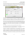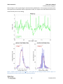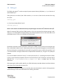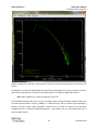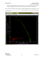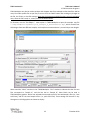
1
TOPO Version 2.2 Installation Guide & User’s Manual 7 October 2013 Copyright © 1997 – 2013 David L. Windt [email protected] TOPO Version 2.2 Preface This document is the place to go for help with TOPO. It is meant to be a combination Installation Manual (Chapter 1), Quick-Start Guide (Chapter 2), Tutorial (Chapter 3) and Reference Manual (Chapter 4), with a few examples included in Chapter 3 to illustrate some of TOPO’s capabilities. TOPO was originally developed as a library of IDL routines to be used in your own IDL programs for analysis of measured 1D and 2D surface topography data obtained from optical surfaces. This version of TOPO is focused principally on enhancements made since the last release to the user-friendly programs included along with the TOPO IDL routines: these programs are (now) called TOPO_prof, TOPO_psd, and TOPO_surf. There’s also a new program called TOPO*Multiplot, for analyzing one or more 2D surface data files. Each of the user-friendly programs use a graphical user interface (GUI), and can be run as-is (for example directly from the TOPO Launcher program) for a variety of analyses of topography data, without having to write new IDL programs. I hope you will read Chapters 1 and 2 of this document to get TOPO installed and running properly on your computer. After that, Chapter 3 of this document is a tutorial on the use of the GUI-based TOPO routines, with examples demonstrating some of their capabilities, while Chapter 4 is a reference manual for the TOPO IDL routines that you can use in your own IDL programs. Also, check out the IMD & TOPO Google group (https://groups.google.com/forum/#!forum/imd_topo) for discussion, and announcements of future releases. A note about notation Throughout this manual computer file names are always written in this font. When files are written with their full path (or sometimes even with a partial path, as in the very next sentence), I’ll use notation applicable to unix (i.e., linux, Mac OS X, and Solaris) operating systems, using a forward slash (/) to delineate subdirectory names. For example: “…/topo/examples”, which means the examples subdirectory in the topo installation directory; the leading “…/” means “wherever the topo installation directory is installed on your computer”. Of course Microsoft Windows platforms use the backward slash (\), as in “…\topo\examples”, so if you’re using a Windows computer, please substitute backward slashes for forward slashes when you see a file name with a forward slash in this document. Acknowledgements The on-going development of TOPO has been made possible in large part by continual support from NASA, since 1999, for highenergy astrophysics technology development, most recently under NASA grant number NNX13AC54G. To all the NASA people involved, and the proposal review panels over the years: I can’t thank you enough for your support! I also wish to thank to all the TOPO users who have provided to me valuable feedback and suggestions. 2 7 October 2013 TOPO Version 2.2 TOPO Version 2.2 Installation Guide & User’s Manual Contents 1 Installing TOPO ...................................................................................................................................... 6 1.1 1.1.1 Using TOPO as an IDL application ......................................................................................... 6 1.1.2 Using TOPO as an XOP extension .......................................................................................... 6 1.2 Installing TOPO as an IDL application............................................................................................ 7 1.3 Installing TOPO as an XOP extension .......................................................................................... 10 1.4 Customizing the TOPO installation: topo_cfg.pro............................................................... 12 1.4.1 Non-standard installation location ..................................................................................... 12 1.4.2 Other customizable settings ............................................................................................... 12 1.5 2 3 4 System Requirements ................................................................................................................... 6 Common Installation Problems and Solutions ............................................................................ 13 Using TOPO ......................................................................................................................................... 14 2.1 Overview: What is TOPO and what can it do? ............................................................................ 14 2.2 Starting TOPO.............................................................................................................................. 15 TOPO Launcher Programs ................................................................................................................... 16 3.1 TOPO_prof .................................................................................................................................. 16 3.2 TOPO_psd ................................................................................................................................... 21 3.3 TOPO_surf ................................................................................................................................... 24 3.4 TOPO*Multiplot .......................................................................................................................... 27 TOPO for IDL Programmers................................................................................................................. 39 4.1 TOPO Common Block Variables .................................................................................................. 39 4.2 Data-Importing Routines............................................................................................................. 40 4.2.1 EROM .................................................................................................................................. 40 3 7 October 2013 TOPO Version 2.2 4.2.2 RD_MICROMAP ................................................................................................................... 42 4.2.3 RD_NANOSCOPE ................................................................................................................. 42 4.2.4 RD_WYKO_TOPO3D ............................................................................................................ 43 4.2.5 RD_ZYGO_NEWVIEW .......................................................................................................... 44 4.3 TOPO Launcher (GUI) Routines ................................................................................................... 44 4.3.1 TOPO_prof .......................................................................................................................... 44 4.3.2 TOPO_psd............................................................................................................................ 46 4.3.3 TOPO_surf ........................................................................................................................... 47 4.3.4 TOPO*Multiplot .................................................................................................................. 48 4.4 Computational and Graphics Routines ....................................................................................... 49 4.4.1 ANGLE2WAVES.................................................................................................................... 49 4.4.2 ANLZ_PROF ......................................................................................................................... 50 4.4.3 AUTOCOV_FIT ..................................................................................................................... 52 4.4.4 AUTOCOV2PARS .................................................................................................................. 53 4.4.5 AUTOCOV2PSD .................................................................................................................... 54 4.4.6 HEIGHT_DIST ....................................................................................................................... 54 4.4.7 PARS2AUTOCOV.................................................................................................................. 55 4.4.8 PARS2PSD ............................................................................................................................ 56 4.4.9 PLOT_AUTOCOV .................................................................................................................. 57 4.4.10 PLOT_H_DIST....................................................................................................................... 58 4.4.11 PLOT_PROF.......................................................................................................................... 59 4.4.12 PLOT_PSD ............................................................................................................................ 60 4.4.13 PLOT_S_DIST ....................................................................................................................... 61 4.4.14 PLOT_SLOPE ........................................................................................................................ 62 4.4.15 PROF2AUTOCOV ................................................................................................................. 63 4.4.16 PROF2PSD ........................................................................................................................... 64 4.4.17 PROF2SLOPE........................................................................................................................ 65 4.4.18 PSD_FIT ............................................................................................................................... 65 4.4.19 PSD_FIT_OMEGA_NU_N ..................................................................................................... 66 4.4.20 PSD_FIT_SIGMA_XI_H ......................................................................................................... 67 4.4.21 PSD2AUTOCOV.................................................................................................................... 68 4 7 October 2013 TOPO Version 2.2 5 4.4.22 PSD2PARS ............................................................................................................................ 69 4.4.23 PSD2RAVEPSD ..................................................................................................................... 69 4.4.24 PSDPARS_ANGLE2SIGMA_L ................................................................................................ 70 4.4.25 PSDPARS2SIGMA_L ............................................................................................................. 71 4.4.26 SUB_TILT ............................................................................................................................. 72 4.4.27 SURF2AVE_PSD ................................................................................................................... 72 4.4.28 SURF2PSD ............................................................................................................................ 73 4.4.29 TOPO_X_CONVERT.............................................................................................................. 75 4.4.30 TOPO_Y_CONVERT .............................................................................................................. 75 Performance and Troubleshooting ..................................................................................................... 77 5.1 5.1.1 Q: I can’t get TOPO to work/start. ...................................................................................... 77 5.1.2 Q: Can I get a copy of the TOPO source code? ................................................................... 77 5.1.3 Q: Will/can you include feature X in a future release of TOPO? ........................................ 77 5.1.4 Q: Will TOPO work with the free IDL Virtual Machine? ...................................................... 77 5.2 6 Frequently Asked Questions ....................................................................................................... 77 Reporting Bugs ............................................................................................................................ 77 References .......................................................................................................................................... 79 5 7 October 2013 TOPO Version 2.2 1 Installing TOPO 1.1 System Requirements TOPO is written in the IDL scientific programming language, and will run on any platform supported by IDL. While most TOPO routines are intended for use in your own IDL programs, the GUI-based programs included with TOPO – TOPO_prof, TOPO_psd, TOPO_surf, and TOPO*Multiplot – require little or no IDL expertise. There are two ways to run TOPO: (1) using a licensed copy of IDL, and (2) using the free XOP package, which includes an embedded, licensed copy of IDL. 1.1.1 Using TOPO as an IDL application TOPO can be run using IDL version 6.3 or higher. IDL is available for purchase from Exelis Visual Information Solutions: http://www.exelisvis.com/ProductsServices/IDL.aspx NOTE: The full version of IDL is required to run TOPO. TOPO will NOT run using the free IDL Virtual Machine. 1.1.2 Using TOPO as an XOP extension TOPO can be run as an ‘extension’ to the free XOP software package, available at ESRF: http://www.esrf.eu/Instrumentation/software/data-analysis/xop2.3 If you will use TOPO as an XOP extension, you can run the GUI-based TOPO programs to analyze surface topography data. You will not be able to use your own IDL programs containing TOPO routines, however. 6 7 October 2013 TOPO Version 2.2 TOPO Installation Guide 1.2 Installing TOPO as an IDL application If you will use TOPO as an XOP extension, then you can skip this section and proceed to §1.3. Once you have IDL installed and running on your computer, follow these steps to install and run TOPO: 1. Create a directory (folder) called user_contrib in the main IDL installation directory. NOTE: You can install TOPO in a different directory if you so choose. But if you do not install TOPO in the user_contrib directory as described here, then you must edit the topo_cfg.pro configuration file to specify the actual installation location. See §1.4.1 for further details. 2. Download the TOPO installation file topo_xxx.tar.gz from http://www.rxollc.com/idl/ (xxx=version number; for example, topo_2.2.tar.gz) 3. Unpack the topo_xxx.tar.gz file containing the topo installation directory. • For Windows: use a program like Winzip to open topo_xxx.tar.gz • For Linux/Mac OS X/Solaris: use the gunzip command: $ gunzip topo_xxx.tar.gz followed by the tar command: $ tar –xvf topo_xxx.tar 4. Move the TOPO installation directory to the user_contrib directory created in step 1. (i.e., to …/idl/user_contrib/topo) 5. Start IDL and add the new user_contrib directory just created in step 1 to your IDL search path. Consult the IDL documentation for help configuring the IDL_PATH environment variable. If setting IDL_PATH manually, be sure to include a “+” sign so that the subdirectories under user_contrib will be included (e.g., IDL_PATH=+/usr/local/rsi/idl/user_contrib:…) If you’re using IDL’s Preferences GUI to set the search path, be sure to check the ‘search subdirectories’ box: 7 7 October 2013 TOPO Version 2.2 TOPO Installation Guide 6. After your IDL search path has been redefined in step 5, type .run topo at the IDL prompt to start TOPO: 8 7 October 2013 TOPO Version 2.2 TOPO Installation Guide 7. The TOPO splash-screen will appear. Click ‘OK’ to start TOPO Launcher and load the TOPO library of IDL routines. From TOPO Launcher you can run the GUI programs TOPO*Multiplot, TOPO_prof, TOPO_psd, and TOPO_surf: 8. You’re up and running! Now please read the rest of TOPO.pdf so that you get the most out of TOPO! Also, check out the IMD & TOPO Google group (https://groups.google.com/forum/#!forum/imd_topo) for discussion, and announcements of future releases. 9 7 October 2013 TOPO Version 2.2 TOPO Installation Guide 1.3 Installing TOPO as an XOP extension If you will NOT use TOPO as an XOP extension, then you can skip this section and proceed to §1.4. Once you have XOP installed and running on your computer, follow these steps to install and run TOPO: 1. Download the TOPO installation file topo_xxx.tar.gz from http://www.rxollc.com/idl/ (xxx=version number; for example, topo_2.2.tar.gz) 2. Unpack the topo_xxx.tar.gz file containing the topo installation directory. • For Windows: use a program like Winzip to open topo_xxx.tar.gz • For Linux/Mac OS X/Solaris: use the gunzip command: $ gunzip topo_xxx.tar.gz followed by the tar command: $ tar –xvf topo_xxx.tar 3. Move the topo installation directory to the extensions directory in the XOP installation directory (e.g., to …/xop2.3/extensions/topo). 4. For Windows only: • copy the file C:\xop2.3\extensions\topo\extras\topo4xop.bat to C:\xop2.3\topo4xop.bat and • copy the file C:\xop2.3\extensions\topo\extras\topo4xop.vbs to C:\xop2.3\topo4xop.vbs The name of the XOP installation directory depends on the version of XOP that you have installed, and on where you have installed it on your computer. For this step we’ve assumed that XOP V2.3 is installed in the default location C:\xop2.3. However, if you have a different version of XOP, or a different installation location, please substitute the correct name and path for your XOP installation directory above. Note: if you don’t use the default installation location (C:\xop2.3), you MUST edit topo4xop.bat and specify the correct path to xop.bat. You might also want to make a shortcut on your Desktop to one or both of these files, so you can start TOPO by double-clicking that shortcut. Use topo4xop.vbs if it works on your system, otherwise use topop4xop.bat. 5. Start TOPO: • For Windows: Double-click on topo4xop.vbs (or topo4xop.bat if necessary.) Or, start XOP and then use the XOPLoad extension… menu option to select topo4xop. • For Linux/Mac OS X/Solaris: At the command line, type: xop topo4xop 10 7 October 2013 TOPO Version 2.2 TOPO Installation Guide 6. The TOPO splash-screen will appear. Click ‘OK’ to start TOPO Launcher. From TOPO Launcher you can run the GUI programs TOPO*Multiplot, TOPO_prof, TOPO_psd, and TOPO_surf: 7. You’re up and running! Now please read the rest of TOPO.pdf so that you get the most out of TOPO! Also, check out the IMD & TOPO Google group (https://groups.google.com/forum/#!forum/imd_topo) for discussion, and announcements of future releases. 11 7 October 2013 TOPO Version 2.2 TOPO Installation Guide 1.4 Customizing the TOPO installation: topo_cfg.pro 1.4.1 Non-standard installation location If you will use TOPO with a licensed copy of IDL, and you choose not to install the TOPO installation directory in the default location, i.e., the user_contrib directory in the main IDL directory as described in §1.2, then you must edit the TOPO configuration file topo_cfg.pro, which is located in the topo installation directory you have selected: specifically, using any plain-text editor, change the value of the topo_home variable defined in this file so that it refers to the actual location where you’ve installed the topo directory on your computer. EXAMPLE: You are using a linux system and you have installed topo in your home directory, e.g., /users/joe/topo. Edit topo_cfg.pro and replace the line if (!version.os_family eq 'unix') then topo_home=!dir+’/user_contrib/topo/’ with if (!version.os_family eq 'unix') then topo_home=’/users/joe/topo/’ 1.4.2 Other customizable settings There are other operating-system- and site-specific settings that you can modify in the topo_cfg.pro configuration file, specifically those that control the fonts and special characters used by the TOPO graphical user interfaces (GUI). Please follow the instructions contained within the topo_cfg.pro file to make such modifications. If you are using TOPO on a unix platform, you can also use the Xdefaults configuration file included in the topo/extras directory to set some TOPO-specific X-windows preferences. One method to do this is to copy the contents of topo/extras/Xdefaults into your personal .Xdefaults file, or into the IDL Xdefaults file, !dir/resource/X11/lib/X11/app-defaults/Idl, where !dir is the IDL installation directory on your computer. 12 7 October 2013 TOPO Version 2.2 TOPO Installation Guide 1.5 Common Installation Problems and Solutions Problem: IDL can’t find TOPO: IDL> .run topo Error opening file. File: TOPO Solution: You must add the TOPO installation directory to your IDL search path, as described in §1.2. Problem: The TOPO windows don’t look right, and/or don’t look much like the examples in this document. Solution: The fonts used by TOPO, which are specified in the topo_cfg.pro configuration file, might not be available on your computer. Edit the topo_cfg.pro file, as described in §1.4, and specify valid fonts that are actually installed on your computer. i Problem: Special characters, such as ‘Å’, ‘µ’, ‘δ’, etc., don’t display correctly in the TOPO windows. Solution: The special character codes for your particular installation, which are specified in the topo_cfg.pro configuration file, must be the correct codes for the fonts used by TOPO, which are also specified in that file. Edit the topo_cfg.pro file, as described in §1.4, and specify valid special character codes for the fonts that you have specified.i i If your operating system is not specifically listed in the topo_cfg.pro configuration file, you’ll need to manually add the necessary entries for optical constants and atomic scattering factors directories, fonts, etc, using as a template the lines in that file that contain “YOUR OS”: replace “YOUR OS” with the value of the IDL system variable !version.os as defined on your computer. 13 7 October 2013 TOPO Version 2.2 2 Using TOPO 2.1 Overview: What is TOPO and what can it do? The TOPO software package comprises a library of IDL routines for analysis of measured 1D or 2D surface topography data, such as that obtained by atomic-force-microscopy (AFM), optical profilometry, or any other type of contact or non-contact surface profile measurement technique. The TOPO routines are largely based on the work by Bennet and Mattsson, 1 and Church, 2 and you are strongly encouraged to read the material in those references; only minimal discussion is included in this document of the concepts behind the TOPO surface topography analysis routines. The TOPO IDL routines can be used in your own IDL programs, if you are running TOPO as an IDL application. TOPO also includes four user-friendly programs, each with a graphical user interface (GUI): TOPO_prof, for analysis of 1D surface height (profile) data; TOPO_psd, for analysis of 1D powerspectral-density (PSD) data; TOPO_surf, for analysis of 2D surface height data; and TOPO*Multiplot, for analysis of one or more 2D surface height data sets. The TOPO GUI programs can be executed from TOPO Launcher, or from the IDL command line (if you are use TOPO as an IDL application). 14 7 October 2013 TOPO Version 2.2 TOPO User’s Manual 2.2 Starting TOPO Follow the instructions in Chapter 1 to install TOPO on your computer. To start TOPO, follow these steps, as appropriate for your installation: Operating System IDL or XOP Any IDL Linux/Mac OS X/ Solaris XOP Windows XOP Starting IMD Start IDL and then type IDL> .run topo You can also re-start TOPO Launcher by typing ‘topo_launcher’ at the prompt: IMD> topo_launcher At the command line, type $ xop topo4xop Or, type $ xop and then XOPLoad extension… and then select topo4xop from the list of installed extensions, and then click ‘Accept’. Double-click ii C:\xop2.3\topo4xop.vbs If that doesn’t work Double-click C:\xop2.3\topo4xop.bat If neither method works, edit topo4xop.bat and check that the specified path to xop.bat is correct for your installation. Or, start XOP (as per the XOP instructions) and then XOPLoad extension… and then select topo4xop from the list of installed extensions, and then click ‘Accept’. ii Replace C:\xop2.3 with your actual XOP installation directory. 15 7 October 2013 TOPO Version 2.2 3 TOPO Launcher Programs This chapter is meant to be a brief tutorial on the stand-alone, user-friendly programs included in the TOPO library that can be run from TOPO Launcher. These programs also can be run directly from the IDL command line, or called from your own IDL programs, if you are running TOPO as an IDL application. There is no limit on the number of instances of any of these programs that can be opened simultaneously. Detailed reference information for IDL programmers regarding the TOPO Launcher routines described in this chapter, along with reference information on the underlying TOPO IDL routines used by these programs, is presented Chapter 4. The routines included in the TOPO library that can be used to read topography data files are also described in Chapter 4. Note: The “FileChange Working Directory…” menu option in TOPO Launcher allows you to globally change the working directory. It is equivalent to using the IDL ‘cd’ command at the IDL prompt. 3.1 TOPO_prof The TOPO_prof program iii is used to analyze 1D surface profile data, i.e., surface height, Y, as a function of surface position, X. TOPO_prof can be run directly from TOPO Launcher, or it can be run from the IDL command line using the syntax: IDL>topo_prof Or, if you have already defined X and Y: IDL>topo_prof,x,y Note: The X and Y variables must be one-dimensional arrays of equal length, both defined in units of angstroms. The X values also must be equally spaced. When first starting TOPO_prof from TOPO Launcher, or from the command line without passing X and Y values (i.e., first command-line example above), you will be prompted to enter an IDL command to read profile data stored in a file, so as to define the X and Y arrays: iii TOPO_prof is essentially a wrapper for the ANLZ_PROF routine described in §4.4.2. IDL Programmers should consult §4.3.1 for more information on the TOPO_prof routine. 16 7 October 2013 TOPO Version 2.2 TOPO User’s Manual 3.TOPO Launcher Programs The default command to read 1D profile data in TOPO_prof is ‘EROM’, which can be used to read plain text files, as described in detail in §4.2.1. Alternatively, you can use your own IDL programs to read 1D profile data, by entering the corresponding IDL commands, using valid IDL syntax, to define the variables X and Y, into the text-box in the figure shown above. Compound IDL commands (i.e., using the “&” symbol) are allowed. If you use the default command “erom,x,y” to read a plain text file (i.e., containing two columns of data, X and Y), you will then be prompted to select the name of the file to read. To illustrate, we’ll open the 1D profile-data file ‘…/topo/examples/profile_data_example.txt’ that is included with the TOPO distribution: After opening the surface profile data file, TOPO_prof displays by default (a) a plot of Y as a function of X, with the peak-to-valley (P-V) and rms roughness (σ) values computed from the profile data indicated on the plot; (b) plots of the surface height and surface slope distributions, with Gaussian fits and best-fit widths displayed, (c) a plot (and fit) of the autocovariance function computed from the X,Y profile data, and (d) a plot (and fit) of the power-spectral-density (PSD) function computed from the X,Y profile data. 17 7 October 2013 TOPO Version 2.2 TOPO User’s Manual 3.TOPO Launcher Programs The TOPO Profile Analysis window is shown in Figure 1 as it appears just after opening the example file mentioned above. Figure 1. TOPO_prof window after opening the example file described above. 18 7 October 2013 TOPO Version 2.2 TOPO User’s Manual 3.TOPO Launcher Programs You can uncheck the boxes near the top of the TOPO Profile Analysis window to suppress display of any of the plots. You can adjust the appearance of each plot, and control how any fit may be displayed in that plot, using the corresponding options in the Preferences menu. For example, here’s the window that appears after selecting “PreferencesPower-Spectral-Density…”: The controls at top of this particular window are used to specify how the PSD is computed from the profile data (i.e., frequency range used for PSD computation, zero padding, and windowing, as per §4.4.16), and if a power-law fit is displayed or not. The controls at bottom are used to adjust the appearance of the plot. Preferences windows associated with the other types of plots work similarly. The Units menu on the main TOPO_prof window can be used to display lengths and/or heights in units of Å, nm, µm, or mm, while the Precision menu controls the number of digits displayed to the right of the decimal point for length, height and slope parameters displayed on any plots. Note that these settings are global, and thus affect the display of any TOPO graphics, not just those displayed in TOPO_prof. The “FileOpen…” menu option can be used to open a different data file in TOPO_prof. You can export profile data, as well as the computed height histogram, slope histogram, autocovariance function and PSD function, using the corresponding “FileExport ____....” menu options. You can print a hardcopy of the displayed graphics, or print the graphics to a file, using the “FilePrint…” menu option. For example, you can print to a PostScript (.ps) file, which can then be converted to any number of other graphics file formats using freely available programs (such as GhostScript, ImageMagick, etc.), or imported into vector graphics programs (such as Corel Draw, Adobe Illustrator, etc.) for conversion and/or further manipulation. To illustrate, shown in Figure 2 is a graphic that was made from a PostScript file that was created by printing from the TOPO_prof window shown 19 7 October 2013 TOPO Version 2.2 TOPO User’s Manual 3.TOPO Launcher Programs above in Figure 1, after suppressing the autocovariance and PSD plots; in this example the PostScript file was imported into CorelDraw and then exported as a JPEG, for import into the Word document used to create the PDF you are now reading. Figure 2. Graphics produced using the “FilePrint…” menu option from the TOPO_prof window shown in Figure 1. A PostScript file was created and then converted to JPEG using CorelDraw. 20 7 October 2013 TOPO Version 2.2 TOPO User’s Manual 3.TOPO Launcher Programs 3.2 TOPO_psd The TOPO_psd program iv is used to analyze 1D power-spectral-density (PSD) data, i.e., S, as a function of spatial frequency, F. TOPO_psd can be run directly from TOPO Launcher, or it can be run from the IDL command line using the syntax: IDL>topo_psd or, if you have already defined F and S: IDL>topo_psd,f,s Note: S and F must be one-dimensional arrays of equal length; S has units of Å3, while F has units 1/Å. When first starting TOPO_psd from TOPO Launcher, or from the command line without passing F and S values (i.e., first command-line example above), you will be prompted to enter an IDL command to read profile data stored in a file, so as to define the F and S arrays: The default command to read 1D PSD data in TOPO_psd is ‘EROM’, which can be used to read plain text files, as described in detail in §4.2.1. Alternatively, you can use your own IDL programs to read 1D profile data, by entering the corresponding IDL commands, using valid IDL syntax, to define the variables F and S, into the text-box in the figure shown above. Compound IDL commands (i.e., using the “&” symbol) are allowed. If you use the default command “erom,f,s” to read a plain text file (i.e., containing two columns of data, F and S), you will then be prompted to select the name of the file to read. To illustrate, we’ll open the 1D PSD-data file ‘…/topo/examples/PSD_x_example.txt’ that is included with the TOPO distribution. After opening the surface profile data file, the TOPO PSD Analysis window displays by default the data and a power-law fit (described in Church [2]): iv TOPO_psd is essentially a wrapper for the PLOT_PSD routine described in §4.4.12. IDL Programmers should consult §4.3.2 for more information on the TOPO_psd routine. 21 7 October 2013 TOPO Version 2.2 TOPO User’s Manual 3.TOPO Launcher Programs Options available from the TOPO_psd menu bar are similar to those described above for the TOPO_prof routine. As explained in §4.3.2, the TWOD keyword to the TOPO_psd procedure can be set to indicate that the F and S values correspond to a 1D slice of a 2D PSD function, or a radially-averaged PSD function. Note: When TWOD is set, S must be defined in units of Å4. If the TWOD keyword has been set, or if you start TOPO_psd by clicking the button labeled “TOPO_psd: 1D power-spectral-density analysis (/TWOD)” on TOPO Launcher, then the PSD fit-type displayed by default is the Ω/ν/n PSD model, explained in Stearns et al. [3]. Other fit options for 2D PSD data, available from the “PreferencesAxis/Fitting/Style…” menu option, are the σr/ξ/H PSD model [4], as well as a power-law [2]. 22 7 October 2013 TOPO Version 2.2 TOPO User’s Manual 3.TOPO Launcher Programs Note: The best-fit parameters derived using the Ω/ν/n or the σr/ξ/H PSD models in TOPO using radially-averaged PSD data can be used to define the PSD of a surface or interface in IMD. Here’s the TOPO_psd window after opening the radially-averaged PSD data contained in the file ’…/topo/examples/PSD_r_example.txt’, with the default Ω/ν/n fit and best-fit parameter values displayed: 23 7 October 2013 TOPO Version 2.2 TOPO User’s Manual 3.TOPO Launcher Programs 3.3 TOPO_surf The TOPO_surf program v is used to analyze 2D surface profile data, i.e., surface height, Z, as a function of surface position, X and Y. TOPO_surf can be run directly from TOPO Launcher, or it can be run from the IDL command line using the syntax: IDL>topo_surf or, if you have already defined X, Y and Z: IDL>topo_surf,x,y,z Note: The X and Y variables must be one-dimensional arrays, both defined in units of angstroms. The Z variable must be a two-dimensional array (whose dimensions correspond to those of X and Y), defined in units of angstroms. When first starting TOPO_surf from TOPO Launcher, or from the command line without passing X, Y, and Z values (i.e., first command-line example above), you will be prompted to enter an IDL command to read surface data stored in a file, so as to define the X, Y and Z arrays: The default command to read 2D profile data in TOPO_surf is ‘RD_NANOSCOPE’, which can be used to read an AFM image created by the Brücker/Veeco/Digital Instruments Nanoscope III instrument, as described in detail in §4.2.3. Other routines built-in to TOPO for reading surface profile data files are described in §4.2. Alternatively, you can use your own IDL programs to read 1D profile data, by entering the corresponding IDL commands, using valid IDL syntax, to define the variables X, Y, and Z into the textbox in the figure shown above. Compound IDL commands (i.e., using the “&” symbol) are allowed. To illustrate, we’ll use the default RD_NANOSCOPE routine to open the 2D surface-data file ‘…/topo/examples/nanoscope_example_6_v_0x05120005.dat’ that is included with the TOPO distribution: v IDL Programmers should consult §4.3.3 for more information on the TOPO_surf routine. 24 7 October 2013 TOPO Version 2.2 TOPO User’s Manual 3.TOPO Launcher Programs The TOPO Surface Analysis window after opening this example file is shown in the next figure. The Peak-to-Valley and RMS roughness values are displayed at the top left. You can use the check-box and text-box at the bottom to subtract a polynomial from the image, e.g., to remove piston, tilt, sphere, etc. offsets from the data. As you move the mouse over the image, the Z value is also displayed at the 25 7 October 2013 TOPO Version 2.2 TOPO User’s Manual 3.TOPO Launcher Programs top, and X and Y profiles are plotted in the windows below and to the left of the image, respectively. You can left-click to “capture” an X profile (row), and right-click to capture a Y profile (column). Here’s how the window appears after we’ve captured two X profiles and one Y profile; we’ve also adjusted the color table using the “PreferencesAdjust Color Table…” menu option: Captured profiles are shown in the list located in the middle of the window, and the corresponding surface profile and 1D PSD’s are displayed in the plots on the right. If a profile in the list is selected – the 2nd profile in the list is selected in the above figure – you can click the “Analyze Profile” button to display the selected profile in a new TOPO_prof window. You can also export to plain text files the selected 1D profile data, and the corresponding 1D PSD data, using the buttons labeled “Export Profile” and “Export PSD”, respectively. (You can also export the profile data sent to TOPO_prof using that program’s “FileExport Profile…” menu option described above.) The menu options “AnalysisRadially-Averaged PSD…” and “AnalysisX- and Y-Averaged PSD…” can be used to compute from the 2D surface data the radially-averaged PSD (using the SURF2PSD §4.4.28 and PSD2RAVEPSD §4.4.23 routines) and the X- and Y-averaged PSDs (i.e., the average of all the 1D PSDs computed from each row or column of the image, respectively, using the SURF2AVE_PSD routine, §4.4.27), which are then displayed in new TOPO_psd windows; these quantities can then be exported to plain text files from TOPO_psd. 26 7 October 2013 TOPO Version 2.2 TOPO User’s Manual 3.TOPO Launcher Programs 3.4 TOPO*Multiplot The TOPO*Multiplot routine is used to analyze and visualize one or more 2D surface data files. TOPO*Multiplot can be run directly from TOPO Launcher, or it can be run from the IDL command line using the syntax: IDL>topomultiplot When TOPO*Multiplot is first started, it looks like this: Each 2D surface data file to be included for display in TOPO*Multiplot must be added one at a time. Click on the little “Files…” button at the bottom of the TOPO*Multiplot window (circled in red in the figure above) to open the “TOPO*Multiplot – Files” window associated with this instance of TOPO*Multiplot, shown in the next figure: 27 7 October 2013 TOPO Version 2.2 TOPO User’s Manual 3.TOPO Launcher Programs To add a new surface-data file, click the “Add File” button circled in red above. (We’ve already clicked it in the figure above.) Then enter the IDL command to read the data file in the text-box labeled “IDL Read Command:”. You can use one of the routines described in §4.2, or your own IDL routines if running TOPO as an IDL application. Specify the name of the file to read in the text-box labeled “File:”. Click the button labeled “Read” to import the file. TOPO*Multiplot will read the data file specified, and also compute the height histogram, the 2D PSD, the 1D radially-averaged PSD, and the 1D X- and Y-averaged PSDs. To illustrate, Figure 3 shows the “TOPO*Multiplot - Files” window after loading the same Nanoscope image we used in §3.3. 28 7 October 2013 TOPO Version 2.2 TOPO User’s Manual 3.TOPO Launcher Programs Figure 3. The “TOPO*Multiplot - Files" window after loading a surface-data file. Displayed below the “File:” text-box in the “TOPO*Multiplot - Files” window shown above is information regarding the contents of the file: in this case, the file contains a 512x512 image, measured over an area 2 µm x 2 µm on Aug 19 2005. The next row of controls, starting with the check-box labeled “Only use surface data between”, can be used to ignore surface data outside the Z-range you specify. (For example, if your AFM image includes a piece of dust, you can limit the heights used to compute the PSD etc., so that the dust is not included.) The next row down contains the controls used to determine how the PSD functions are computed. (See, e.g., §4.4.28.) The Radially-Averaged PSD, the X-Averaged PSD, and the Y-Averaged PSD functions can each be displayed in a separate TOPO_psd window by clicking the corresponding “Plot” buttons (that look like this: ); these computed functions can also be exported as plain text files by clicking the corresponding “Export” buttons (that look like this: ). The row of controls with the “Plot Style” label are used to adjust the display of any 1D functions (e.g., Height Histograms and PSDs) that you may choose to plot in TOPO*Multiplot, as we’ll explain below. The next row shows the P-V and RMS roughness values computed from the surface data (included any limits on Z you may have specified); the check-boxes can be used to include these values in TOPO*Multiplot 29 7 October 2013 TOPO Version 2.2 TOPO User’s Manual 3.TOPO Launcher Programs graphics, as we’ll also explain below. The last row includes four text-boxes where you can enter (X,Y) or (R, Phi) position values; these quantities are meant to refer to the measurement location on the sample surface, and are only used for plot labels and legends, as we’ll explain. After loading a surface data file following the procedure just described, return to the main TOPO*Multiplot window and click the “Refresh” button. By default, a 2D contour of the image will be displayed, as in the next figure (where we’ve also set Length units to µm): 30 7 October 2013 TOPO Version 2.2 TOPO User’s Manual 3.TOPO Launcher Programs The drop-list labeled “Plot Type:” circled in the previous figure is used to select the type of plot displayed, with a variety of other options. For example, the next figure shows the Radially-Averaged PSD computed from this same data: There are a variety of controls to adjust the plot appearance (e.g., titles, axes ranges, grid lines, etc), and additional controls specific to the type of plot being displayed. The button labeled “Add Plot” (circled in red above), can be used to create new tabs on the TOPO*Multiplot window, and each plot tab can display a different type of plot. The example 31 7 October 2013 TOPO Version 2.2 TOPO User’s Manual 3.TOPO Launcher Programs TOPO*Multiplot file “…/topo/examples/topomultiplot_example_1_measurement.tmp” contains the same surface data we’ve used in the example above, and has been configured with four different plot tabs, to illustrate some of TOPO*Multiplot’s visualization capabilities. (The tabs were also re-named, using the button labeled “Rename”.) To open this .tmp file, use the “FileOpen…” menu option on the TOPO*Multiplot menu bar. The last three tabs are shown in the figures below: 32 7 October 2013 TOPO Version 2.2 TOPO User’s Manual 3.TOPO Launcher Programs 33 7 October 2013 TOPO Version 2.2 TOPO User’s Manual 3.TOPO Launcher Programs 34 7 October 2013 TOPO Version 2.2 TOPO User’s Manual 3.TOPO Launcher Programs TOPO*Multiplot can also be used to analyze and compare data from multiple surface data files. Add as many 2D surface profile files as you like; be sure to click the ‘Read’ button after making any changes to the file, the Z limits, or the PSD settings. Note that the histogram and PSD functions are only computed once, when the file is read, i.e., when you click the ‘Read’ button. To illustrate, use the “FileOpen…” menu option in TOPO*Multiplot to open the example .tmp file “…/tmp/examples/topomultiplot_example_4_measurements.tmp”, which contains four AFM images from two different samples; each sample was measured over 2 µm and 10 µm scan lengths: We’ve used the “Label:” text box in the “TOPO*Multiplot - Files” window to indicate that the first two files correspond to “Sample A”, and the last two to “Sample B”; these labels can be used in TOPO*Multiplot graphics. We’ve also selected the same plot styles for the two Sample A files (i.e., blue solid lines), and for the two Sample B files (i.e., pink solid lines). These settings will be used in any Histogram or 1D PSD graphics we choose to display. 35 7 October 2013 TOPO Version 2.2 TOPO User’s Manual 3.TOPO Launcher Programs One plot tab on the main TOPO*Multiplot window in this example .tmp file has been configured to display all four AFM images in a 2x2 grid; a second plot tab displays the radially-averaged PSDs computed from each image. Here’s how those two tabs appear (after setting the background to white, using the “Screen ColorBlack on White” menu option): 36 7 October 2013 TOPO Version 2.2 TOPO User’s Manual 3.TOPO Launcher Programs We’ve checked the box labeled “Condensed” in the last figure above: this causes the plot legend to display just a single line for Sample A, and a single line for Sample, in blue in pink, respectively. If the “Condensed” box is unchecked, the legend would include a line for each of the 4 files included in the list shown in the “TOPO*Multiplot - Files” window. (That might be useful, in this particular example, to distinguish between the 2 µm and 10 µm scans as well as the sample IDs, if we had configured the 2 µm scans to display using other colors, or dotted lines, perhaps.) We’ve also checked the “Date” box in the above example, which causes the measurement dates to be included in the legend. If you specify (X,Y) or (R,Phi) location values for each file, these values can also be included in the legend by checking the corresponding boxes. 37 7 October 2013 TOPO Version 2.2 TOPO User’s Manual 3.TOPO Launcher Programs After you’ve configured TOPO*Multiplot to your liking, you can save the results to a .tmp file using the “FileSave…” menu option. Note: When you save a TOPO*Multiplot file, all surface data loaded into TOPO*Multiplot are included in the .tmp file. The “FilePrint…” menu option can be used to print a hardcopy of each plot tab. You can also print to a PostScript file to create graphics that can be used for presentations or publications. For example: Figure 4. Graphics produced using the “FilePrint…” menu option from the TOPO*Multiplot window shown in the previous figure: a PostScript file was created and then converted to JPEG using CorelDraw. 38 7 October 2013 TOPO Version 2.2 4 TOPO for IDL Programmers 4.1 TOPO Common Block Variables If you are using TOPO as an IDL application, then you will have started TOPO at the IDL command line, using “.run topo”, as explained in Chapter 2. Some TOPO routines use IDL common block variables, which are defined and accessible at the command line when you run topo.pro this way. Almost none of these common block variables should be used directly in your own IDL programs, but you need to know their names in order to avoid inadvertent problems, e.g., by using variables having the same names in your own IDL commands and programs. In any case, the TOPO routines uses a common block called TOPO, defined as follows: COMMON TOPO,TOPO,TOPO_HOME,TOPO_BM The TOPO variable defined in the TOPO common block is an IDL structure variable, and is the only common block variable that may be of use to you when writing your own IDL programs that use TOPO routines. The TOPO variable structure tags that you can use are those that control the display of length and height variables, and of length-, height-, and slope-related parameters. That is, all surface data – i.e., Y(X) and Z(X,Y) – must be defined in TOPO in units of angstroms. However you can display surface data, and surface-derived quantities (i.e., height and slope histograms, and PSD and autocovariance functions, along with fits to those functions) in TOPO graphics routines using units of Å, nm, µm, or mm. Units can be controlled using the menu options in the TOPO Launcher programs described in the previous chapter. Or, displayed units can be controlled directly by setting the TOPO.XUNITS_PTR and TOPO.YUNITS_PTR structure tags at the command line or in your own IDL programs: TOPO.XUNITS_PTR: An integer that defines the length units for displayed variables. Set this variable to 0 for angstroms, 1 for nm, 2 for microns, and 3 for mm. TOPO.YUNITS_PTR: An integer that defines the height units for displayed variables. Set this variable to 0 for angstroms, 1 for nm, 2 for microns, and 3 for mm. The precisions with which best-fit parameters and other quantities (e.g., RMS roughness, etc.) are displayed are controlled by the TOPO.XPRECISION, TOPO.YPRECISION, and TOPO.SPRECISION structure tags: TOPO.XPRECISION: An integer that defines the number of digits displayed to the right of the decimal point for length-related parameters (e.g., correlation length.) TOPO.YPRECISION: An integer that defines the number of digits displayed to the right of the decimal point for height-related parameters (e.g., RMS roughness.) 39 7 October 2013 TOPO Version 2.2 TOPO User’s Manual 4. TOPO for IDL Programmers TOPO.SPRECISION: An integer that defines the number of digits displayed to the right of the decimal point for slope-related parameters (e.g., RMS slope.) 4.2 Data-Importing Routines The IDL routines described in this section can be used to read 1D or 2D surface data files in TOPO. You can also use your own IDL programs to read surface data files, if you are using TOPO as an IDL application. If you are using TOPO as an extension to XOP, then these are likely to be the only routines you can use to import your measured surface data. The source code for the EROM procedure is included with the ‘windt’ library, at www.rxollc.com/idl.The source code for the remaining data-importing routines described here is included in the ‘…/topo/readers’ directory. 4.2.1 EROM NAME: EROM PURPOSE: Read columns of data from a text file. This program can be used to read data written by the MORE program. The file to be read must be such that if the data are space-separated, then all variables are numeric; String variables are allowed only if the data are separated by tabs, colons, etc. The file may contain any number of comment lines - which MUST begin with a semicolon, and MUST be positioned before all data lines. CALLING SEQUENCE: EROM,V0[,V1,V2,...V9] or EROM,V=V KEYWORD PARAMETERS: V - Set this keyword to a named variable that will be returned as an array of structures holding the data and the variable names specified in the last comment line. See RESTRICTIONS below for more details. FILE - String specifying the name of a file; if not supplied, the user is queried. SKIP - The number of lines at the beginning of the file that should be skipped. TAB - Specify /TAB for tab-separated data. (The default is spaceseparated data.) It is only necessary to specify this keyword if the file contains any string data columns. SEPARATOR - A string specifying the character separating the data columns. 40 7 October 2013 TOPO Version 2.2 TOPO User’s Manual 4. TOPO for IDL Programmers COMMENT - Set this keyword to a named variable that will be returned as a string array holding the comment lines included in the file. GROUP - GROUP_LEADER keyword passed to DIALOG_PICKFILE if FILE is not specified. CANCEL - Set this keyword to a named variable that will be returned to indicate if the user pressed the CANCEL button when prompted for a file to read, if the FILE keyword is not set. OUTPUTS: If the V keyword is not used, then the user must specify the correct number of Vi (V0, V1, etc.) output parameters. There must be as many Vi's specified in the call to EROM as there are columns of data. The V's are double-precision arrays, unless either the TAB or SEPARATOR keyword is specified in which case they are all string arrays. RESTRICTIONS: If EROM is called with the V keyword, then the columns of data contained in the file are returned as double-precision fields in the returned V structure variable. Use of the V keyword requires that the data file contain at least one comment line, and the last comment line MUST include the names of the data variables separated by the "|" character. For example, to read a file using the V keyword containing three columns of 10 rows of data, then the last comment line in the file must look like this: ; First Variable Name | Second One | Another Variable Name Thus the V structure returned by EROM will have the following tag names: HELP,/STR,V V[0].VALUE V[0].NAME V[1].VALUE V[1].NAME V[2].VALUE V[2].NAME DOUBLE STRING DOUBLE STRING DOUBLE STRING Array[10] 'First Variable Name' Array[10] 'Second One' Array[10] 'Another Variable Name' MODIFICATION HISTORY: David L. Windt, Bell Labs, March 1990 January, 1997 - DLW Modified to ignore lines beginning with semicolons, and to accept data separated by tabs, etc.; Removed the NOTITLE and COMMENT keyword; included PICKFILE to prompt for filenames when not specified. June, 1997 - DLW Returned numeric variables are now double-precision instead of floating-point. DLW, May 2003 Added V, COMMENTS, GROUP and CANCEL keywords. Replaced call to PICKFILE with call to DIALOG_PICKFILE 41 7 October 2013 TOPO Version 2.2 4.2.2 TOPO User’s Manual 4. TOPO for IDL Programmers RD_MICROMAP NAME: RD_MICROMAP PURPOSE: Read a Micromap data file. CALLING SEQUENCE: RD_MICROMAP,FILE=FILE,X,Y,Z KEYWORD PARAMETERS: FILE - name of Micromap data file. TILT_SUB - set to subtract tilt. SPHERE_SUB - set to subtract a 2nd order polynomial background. HIST_EQUAL - set to perform histogram equalization of image. OUTPUTS: X - Vector of x-position values, in angstroms. Y - Vector of y-position values, in angstroms. Z - Array of height values, in angstroms. MODIFICATION HISTORY: David L. Windt, Bell Laboratories, May 1998 4.2.3 RD_NANOSCOPE NAME: RD_NANOSCOPE PURPOSE: Read a Brücker/Veeco/Digital Instruments Nanoscope III AFM image. CALLING SEQUENCE: RD_NANOSCOPE,X,Y,Z KEYWORD PARAMETERS: FILE - name of Nanoscope III data file. TILT_SUB - set to subtract tilt. SPHERE_SUB - set to subtract a 2nd order polynomial background. HIST_EQUAL - set to perform histogram equalization of image. SWAP_ENDIAN - set to use the SWAP_ENDIAN function to convert the data file from 'big endian' to 'little endian', or visa-versa. Useful for reading on a 42 7 October 2013 TOPO Version 2.2 TOPO User’s Manual 4. TOPO for IDL Programmers Windows platform data files originally stored on Unix or Mac platforms, or visa-versa. OUTPUTS: X - Vector of x-position values, in angstroms. Y - Vector of y-position values, in angstroms. Z - Array of height values, in angstroms. MODIFICATION HISTORY: David L. Windt, Bell Labs, 1992 (aka RD_DIGITAL_AFM) 4.2.4 RD_WYKO_TOPO3D NAME: RD_WYKO_TOPO3D PURPOSE: Read a WYKO TOPO-3D data file. CALLING SEQUENCE: RD_WYKO_TOPO3D,FILE=FILE,X,Y,Z,HEADER=HEADER KEYWORD PARAMETERS: FILE - name of WYKO data file. OFFSET - set OFFSET to skip an additional 512 bytes at the beginning of the data file. This additional 512-byte header is introduced by BASIC/UX when the file is transferred from an LIF to an HFS disk. TILT_SUB - set to subtract tilt. SPHERE_SUB - set to subtract a 2nd order polynomial background. HIST_EQUAL - set to perform histogram equalization of image. SWAP_ENDIAN - set to use the SWAP_ENDIAN function to convert the data file from 'big endian' to 'little endian', or visa-versa. Useful for reading on a Windows platform WYKO data files originally stored on Unix or Mac platforms, or visa-versa. OUTPUTS: X - Vector of x-position values, in angstroms. Y - Vector of y-position values, in angstroms. Z - Array of height values, in angstroms. OPTIONAL OUTPUT PARAMETERS: HEADER - structure value containing the raw header information. MODIFICATION HISTORY: David L. Windt, Bell Laboratories, March 1991 (AKA RD_WYKO) 43 7 October 2013 TOPO Version 2.2 TOPO User’s Manual 4. TOPO for IDL Programmers August, 1997 - Added SWAP_ENDIAN keyword. May, 1998 - Added SUB_TILT keyword 4.2.5 RD_ZYGO_NEWVIEW NAME: RD_ZYGO_NEWVIEW PURPOSE: Read a ZYGO NewView data file. CALLING SEQUENCE: RD_ZYGO_NEWVIEW,FILE=FILE,X,Y,Z KEYWORD PARAMETERS: FILE - name of ZYGO data file. TILT_SUB - set to subtract tilt. SPHERE_SUB - set to subtract a 2nd order polynomial background. HIST_EQUAL - set to perform histogram equalization of image. OUTPUTS: X - Vector of x-position values, in angstroms. Y - Vector of y-position values, in angstroms. Z - Array of height values, in angstroms. MODIFICATION HISTORY: David L. Windt, Bell Laboratories, June 1998 (AKA RD_ZYGO) 4.3 TOPO Launcher (GUI) Routines 4.3.1 TOPO_prof NAME: TOPO_PROF PURPOSE: A widget application for 1D profile analysis. This program is a widget interface to the ANLZ_PROF routine. CATEGORY: Topographic analysis CALLING SEQUENCE: TOPO_PROF[,X,Y,GROUP=GROUP] OPTIONAL INPUTS: X - 1D array of (equally-spaced) lengths, in angstroms. 44 7 October 2013 TOPO Version 2.2 TOPO User’s Manual 4. TOPO for IDL Programmers Y - 1D array of heights, in angstroms. KEYWORD PARAMETERS: GROUP - Widget GROUP_LEADER keyword to XMANAGER. COMMON BLOCKS: COMMON TOPO COMMON PLOT_PRINT RESTRICTIONS: The X values must be equally spaced. X and Y must be in angstroms. PROCEDURE: Although X and Y must be in angstroms, the units for displayed variables are determined by the values of the relevant tags of the common block variable TOPO. That is, set TOPO.XUNITS_PTR to 0 for angstroms, 1 for nm, 2 for microns, and 3 for mm. Same goes for TOPO.YUNITS_PTR. The precision of the fit parameters that are labeled on the plots is determined by the values of the variables TOPO.XPRECISION for length-related parameters (e.g., correlation length), TOPO.YPRECISION for height-related parameters (e.g., rms roughness), and TOPO.SPRECISION for slope-related parameters (e.g., rms slope.) For example, if TOPO.XPRECISION=3, then three places to the right of the decimal will be displayed. The TOPO.*UNITS_PTR and TOPO.*PRECISION variables can either be set explicitly before executing this procedure, or they can be set transparently to the user be selecting the appropriate menu items once the procedure is running. If no data are passed, the user is prompted to enter the IDL command string used to read in new data. This command string *must explicitly define X and Y in angstroms*. For example, if your data is in the form of a plain text file, consisting of two columns of data, X and Y, then you can use the (default) EROM routine, as in EROM,X,Y,FILE='MyProfile.dat' If your data is not in this form then you will probably need to write your own IDL procedure to read in the data, with X and Y as explicit parameters, i.e., MY_PROCEDURE,X,Y or Result=MY_FUNCTION(X,Y) Once the profile data are defined, this routine uses the ANLZ_PROF routine to compute the height distribution, the slope distribution, the autocovariance, and the power-spectral-density, with optional fitting, and displays the results in a composite plot that can be printed using PLOT_PRINT. Various popup-widgets are used to adjust the computations, fits and plots to the users preference. 45 7 October 2013 TOPO Version 2.2 4.3.2 TOPO User’s Manual 4. TOPO for IDL Programmers TOPO_psd NAME: TOPO_PSD PURPOSE: A widget application for 1D PSD analysis. This program is a widget interface to the PLOT_PSD routine. CATEGORY: Topographic analysis CALLING SEQUENCE: TOPO_PSD[,F,S,GROUP=GROUP] OPTIONAL INPUTS: F - 1D array of spatial frequencies, in 1/angstroms. S - 1D array of power-spectral-density values, in A^3. KEYWORD PARAMETERS: TWOD - Set to indicate that the F and S values correspond to a 1D slice of a 2D PSD function, or a radially-averaged PSD function. GROUP - Widget GROUP_LEADER keyword to XMANAGER. COMMON BLOCKS: COMMON TOPO COMMON PLOT_PRINT PROCEDURE: Although F and S must be in angstroms, the units for displayed variables are determined by the values of the relevant tags of the common block variable TOPO. That is, set TOPO.XUNITS_PTR to 0 for angstroms, 1 for nm, 2 for microns, and 3 for mm. Same goes for TOPO.YUNITS_PTR. The precision of the fit parameters that are labeled on the plots is determined by the values of the variables TOPO.XPRECISION for length-related parameters (e.g., correlation length), TOPO.YPRECISION for height-related parameters (e.g., rms roughness), and TOPO.SPRECISION for slope-related parameters (e.g., rms slope.) For example, if TOPO.XPRECISION=3, then three places to the right of the decimal will be displayed. The TOPO.*UNITS_PTR and TOPO.*PRECISION variables can either be set explicitly before executing this procedure, or they can be set transparently to the user be selecting the appropriate menu items once the procedure is running. If no data are passed, the user is prompted to enter the IDL command string used to read in new data. This command string *must explicitly define F and S in angstroms*. For example, if your data is in the form of a plain text (ASCII) file, consisting of two columns of data, F and S, then you can use the EROM routine, as in 46 7 October 2013 TOPO Version 2.2 TOPO User’s Manual 4. TOPO for IDL Programmers EROM,F,S,FILE='MyProfile.dat' If your data is not in this form then you will probably need to write your own IDL procedure to read in the data, with F and S as explicit parameters, i.e., MY_PROCEDURE,F,S or Result=MY_FUNCTION(F,S) Once the profile data are defined, this routine uses the PLOT_PSD routine to display the results along with an optional fit. 4.3.3 TOPO_surf NAME: TOPO_SURF PURPOSE: A widget application for 2D surface analysis. CATEGORY: Topographic analysis CALLING SEQUENCE: TOPO_SURF[,X,Y,Z] OPTIONAL INPUTS: X - 1D array of (equally-spaced) lengths along X direction, in angstroms. Y - 1D array of (equally-spaced) lengths along Y direction, in angstroms. Z - 2D array of heights, in angstroms. COMMON BLOCKS: COMMON TOPO COMMON PLOT_PRINT RESTRICTIONS: The X and Y values must be equally spaced. X, Y and Z must be in angstroms. PROCEDURE: Although X, Y and Z must be in angstroms, the units for displayed variables are determined by the values of the relevant tags of the common block variable TOPO. That is, set TOPO.XUNITS_PTR to 0 for X and Y angstroms, 1 for nm, 2 for microns, and 3 for mm. Similarly, set TOPO.YUNITS_PTR to 0 for Z in angstroms, 1 for nm, 2 for microns, and 3 for mm. The precision of the fit parameters that are labelled on the plots is determined by the values of the variables 47 7 October 2013 TOPO Version 2.2 TOPO User’s Manual 4. TOPO for IDL Programmers TOPO.XPRECISION for length-related parameters (e.g., correlation length), TOPO.YPRECISION for height-related parameters (e.g., rms roughness), and TOPO.SPRECISION for slope-related parameters (e.g., rms slope.) For example, if TOPO.XPRECISION=3, then three places to the right of the decimal will be displayed. The TOPO.*UNITS_PTR and TOPO.*PRECISION variables can either be set explicitly before executing this procedure, or they can be set transparently to the user be selecting the appropriate menu items once the procedure is running. If no data are passed, the user is prompted to enter the IDL command string used to read in new data. This command string *must explicitly define X, Y and Z*. For example, if you're reading in Nanoscope AFM data, you can use the RD_NANOSCOPE procedure, as in RD_NANOSCOPE,X,Y,Z,FILE='MyProfile.dat' You might also try other programs described in §4.2 to import surface data. If you cannot use RD_WYKO or RD_DIGITAL_AFM, then will need to write your own IDL procedure to read in the data, with X, Y and Z as explicit parameters, i.e., MY_PROCEDURE,X,Y,Z or Result=MY_FUNCTION(X,Y,Z) 4.3.4 TOPO*Multiplot NAME: TOPOMULTIPLOT PURPOSE: A widget application for analysis of one or more 2D surface data files. CATEGORY: Topographic analysis CALLING SEQUENCE: TOPOMULTIPLOT KEYWORDS: GROUP: Widget GROUP_LEADER keyword to XMANAGER. WID: The widget id of the TOPOMULTIPLOT base. You can use the widget id to destroy the widget programmatically. FILE: The name of a TOPO*Multiplot (.tmp) file to open at startup. COMMON BLOCKS: COMMON TOPO COMMON PLOT_PRINT PROCEDURE: See §3.4 48 7 October 2013 TOPO Version 2.2 TOPO User’s Manual 4. TOPO for IDL Programmers 4.4 Computational and Graphics Routines 4.4.1 ANGLE2WAVES NAME: ANGLE2WAVES PURPOSE: Procedure to compute (and optionally plot) the spatial wavelengths corresponding to scattering for incidence angle ALPHA, wavelength LAMBDA, into scattering angles ALPHA+/-DELTA(0) to ALPHA+/-DELTA(1) CATEGORY: Topographic analysis CALLING SEQUENCE: ANGLE2WAVES,ALPHA,LAMBDA,DELTA,WAVES=WAVES INPUTS: ALPHA - A scalar or 1D array of incidence angles. LAMBDA - Scalar specifying the incidence wavelength. DELTA - 2-element array specifying the min and max scattering angles to consider. KEYWORD PARAMETERS: WAVES - Output array of spatial wavelengths, having dimensions [2,N_ELEMENTS(ALPHA)]. Units are the same as for LAMBDA. The following keywords only have an effect when ALPHA is an array: NOPLOT - Set to inhibit plotting the results. All IDL PLOT graphics keywords. PROCEDURE: WAVES=FLTARR(2,N_ELEMENTS(ALPHA)) WAVES(0,*)=LAMBDA/2./SIN(DELTA(0)/2.*!DTOR)/ COS((ALPHA-DELTA(0)/2.)*!DTOR) WAVES(1,*)=LAMBDA/2./SIN(DELTA(1)/2.*!DTOR)/ COS((ALPHA-DELTA(1)/2.)*!DTOR) EXAMPLE: Compute the range of spatial wavelengths (in angstroms) corresponding to scattering for 30 degree incidence, with scattering angles from 1 to 60 degrees (i.e., 30+/-1 to 30+/-60), for a photon wavelength of 100 angstroms: ANGLE2WAVES,30.,100.,[1.,60.] MODIFICATION HISTORY: David L. Windt, Bell Laboratories, May 1997 49 7 October 2013 TOPO Version 2.2 4.4.2 TOPO User’s Manual 4. TOPO for IDL Programmers ANLZ_PROF NAME: ANLZ_PROF PURPOSE: Perform 2D analysis of X,Y profile data. This procedure combines the functionality of several TOPO routines, and displays the results in a single composite plot, using the PLOT_PROF, PLOT_H_DIST, PLOT_S_DIST, PLOT_AUTOCOV, and PLOT_PSD routines. This routines is called by the TOPO_PROF widget application. CATEGORY: Topographic analysis CALLING SEQUENCE: ANLZ_PROF,X,Y INPUTS: X - 1D array of (equally spaced) lengths in angstroms. Y - 1D array of heights in angstroms. KEYWORD PARAMETERS: PLOT - A 4-element vector indicating which plots are to be made: PLOT(0) - Set to 1 to plot profile. PLOT(1) - Set to 1 to plot height and slope distributions. PLOT(2) - Set to 1 to plot autocovariance. PLOT(3) - Set to 1 to plot PSD. XREGION - 1D array of subscripts for X, specifying a region-of-interest. SUB_TILT - Set to subtract tilt, using SUB_TILT HEIGHTS - Output array of heights (see HEIGHT_DIST), in units determined by the value of TOPO.YUNITS_PTR (see PROCEDURE below.) HEIGHT_HIST - Output array of height histogram values (See HEIGHT_DIST) N_HEIGHTS - Number of heights to be used for HEIGHT_DIST NOFIT_HEIGHT - Set to inhibit fitting the height histogram with a Gaussian. SLOPES - Output array of slopes in degrees (See HEIGHT_DIST.) SLOPE_HIST - Output array of slope histogram values (See HEIGHT_DIST) N_SLOPES - Number of slopes to be used for HEIGHT_DIST 50 7 October 2013 TOPO Version 2.2 TOPO User’s Manual 4. TOPO for IDL Programmers NOFIT_SLOPE - Set to inhibit fitting the height histogram with a Gaussian. TAU - Output array of lag lengths, in units determined by the value of TOPO.XUNITS_PTR (see PROCEDURE below.) AUTOCOV - Output array of autocovariance values, in units determined by the value of TOPO.YUNITS_PTR (see PROCEDURE below.) For example, if TOPO.YUNITS_PTR=1, then the AUTOCOV units will be nm^2. FIT_AUTOCOV - Same as FIT_TYPE keyword to PLOT_AUTOCOV. FREQ - Output array of spatial frequencies, in units determined by the value of TOPO.XUNITS_PTR (see PROCEDURE below.) For example, if TOPO.XUNITS_PTR=1, then the FREQ units will be 1/nm. PSD - Output array of power-spectral-density values, in units determined by the value of TOPO.YUNITS_PTR (see PROCEDURE below.) For example, if TOPO.YUNITS_PTR=1, then the PSD units will be nm^3. ZERO_PAD - See PROF2PSD HANNING - See PROF2PSD KAISER - See PROF2PSD RANGE - See PROF2PSD FIT_PSD - Same as FIT_TYPE keyword to PLOT_PSD Z_VALUE - Z parameter needed for Omega/nu/n PSD fits. PRSTYLE - 5-element array specifying [COLOR,LINESTYLE,THICK,PSYM,SYMSIZE] keywords for profile plot. (except that PSYM and SYMSIZE are ignored!) HSTYLE - 5-element array specifying [COLOR,LINESTYLE,THICK,PSYM,SYMSIZE] keywords for height-histogram plot. (except that PSYM and SYMSIZE are ignored!) SSTYLE - 5-element array specifying [COLOR,LINESTYLE,THICK,PSYM,SYMSIZE] keywords for slope-histogram plot. (except that PSYM and SYMSIZE are ignored!) ASTYLE - 5-element array specifying [COLOR,LINESTYLE,THICK,PSYM,SYMSIZE] keywords for autocovariance plot. PSTYLE - 5-element array specifying [COLOR,LINESTYLE,THICK,PSYM,SYMSIZE] keywords for PSD plot. PRXAXIS - 4-element array specifying [XTYPE,XRANGE(0),XRANGE(1),XSTYLE] keywords for profile plot. AXAXIS - 4-element array specifying [XTYPE,XRANGE(0),XRANGE(1),XSTYLE] keywords for autocovariance plot. PXAXIS - 4-element array specifying [XTYPE,XRANGE(0),XRANGE(1),XSTYLE] keywords for PSD plot. 51 7 October 2013 TOPO Version 2.2 TOPO User’s Manual 4. TOPO for IDL Programmers PRYAXIS - 4-element array specifying [YTYPE,YRANGE(0),YRANGE(1),YSTYLE] keywords for profile plot. AYAXIS - 4-element array specifying [YTYPE,YRANGE(0),YRANGE(1),YSTYLE] keywords for autocovariance plot. PYAXIS - 4-element array specifying [YTYPE,YRANGE(0),YRANGE(1),YSTYLE] keywords for PSD plot. RESTRICTIONS: The X values must be equally spaced. X and Y must be in angstroms. PROCEDURE: Although X and Y must be in angstroms, the units for displayed (and returned keyword) variables are determined by the values of the relevant tags of the common block variable TOPO. That is, set TOPO.XUNITS_PTR to 0 for angstroms, 1 for nm, 2 for microns, and 3 for mm. Same goes for TOPO.YUNITS_PTR. The precision of the fit parameters that are labeled on the plots is determined by the values of the variables TOPO.XPRECISION for length-related parameters (e.g., correlation length), TOPO.YPRECISION for height-related parameters (e.g., rms roughness), and TOPO.SPRECISION for slope-related parameters (e.g., rms slope.) For example, if TOPO.XPRECISION=3, then three places to the right of the decimal will be displayed. MODIFICATION HISTORY: David L. Windt, Bell Laboratories, May 1997 January, 1998 - Added call to TEK_COLOR (unless !D.NAME eq 'HP'), and when !D.NAME eq 'CGM', set the color index for !p.color to black. May, 1998 - Added PLOT keyword. August 2013: Replaced call to TEK_COLOR with call to RXO_COLOR. 4.4.3 AUTOCOV_FIT NAME: AUTOCOV_FIT PURPOSE: Function to fit the autocovariance function with either a Gaussian, and exponential, or a Gaussian plus an exponential. CATEGORY: Topographic analysis CALLING SEQUENCE: Result=AUTOCOV_FIT(TAU,C,PARS,FIT=FIT) 52 7 October 2013 TOPO Version 2.2 TOPO User’s Manual 4. TOPO for IDL Programmers INPUTS: TAU - 1D array of lag lengths. C - 1D array of autocovariance values. FIT - Set to 0 to fit to a Gaussian. Set to 1 to fit to an exponential. Set to 2 to fit to a Gaussian+exponential. OUTPUTS: Result - Fit function. PARS - 1-D array of fit parameters. PROCEDURE: The autocovariance function is fit using either the GAUSS_FIT, the EXPO_FIT, or the GAUSSEXPO_FIT functions. See the documentation for these functions (in the windt library) for a description of the elements of PARS. MODIFICATION HISTORY: David L. Windt, Bell Laboratories, May 1997 4.4.4 AUTOCOV2PARS NAME: AUTOCOV2PARS PURPOSE: Procedure to compute the rms roughness SIGMA and correlation length L from the autocovariance function, C(TAU). CATEGORY: Topographic analysis CALLING SEQUENCE: AUTOCOV2PARS,TAU,C,SIGMA,L INPUTS: TAU - 1D array of lag lengths. C - 1D array of autocovariance values. OUTPUTS: SIGMA - Rms roughness, in units determined by the units of C. For example, if [C]=nm^2, then [SIGMA]=nm. L - Correlation length, in same units as TAU. PROCEDURE: SIGMA=SQRT(C) L = 2/SIGMA^4 * Integral(C^2) MODIFICATION HISTORY: David L. Windt, Bell Laboratories, May 1997 53 7 October 2013 TOPO Version 2.2 4.4.5 TOPO User’s Manual 4. TOPO for IDL Programmers AUTOCOV2PSD NAME: AUTOCOV2PSD PURPOSE: Function to compute the power-spectral-density function S(F) from the autocovariance function, C(TAU). CATEGORY: Topographic analysis CALLING SEQUENCE: S=AUTOCOV2PSD(TAUX[,TAUY],C) INPUTS: TAUX - 1D array of lag lengths along X direction. TAUY - Optional 1D array of lag lengths along Y direction. C - 1D or 2D array of autocovariance values. OUTPUTS: S - 1D or 2D array of power-spectral-density values. KEYWORD PARAMETERS: FX - 1D output array of spatial frequencies along X direction. FY - 1D output array of spatial frequencies along Y direction. POSITIVE_ONLY - Set to only compute S(F) for positive spatial frequencies. HANNING - Set to use a Hanning window function. RANGE - 2-element array specifying the min and max spatial frequency values to be considered. MODIFICATION HISTORY: David L. Windt, Bell Laboratories, May 1997 4.4.6 HEIGHT_DIST NAME: HEIGHT_DIST PURPOSE: Function to compute the height histogram from X,Y profile data. The function can also be used to compute the slope histogram, in conjunction with the PROF2SLOPE function. CATEGORY: Topographic analysis 54 7 October 2013 TOPO Version 2.2 TOPO User’s Manual 4. TOPO for IDL Programmers CALLING SEQUENCE: Result=HEIGHT_DIST(X,Y[,HEIGHTS]) INPUTS: X - 1D array of (equally spaced) lengths. Y - 1D array of heights. KEYWORD PARAMETERS: N_HTS - Integer specifying the number of bins to be used in conjunction with the HISTOGRAM function. RANGE - 2-element array specifying the min and max height values to consider. OUTPUTS: Result - 1D array of density values. (See the HISTOGRAM function.) OPTIONAL OUTPUTS: HEIGHTS - 1D array of height values; the i'th element of Result is the density of heights in the i'th bin of HEIGHTS. PROCEDURE: The HISTOGRAM function is used. MODIFICATION HISTORY: David L. Windt, Bell Laboratories, May 1997 4.4.7 PARS2AUTOCOV NAME: PARS2AUTOCOV PURPOSE: Function to generate an autocovariance function from an array of parameters describing the function. This function is a sort of inverse of the AUTOCOV_FIT routine. CATEGORY: Topographic analysis CALLING SEQUENCE: C=PARS2AUTOCOV(TAUX[,TAUY],P,TYPE=TYPE) INPUTS: TAUX - 1D array of lag lengths along X direction. TAUY - Optional 1D array of lag lengths along Y direction. P - Array of parameters describing the function. The number of elements of P required depends on the value of the TYPE keyword: TYPE - Keyword specifying the functional form for C: 0 for 55 7 October 2013 TOPO Version 2.2 TOPO User’s Manual 4. TOPO for IDL Programmers Gaussian, 1 for exponential, 2 for Gaussian+exponential. OUTPUTS: C - 1D or 2D array of autocovariance values. PROCEDURE: TYPE=0 - Gaussian: C=P(0)^2*EXP(-(TAU/P(1))^2)+P(2) TYPE=1 - Exponential: C=P(0)^2*EXP(-ABS(TAU)/P(1))+P(2) TYPE=2 - Gaussian+Exponential: C=P(0)^2*EXP(-(TAU/P(1))^2)+P(2)^2*EXP(-ABS(TAU)/P(3))+P(4) MODIFICATION HISTORY: David L. Windt, Bell Laboratories, May 1997 4.4.8 PARS2PSD NAME: PARS2PSD PURPOSE: Function to generate a power-law power-spectral-density function from an array of parameters describing the function. This function is a sort of inverse of the PSD_FIT routine. CATEGORY: Topographic analysis CALLING SEQUENCE: S=PARS2PSD(FX[,FY],P) INPUTS: FX - 1D output array of spatial frequencies along X direction. FY - 1D output array of spatial frequencies along Y direction. P - 2-element array of parameters describing the power-law function. P(0)= K_n, P(1)=n. OUTPUTS: S - 1D or 2D array of power-spectral-density values. PROCEDURE: For a 1D PSD function, S=P(0)/(ABS(F)^P(1)) For a 2D PSD function, 56 7 October 2013 TOPO Version 2.2 TOPO User’s Manual 4. TOPO for IDL Programmers S=GAMMA((P(1)+1)/2)/2./GAMMA(.5)/GAMMA(P(1)/2.)* $ P(0)/(ABS(F)^(P(1)+1)) MODIFICATION HISTORY: David L. Windt, Bell Laboratories, May 1997 4.4.9 PLOT_AUTOCOV NAME: PLOT_AUTOCOV PURPOSE: Procedure to plot and optionally fit the autocovariance function. CATEGORY: Topographic analysis CALLING SEQUENCE: PLOT_AUTOCOV,TAUX[,TAUY],C INPUTS: TAUX - 1D array of lag lengths along X direction, in units corresponding to the value of TOPO.XUNITS_PTR. TAUY - 1D array of lag lengths along Y direction, in units corresponding to the value of TOPO.YUNITS_PTR. C - 1D array of autocovariance values, in units corresponding to the value of TOPO.YUNITS_PTR. KEYWORD PARAMETERS: SIGMA - Output rms roughness, computed from C using AUTOCOV2PARS, in units corresponding to the value of TOPO.YUNITS_PTR. CORR_LENGTH - Correlation length, computed from C using AUTOCOV2PARS, in units corresponding to the value of TOPO.XUNITS_PTR. FIT_TYPE - Set to -1 for no fit, 0 for Gaussian fit, 1 for exponential fit, 2 for Gaussian+exponential fit. REGION - Set to interactively select a region-of-interest for fitting, using GET_ROI. CFIT - Output fit dependent variable. TAUFIT - Output fit independent variable. FIT_PARS - Fit parameters. (See AUTOCOV_FIT.) FIT_COLOR - IDL graphics keyword for fit function. FIT_THICK - IDL graphics keyword for fit function. FIT_LINESTYLE - IDL graphics keyword for fit function. NOLABEL - Set to inhibit labeling the SIGMA, L and fit parameters values. 57 7 October 2013 TOPO Version 2.2 TOPO User’s Manual 4. TOPO for IDL Programmers LABEL_POSITION - Integer specifying label position, as per PLOT_TEXT. Plus most IDL PLOT graphics keywords. RESTRICTIONS: The units for TAU and C must correspond to the values of the relevant tags of the common block variable TOPO. That is, set TOPO.XUNITS_PTR to 0 for TAU in angstroms, 1 for nm, 2 for microns, and 3 for mm. Similarly, set TOPO.YUNITS_PTR to 0 for C in angstroms^2, 1 for nm^2, 2 for microns^2, and 3 for mm^2. The precision of the fit parameters that are labeled on the plot is determined by the values of the variables TOPO.XPRECISION for length-related parameters (e.g., correlation length), and TOPO.YPRECISION for height-related parameters (e.g., rms roughness). For example, if TOPO.XPRECISION=3, then three places to the right of the decimal will be displayed. MODIFICATION HISTORY: David L. Windt, Bell Laboratories, May 1997 4.4.10 PLOT_H_DIST NAME: PLOT_H_DIST PURPOSE: Procedure to compute, plot and optionally fit a height histogram function. CATEGORY: Topographic analysis CALLING SEQUENCE: PLOT_H_DIST,X,Y INPUTS: X - 1D array of lengths, in units corresponding to the value of TOPO.XUNITS_PTR. Y - 1D array of heights, in units corresponding to the value of TOPO.YUNITS_PTR. KEYWORD PARAMETERS: N_HEIGHTS - Integer specifying the number of bins to be used in conjunction with the HISTOGRAM function. HIST - 1D output array of density values. (See the HISTOGRAM function.) HEIGHTS - 1D output array of height values; the i'th element of HIST is the density of heights in the i'th bin of HEIGHTS. NOLABEL - Set to inhibit labeling the SIGMA, and L values. LABEL_POSITION - Integer specifying label position, as per PLOT_TEXT. 58 7 October 2013 TOPO Version 2.2 TOPO User’s Manual 4. TOPO for IDL Programmers Plus most IDL PLOT graphics keywords. RESTRICTIONS: The units for X and Y must correspond to the values of the relevant tags of the common block variable TOPO. That is, set TOPO.XUNITS_PTR to 0 for X in angstroms, 1 for nm, 2 for microns, and 3 for mm. Similarly, set TOPO.YUNITS_PTR to 0 for Y in angstroms, 1 for nm, 2 for microns, and 3 for mm. The precision of the fit parameters that are labeled on the plot is determined by the values of the variables TOPO.XPRECISION for length-related parameters (e.g., correlation length), and TOPO.YPRECISION for height-related parameters (e.g., rms roughness). For example, if TOPO.XPRECISION=3, then three places to the right of the decimal will be displayed. PROCEDURE: HEIGHT_DIST is used to compute the height histogram function. MODIFICATION HISTORY: David L. Windt, Bell Laboratories, May 1997 4.4.11 PLOT_PROF NAME: PLOT_PROF PURPOSE: Procedure to plot a profile function. CATEGORY: Topographic analysis CALLING SEQUENCE: PLOT_PROF,X,Y INPUTS: X - 1D array of lengths, in units corresponding to the value of TOPO.XUNITS_PTR. Y - 1D array of heights, in units corresponding to the value of TOPO.YUNITS_PTR. KEYWORD PARAMETERS: OVERPLOT - Set for overplot. NOLABEL - Set to inhibit labeling the SIGMA, and L values. LABEL_POSITION - Integer specifying label position, as per PLOT_TEXT. Plus most IDL PLOT graphics keywords. RESTRICTIONS: The units for X and Y must correspond to the values of the relevant tags of the common block variable TOPO. That is, set 59 7 October 2013 TOPO Version 2.2 TOPO User’s Manual 4. TOPO for IDL Programmers TOPO.XUNITS_PTR to 0 for X in angstroms, 1 for nm, 2 for microns, and 3 for mm. Similarly, set TOPO.YUNITS_PTR to 0 for Y in angstroms, 1 for nm, 2 for microns, and 3 for mm. The precision of the parameters that are labeled on the plot is determined by the values of the variables TOPO.XPRECISION for length-related parameters (e.g., correlation length), and TOPO.YPRECISION for height-related parameters (e.g., rms roughness). For example, if TOPO.XPRECISION=3, then three places to the right of the decimal will be displayed. MODIFICATION HISTORY: David L. Windt, Bell Laboratories, May 1997 4.4.12 PLOT_PSD NAME: PLOT_PSD PURPOSE: Procedure to plot and optionally fit the power-spectral-density function. CATEGORY: Topographic analysis CALLING SEQUENCE: PLOT_PSD,FX[,FY],S INPUTS: FX - 1D array of spatial frequencies along X direction, in units corresponding to the value of TOPO.XUNITS_PTR. For example, if TOPO.XUNITS_PTR=1, then [FX]=1/nm. FY - 1D array of spatial frequencies along Y direction, in units corresponding to the value of TOPO.XUNITS_PTR. For example, if TOPO.XUNITS_PTR=1, then [FY]=1/nm. S - 1D array of power-spectral-density values, in units corresponding to the value of TOPO.YUNITS_PTR. For example, if TOPO.YUNITS_PTR=1, then [S]=nm^3. KEYWORD PARAMETERS: OVERPLOT - Set for overplot. SIGMA - Rms roughness, computed from S using PSD2PARS. CORR_LENGTH - Correlation length, computed from S using PSD2PARS. FIT_TYPE - Set to -1 for no fit, 0 for power-law fit, 1 for sigma/xi/h fit, and 2 for omega/nu/n fit. If FIT_TYPE=2, then Z_VALUE must be provided. Note that if FIT_TYPE is set to 0, then TWOD will be set to zero as well; if FIT_TYPE is set to 1 or 2, then TWOD will be set to 1. Z_VALUE - Film thickness parameter needed for omega/nu/n PSD model fit. Units for Z_VALUE are given by the value of TOPO.XUNITS_PTR. 60 7 October 2013 TOPO Version 2.2 TOPO User’s Manual 4. TOPO for IDL Programmers RANGE - 2-element array of frequency values defining the region-of-interest for fitting. REGION - Set to interactively select a region-of-interest for fitting, using GET_ROI. TWOD - Set to indicate that the 1D PSD being plotted is actually a slice from a 2D PSD function, so that the units are labeled properly. This keyword may be overwritten if FIT_TYPE is specified. SFIT - Output fit dependent variable. FFIT - Output fit independent variable. FIT_PARS - Fit parameters. (See PSD_FIT.) FIT_COLOR - IDL graphics keyword for fit function. FIT_THICK - IDL graphics keyword for fit function. FIT_LINESTYLE - IDL graphics keyword for fit function. NOLABEL - Set to inhibit labeling the SIGMA, L and fit parameters values. LABEL_POSITION - Integer specifying label position, as per PLOT_TEXT. Plus most IDL PLOT graphics keywords. RESTRICTIONS: The units for F and S must correspond to the values of the relevant tags of the common block variable TOPO. That is, set TOPO.XUNITS_PTR to 0 for F in angstroms, 1 for nm, 2 for microns, and 3 for mm. Similarly, set TOPO.YUNITS_PTR to 0 for S in angstroms^3, 1 for nm^3, 2 for microns^3, and 3 for mm^3. The precision of the fit parameters that are labeled on the plot is determined by the values of the variables TOPO.XPRECISION for length-related parameters (e.g., correlation length), and TOPO.YPRECISION for height-related parameters (e.g., rms roughness). For example, if TOPO.XPRECISION=3, then three places to the right of the decimal will be displayed. MODIFICATION HISTORY: David L. Windt, Bell Laboratories, May 1997 May 1998 - Added FIT_TYPE=1,2, and REGION and Z_VALUE keywords. - F and S are now correctly converted according the values of TOPO.XUNITS_PTR and TOPO.YUNITS_PTR 4.4.13 PLOT_S_DIST NAME: PLOT_S_DIST PURPOSE: Procedure to compute, plot and optionally fit a slope histogram function. 61 7 October 2013 TOPO Version 2.2 TOPO User’s Manual 4. TOPO for IDL Programmers CATEGORY: Topographic analysis CALLING SEQUENCE: PLOT_S_DIST,X,Y INPUTS: X - 1D array of lengths, in units corresponding to the value of TOPO.XUNITS_PTR. Y - 1D array of heights, in units corresponding to the value of TOPO.YUNITS_PTR. KEYWORD PARAMETERS: N_SLOPES - Integer specifying the number of bins to be used in conjunction with the HISTOGRAM function. HIST - 1D output array of density values. (See the HISTOGRAM function.) SLOPES - 1D output array of slope values; the i'th element of HIST is the density of slopes in the i'th bin of SLOPES. NOLABEL - Set to inhibit labeling the SIGMA, and L values. LABEL_POSITION - Integer specifying label position, as per PLOT_TEXT. Plus most IDL PLOT graphics keywords. RESTRICTIONS: The units for X and Y must correspond to the values of the relevant tags of the common block variable TOPO. That is, set TOPO.XUNITS_PTR to 0 for X in angstroms, 1 for nm, 2 for microns, and 3 for mm. Similarly, set TOPO.YUNITS_PTR to 0 for Y in angstroms, 1 for nm, 2 for microns, and 3 for mm. The precision of the fit parameter (i.e., rms slope) that is labeled on the plot is determined by the value of the variable TOPO.SPRECISION. For example, if TOPO.SPRECISION=3, then three places to the right of the decimal will be displayed. PROCEDURE: PROF2SLOPE is used to compute the slope values; HEIGHT_DIST is used to compute the slope histogram function. MODIFICATION HISTORY: David L. Windt, Bell Laboratories, May 1997 4.4.14 PLOT_SLOPE NAME: PLOT_SLOPE PURPOSE: Procedure to plot a slope function. CATEGORY: 62 7 October 2013 TOPO Version 2.2 TOPO User’s Manual 4. TOPO for IDL Programmers Topographic analysis CALLING SEQUENCE: PLOT_SLOPE,X,SLOPE INPUTS: X - 1D array of lengths, in units corresponding to the value of TOPO.XUNITS_PTR. SLOPE - 1D array of slope values, in degrees. KEYWORD PARAMETERS: OVERPLOT - Set for overplot. NOLABEL - Set to inhibit labeling the SIGMA, and L values. LABEL_POSITION - Integer specifying label position, as per PLOT_TEXT. Plus most IDL PLOT graphics keywords. RESTRICTIONS: The units for X must correspond to the value of the relevant tag of the common block variable TOPO. That is, set TOPO.XUNITS_PTR to 0 for X in angstroms, 1 for nm, 2 for microns, and 3 for mm. The precision of the rms slope parameter that is labeled on the plot is determined by the value of the variable TOPO.SPRECISION. For example, if TOPO.SPRECISION=3, then three places to the right of the decimal will be displayed. MODIFICATION HISTORY: David L. Windt, Bell Laboratories, May 1997 4.4.15 PROF2AUTOCOV NAME: PROF2AUTOCOV PURPOSE: Function to compute the autocovariance function from the profile data. CATEGORY: Topographic analysis CALLING SEQUENCE: C=PROF2AUTOCOV(X,Y,TAU=TAU) INPUTS: X - 1D array of (equally-spaced) lengths. Y - 1D array of heights. OUTPUTS: 63 7 October 2013 TOPO Version 2.2 TOPO User’s Manual 4. TOPO for IDL Programmers TAU - 1D array of lag lengths, in units of [X]. C - 1D array of autocovariance values, in units of [Y]^2. KEYWORD PARAMETERS: POSITIVE_ONLY - Set to compute the autocovariance function for positive lag lengths only. RESTRICTIONS: The X values must be equally spaced. MODIFICATION HISTORY: David L. Windt, Bell Laboratories, May 1997 4.4.16 PROF2PSD NAME: PROF2PSD PURPOSE: Function to compute the power-spectral-density function from the profile data. CATEGORY: Topographic analysis CALLING SEQUENCE: S=PROF2PSD(X,Y,F=F) INPUTS: X - 1D array of (equally-spaced) lengths. Y - 1D array of heights. OUTPUTS: F - 1D array of spatial frequencies, in units of 1/[X]. S - 1D array of PSD values, in units of [Y]^3. KEYWORD PARAMETERS: POSITIVE_ONLY - Set to compute the psd function for positive frequencies only. RANGE - 2-element array specifying the min and max spatial frequencies to be considered. Default is from 1/(length) to 1/(2*interval) (i.e., the Nyquist frequency), where length is the length of the scan, and interval is the spacing between points. ZERO_PAD - Set this to an integer specifying the number of zero-height points to add on either side of the profile data. HANNING - Set this to use a Hanning window function. KAISER - Set this to use a Kaiser-Bessel window function RESTRICTIONS: 64 7 October 2013 TOPO Version 2.2 TOPO User’s Manual 4. TOPO for IDL Programmers The X values must be equally spaced. PROCEDURE S=Length*ABS(FFT(Y*Window),-1)^2 Where Length is as described above, and Window is the value of the optional window function (Hanning or Kaiser-Bessel). MODIFICATION HISTORY: David L. Windt, Bell Laboratories, May 1997 [email protected] Nov 1998: When using the HANNING or KAISER keywords, the window function is now normalized so that the integral of the PSD is ~constant, i.e., independent of your choice of window. September 2000: Corrected a problem wherein the spatial frequencies were computed incorrectly. 4.4.17 PROF2SLOPE NAME: PROF2SLOPE PURPOSE: Function to compute the slope from the profile data. CATEGORY: Topographic analysis CALLING SEQUENCE: Result=PROF2SLOPE(X,Y) INPUTS: X - 1D array of (equally-spaced) lengths. Y - 1D array of heights. OUTPUTS: Result - 1D array of slope values, in degrees. RESTRICTIONS: The X values must be equally spaced. X and Y must have the same units. MODIFICATION HISTORY: David L. Windt, Bell Laboratories, May 1997 4.4.18 PSD_FIT NAME: PSD_FIT PURPOSE: 65 7 October 2013 TOPO Version 2.2 TOPO User’s Manual 4. TOPO for IDL Programmers Function to fit a 1D array of power-spectral-density function values with a power-law. CATEGORY: Topographic analysis CALLING SEQUENCE: Result=PSD_FIT(F,S,PARS) INPUTS: F - 1D array of spatial frequencies. S - 1D array of power-spectral-density values. OUTPUTS: Result - Fit function. PARS - 1-D array of fit parameters: PARS(0)=K_n, PARS(1)=N KEYWORD PARAMETERS: RANGE - 2-element array of min and max spatial frequencies to be used for fitting. Default is to use the entire range of data. FFIT - Array of F values corresponding to the range used for fitting. TWOD - If TWOD is set, then the 1D array of PSD values is consider to represent a slice (or radial average) of a 2D PSD function. PROCEDURE: A 1D PSD function is fit to the function S=K_n/(ABS(F)^N) A 2D PSD function is fit to the function S=Gamma((N+1)/2)/(2*Gamma(1/2)*Gamma(N/2))*K_n/F^(N+1) MODIFICATION HISTORY: David L. Windt, Bell Laboratories, May 1997 May 1998 - Added RANGE, FFIT and TWOD keywords. - If a 2-sided PSD is provided, then fit function returned is now only 1-sided (i.e., defined only for positive frequencies). 4.4.19 PSD_FIT_OMEGA_NU_N NAME: PSD_OMEGA_NU_N_FIT PURPOSE: Function to fit a power-spectral-density function with a function of the form: PSD(2*pi*F)=Omega * (1-exp(-2*nu*(2*pi*F)^n*z)) / (2*nu*(2*pi*F)^n) 66 7 October 2013 TOPO Version 2.2 TOPO User’s Manual 4. TOPO for IDL Programmers Note that this form refers to a 2D PSD function; thus it only makes sense to use this program to fit a 1D array of radially-averaged PSD values. This form of the PSD comes from the stochastic model of thin film growth and erosion, developed by D. Stearns, Appl. Phys. Lett. 62, 1745-1747 (1993) CATEGORY: Topographic analysis CALLING SEQUENCE: Result=PSD_OMEGA_NU_N_FIT(F,S,Z,PARS) INPUTS: F - 1D array of spatial frequencies. S - 1D array of power-spectral-density values. Z - z parameter (film thickness) OUTPUTS: Result - Fit function. PARS - 1-D array of fit parameters: [Omega, nu, n] KEYWORD PARAMETERS: RANGE - 2-element array of min and max spatial frequencies to be used for fitting. Default is to use the entire range of data. FFIT - Array of F values corresponding to the range used for fitting. COMMON BLOCKS COMMON PSD_OMEGA_NU_N,Z RESTRICTIONS: F and S must use the same length units. MODIFICATION HISTORY: David L. Windt, Bell Laboratories, May 1998 4.4.20 PSD_FIT_SIGMA_XI_H NAME: PSD_SIGMA_XI_H_FIT PURPOSE: Function to fit a power-spectral-density function with a function of the form: PSD(2*pi*F)=4 pi H sigma^2 xi^2 /(1 + abs(2*pi*F)^2 xi^2)^(1+H) Note that this form refers to a 2D PSD function; thus it only makes sense to use this program to fit a 1D array of radially-averaged PSD values. 67 7 October 2013 TOPO Version 2.2 TOPO User’s Manual 4. TOPO for IDL Programmers CATEGORY: Topographic analysis CALLING SEQUENCE: Result=PSD_SIGMA_XI_H_FIT(F,S,PARS) INPUTS: F - 1D array of spatial frequencies. S - 1D array of power-spectral-density values. OUTPUTS: Result - Fit function. PARS - 1-D array of fit parameters: [sigma,xi,H] KEYWORD PARAMETERS: RANGE - 2-element array of min and max spatial frequencies to be used for fitting. Default is to use the entire range of data. FFIT - Array of F values corresponding to the range used for fitting. RESTRICTIONS: F and S must use the same length units. MODIFICATION HISTORY: David L. Windt, Bell Laboratories, May 1998 4.4.21 PSD2AUTOCOV NAME: PSD2AUTOCOV PURPOSE: Procedure to compute the autocovariance function from the power-spectral-density function S(F). CATEGORY: Topographic analysis CALLING SEQUENCE: PSD2AUTOCOV,FX,FY,S,TAUX=TAUX,TAUY=TAUY INPUTS: FX - 1D array of spatial frequencies along X direction. FY - Optional 1D array of spatial frequencies along Y direction. S - 2D array of power-spectral-density values. KEYWORD PARAMETERS: 68 7 October 2013 TOPO Version 2.2 TOPO User’s Manual 4. TOPO for IDL Programmers TAUX,TAUY – Lag length vectors along X and Y. OUTPUTS: C(TAUX,TAUY) – Autocovariance function PROCEDURE: C is computed from the FFT of S. MODIFICATION HISTORY: David L. Windt, Bell Laboratories, May 1997 4.4.22 PSD2PARS NAME: PSD2PARS PURPOSE: Procedure to compute the rms roughness SIGMA and correlation length L from the power-spectral-density function S(F). CATEGORY: Topographic analysis CALLING SEQUENCE: PSD2PARS,F,S,SIGMA,L INPUTS: F - 1D array of spatial frequencies. S - 1D array of power-spectral-density values. OUTPUTS: SIGMA - Rms roughness, in units of [S]^(1/3) L - Correlation length, in units of 1/[F] PROCEDURE: SIGMA=SQRT(2*Integral(S)) L = 1/2/SIGMA^4 * Integral(S^2) MODIFICATION HISTORY: David L. Windt, Bell Laboratories, May 1997 4.4.23 PSD2RAVEPSD NAME: PSD2RAVEPSD PURPOSE: Function to compute the radially-averaged PSD from a 2D PSD array. CATEGORY: 69 7 October 2013 TOPO Version 2.2 TOPO User’s Manual 4. TOPO for IDL Programmers Topographic analysis CALLING SEQUENCE: SR=PSD2RAVEPSD(FX,FY,S,FR=FR) INPUTS: FX - 1D array of spatial frequencies along X direction. FY - Optional 1D array of spatial frequencies along Y direction. S - 2D array of power-spectral-density values. OUTPUTS: SR - 1D array of radially-averaged PSD values. FR - 1D array of spatial frequencies. PROCEDURE: The radially-averaged PSD is computed for a vector of FR values, with FR = sqrt(FX^2+FY^2), and for FR values ranging from the minimum spatial frequency to the maximum spatial frequency along X or Y (whichever is smallest.) The i'th value average of all FR(i)-.5*DFR < is the spatial of SR, at a specific FR(i), is equal to the S values contained in the annulus defined by sqrt(FX^2+FY^2) <= FR(i)+.5*DFR, where DFR frequency increment. MODIFICATION HISTORY: David L. Windt, Bell Laboratories, May 1998 [email protected] September 2000: Corrected some problems with the way SR and FR were computed that arose when FX and FY are unequal. Eric Gullikson, LBL, [email protected] 4.4.24 PSDPARS_ANGLE2SIGMA_L NAME: PSDPARS_ANGLE2SIGMA_L PURPOSE: Function to compute the rms roughness SIGMA and correlation length L from (a) the maximum spatial wavelength corresponding to scattering for incidence angle ALPHA, wavelength LAMBDA, into scattering angles ALPHA+/-DELTA(0) to ALPHA+/-DELTA(1), and (b) the power-law parameters K_N and N. CATEGORY: Topographic analysis CALLING SEQUENCE: PSDPARS_ANGLE2SIGMA_L,K_N,N,ALPHA,LAMBDA,DELTA,SIGMA,L INPUTS: K_N - Power-law scaling factor. 70 7 October 2013 TOPO Version 2.2 TOPO User’s Manual 4. TOPO for IDL Programmers N - Power-law exponent. ALPHA - A scalar or 1D array of incidence angles. LAMBDA - Scalar specifying the incidence wavelength. DELTA - 2-element array specifying the min and max scattering angles to consider. OUTPUTS: SIGMA - Rms roughness. L - Correlation length. PROCEDURE: The ANGLE2WAVES procedure is used to compute the range of spatial wavelengths corresponding to scattering at incidence angle ALPHA, wavelength LAMBDA, into scattering angles ALPHA+/-DELTA(i). The maximum wavelength is then used along with the specified K_N and N to compute SIGMA and L, using the PSDPARS2SIGMA_L routine. MODIFICATION HISTORY: David L. Windt, Bell Laboratories, May 1997 4.4.25 PSDPARS2SIGMA_L NAME: PSDPARS2SIGMA_L PURPOSE: Procedure to compute the rms roughness SIGMA and correlation length L from the scan LENGTH and the power-law parameters K_N and N. CATEGORY: Topographic analysis CALLING SEQUENCE: PSDPARS2SIGMA_L,K_N,N,LENGTH,SIGMA,L INPUTS: K_N - Power-law scaling factor. N - Power-law exponent. LENGTH - Scan length. OUTPUTS: SIGMA - Rms roughness. L - Correlation length. PROCEDURE: SIGMA = SQRT(K_n*LENGTH^(N-1)/(N-1)) L = (N-1)^2*LENGTH/2/(2*N-1) 71 7 October 2013 TOPO Version 2.2 TOPO User’s Manual 4. TOPO for IDL Programmers MODIFICATION HISTORY: David L. Windt, Bell Laboratories, May 1997 4.4.26 SUB_TILT NAME: SUB_TILT PURPOSE: Function to subtract tilt (i.e., a straight line) from profile data. CATEGORY: Topographic analysis CALLING SEQUENCE: Result=SUB_TILT(X,Y,CURVATURE=CURVATURE) INPUTS: X - 1D array of lengths. Y - 1D array of heights. KEYWORD PARAMETERS: CURVATURE - Set to subtract a 2nd order polynomial instead of a straight line. OUTPUTS: Result - The new profile data. EXAMPLE: NewY=SUB_TILT(X,Y) MODIFICATION HISTORY: David L. Windt, Bell Laboratories, May 1997 4.4.27 SURF2AVE_PSD NAME: SURF2AVE_PSD PURPOSE: Procedure to compute the average power-spectral-density functions along X and Y from surface data. CATEGORY: Topographic analysis CALLING SEQUENCE: SURF2AVE_PSD,X,Y,Z,XAVEPSD=XAVEPSD,YAVEPSD=YAVEPSD, FX=FX,FY=FY,XPSD=XPSD,YPSD=YPSD 72 7 October 2013 TOPO Version 2.2 TOPO User’s Manual 4. TOPO for IDL Programmers INPUTS: X - 1D array of lengths along X direction. Y - 1D array of lengths along Y direction. Z - 2D array of heights. OUTPUTS: FX - 1D array of spatial frequencies along X direction, in units of 1/[X]. FY - 1D array of spatial frequencies along Y direction, in units of 1/[Y]. XAVEPSD - 1D array of PSD values = average of XPSD along Y direction, in units of [Z]^3. YAVEPSD - 1D array of PSD values = average of YPSD along X direction, in units of [Z]^3. XPSD - 2D array of PSD values computed along X direction, in units of [Z]^3. YPSD - 2D array of PSD values computed along Y direction, in units of [Z]^3. KEYWORD PARAMETERS: POSITIVE_ONLY - Set to compute the autocovariance function for positive lag lengths only. RANGE - 2-element array specifying the min and max spatial frequencies to be considered. Default is from 1/(length) to 1/(2*interval) (i.e., the Nyquist frequency), where length is the length of the scan, and interval is the spacing between points. ZERO_PAD - Set this to an integer specifying the number of zero-height points to add on either side of the profile data. HANNING - Set this to use a Hanning window function. KAISER - Set this to use a Kaiser-Bessel window function PROCEDURE: This function computes the 1D PSD functions along every line in the X and Y directions of the image array, and then computes the averages in X and Y of these 1D PSD functions. Note that SUB_TILT is used on each line prior to computing the PSD. MODIFICATION HISTORY: David L. Windt, Bell Laboratories, May 1997 [email protected] September 2000: Corrected a problem that caused SURF2AVE_PSD to fail if X and/or Y contained an odd number of points. 4.4.28 SURF2PSD NAME: SURF2PSD 73 7 October 2013 TOPO Version 2.2 TOPO User’s Manual 4. TOPO for IDL Programmers PURPOSE: Function to compute the 2D power-spectral-density function from surface data. CATEGORY: Topographic analysis CALLING SEQUENCE: S=SURF2PSD(X,Y,Z,FX=FX,FY=FY) INPUTS: X - 1D array of lengths along X direction. Y - 1D array of lengths along Y direction. Z - 2D array of heights. OUTPUTS: Result - 2D PSD function, in units of [Z]^4. FX - 1D array of spatial frequencies along X direction, in units of 1/[X]. FY - 1D array of spatial frequencies along Y direction, in units of 1/[Y]. KEYWORD PARAMETERS: POSITIVE_ONLY - Set to compute the autocovariance function for positive lag lengths only. XRANGE - 2-element array specifying the min and max spatial frequencies along X direction to be considered. Default is from 1/(Xlength) to 1/(2*interval) (i.e., the Nyquist frequency), where Xlength is the length of the scan along X, and interval is the spacing between points. YRANGE - 2-element array specifying the min and max spatial frequencies along Y direction to be considered. Default is from 1/(Ylength) to 1/(2*interval) (i.e., the Nyquist frequency), where Ylength is the length of the scan alogn Y, and interval is the spacing between points. ZERO_PAD - Set this to an integer specifying the number of zero-height points to add on either side of the profile data. HANNING - Set this to use a Hanning window function. KAISER - Set this to use a Kaiser-Bessel window function PROCEDURE: S=XLength*YLength*ABS(FFT(Z*Window),-1)^2 Where XLength and YLength are as described above, and Window is the value of the optional window function (Hanning or Kaiser-Bessel). MODIFICATION HISTORY: David L. Windt, Bell Laboratories, May 1997 74 7 October 2013 TOPO Version 2.2 TOPO User’s Manual 4. TOPO for IDL Programmers [email protected] Nov 1998: When using the HANNING or KAISER keywords, the window function is now normalized so that the integral of the PSD is ~constant, i.e., independent of your choice of window. September 2000: Corrected a problem wherein the spatial frequencies were computed incorrectly. Also, non-isotropic surfaces are now handled correctly. Much thanks to Eric Gullikson, LBL, [email protected] 4.4.29 TOPO_X_CONVERT NAME: TOPO_X_CONVERT PURPOSE: Function to convert length variables according to the value of the common block variable TOPO.XUNITS_PTR. CATEGORY: Topographic analysis CALLING SEQUENCE: NewX=TOPO_X_CONVERT(X) INPUTS: X - 1D array of length values, in angstroms. OUTPUTS: Result - 1D array of length values, in units specified by TOPO.XUNITS_PTR, i.e., 1 => angstroms, 2 => nm, 3 => microns, and 4 => mm. KEYWORD PARAMETERS: TO_ANGSTROMS - Set to convert an input X from the units specified by TOPO.XUNITS_PTR to angstroms. COMMON BLOCKS: COMMON TOPO MODIFICATION HISTORY: David L. Windt, Bell Laboratories, May 1997 4.4.30 TOPO_Y_CONVERT NAME: TOPO_Y_CONVERT PURPOSE: Function to convert height variables according to the value of the common block variable TOPO.YUNITS_PTR. 75 7 October 2013 TOPO Version 2.2 TOPO User’s Manual 4. TOPO for IDL Programmers CATEGORY: Topographic analysis CALLING SEQUENCE: NewY=TOPO_Y_CONVERT(Y) INPUTS: Y - 1D array of height values, in angstroms. OUTPUTS: Result - 1D array of height values, in units specified by TOPO.YUNITS_PTR, i.e., 1 => angstroms, 2 => nm, 3 => microns, and 4 => mm. KEYWORD PARAMETERS: TO_ANGSTROMS - Set to convert an input Y from the units specified by TOPO.YUNITS_PTR to angstroms. COMMON BLOCKS: COMMON TOPO MODIFICATION HISTORY: David L. Windt, Bell Laboratories, May 1997 76 7 October 2013 TOPO Version 2.2 5 Performance and Troubleshooting This version of TOPO was developed almost entirely on a linux platform (CentOS), using IDL 6.3 since it was released in 2007, and previous versions of IDL before that. Some rudimentary testing was performed on Windows 7 while this document was being written and the example files were being created (you may recognize the screen captures as coming from Win7). Windows 7 testing was performed using either IDL 6.3 or XOP 2.3, which in turn uses IDL 7. The linux version was also tested briefly prior to release using IDL 8.2.3, and on Mac OS X minimal testing using XOP 2.3 was performed as well. If you find any performance issues on these or any other platforms, please don’t hesitate to let me know. 5.1 Frequently Asked Questions 5.1.1 Q: I can’t get TOPO to work/start. A: Check that you’ve installed TOPO exactly as per the instructions. See §1.5 5.1.2 Q: Can I get a copy of the TOPO source code? A: No. Sorry. 5.1.3 Q: Will/can you include feature X in a future release of TOPO? A: Maybe! Tell me about it. 5.1.4 Q: Will TOPO work with the free IDL Virtual Machine? A: Unfortunately, no. TOPO makes extensive use of the IDL “execute” function, which is explicitly excluded from the Virtual Machine. 5.2 Reporting Bugs While there are almost certainly programming errors in the TOPO source code that remain undetected at the time of this release, TOPO is supposed to be resilient to such problems. Nevertheless, nobody’s perfect. So if you do find a situation where TOPO stops working, I’d like to know about it. Please contact me with as much detail as you can provide (exactly what you were doing, exactly what happened, etc.); if you can send a faulty file that would help greatly. Meanwhile, the simplest work-around for you if TOPO stops working, assuming that you’re using TOPO as an IDL application, is to exit IDL and start over. Or, you can try typing the command “retall” at the IDL prompt and see if TOPO comes back to life. If you encounter a fatal error using TOPO as an XOP 77 7 October 2013 TOPO Version 2.2 TOPO User’s Manual 5. Performance and Troubleshooting extension, the program will probably just exit completely (perhaps with an error message that you can report to me). [email protected] Also, check out the IMD & TOPO Google group (https://groups.google.com/forum/#!forum/imd_topo) for discussion, and announcements of future releases. 78 7 October 2013 TOPO Version 2.2 6 References 1 J. M. Bennett and L. Mattsson, ‘Introduction to surface roughness and scattering’, Optical Society of America, 1989 2 E. L. Church, 'Fractal surface finish', Applied Optics, 27 (8) 1518-1526 (1988) 3 D. G. Stearns, ‘Stochastic model for thin film growth and erosion’, Appl. Phys. Lett. 62, 1745-1747 (1993) 4 D. K. G. de Boer, ‘X-ray scattering and x-ray fluorescence from materials with rough interfaces’, Phys.Rev. B, 53, 6048-6064 (1996) 79 7 October 2013