1
Indian Roads Congress
Special Publication 38
MANUAL FOR ROAD
INVESTMENT
DECISION
NEW DELHI
1992
MODEL
Digitized by the Internet Archive
in
2014
https://archive.org/details/govlawircy1992sp38_0
)
:
Indian Roads Congress
Special Publication 38
MANUAL FOR ROAD
INVESTMENT
DECISION
MODEL
Published by
The Indian Roads Congress
Copies can be had from
The Secretary, Indian Roads Congress,
Jamnagar House, Shahjahan Road,
New Delhi-1 10011
NEW DELHI
1992
^S^fcstage
(Plus packing
&
postage charges)
Published in February, 1992
Reprinted August, 2005
:
(The Rights of Publication and Translation are reserved)
Printed at Sagar Printers
& Publishers, New Delhi
(500 copies)
MEMBERS OF THE HIGHWAYS SPECIFICATIONS
AND STANDARDS COMMITTEE
1.
R.P.Sikka
(Convenor)
2.
P.K. Dutta
Chief Engineer (Roads),
(Member-Secretary)
Ministry of Surface Transport (Roads Wing)
3.
S.S.K. Bhagat
Addl. Director General (Roads),
Ministry of Surface Transport (Roads Wing)
Chief Engineer (Civil)
New Delhi Municipal Committee
Rama Chandran
4.
P.
5.
Dr. S.
6.
A.N. Chaudhuri
Raghava Chari
Chief Engineer (R&B), Govt, of Kerala
Head, Transportation Engineering,
Regional Engineering College, Warangal
Chief Engineer (Retd.)
Assam Public Works Department
7.
Dr. M.P. Dhir
Director (Engg. Coordination),
Council of Scientific
8.
N.B. Desai
& Industrial Research
Director,
Gujarat Engineering Research Institute
9.
Dugad
J.K.
Chief Engineer (Mechanical),
Ministry of Surface Transport (Roads Wing)
10.
Lt.
11.
Dr.
Gen. M.S. Gosain
A.K.Gupta
Director General Border Roads
Professor
& Co-ordinator,
University of Roorkee
12.
D.K. Gupta
13.
D.P. Gupta
Chief Engineer (HQ)
UP PWD
Chief Engineer (Planning),
Ministry of Surface Transport (Roads Wing)
Das Gupta
14.
S.S.
15.
Dr. L.R. Kadiyali
16.
Dr.
LK.Kamboj
Senior Bitumen Manager, Indian Oil
Corporation Ltd., Bombay
259, Mandakini Enclave,
New
Delhi
Scientist-SD, Ministry of Environment
& Forest
17.
V.P.
Kamdar
Secretary to the Govt, of Gujarat
Roads
18.
M.K.Khan
19.
Ninan Koshi
& Buildings
Department
Engineer-in-Chief (B&R),
Andhra Pradesh
Addl. Director General (Bridges),
Ministry of Surface Transport
(Roads Wing)
20.
P.K. Lauria
Chairman -cum -Managing Director,
Rajasthan State Bridge Constn.
Corpn. Ltd.
21.
S.P.
Majumdar
Director,
R&B Research Institute,
West Bengal
22.
N.V.Merani
Principal Secretary to the Govt, of Maharashtra,
PWD
CRRI
23.
T.K. Natarajan
Director (Retd.),
24.
G.S. Palnitkar
Engineer-in-Chief,
25.
M.M.
Patnaik
MP PWD
Engineer-in-Chief-cum-Secretary to
the
Govt of Orissa
26
Y.R. Phull
Deputy Director CRRI
27.
G.P. Ralegaonkar
Director & Chief Engineer,
Maharashtra Engineering Research
,
Institute
28.
G.
Raman
Director (Civil Engineering),
Bureau of Indian Standards
29.
A. Sankaran
Block No. 1/7/2, 51, Shangirla,
G.O.C.H. Colony, 22nd Cross,
Besant Nagar, Madras
30.
Dr. A.C. Sarna
General Manager (T&T),
31.
32.
R.K. Saxena
N.Sen
RITES
Chief Engineer (Roads),
Ministry of Surface Transport, (Roads Wing)
Chief Engineer (Retd.), 12-A,
New Delhi
Chitranjan Park,
General Manager (Technical), Indian
Road Construction Corporation Ltd.
33.
M.N. Singh
34.
Prof.
35.
M.M. Swaroop
C.G.Swaminathan
"Badri",50, Thiruvenkadam Street,
R.A. Puram, Madras
Secretary to the Govt, of
Rajasthan,
36.
The Chief Engineer
PWD
Concrete Association of India,
Bombay
37.
The Chief
Project
Manager
(Roads)
Rail India Technical
& Economic
Services Ltd.
38.
The Director
Highways Research
39.
The Engineer-in-Chief
Haryana P.W.D.,
40.
The President
Indian Roads Congress (V.P.Kamdar),
Station,
Madras
B&R
Secretary to the Govt, of Gujarat
(Ex-officio)
41
.
The Director General
(Road Development)& Addl. Secretary
to the Govt, of India (K.K. Sarin)
(Ex-officio)
42.
The Secretary
Indian Roads Congress (D.P.Gupta)
(Ex-officio)
Corresponding Members
43.
M.B. Jayawant
Synthetic Asphalts, 103, Pooja
Mahul Road, Chambur, Bombay
44.
O. Mutahchen
Tolicode
45.
A.T. Patel
Chairman & Managing Director,
Appollo Earth Movers Pvt.Ltd.,
,
P.O. Punalur, Kerala
Ahmedabad
FOREWORD
Highway improvement programmes are assuming increasing importance
in
view of the
fast
growing road transport needs of the country. However, as
it is essential that the projects should be economically
context, economic evaluation has become a handy tool for
resources are scarce
justifiable.
In this
making correct investment decisions.
Indian Roads Congress had published in 1984 a Manual on Economic
Evaluation of Highway Projects in India. This enabled the highway engineers to
carry out economic analysis of road improvement projects in a scientific manner.
The analysis of different options with this procedure by manual calculations is
however, a time consuming task, due to which the technique has not been used to
its full advantage. The computer model now developed overcomes
and enables quick detailed analysis of various alternatives.
this difficulty
The Manual for Road Investment Decision Model is the first Computer
based manual published by the Indian Roads Congress. A programmed floppy
which is enclosed with this manual will help the user to make use of computer for
economic analysis. The model is very easy to use and caters to the requirements
for analysing alternative proposals, evaluating alternate strategies and ranking
schemes in order of priority.
The Manual fulfills a long felt need and its widespread use by highway
engineers will have a beneficial effect on planning and preparation of highway
projects in India.
CONTENTS
Page
RIDM
1.
The
2.
Programme Installation
3.
Input Data Requirements
4.
Procedure
5.
6.
...
1
...
11
...
13
...
17
Sample Run
...
20
References
...
24
...
5
...
6
...
13
...
16
...
8
...
9
And Output Reports
To Run The Programme
TABLES
Table
1.
Speed Row Equations
Table
2.
Recommended Design
Table
3.
Major Inputs
to
Service
Volumes
RIDM
Table 4, Output Reports Generated by
RIDM
FIGURES
Fig-1
Structure of
Fig-2
Flow
RIDM
chart for calculating
VOC
APPENDICES
Appendix
1:
Fuel Consumption Equations
...
25
Appendix
2:
Input Format with Specimen Data
...
26
Appendix
3:
Economic Analysis without Tim'e Savings
...
29
...
30
Appendix 4: Economic Analysis with Time Savings
Contd.
Appendix
5:
Net Present Value
Appendix
6:
Roughness
Appendix
7:
v/s
v/s
Discount
rate-
Graph
Year- Graph
Vehicle Operating Cost v/s Year- Graph
....
31
....
31
...
32
1.
1.1.
THE RIDM
Introduction
The Road Investment Decision Model (RIDM Version- 1 ) is a
to carry out economic evaluation of highway
projects in accordance with the procedure described in the IRC Special Publication-30 "Manual on Economic Evaluation of Highway Projects in India" with
modifications as described in para 1.2. Economic analysis involves quantification
1.1.1.
computer based model designed
total transportation cost components for alternative strategies for road
improvement and evaluating each of them against the "do nothing" alternative.
Proper analysis of various options by manual calculations is a time consuming task,
which makes it difficult to use the technique to full advantage manually. The
computer model overcomes this shortcoming and enables detailed analysis of
possible combinations of alternatives quickly. The Model has been developed
using Lotus 1-2-3 Software and its advanced macro programming features. It has
been tested and applied on a number of major national highway projects pertaining
of the
to widening, strengthening, construction of bypasses etc.
1.1.2.
This publication is a user Manual for RIDM and describes the
procedure for running the model based on the floppy disk which is enclosed with
the Manual.
1.1.3.
The Computerisation Committee of the Indian Roads Congress
(personnel given below) in their meeting held at New Delhi, on the 6th February
1990, discussed the Package on Economic Analysis developed by the Ministry of
and set up a working group comprising
Dr. L.R.
Mathur and M.K. Saxena to finalise the same. The draft as
finalised by the Group, was placed before the Highways Specifications & Standards
Committee in their meeting held on the 30th October, 1990. In light of the
comments offered by the Members of Highways Specifications & Standards
Committee during the meeting, the draft was further modified by S/Shri S.C.Sharma, M.K.Bhalla and J.B. Mathur.
Surface
Transport
Kadiyali, S/Shri J.B.
Convenor
Member-Secretary
K.K.Sarin
M.K. Saxena
Members
Dr. B.P. Bagish
Prof. C.S.
P.L. Bongirwar
Dr.
S.S. Chakraborty
Dr.V. Thiruvengadam
Rep. of National Informatics
Centre (N.Tirkey)
Rep. of Gammon India Ltd.
(S.V. Chaukulkar).
Rep. of Tata Consulting Services
Dr. M.P.Dhir
Dr. S.S. Jain
Dr.L.R. Kadiyali
Dr.B.R. Marwah
J.B.
Mathur
Surana
M.G. Tamhankar
1 1 .4.
The modified draft was subsequently considered and approved
by the Executive Committee in their meeting held on the 18th November, 1990.
Thereafter, the draft was taken up for discussion by the Council in their meeting
held on the 8th December, 1990. The Council authorised the Convenor of
Highways Specifications & Standards Committee to do the necessary modifications based on comments received. Accordingly the draft was finally modified by
the Convenor, Highways Specifications and Standards Committee for printing as
one of the IRC Publications
.
Modifications in IRC:SP:30-1984 'Manual on Economic
Evaluation of Highway Projects in India'
1.2.
The following modifications have been incorporated
(i)
in the
model:
The IRC Special Publication-30 specifies the design service volumes for various
pavement widths in terms of vehicles per day, whereas this Model considers the
design service volumes in terms of Passenger Car Units (PCU) per day, in line
with the revised IRC standard IRC:64-1990 'Guidelines on Capacity of Roads
in Rural Areas' (First Revision)
(ii)
relationships given in Table 2 of IRC:SP:30-1984, which
speed and the hourly volume in terms of number of vehicles, have not
been used in the model as new Speed- flow equations have become available
through a recent research study (Ref.4). The new Speed-flow equations, which
relate the speed and traffic volume in terms of PCU/hr. have been incorporated
in the model. The equations are given in Table 1.
The Speed -volume
relate the
Capabilities
1 .3.
and Applications of the Model
The RIDM carries out economic evaluation of highway
schemes at project level for road investment decision making. Its major capabilities
and applications are:(i)
2
The model is very easy to use and adequately caters to the requirements of
highway organisations for analysing alternative proposals to select the best
option from a number of alternatives at project level. It is fully interactive for
specifying input data and retrieval of results in proper report forms. The model
takes 4 to 5 minutes to load the programme, retrieve input data
a pair of alternatives and generate output reports.
(ii)
file
and analyse
The model can evaluate
alternative strategies such as stage construction or full
construction alternative specifications for carriageway width, pavement structure
etc.
can be used to rank schemes
(iii)
It
(iv)
The model can
in order
of priority.
also analyse the sensitivity of the result to changes in unit prices
of resources, traffic growth rate and design parameters.
(v)
With a
Model can
slight modification in the programme, the
generate vehicle operating cost tables.
Basic Relationships Incorporated into the
1 .4.
The model considers
1.4.1.
which constitute the
Model
the following three cost
components
total transportation cost:
(i)
Construction cost
(ii)
Maintenance cost
(iii)
also be used to
Road user cost
The road user cost
time cost and accident cost.
1.4.2.
The
is
composed of vehicle operating
cost
(VOC),
travel
construction cost and maintenance cost are specified by
the user directly whereas the vehicle operating cost and travel time cost are
calculated
by the model endogeneously using
the
VOC equations and Speed-flow
relationships.
1.4.3.
The construction
cost and maintenance cost of the facility are
specified by the user in financial terms.
economic costs using the following
The
financial costs are converted into
relationship:
ECONOMIC COST = ECF * FINANCIAL COST
where:
ECF = Economic
cost conversion factor.
A default value of 0.8
different value for
1 .4.4.
has been adopted for ECF.
The
user can specify a
ECF while feeding input data.
Vehicle Operating Cost
:
The vehicle operating cost relationRoad User Cost Study
ship for cars, buses, and trucks formulated on the basis of the
and used for preparing VOC Tables in IRC:SP:30- 1984, have been built into the
model. The fuel consumption equations have been slightly modified to consider
3
instead
the effect of road profile in terms of combined rise and fall (absolute values)
equations
consumption
fuel
modified
The
separately.
fall
of specifying rise and
incorporated in the model are given in Appendix-1.
The modification does not
introduce any variation in fuel consumption values. A fixed value of 0.02 Rs/Km
in all conditions.
(at 1984 prices) is taken as lubricant cost for operation of a car
The model using the VOC equations predicts physical quantities of the
consumed by cars, buses & trucks. These quntities are then multiplied
by the unit prices of the consumables as specified by the user to give VOC. For two
wheelers VOC is taken as 20 per cent of VOC of cars.
resources
1 .4.5.
Congestion effect
:
When
traffic
volume exceeds the design
service volume (para 1.4.3.), the vehicles are subjected to congestion effect
as compared to steady state conditions. To account for this
resulting in higher
VOC
the following congestion factors are used in the model:
VEHICLE
FACTOR
Cars
1-64
Buses
1.28
Trucks
1.31
In case of congestion the calculated values of the components for fuel,
and maintenance labour are increased by multiplying
tyre, lubricants, spare parts
these values with the above factors.
1 .4.6.
Speed volume relationships The Model
:
calculates speeds of
the vehicles for quantifying travel time savings using speed-flow equations for cars,
buses, trucks and two-wheelers for operation on single lane, intermediate lane,
two-lane, and four-lane wide paved roads in plain, rolling and hilly terrain. The
speed-flow equations are given in Table 1. If the calculated speed for any category
of vehicle is less than 10 km/hr, a minimum cutoff value of 10 km/hr is assigned
for determining the travel time savings.
4
Table
Road Type
Speed-
Plain terrain
Vc
Vt
Single lane
Vb
Vtw
Intermediate
lane
Two lane
=49.98 -0.041Q
=42.45 - 0.024Q
=46.92 - 0.032Q
=42.98 - 0.035Q
Flow Equations
Rolling terrain
Vc
Vt
Vb
Vtw
=47.48
=40.33
=43.63
=40*83
-
-
Hilly terrain
0.039Q
0.023Q
0.030Q
o!o33Q
Vc
=41.48 - 0.034Q
=32.69 -0.018Q
Vb =35.66 - 0.024Q
Vtw =36^96 - 0!030Q
Vt
Vc
=64.04 - 0.020Q
=51.05 - 0.010Q
oc
_CO
VD
-JO.OJ
Vtw =53,10 -0.017Q
Vc
=60.84 -0.019Q
=48.50 -0.010Q
VD -jj.jZ - \J.\J\0\J
Vtw =55.97 -0.017Q
Vc
Vt
Vt
Vt
Vc
Vc
Vc
=53.79 -0.017Q
=39.82 - 0.008Q
— A<
—
<+J.J i
VD
Vtw =49.49 -0.016Q
=67.96 -0.012Q
=58.96 - 0.008Q
Vb =66.79 -0.013Q
Vtw =51.58 - 0.007Q
=65.24 -0.011Q
=56.01 - 0.008Q
Vb =62.78 -0.012Q
Vtw =49.52 - 0.007Q
=57.77 -0.010Q
=46.58 - 0.006Q
Vb =52.76 -0.010Q
Vtw =40.75 - 0.006Q
Vc
Vc
Vc
-
Vt
-
Vt
Four lane
Vt
(Divided
carriageway)
Vb
where
1.
Vtw
=68.73 - 0.0049Q
=63.25 - 0.0047Q
=74.48 -0.0042Q
=57.21 -0.0062Q
Vt
Vt
Vb
Vtw
=65.98
=60.09
=70.01
=54.92
-
0.0049Q
0.0045Q
0.0039Q
0.0059Q
Vt
=58.42
=49.97
Vb =58.84
Vtw =48.63
-
-
0.0042Q
0.0037Q
0.0033Q
0.0053Q
:
=
=
=
=
=
Q
Vc
Vt
Vb
Vtw
volume of traffic in PCU/hour = 0. 10 PCU/day
speed of cars in km/hour
speed of trucks in km/hour
speed of buses in km/hour
speed of two wheelers in km/hour
Accident cost: Accident costs are not calculated endogeneous1 .4.7.
can be specified directly by the user by combining them with other cost
parameters if required.
ly but
Design service volume: The design service volumes for the
1) and the proposed facility (ALT 2) are to be defined by the
user as input parameters. The design service volumes for both the alternatives are
to be chosen carefully duly taking into account various factors such as pavement
1.4.8.
existing road
(ALT
width, shoulder width, type of terrain, curvature etc. To assist the user to select the
design service volume a built in help facility has been provided in the model. The
help facility displays the recommended design service volumes as per the IRC
'Guidelines for Capacity of Roads in Rural Areas' Table 2. The help facility can
be invoked by pressing the following keys in the given sequence:
Press 'Home' key
Press 'Enter' key
andH' keys together
To revert to data input format press
Press 'Alt
'Alt
and V keys together.
5
:
Table
2.
Recommended Design Service Volumes (DSV) In
PCU/DAY
Rolling
high **
Plain
Terrain
high **
low *
Curvature
Hilly
Low
low *
high **
*
Width
2000
6000
15000
35000
Single Lane
Lane
Two Lane
Four Lane
Inter.
*
1900
5800
12500
1800
5700
11000
25000
low curvaiure (degrees per km)
**high curvature (degrees per km)
Terrain (Rise + Fall metre per km)
1700
5600
10000
1400
4500
5000
1600
5200
7000
16000
Plain
Rolling
Hilly
<=50
>50
0- 15
<=100
>100
<=200
>200
30
30-50
1
5
-
Notes
Single -Lane
(1 )
Roads
Above values are applicable for paved carriageways with good quality shoulder
minimum 1 m width on either side. When the pavement is not black topped
of
the
(2)
DSV may be lowered by 20 to 30 per cent
In case of
low quality shoulders (earthen shoulders of plastic
soil)
DSV should
be taken as 50 per cent of the value given above.
Two-Lane Roads
m
width on either side,
(1)
In case of paved and surfaced shoulders of at least 1.5
the DSV can be increased by 15 per cent.
(2)
Li case of restricted lane width or restricted shoulder width apply the following
capacity reduction factors to the values given in Table 2.
Capacity Reduction Factors Suggested for Substandard Lane and
Shoulder Width on Tvvo-!ane Roads
Usable Shoulder*
width
=> 1.8
=>1.2
= >0.6
=> 0.0
3.50
lane
1.00
0.92
0.81
0.70
m
3.25
lane
m
0.92
0.85
0.75
0.64
3.00
m
lane
0.84
0.77
0.68
0.58
Usable shoulder width refers to well maintained earth/moorum/gravel shoulder
which can safely permit occasional passage of vehicles
6
)
Four-Lane Divided Roads
(1)
The values
(2)
In case well designed paved shoulders of 1.5 metre width are provided the DSV
of four-lane dual carriageway road can be taken upto 40000 PCUs in plain terrain
relate to 4-lane divided
carriageway roads with no control of access.
Traffic projections: These
1.4.9.
are
made
using the following
equation:
PT = LT(l+r/100)
LT = number of vehicles
PT = number of vehicles
where:
r
= annual growth
in year n
in year
n+1
rate in per cent
For converting the different types of vehicles to 'passenger car unit' the
following equivalency factors are used:
Car =
1 .4.
10.
1
,
Bus = 3
,
Truck = 3
,
Two wheeler = 0.5
Unit cost of resources
:
(1)
Unit price of consumables: The default values of unit prices of consumables
(1984 price level) are taken from IRC:SP~30-1984
(2)
Passenger time value and time value of commodity For converting time in
monetary terms, the default values for passenger time value and time value of
commodity in transit are based on 1984 prices as per IRC:SP-30.-1984
:
The values adopted
for occupancy of cars, two-wheelers and buses
Average occupancy of a car
4.8
Average occupancy of a two-wheeler 1 .5
Average occupancy of a bus
43
(3)
1 .4. 1 1
.
are:
Updating of prices :The rates adopted as default values in respect of (1) and (2)
above are given in Appendix 2. These values are required to be updated to current
prices. This can be done either by (i) specifying current prices of each resource,
or (ii) if current prices of consumables are not known, the 1984 values can be
updated by specifying cost update factors for VOC and time values of passenger
and commodity.
Pavement roughness: The model calculates pavement rough-
ness year wise as follows:
PRG
Year = End of construction Year
=
IRG
=
LRG+DRG (Intermediate years with no REN/STG)
RRG (If Year = Year of REN/STG)
where:
IRG=Initial Roughness in
(If
mm/km at the end of construction
(user specified)
PRG=Present Roughness in mm/km
LRG=Last year's Roughness in mm/km
RRG=Roughness after Renewal/Strengthening in mm/km (user specified)
DRG=Rate of increase of Roughness in mm/km per year (user specified)
7
Structure of the Model
1.5.
RIDM is structured in three parts (i) Input (ii) Modelling & Simula-
The
tion
and
(iii)
Results.
The data input module
is arranged in cells A1..G100. This is
run the analysis programme. The module
is fully interactive and presents a formatted screen giving a list of variables for
which values are to be specified by the user to describe road characteristics, terrain,
traffic volume, construction and maintenance costs, etc. for the alternatives to be
evaluated. The variables and their limits are described in Section 3.
1.5.1.
designed to create the input data
The second
1.5.2.
(Figs. 1
& 2) is stored in
a
file
part of the
file
contains
all
OUTPUT
roughness
Deterioration rate,
Road
Roughness
Deterioration
(para 1.4.1 1)
after
Strengthening
Traffic in base year
traffic
model which forms the core module
named 'ECOCAL.WKT. This
MODEL
INPUT
Initial
file to
growth
Year wise roughness
Year wise
Traffic projection
(para 1.4.9)
rate
terms of,
traffic in
cars, buses, trucks,
ADT, PCU
Year wise economic
Phasing of Construction cost,
Maintenance Cost,
Cost of strengthening
Project cost
cost
(para 1.4.3)
(Financial Costs)
Economic cost conversion factor
Road
width, RF,
RG,
Vehicle
operating cost
(para 1.4.4& Fig.2)
Traffic design service
volume, Resources
Update factors
Road width,
cost,
Terrain, (RF)
Relationship
wheelers for time saving
(para 1.4.6)
VOC
VOC savings & time saving
and Speed by vehicle
type, Traffic,
Economic
Calculation and
cost of construction and maintenance
Length, Value of travel
time for passenger
commodity, discount rates
VOC by vehicle type
Speed of cars, buses,
trucks and two
Speed flow
Traffic
Year wise
including the effect
of congestion if any
for cars, buses,
trucks
results
& total cost,
net benefits discounted
(para 1.5.3)
&
benefits,
NPV, IRR
Graphs for
NPV
Discount rates
RG, VOC(Car), year
NPV v/s
Graphics"
VOC
Fig. 1. Structure of
8
Discount rate
year
v/s
(Car) v/s year
Roughness
RIDM
Road width, RF
Design service
vol.
Year of completion^
Design period
Year=l
=N
Read for Year
Roughness
PCU/day
Yes
Year <= N.
No
Compute
for cars
buses, trucks
Go to Next
phase
Speed
Utilisation
Resource consumption
Year=Year+l
Fuel
Lubricants
Spare Parts
Tyres
Labour
Resource cost
Update factors
1
Cost of Resources
Consumption
Compu te
Fuel, Lubricants
Tyrres Spare parts
VOC
Two w leelers
Labour
Fixed cost
Crew
cost
Depreciation
Adjust
VOC
Yes
PCU> DSV
components
for congestion
No
Fig. 2.
Flow chart
for calculating
VOC
the basic relationships and is password protected to ensure that the formulae are
not tampered with. The programme is invoked by pressing Alt and P' keys together
after defining input data. The model using the various relationships and input values
of variables simulates road condition over time and calculates vehicle operating
and travel time costs for the two alternatives in the following sequence:
'
Calculates roughness yearwise on the basis of the pavement deterioration rate
and maintenance strategy specified by the user.
(i)
Based on the initial traffic and growth rates, makes traffic projections by vehicle
type and calculates average daily traffic and PCU/day for each year over the
design period.
(ii)
(iii)
Calculates economic costs of construction and maintenance based on the
financial costs given by the user.
(iv)
relationships, determines physical quantities of resources
cars, buses and trucks for each year of the design period and
then calculates
on the basis of unit prices of the consumables.
Using
VOC
consumption for
VOC
the projected traffic (PCU/day) with the design service volume and
the traffic volume exceeds the design service volume, the VOCs are adjusted
Compares
(v)
if
to account for congestion effect.
volume relationships and determines speed of cars,
two wheelers. A minimum speed of 10 km/hr is assigned if the
Selects appropriate speed
(vi)
buses, trucks and
calculated speed
Results
1.5.3.
:
is less
The
than 10 km/hr.
reporting
module
is
also stored in the file
'ECOCAL.WK1 and is fully menu driven for retrieving the output reports.
'
In this
phase relative costs, benefits, net present value and internal rate of return are
computed and reports generated. Construction and Maintenance costs are identified
as 'Costs' and VOC savings and time savings as 'Benefits'. For the pair of
alternatives to be compared, the model computes year-by-year the costs/benefits
of one alternative over the other. From the time stream of net costs/benefits the
model then calculates net present values for three different discount rates defined
by the user and also computes the internal rate of return. All results are tabulated
10
and three graphs are generated (i) NPV v/s Discount Rate (ii) Roughness v/s Year
and (iii) VOC v/s Year. The reports can be displayed/printed or saved in a file
through menu selection. The graphs can also be displayed, saved and printed.
The output reports
1.6
are described in Section 3.
Limitations of the
.
Programme
The major limitations of the model
(i)
(ii)
(iii)
Only one pair of alternatives can be compared
(v)
in
each run.
suitable for analysis at project level only. Besides, a road section having
sub-sections of different design standards/traffic volume cannot be evaluated as
a single link alternative.
It is
In the absence of pavement deterioration
makes use of the
(iv)
are:
models for Indian conditions, the model
by the user.
deterioration rates specified
Only
four types of vehicles are considered
wheelers.
-
cars, buses, trucks
and
two
Compilation of the programme is not possible and as such there remains the risk
of effecting unauthorised modification in the programme, though this risk is
considerably reduced with the core module kept in the password protected file.
2
.
PROGRAMME INSTALLATION
The RIDM is supplied on a DSDD 5.25 in. floppy. The hardware and
software requirements and the procedure to install the programme are described
below:
System Requirement
2.1.
2.1.1.
(i)
(ii)
(iii)
Hardware:
An IBM compatible PC
memory of 640 KB
or
PC-XT/ PC-AT system
with a
minimum
installed
Colour or mono-chrome monitor
A
132 column printer
11
2.1.2.
Software:
MS-DOS version 2.0 or higher
Lotus 1-2-3 (Release 2.0)
Programme Installation on Hard Disk
2.2.
Lotus 1-2-3 is required for running theRIDM Make sure that Lotus 1-2-3
on the hard disk. If it is not installed refer to the Lotus manual for
installing the Lotus 1-2-3. It is advisable to install Lotus 1-2-3 in a separate
directory. A basic knowledge of DOS is required to install the Lotus programme.
.
is installed
2.2.1.
(i)
Follow the steps given below to
install the
RIDM
Switch on the computer. Change to the directory where the lotus files are stored.
If these are stored in a directory called LOTUS, change to the directory by typing
the following command at the DOS prompt C> followed by Enter
C>CD\LOTUS
(ii)
Copy the programme in the directory LOTUS. Place the RIDM disk in drive A:
and type the following command for copying the programme to hard disk
C>COPY A:*.WK1
(hi)
LOTUS directory using the following command and make
RIDM.WK1 and ECOCAL.WK1 files are present in the directory
List the files in the
sure that
C>DIR
Programme Back up
2.3.
It is
strongly
disk before using
it
recommended
that
you make a backup copy of the
RIDM
and keep the original disk safely.
To make a backup copy, place the original programme disk in drive A:
and type the following command:
C>COPY A:*.WK1B:
Follow the message displayed by the computer. Remove the original disk
and insert a blank formatted disk in drive A: on which the programme will be
copied.
12
INPUT DATA REQUIREMENTS AND OUTPUT REPORTS
3.
3.1.
Data Required For Analysis
The
data required to run the programme, together with the input data
and other related comments to facilitate the preparation of the input
the required form are given in Table 3.
limits, units
data in
Table
Input Parameter
Project
3.
Units
Major Inputs to RIDM
Limit/Remarks
(Jive project
name
Max 45 characters
Max 9 characters.
State
NH
NH
Section
Road Width
Metre
Road Length
km
Base Year
Specify
number
Max 9 characters (Ex. Km 0-25)
Specify carriageway width in m
(Ex.Specify 14m for 4-L divided
road with 2x7m carriageway)
Specify length of the section
to he evaluated. It must have uniform
traffic and design standards
throughout its length.
Year of start of analysis
(zero year)
Design Period
Year
Construction period upto 5
years can be specified
Upto 20 years
Rise and Fall
m/km
Upto 50 m/km
Roughness
mm/km
Specify Roughness
construction year.
Increase in Roughness/Yr
mm/km
Year of Completion
OVL/STG
year
at
end of
Year of overlay/ strengthening
Contd.
13
Roughness after OVL/STG
Base year traffic
mm/km
Veh/day
For 4 vehicle types cars, buses,
trucks, 2-wheelers.
PCU/day
Design Service Volume
Built-in help gives
(DSV)
recommended
values
Per cent
Max. 3 growth
Construction Cost with
phasing
Rs lakh
type of vehicle
Add cost of maintenance during
construction (MDC)
Overlay Cost
Annual Maintenance Cost/km
Rs lakh
Traffic
Growth Rate
(i)
ORD repairs
PRD
(ii)
Rs lakh/km
Rs lakh/km
renewal
Economic Cost Factor
rates for
each
Specify cost of ordinary repairs
per km per year
Specify cost of periodic renewal per
km per year based on renewal cycle
Default value
= 0.80
Discount Rate
per cent
Max.
Economic Cost of Resources
(ECR)
Rs/unit
Default values of
3 rates
ECR are at
VTT are at
1984 prices
Value of Travel Time (VTT)
Default value of
VOC Update Factor
Multiplier to update 1984 prices of
to base year prices
1984 prices
ECR
Time Value Update Factor
(i)
Multiplier to update 1984 prices
of VTT to base year prices
Passenger
(ii)
Commodity
* There is no limitation as to the length of the road section (also referred to as link) to be evaluated in
each run provided it carries uniform traffic and has uniform design standards (geometries, pavement
structure, maintenance, etc.) throughout its length. In case the road section to be evaluated does not have
uniform design standards and uniform traffic throughout its length, it should be divided into uniform
sub-sections and separate runs made to evaluate sub-sections.
3.2.
3.2.1.
programme
Data Input
Facility
The data input
the data input
menu
is
facility is fully
menu
driven.
On
loading the
displayed, offering the following three options:
DATA FILE QUIT
The'Dato'option
facilitates creation
of a
new
input data
file to
run the
programme. 'Data' option selection will display an input format listing input data
variables against which values are entered by the user for both the alternatives.
Para 3.2.2. describes the method to enter/edit the data. After entering the data in
14
.
the input format,
The
the
it
is
'File'
programme.
If,
saved under a
Option
file
name following
facilitates retrieval
the steps given in para 4. 1
of an existing input data
file to
there is a data file created earlier using the 'Data' option
run
and
it
required to run the programme for that data as it is or with some modifications,
there is no need to enter the data again. This file could be retrieved by selecting
is
'File'
option and edited
if
required as per para 3.2.2. and resaved to run the
programme following the steps described in para 4.1. 'Quit' option
the programme and the DOS prompt C> will appear on the screen.
Entering/Editing Input data :
enter the data move the cursor to the appropriate
3.2.2.
To
(i)
cell
:
terminates
using the arrow keys
and type in the data.
(ii)
To correct a wrong
(iii)
To make
entry
a cell blank
move the cursor to the cell and
move
the cursor to that cell
enter the correct value.
and type 0
The cursor should move within the input format A 1 ..G 100 If it is found that the
cursor is moving to cells outside the input format, it can be brought back to the
formatted range A1..G100 by pressing 'Alt' key and
key together.
(iv)
.
T
(v)
not necessary to specify values of the variables marked 'optional' unless
their effect is required to be considered.
It is
"
The values for Economic cost of resources and travel time displayed
(vi)
format are default values
in the input
1984 prices If base year prices of these items are
available, the new values may be entered by the user. It is required to be ensured
that all the values are updated. If the current prices for these items are not
available, the prices can be updated by specifying update factors.
3.2.3.
project
is
given
3.3.
3.3.1.
in
at
.
A copy of the input format with specimen data
Appendix 2.
highway
for a
Output Reports
The model generates
five output reports
which are described
Table 4. The programme also facilitates display and printing of graphs
v/s Discount rate (ii) Roughness v/s Year and (iii) VOC v/s Year.
in
(i)
NPV
15
Table 4. Output Reports Generated By RIDM
Record
Report
Contents
i^engtn
Iryput
on
OU
Cost Table
132
Yearwise cost of construction and
maintenance
IRR
80
IRR
Result 1
(Without time
savings)
315*
Yearwise traffic, roughness,
vehicle operating costs for cars,
buses, trucks, 2-wheelers,
savings, cost, net benefits, NPV,
Echo print of Input data
with and without time savings
VOC
IRR
335*
Result 2
(With time
savings)
Yearwise traffic, roughness,
speeds of cars, buses, trucks
and 2-wheelers, time savings,
VOC savings, cost, net benefits,
NPV, IRR
NPV v/s Discount rate
Graphs
Roughness v/s Year
VOC v/s Year (for cars only)
•
*
The printer should be
set to
'condensed'
mode for printing
Result
1
and Result 2
reports.
Output Reports Retrieval
3.3.2.
also fully
menu
driven,
which permits the user
:
This part of the programme
is
to see results, print results or save
by selecting the desired option. As soon as the computations are
completed, main menu appears on the control panel with the description of the task,
to be performed appearing in the second line of the menu. It asks the user to select
whether he wants reports on screen or printer or wants to save results in a file. On
making the choice, the Level 2 menu appears which permits displaying, printing
or saving of the desired report. The Screen menu and the File menu also offer the
option for displaying and saving graphs. With the selection of Graph option,
Level 3 menu appears which permits viewing/saving of the desired graph.
results in a file
The menu structure
Level 1
described below:
Main menu
Screen
16
is
Printer
File
Quit
Level 2
Screen
menu
Input Cost
Level 2
File
IRR Result
Tbl
Result
Result 2
Graph
Quit
Result 2
1
Quit
menu
Input Cost
Level 3
1
menu
Print
Input Cost
Level 2
Tbl
Tbl
Result
Graph Quit
Result 2
1
Graph menu
NPV Roughness
VOC Quit
A menu option can be selected by highlighting the appropriate item using
the arrow keys and pressing the 'Enter' key. The selected menu will reappear after
completing the task except when the 'Screen' menu or 'Graph' menu are chosen.
The Screen menu can again be displayed by pressing 'Alt and M* keys together.
The Graph menu can be displayed by pressing 'Enter' key after viewing the graph.
File menux)ption facilitates the user to save the output reports in
files.
The names of
extension
to save
is
the
ASCII
files
specified by the user default extension
and print the graphs
is
by the
are to be specified
ASCII
user. In case
no
PRN isprovided. The procedure
explained in the Sample run.
i
PROCEDURE TO RUN THE PROGRAMME
4.
Running
4.1.
Step
1:
Step 2:
RIDM on PC-AT/PC -XT
Switch on the Computer
Change
the
to the directory
command
where Lotus 1-2-3 and
given below,
'(dir)'
RIDM are installed by
stands for the
name
typing
of the directory where
RIDM is installed.
C>CD\(DIR)
Step 3:
Load
Step 4:
Retrieve the
lotus 1-2-3 with the following
command.
C>123
the
RIDM.WK 1 file Press the keys in the following sequence to retrieve
RIDM file.
Key
ExplanaUon
Press slash
(/)
to call
menu
17
.
Enter
Step 5:
F
Press
F
R
Press
R to select Retrieve option
RIDM as file name and press
to select File option
Enter key
An
introductory message will appear on the screen with a
'Data' 'File' 'Quit'.
menu
giving option
Data option Select Data option to create an input data file.. In about a minute
the input format will be displayed on the screen. Type in the input data for both
:
the alternatives. After entering the data press
key and go to step 6.
'Home' key followed by
'Enter'
If you already have a data file created earlier for the project to be
evaluated, Select 'File' option to retrieve the existing input data file. The model
will ask for the file name. Type name of the file in which the input data was saved
and press 'Enter'. The saved data will appear on the screen and can be edited to
modify the input data. After viewing/editing press 'Home' key followed by
'Enter' key and go to step 6.
File option
:
Quit option
option.
Step 6:
:
To
leave the
programme without
creating input file select 'quit'
DOS prompt C> will be displayed.
Hold down
A menu
'Alt' key and press 'P' to save the input file and to process further.
with the following structure will appear on the control panel
Option
Description
Save
To
Resave
To overwrite
No
Do not want to
save
save data in a
new
file.
the existing data
file.
save input data.
Select appropriate menu. On selecting Save/Resave the model will ask for a file
to save/resave the input data. Type a new/existing file name (maximum 8
name
characters) without any extension. Extension
provided. Press 'Enter' key.
No
WK1
save If it is not required to save the data, select
skip the step of saving and go to the next step.
Step
7:
:
be automatically
'No save'
option.
It
will
Next menu providing option 'Continue' 'Stop' will appear Select 'Continue'
option to carry out analysis. A 'wait' message will remain on the screen till the
.
analysis
is
completed. Select 'Stop' option to leave the programme without
carrying out analysis.
18
will
Step 8
:
Step 9
:
After the analysis is completed, 'Main* menu will appear at the control panel
through which desired reports can be displayed, printed or saved following the
steps for retrieving the reports as described in para 3.3.2.
To leave the RIDM select 'Quit' at each level menu. Confirm by pressing *Y'
when you are provided with the option "Yes/No". DOS prompt C> will appear
on the screen.
Running
4.2.
Step
1:
RIDM on PC
Switch on the computer.
DOS disk in drive A:
Step 2:
Boot the system using
Step 3:
Insert Lotus 1-2-3 floppy in drive A: and load the lotus 1-2-3
the following
programme with
command:
A>123
Step 4:
Change the default directory to B using the following keys in the given sequence.
:
Key
Explanation
/
Press slash
6:
Menu
Press
F
D
Press
D to select Directory Option
Insert
to select File option
to select B: as current drive, Press Enter key.
RIDM floppy in
step 4 of para 4. 1
Step
to call
F
Type B:
Step 5:
(/)
.
drive B: and retrieve the
RIDM.WK1
file
following the
above.
An introductory message
will appear
on the screen with a menu giving options
'Data' 'File' 'Quit'.
Data option Select 'Data' option to create an input data file and follow the
procedure explained under 'Data option' in step 5 of para 4.1.
:
If you have a data file created earlier in the disk placed in drive B:
and want to run the programme for that data as it is or with some modifications,
you need not enter data again. The input file can be retrieved/edited as per the
procedure explained under File option in step 5 of Para 4.1
File option
:
.
19
.
Quit option
:
Refer to step 5 of para 4.1.
Step 7:
Refer to step 6 of para
4.
Step 8:
Refer to step 7 of para
4.
Step 9:
After the analysis is completed 'Main' menu will appear at the control panel
through which desired reports can be displayed, printed or saved following the
steps for retrieving the reports as described in para 3.3.2.
For saving the output
reports after selecting 'File' menu remove the RIDM disk and insert in drive B:
a blank formatted disk on which output reports will be saved.
StcplO:
To leave the RIDM select 'quit' at each level menu. Confirm by pressing 'Y*
when provided with the option "Yes/No". DOS prompt C> will appear on the
1
.
and follow the procedure explained therein.
1
,
screen.
5.
5.1.
SAMPLE RUN
Project
proposed to widen the existing two lane section from Km 0 to 19 of
Andhra Pradesh to four-lane divided carriageway. Carry out economic
analysis of the project. The data for the existing road and for the proposed
improvement are given below.
It is
NH 4
in
Description
Existing
Road
m
Road Width
Length
Base Year
Year of Completion
Design Period
Four Lane Proposal
7.00
19 km
14.00
19 km
1990
1990
1995
m
15 years
5 m/km
m/ km
Rise Fall
5
Roughness
4000 mm/km
200 mm/km
2000 mm/km
67 mm/km
15,000 PCU/day
35,000 PCU/day
Rate of increase of RG /Year
Design Service Volume
Traffic:
Vehicle
Cars
Buses
Trucks
Two wheelers
20
Number /day
(Both ways)
1135
695
3365
1695
Growth
rate upto
Growth
rate
beyond 1995
1995
7.9%
6.3%
9.0%
9.9%
7.9%
6.3%
8.6%
9.1%
Phasing of Construction Cost * (Rs Lakh)
1990
27.00
95.10
460.90
476.10
476.10
380.80
-
1991 1992 1993 1994'1995 -
includes cost of maintenance during construction.
Annual Maintenance Cost
Existing Road
Rs lakh/km
Cost of Ordinary Repairs
Cost of Periodic Renewals
0.25
0.80
15
0.40
0.
Periodic Repair
Commencement Year
1990
2000
10%
Discount rate 1
Discount rate 2
Discount rate 3
Update Factors
Four Lane Proposal
Rs lakh/km
20%
40%
:
VOC
1.59
Time saving (Passenger)
Time saving (Commodity)
Output reports required
1
.59
1
.59
are:
View on the screen all the output reports generated and print, the following
reports:
(i)
A print out of the Input data.
(ii)
Detailed report including
'(iii)
(iv)
VOC
tables giving
IRR
Detailed report including speeds of vehicles giving
Print out of
Graphs for
without time savings.
IRR
with time savings.
NPV v/s Discount rate, Roughness v/s year, VOC (Car)
v/s year.
5.2
.
Running
Assuming
that the
the
Programme
RIDM is installed on PC XT
21
5 0
Step
1:
Follow step
1
to step 4 of para 4. 1 to retrieve
.
Step 2:
Select 'Data' option to create input data
Step 3:
Move
RIDM file.
file.
the cursor to the appropriate cell using the arrow keys and enter the data
ALT1 and of the proposed improvement under ALT2.
of existing road under
Make
the following entries:
Enter
Cell
Description
PROJECT
STATE
B3
B4
NH
D4
04
SECTION
F4
ROAD WIDTH
D8
0-19
7.00
14.00
19.00
19.00
Widening
KM
F8
LENGTH
D9
F9
BASE YEAR
YEAR OF COMPLETION
DESIGN PERIOD YEARS
RISE & FALL M/KM
D10
Fl
1990
1995
1
F12
15
5.00
5.00
D13
F13
INITIAL ROUGHNESS
MM/KM
D14
4000
2000
200
67
F14
INCREASE IN RG /YEAR
D15
F15
CARS/DAY IN BASE YEAR
BUSES/DAY IN BASE YEAR
TRUCKS/DAY IN BASE YEAR
TWO WHEELERS/DAY IN BASE YEAR
DESIGN SERVICE VOLUME
% GROWTH RATE UPTO
GROWTH RATE CARS %
GROWTH RATE BUSES %
GROWTH RATE TRUCKS %
GROWTH RATE TW %
GROWTH RAT E Upto %
GROWTH RATE CARS %
GROWTH RATE BUSES %
GROWTH RATE TRUCKS %
GROWTH RATE TW %
CONSTRUCTION+MDC COST IN BASE YR
CONSTRUCTiON+MDC COST IN FIRST YR
CONSTRUCTION+MDC COST IN SECOND YR
CONSTR UCTION+M DC COST IN THIRD YR
CONSTRUCTION+MDC COST IN FOURTH YR
CONSTRUCTION+MDC COST IN FIFTH YR
COST OF ORDINARY REPAIRS /KM/ YEAR
to four lanes
AP
D24
D25
D26
D27
D28
& F24
& F25
& F26
& F27
1135
695
3365
1695
15000
35000
1995
& F32
& F33
& F34
& F35
7.90
6.30
9.00
9.90
F28
F30
D32
D33
D34
D35
2010
F37
D39 &
D40 &
D4 1 &
D42 &
F53
F54
F55
F56
F57
F58
F39
F40
F4 1
F42
7.90
6.30
8.60
9.10
27.35
95. 10
460.90
476. 1
476.10
380.80
D63
0.
F63
0.25
1
contd.
22
COST OF PERIODIC RENEWALS/KM/YEAR
D64
0.40
0.80
F64
PERIODIC RENEWAL COMMENCEMENT
D65
1990
YEAR
F65
2000
DISCOUNT RATE
D67
D68
D69
20
40
UPDATE FACTORS
VOC
10
D97 &F97
D98 &F98
D99 &F99
TIME SAVINGS(PASSENGER)
TIME SAVINGS(COMMODITY)
1.59
1.59
1.59
Press 'Home' key followed by 'Enter' key.
Step
4:
Step
5:
To
save the input
and carry out analysis hold down
file
Select 'Save '.Type PROJECT as file
:' Press Enter key.
'Alt'
key and press
'P'
4
name when computer prompts Enter file
name
Step 6:
Select 'Continue
'
message 'Main menu' will
to carry out analysis. After a wait
appear on the screen.
Step
7:
Viewing the Results:
Select 'Screen'. Screen
menu
will appear
on the control panel.
Select 'Input'. Input data will be displayed on the screen
Use arrow keys
Hold down
to
'Alt'
browse through the
key and press 'M'
.
data.
to call
back 'Screen' menu.
Repeat the process to browse through other reports.
On
selecting 'Graph' further sub
desired graph on the screen
menu
will
appear
.
Make selection to view the
.
Press Enter key to call 'Graph'
menu
back.
Select 'Quit' to go to 'Screen' menu.
Select 'Quit' to go to 'Main'
Step 8:
Printing Reports
menu
:
Select 'Print' option from the 'Main' menu.
menu for printing
menu re-appears
Select 'Input' from the 'Print'
After printing data 'Print'
(Print out at
Appendix 2)
Select 'Result
1
'
to print detailed report
After printing Result
1
'Print
to print detailed report and
(Print outs at
Leave
print
input data.
.
Appendices 3
menu by
menu'
IRR
and
IRR without time
re-appears. Select 'Result
savings
T
with time savings
&4)
selecting 'Quit'
23
Step 9:
Printing
Graph
:
For printing graphs it is necessary that the Printgraph utility is already installed
on your computer. Printing of a graph requires saving of the graph in a file
.
(1)
Saving the Graph
in a File
:
Select 'File' from the 'Main' menu.
Select 'Graph' from the 'File'
menu
'NPV from the 'Graph* menu
Graph for NPV v/s Discount rate will appear on the screen press 'Enter'.
Type NPV as file name when the computer prompts forfile name. Press 'Enter'.
Select
'File'
menu
will re-appear.
Repeat the above procedure and save the other graphs for Roughness v/s year
and VOC (Car) v/s year in two separate files with names RG and VOC
respectively.
Select 'Quit' to
go
to
Select 'Quit' to leave
(2) Printing
Graph
'Main menu'
RIDM
.
Press ' Y' to confirm.
:
Type 'Pgraph' on C>
Select 'Image select' option.
Select
'NPV
from the
list
of graph
files
displayed by the computer.
Select 'Go' to print the graph.
Repeat the procedure to print the other two graphs
(Print outs at
Appendices 5,6
&
7)
Select 'Exit' to leave this session after printing the graph
REFERENCES
(1)
(2)
24
Central
Report,
Road Research
New
Institute(CRRI):
Road User Cost Study
in India, Final
Delhi, India, 1982
Indian Roads Congress (IRC) Special Publication -30 'Manual on Economic
Evaluation of Highway Projects in India', New Delhi, India, 1984
,
:
(3)
Indian Roads Congress: 64-1990 'Guidelines for Capacity of Roads in Rural
Areas', New Delhi.
(4)
Updating of Road User Cost Study (Draft Report),
1
990.
APPENDIX-1
FUEL CONSUMPTION EQUATIONS AS PER
RUCS
CAR
FC =
BUS
FC = 42.20 + 4997.94/V + 0.0265V +
16.91
+ 2748.85/V + 0.0218V 2 + 0.00098
2
0.00154
RG
+.
2.28
RS
-
RG +
4.26
RS
-
TRUCKS FC = 57.74 + 51 15.08/V + 0.0271V 2 +0.0016
RG + 4.3598 RS
Modified Equations as used
in the
FC =
BUS
FC = 42.20 + 4997.94/V + 0.0265V 2 + 0.00154 RG
TRUCKS FC = 57.74
+ 2748.85/V + 0.0218V 2 + 0.00098
-f
2
51 15.08/V + 0.0271V +0.0016
FL
2.2744
FL
2.3277
FL
Model
CAR
16.91
-
1.69
RG + 0.273 RF
RG +
+
RF
1.01
RF
V -Speed of vehicle in Kmph
RS
-Rise in
m/km
FL
-Fall in
m/km
RG
-Roughness in
RF
-Combined (Rise +
mm/km
Fall) in
m/km
25
APPENDfX-2
INPUT
FORMAT WITH SPECIMEN DATA
HIGHWAY ECONOMIC ANALYSIS
PROJECT
01/01/80
WIDENING TO FOUR LANE
STATE- ANDHRA PRADESH NH4 SECTION KM 0-19
r\TO/^H TTYTTWX.T
DISCRJPTION
AIT1l
ALl
ALT 2
ROAD WIDTH
7.00
19.00
14.00
19.00
LENGTH
BASE YEAR
YEAR OF COMPLETION
DESIGN PERIOD YEARS
RISE AND FALL M/KM
INITIAL ROUGHNESS MM/KM
INCREASE IN RG/YR MM/KM
YEAR OF OVL/STG 1 (0)
YEAR OF OVL/STG 2 (O)
YEAR OF OVL/STG 3(0)
YEAR OF OVL/STG 4(0)
RG AFTER OVL/STG 1 MM/KM(0)
RG AFTER OVL/STG 2 MM/KM(0)
RG AFTER OVL/STG 3 MM/KM (0)
RG AFTER OVL/STG 4 MM/KM(0)
CARS/DAY IN BASE YEAR
BUSES/DAY IN BASE YEAR
TRUCKS/DAY IN BASE YEAR
2 -WHEELERS/DAY IN BASE YEAR
DESIGN SERVICE VOL(PCU/DAY)*
* (For
1990
1995
5.00
15
5.00
4000
200
2000
67
1135
695
1695
1135
oyj
3365
1695
15000
35000
3365
Help Press Enter, Alt-H)
PERCENTAGE GROWTH RATE UP TO YEAR (GIVE YEAR)
1995
GROWTH RATE CARS %
GROWTH RATE BUSES %
GROWTH RATE TRUCKS %
GROWTH RATE TWO WHEELERS %
7.90
6.30
9.00
9.90
7.90
6.30
9.00
9.90
PERCENTAGE GROWTH RATE UFfO YEAR (GIVE YEAR)
GROWTH RATE CARS % (0)
GROWTH RATE BUSES % (0)
GROWTH RATE TRUCKS % (0)
GROWTH RATE TWO WHEELERS % (0)
26
7.90
6.30
8.60
9.10
(O) 2010
7.90
6.30
8.60
9.10
0
PERCENTAGE GROWTH RATE UPTO YEAR (GIVE YEAR)
(O)
GROWTH RATE CARS % (O)
GROWTH RATE BUSES %(0)
GROWTH RATE TRUCKS % (O)
GROWTH RATE TWO WHEELERS % (0)1
CONSTRUCTION AND MAINTENANCE COST FINANCIAL RS LAKH
CONS+MDC COST BASE YEAR
CONS+MDC COST FIRST YEAR
CONS+MDC COST SECOND YEAR
CONS+MDC COST THIRD YEAR
CONS+MDC COST FOURTH YEAR
CONS+MDC COST FIFTH YEAR
COSTOFOVL/STG1 (O)
27.35
95. 10
460.90
476. 1
476. 1
380.80
COST OF OVL/STG 2 (O)
COST OF OVL/STG 3 (O)
COST OF OVL/STG 4 (O)
COST OF ORD REPAIRS /KM/YEAR
COST OF PRD RENEWAL /KM/YEAR
PRD REN COMMENCEMENT YEAR
ECO COST CONVERSION FACTOR
DISCOUNTING RATE 1
DISCOUNTING RATE 2
DISCOUNTING RATE 3
0.15
0.40
0. 80
990
2000
1
0.25
0.80
10.00
20.00
40.00
ECONOMIC COST OF RESOURCES (ECR)
PETROL
RS/LITRE
RS/LITRE
RS/LITRE
RS/LITRE
DIESEL
ENGINE OIL
OTHER OIL
GREASE
TYRE COST CAR
TYRE COST BUS
TYRE COST TRUCKS
COST OF CAR
COST OF BUS
COST OF TRUCK
CREW COST BUS
CREW COST TRUCK
LABOUR COST
VALUE OF TRAVEL TIME
RS/KG
RS/TYRE
RS/TYRE
RS/TYRE
RS/VEHICLE
RS/VEHICLE
RS/VEHICLE
RS/DAY
RS/DAY
RS/HOUR
(VTT)
BUS PASSENGER
CAR&TWO WHEELERPASSENGER
COMMODITY IN TRANSIT
3.40
2.37
6.00
10.00
9.00
383
1674
2268
48000
189750
150000
147.30
51.20
2.25
:
RS/HOUR
RS/HOUR
RS/HOUR
4.49
8.21
3.00
UPDATE FACTORS ASSIGN UPDATE FACTORS IF ECR / VTT NOT UPDATED
ELSE 1.00
VEHICLE OPERATING COST
TIME SAVING (PASSENGER)
TIME SAVING (COMMODITY)
28
(O)
(O)
(O)
1.59
1.59
1.59
1.59
1.59
1.59
YSIS WITH' >L
II Ml: SA \ 1NGS - RESULT
PROJECT WIDENING TO FOUR LANE
STATE AP Nil 4 SECTION KM (M9 11/09/90
ECONOMIC ANAL
K
il
.
HNI NS
Kill
I
MIMAS
1
VEHICLE OPERATING COST (ALT
CARS
BUSES TRUCKS
I
T*
VEHICLE OPERATING COST (ALT
CARS
BUSES TRUCKS
2)
TW
SAVING IN OH F \ F1NI
COST/YR RS LAKHS
CARS BUSES TRUCKS
VOC
SAVING
TW RS LAKHS
COST
NET
BENEFIT
RS LAKHS RS LAKHS
NET PRESENT VALUE
WITHOUT TIME SAVINGS
I
II
III
—61.56
-297.82
-279
372 52
88
372.52
296 28
214.90
216.77
21860
24.95
19.34
15.35
482 58
550 82
627 50
543.22
706 00
RATE OF
IN
FERN
M RETURN (WITHOUT
TIME SAVING)
KOSOMU
ANALYSIS WITHOUT DM! SAVINGS - RESULT!
PROJECT WIDENING TO FOUR LANE
STATE AP Nil 4 SECTION KM 0- 19 1/09/90
1
PCU
ROUGHNESS
Ki
il
(,IINI ss
-13.52
-56.43
250.25
— 13.52
-48.37
—183
86
—135.76
79.65 —96.97
19.07 -55.09
15.58
23595
25592
27759
V
\
!
ill
\!H<\.\
KI
K-.
Wl'.i
!!%'!
SWIM,
Appendix- 5
NET PRESENT VALUE v/s
DISCOUNT RATE
•
1
10
1
14
-T
1
1
18
1
1
1
22
oiacouhrr
1
26
-
1
1
50
1
34
1
—
i]
1
38
rate
wHhaut ts
+
v/Nh ts
Appendix-6
ROUGHNESS v/s
6.S
-j
.
YEAR
A
VEHICLE OPERATING COST v/s
(
1996
1998
CARS
2000
1
YEAR
)
2004
2002
YEAR
ALT
ppendix-7
+
ALT 2
2006