Download Coupled Routing and Excess Storage (CREST) v2.0 User Manual

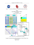
NASA
University of Oklahoma (OU) HyDROS Lab (http://hydro.ou.edu)
CREST
Coupled Routing and Excess STorage
User Manual
Version 2.1
(f)
(g)
By Dr. Xinyi Shen and Dr. Yang Hong
University of Oklahoma, National Weather Center, Norman, OK USA
Oct. 13, 2014
Cover: CREST—Coupled Routing and Excess Storage User Manual Version 2.1
Table of Contents
CREST ................................................................................................................ 1
TABLE OF CONTENTS ...................................................................................... I
1 MODEL OVERVIEW ...................................................................................... 2
1.1 Overview of CREST ............................................................................................ 2
1.2 What’s new in CREST v2.1 ................................................................................. 3
2 INSTALLATION .............................................................................................. 4
3 FRAMEWORK AND USER INTERFACE OF CREST V2.1 ........................... 5
3.1 Model Structure and running commands ......................................................... 5
3.2 Control File ........................................................................................................ 6
3.3 Folders and Files.............................................................................................. 15
4 RUN STYLES AND MODES ...........................................................................20
4.1 Outputs in the Simulation Style ...................................................................... 21
4.2 Outputs in the Calibration Style ...................................................................... 22
4.3 Flood Event (FE) Mode .................................................................................... 22
5 SETTING UP CREST IN OTHER BASINS ....................................................22
6 CONTACT US .................................................................................................23
7 SELECTED CREST MODEL RELATED REFERENCES .............................24
7.1 Model References ........................................................................................... 24
7.2 Additional References ..................................................................................... 24
I
1 Model Overview
1.1 Overview of CREST
The Coupled Routing and Excess STorage (CREST) distributed hydrological
model is a hybrid modeling strategy developed by the University of Oklahoma
(http://hydro.ou.edu) and NASA SERVIR Project Team (www.servir.net). The CREST
model was initially developed to provide real-time regional and global hydrological
prediction by running at fine spatiotemporal resolution with maintaining economical
computational cost (http://eos.ou.edu). CREST simulates the spatiotemporal variation
of water and energy fluxes and storages on
distributed grid cells of arbitrary user-
defined resolution, which enables multi-scale applications (Figure 1-1). The scalability
of CREST simulations is accomplished through the sub-grid scale representation of soil
moisture storage capacity (using a variable infiltration curve), multi-scale runoff
generation processes (using multi-linear reservoirs) and a fully distributed routing
scheme (using the fully distributed linear reservoir routing (FDLRR)). The primary
water fluxes such as infiltration and routing are physically affected by the geographic
variables land surface characteristics (i.e., vegetation, soil type, and etc.). The runoff
generation and routing components are coupled, therefore CREST includes more
realistic interactions between lower atmospheric boundary layers, terrestrial surface,
and subsurface water than other distributed hydrological models. The above features
make CREST applicable at global, regional, and catchment scales.
This user manual and the accompanying example basin provide a single basin helps
user to install, test and learn how to use the model. The CREST model is forced by
gridded potential evapotranspiration (PET) and precipitation datasets that are measured,
estimated or forecasted.
Users can freely switch between the simulation and
calibration running styles and between the continuous and flood events running modes
by simply modifying the control file.
2
Figure 1-1 Core Components of the CREST model
(a) Vertical profile of a cell including rainfall-runoff generation, evapotranspiration, sub-grid cell routing
and feedbacks from routing; (b) variable infiltration curve of a cell; (c) plane view of cells and flow
directions; and (d) vertical profile along several cells including sub-grid cell routing, downstream routing,
and subsurface runoff redistribution from a cell to its downstream cells.
1.2 What’s new in CREST v2.1
The major upgrade is on the routing scheme. The cell-to-cell routing scheme used
in previous versions of CREST is a quasi-distributed linear reservoir routing (QDLRR)
method which we found problematic to apply to a distributed hydrological model in
practice. In CREST v2.1, a fully distributed LRR method (FDLRR) is proposed and
used to replace the QDLRR module of CREST. The conception of the QDLRR and the
FDLRR is shown in Figure 1-2. Suppose that in one time step, water moves from A to
3
D, B to E and C to F and take C as the observation cell. In previous versions as shown
in Figure 1-2(a), only the water from C to F contributes to the final runoff (discharge)
of C while water from A to D and B to F is denied of contribution as if the water jumps
over cell C. On the contrary, in CREST v2.1, all these three terms contributes to the
runoff of cell C because they either sets off from or passed via cell C.
(a)
(b)
Figure 1-2 Routing Conception of v2.0 and v2.1. (a) Linear reservoir routing (LRR) method used in
V2.0 and (b) Fully distributed linear reservoir (DLRR) used in v2.1.
Minor upgrade includes: 1) the full vectorization of the computation which boosts
the efficiency by nearly one order (no routines loop cell by cell in the new version); 2)
acceptance of more advanced geographic data formats 3) automatic decompression,
reprojection, resampling and clipping of the forcing data to accommodate data in
different formats, coordinate system and resolution; 4) adding a flood event mode and
5) switching on and off a) the feedback mechanism, b) the existence of interflow in
channels.
2 Installation
CREST v2.1 is written in Matlab that is OS (operating systems) independent.
However, it integrates the GDAL libraries to implements I/O (input/output)
functionality, which is OS dependent.
On Windows x64 OS
The installation of CREST includes only a few steps on Windows OS:
1) Download the CREST and Dependency files from our website
http://hydro.ou.edu/research/crest-demo/
2) Decompress the two zipped files and put all subfolders and files in the same
4
folder. Consequently, you should have 6 components in your arbitrary
program folder
Figure 2-1 All components included in CREST v2.1
3) Start your Matlab Enviroment and navigate to your program folder, run the
install.m by typing the following command in the matlab command window,
>>install
On Linux
The linux compatible version is coming soon.
3 Framework and User Interface of CREST v2.1
3.1 Model Structure and running commands
Figure 3-1. Project structure of CREST v2.1
The user interface of CREST v2.1 is remains similar as that of CREST v2.0.
5
Although the data files needed in CREST can be stored anywhere in principle, it is
recommended to store all the data and control files needed by the given basin in a single
project folder.
In CREST v2.1, the control file is named “*.Project”, which stores the running
options and physical locations of all other data files needed by CREST and is usually
put in the root of the project folder. Other data files, as shown in Figure 3-1, are
distributed in several folders of the project according to their categories. These folders
are specified in the control file including “basic”, “rains”, “PETs” “Param”,
“obs”,”calib” and “results”.
The control file and these folders will be described in the following subsections.
Setting up a basin is to create and fill these folders and the control file.
After a basin is setup, users can run CREST using the following matlab command
>> CREST(globalCtl, opt, gdalPath, nCore);
where
globalCtl is the full path of the control file.
opt=’mean’|’real’ refers to use the presumed mean height difference or the real one at
the outlet. The mean height difference is usually used because the clipped geographic
data contained in the basic folder usually lacks the information of the next downstream
cell of the basin outlet and it can also be a “sink” at the outlet cell.
gdalPath is the path where gdal_csharp.dll is stored. By default, it should be in the
subfolder ”.\ gdal_1110_dll” in the decompressed CREST folder.
nCore is the number of allowed parallel workers. It is only effective in the calibration
mode and can be ignored in the simulation mode.
3.2 Control File
The control file described in this subsection contains model settings and data
directories.
Note:
The statements in the control file should be listed in order in a keywords-value
manner as following:
Keyword
=
6
Value
The statement appearing on the same line should be tab-separated.
Comment should begin with a pound sign, #.
Keyword is not case sensitive.
Note 1. Keyword and value format
Keywords with * is new in CREST v2.1.
Model Area (obsolete)
CREST v2.1 accepts common geographic data formats that contain information of
coordinate systems and projections. Therefore the “Model Area” is removed.
3.2.1 Temporal
Settings
The description of keywords and values in the Section of Temporal Settings is given in
Table 3-1.
Figure 3-2 A sample of temporal settings section in the control file (regular mode)
7
Figure 3-3 Sample temporal settings in the control file (flood event mode)
Table 3-1 Temporal Settings in the control file
Keyword
Value
Description
(type)
TimeMark
TimeStep
The unit of time step.
“d” (day), “h” (hour),
“u” (minute).
integer Time interval (step) in TimeMark
d|h|u
The time format convention used by all temporal variables
in this section
e.g. “yyyymmddHH”
The start time of the simulation or calibration. Its format
StartDate
date
is defined by TimeFormat
NLoad*
integer The number of flood events. In regular mode, Nload=0 and
“StartDate”, “WarmupDate” and “EndDate” controls the
running period. In flood event mode, CREST only
simulate/calibrate the period during “NLoad” flood events an
while “StartDate”, “WarmupDate” and “EndDate” are
ineffective
The ending date time of warming up of the simulation. Its
WarmupDate
date
format is defined by “TimeFormat”
The end time ofthe simulation, its format is defined by
EndDate
date
“TimeFormat”.
WarmupDate_i integer The beginning date time to load state variables to run CREST
TimeFormat*
string
in the flood event mode.
8
EndDate_i
integer The End date time to load state variables to run CREST in the
flood event mode, where 0<i<=NLoad. Its format is defined
by “TimeFormat”.
3.2.2 Style
and Options
Users set the running style and model options in this section in the control file.
Figure 3-4 A sample of the Style and Options Section in the control file
Table 3-2 Style And Options Section in the control file
Keyword
Value
Default
Description
RunStyle
simu|ca
N/A
“simu” stands for the simulation mode
lib_SC
while “calib_SCEUA” stands for the
EUA
automatic calibration mode using the SCEUA method.
Feekback*
Yes|No
“Yes” means that the routing process feeds
Yes
back the rainfall-runoff process
hasRiverInterflow
Yes|No
“No” means that all interflow turns to
No
*
useLAI*
3.2.3 Model
surface flow in channels
Yes|No
“Yes” is reserved for later versions.
No
Directory
In this section in the control file, directory of all input and output data files is specified.
9
Figure 3-5 Sample Model Directory in the control file
As shown in Figure 3-5, CREST separates the input and output data into 9
categories: “Basic”, “Param”, “States”, “ICS”, “Rains”, “PETs”, “Result”, “Calib” and
“OBS”. Each category has a standalone folder denoted by “*Path”, for example, the
“BasicPath”. The name of the folders is user-specified while the keywords are fixed.
The statements in this section is written in the keyword/value format defined in Note 1.
3.2.3.1 The Basic Section
The basic folder contains the raster files of the same format that stores the
geographic information of the basin. The full path of these files is “known” by
CREST using the information specified in this section as described in Table 3-3. For
e.g., the full path of the DEM file is specified as BasicPath +”dem”+ BasicFormat.
Table 3-3 Basic section in the control file
Keyword
Value
Description
BasicFormat
The extension of an image file.
Default is Geotiff ‘.tif’
file name extension
BasicPath
A string of a valid directory
that ends with a ‘\’
Physical path of the basic
folder
10
3.2.3.2 Param, State and ICS Sections
The “Param” and “ICS” folders contain text files of model parameters and the
initial condition respectively. The key/value format of these files appears the same as
in the control file defined in Note 1. The file format in “Param” and “ICS” folders is
fixed to ‘.txt’ while the format in the States folder is fixed to “.mat”.
3.2.3.3 Forcing Sections
The forcing Sections are the trickiest. It includes the rainfall, PET and the LAI
subsections. The three forcing sections have the same structure with the rainfall section
being shown in Figure 3-5 as an example. CREST incorporates two mechanisms to
efficiently read the forcing file: reading from external formats and from the internal
format. The external format can be in arbitrary image format of a standard coordinate
system. The internal format is in matlab’s “.mat” matrix. When the model runs in the
simulation mode, it first check the existence of internal files, if they exist, the model
uses read the internal files; otherwise, it tries to read the external file on the missing
date time and then save it in the internal format for next time use. Reading the external
forcing file can be significantly slower than the internal one because it may involve the
decompression, resampling, reprojection and clipping. As a result, it is recommended
to run the model in the simulation mode for the first time and then to play the model at
any styles the user desire.
Table 3-4 lists the variables in the rainfall section as an example. In this example,
daily stageIV data is used, the file name without directory is “yyyymmdd12.24h.Z”.
Table 3-4 Basic section in the control file
Keyword
Example Value
Description
RainFormat
.24h.Z
The extension of the EXTERNAL forcing
file. Note that the extension means all
content after the date time part
The file can be a compressed file. CREST
will identify this by its extension
(.zip, .rar, .z, .7z) and decompress it using
the user specified decompression
software if necessary. WinRAR is
currently
supported
in
windows
platforms.
RainDateFormat
yyyymmddHH
The time format used by RainStart, and
RainDateInterval.
RainDateConv
Begin|Center|End
The time convention used by the time
label (file name) of rain forcing files
RainStart
2002010112
The first start date time of
11
rain
forcing that will be used by the
model.
RainDateInterval
0000000100
The rain time interval in RainDateFormat.
RainPathExt
"\\server\StageIV_daily\ST4.”
The directory of external rain files
RainTsScaling
1
The scaling factor to convert the original
data contained in rain file to
mm/TimeMark.
RainPathInt
"\\Server\Tar\rains_daily\rain."
The directory of internal rain files.
3.2.3.4 The Result Section
The result Section specifies the directory of the result folder
3.2.3.5 The Calibration Section
The calibration Section specifies the directory of the calibration folder.
3.2.3.6 The Observation Section
The observation section
OutPix Information (obsolete)
Instead of outputting selected pixel information, CREST v2.1 outputs the selected
variables of the entire river network whose location is read from the stream file in the
basic folder.
3.2.4
Outlet Information
CREST v2.1 uses a point feature in the ESRI shape file format to represent the
location of the outlet rather than texts of the latitude and longitude. Therefore, only the
file name of the shape file is specified in the control file. In addition, the shape file
MUST contain a projection.
12
Figure 3-6 A sample of the outlet information in the control file.
Table 3-5 Outlet Information section in the control file
Keyword
Example Value
Description
HasOutlet
Yes|No
Yes: the basin has an outlet. In this version, it is always
yes.
OutletName
02083500
The name used to specify the observation file and the
first field of the site (a point feature) in the shape file.
OutletShpFile
02083500.shp
File name of the shape file that contains the outlet
location as a point feature. The first field of the point
feature must be the OutletName. The default directory
of the shape file is the “obs” folder.
3.2.5 Grid
Outputs
Grid Outputs is used to select the 2-D gridded variables to output at EVERY time
step. The selected (of Yes value) variables will be output to the result folder and the file
name will be suffixed by the date time in model’s temporal format. The default format
of the 2-D gridded files is GeoTiff (.tif). Grid outputs is time consuming and not
recommended during the calibration.
Figure 3-7 Sample Grid Outputs in the control file
Keyword
Description
GOVar_Rain
The input precipitation in mm/timestep
GOVar_PET
The input PET; in mm/timestep
GOVar_EPOT
GoVar_PET*KE, calibrated PET used in the model
13
GOVar_EAct
The actual evapotranspiration in mm/ timestep
GOVar_W
The depth of water filling the pore space bucket "WM"
GOVar_SM
volumetric soil moisture that equals GOVar_W/WM
GOVar_R
The simulated discharge of EACH grid cell IN THE RIVER in
m³/s.
GOVar_ExcS
The depth of surface excess rain in mm
GOVar_ExcI
The depth of infiltrated excess rain in mm
GOVar_RS
The depth of overland flow in mm
GOVar_RI
The depth of interflow flow in mm
3.2.6 State
to Save
CREST v2.1 is able to run at a flood event (FE) mode, in which the initial state of each event
must be reloaded. These states were saved during a previous simulation. The previous run can be at
a different time step while save the states as at an offset time (in its file name) to adjust to the time
line in the FE mode. For instance, in Figure 3-8, the first save date time is at 0:00 am., Oct. 8th,
2002. To adjust to a FE mode at hourly scale that centered at XX:30, a minimum 30 min offset is
added to make the first saving date time 00:30 am., Oct. 8th 2002.
Figure 3-8 Sample Output Dates in the control file
Keyword
Example Value
Description
NumOfOutputDates
24
The number of saving states
14
SaveDateFormat
OutputDate_i
“yyyymmddHHMM”
The date time format AFTER offset
2002100800
A string that contains the saving date time
BEFORE offset
3.3 Folders and Files
CREST v2.1 can read more than 200 the raster file formats supported by GDAL.
Users only need to prepare the basic files and other text files. The decompression,
reprojection, resample and clipping of the forcing file according to the configuration of
the basic file is automatically conduct by CREST. Therefore, Users can save their space
and time in preparing forcing files for each basin.
3.3.1 Basic
Folder
This folder contains the raster files that represent the geographic information of the
basin and a text file that defines the average height difference: a DEM (Digital elevation
model) file, an FDR (Flow Direction) file an FAC (Flow Accumulation) file a stream
file. All files except the slope file is in a geographic data format with a projection. From
CREST v2.1, the model accepts any commonly used raster formats supported by GDAL.
Raster files in this folder only contains grid-cell values within the basin area while the
grids out of the basin is marked by Null value which is explicitly recorded in the each
raster file, as done by the SetNull function of the ArcGIS Map Algebra tool. In addition,
the regions in all four raster files MUST have exactly the same size and basin area.
Users can use a GIS tool to generate the files in this folder. We also attached a python
script that calls ArcGIS routines to prepare all raster files for CREST.
Table 3-6 Contents in the basic folder
Name
Optional
Description
DEM
FDR
File name Format
by default
dem.*
any
fdr.*
any
No
No
FAC
fac.*
any
No
stream
slope
stream.*
Slope.def
any
.def (text)
No
No
The digital elevation model
Flow direction (code defined as in
ArcGIS, 1-128)
Flow accumulation (value defined as
in HydroSHEDS, i.e., the high
ends(minimum value) is 1) in pixel
Value in the river is 1, otherwise is 0
Contains the GM value that defines
the pre-defined mean height
difference. It is used for calculate the
slope at the outlet or other places
where the slope value is invalid from
15
the DEM map.
A second value is the height of the
adjacent downstream cell of the
outlet. The second value is optional.
Mask, GridArea and AreaFact files are obsolete since CREST v2.1.
3.3.2 Param
Folder
This folder contains a parameter.txt file that records all 15 model parameters that
are categorized as physical and conceptual types (see Table 3-7). The model parameters
in CREST v2.1.0 remains the same as in CREST v2.0.
The parameter.txt file also
Table 3-7 Classification in CREST v2.1
Type
Physical
Parameter
RainFact
Ksat
WM
B
Parameters
Conceptual
Parameters
IM
KE
coeM
expM
coeR
coeS
KS
KI
Min Default
Description
0.5
1.0
The multiplier on the precipitation field
0
500
The Soil saturate hydraulic conductivity
80
120
The Mean Water Capacity
The exponent of the variable infiltration
0.05
0.25
curve
0
0.05
The impervious area ratio
0.1
0.95
The factor to convert the PET to local actual
1
90
The overland runoff velocity coefficient
0.1
0.5
The overland flow speed exponent
1
2
The multiplier used to convert overland flow
The speed to channel flow speed
0.3
The multiplier used to convert overland flow 0.001
The speed to interflow flow speed
0
0.6
The overland reservoir Discharge Parameter
0
0.25
The interflow Reservoir Discharge Parameter
follows the keyword/value format defined in Note 2. Furthermore, each variable is not
only defined by its value, but also defined by its type, i.e., the “varNameType”
keyword. The type can only be uniform or distributed. If the type of a parameter is
distributed, it’s the value should be a file name in the “Param” folder of a raster file
that exactly matches size and basin area defined by the files in the basic folder. The
limits and the default value of uniform parameters are also listed in Table 3-7.
16
Max
1.2
3000
200
1.5
0.2
1.5
150
2
3
1
1
1
3.3.3 State
Folder
This folder contains the saved model state files named by the date time specified in
Section 3.2.6. The state files are in matlab “.mat” format. The State folder is an output
folder for regular running mode whereas an input folder for the FE mode. In the FE
mode, CREST loads the state variables saved by a previous simulation in the regular
mode. However, the date time to load is specified in the “temporal Settings” section in
the control file rather than the “State to Save” section.
3.3.4 ICS
Folder
This folder has an “initilalCondition.txt” file that contains uniform variables listed in
Table 3-8 as the model initial condition. The initial condition file is written in the same
format as the parameter file. To let CREST be well distributed, a sufficient warm up
period is necessary. This folder is ineffective in the FE mode.
Table 3-8 Classification in CREST v2.1
Keywords
W0
SS0
SI0
Unit
%
mm
mm
Description
Initial Value of Soil Moisture
Initial value of Overland Reservoir
Initial value of Interflow reservoir
Default values of these variables are in Table 3-7.
3.3.5 OBS
Folder
This folder contains the shape file (location) of the outlet and the observed runoff
data excel file.
for the model calibration or validation. The file name of the observed
runoff is “OutletName_Obs.csv” (“.csv” is the comma delimited file) where the
“OutletName” is specified in the project file and the file name of the shape file is
specified in the control file. The OutletName_Obs.csv has two columns WITH head.
The first and second columns record the date time and runoff respectively. The date
time must follow the
It should be noted that the shape file contains the outlet position as a point feature.
17
The value of the first field of the point feature must be the OutletName.
3.3.6 Calibs
Folder
This folder has a “calibration.txt” file that contains the calibration configuration
site name and ratio limits of the model parameters as shown in Figure 3-8 and detailed
in Table 3-9.
Figure 3-9 Sample of “Calibrations.txt” file
Table 3-9 content in the Calibrations.txt
keyword
iseed
Type
SCE_UA
maxn
SCE_UA
kstop
SCE_UA
pcento
SCE_UA
Description
The initial random seed
The max no. of trials allowed before
optimization is terminated
The mumber of shuffling loops in which
the criterion value must change by the
given percentage before optimization is
terminated
The Percentage by which the criterion
value must change in given number of
shuffling loops
ngs
SCE_UA
The Number of complexes in the initial
population
18
NCalibStations
Stations
Name_i
Stations
The Number of Calibrated Stations
The name of the ith station
Rainfact_i
parameters
The possible range of RainFact
...
parameters
…
The format of for parameters to be calibrated is:
ParameterName_i
=
Min
Value
Max
where, i is the station No. and Min, Value, Max are the lower limit, initial value and up
limit of the parameter to be calibrated. This file is only required in the calibration style.
Note that the limits and value of all parameters in the calibration.txt are ratios rather
than absolute values. The actual value of a given parameter in the model is the product
of its ratio in the “calibration.txt” and its value in “parameters.txt” in a calibration
running style. In the simulation style, the calibration folder is ineffective. Currently,
CREST only supports single site calibration. Therefore, NCalibStations≡1 and i≡1.
Multi-site calibration mode is coming soon.
3.3.7 PETs
Folder
This folder only contains the INTERNAL potential evaporation data files named by
their date time. Please refer to Chapter 3.2.3.3 on the data time format and directory of
this folder. And. In the first time simulation of the basin, if the PETs empty, CREST
v2.1 automatically decompresses (if necessary), re-project, resample and clip the
external forcing file to the projection, region and resolution defined in your basic
(geographic) files. The processed forcing files will be saved in internal “.mat” format
in this folder. For later runs, if CREST finds the internal forcing files, it will ignore the
external ones and use the internal ones directly. In practice, we encourage you to store
your global/regional external forcing files in one fixed location and let model convert
between the external and internal files to save your space and preprocessing time. Due
to the complex procedure of importing external files, it can be time consuming in
simulating a basin for the first time. However, for later simulations or calibrations, the
model runs significantly faster.
19
3.3.8 rains
Folder
This folder only contains the internal rainfall files named by their date time. Please
refer to Chapter 3.2.3.3 on the data time format and directory of this folder.
All rules
in Chapter 3.3.7 apply in this folder as well.
3.3.9 Results
Folder
This folder contains hydrographs, output variables and calibration results in multiple
formats.
4 Run Styles and Modes
In this chapter, we introduce the output differences between running styles and
modes. Please refer to 3.2.2 on how to set different running styles and modes in the
control file. In CREST v2.1, there are the simulation and calibration running styles,
regular and flood event modes.
20
4.1 Outputs in the Simulation Style
…
Figure 4-1 Screen output in simulation style.
The hydrographs and other selected model output variables are stored the results
folder. The hydrograph is a excel file named by its corresponding outlet as shown in
Figure 4-2 . If some gridded outputs are enabled, image files named by the date time are
also generated in the result folder.
21
Figure 4-2 snapshot of the hydrograph file.
4.2 Outputs in the Calibration Style
Since CREST v2.0, SCE-UA (Duan et al., 1992) is selected as the kernel algorithm
in calibration process. In CREST v2.1, SCE-UA is parallelized using the shared
memory multiprocessing (OpenMP) approach.
CREST v2.1 directly uses the screen output of SCE-UA codes in matlab written by Duan et al.,
1992. The objective function value is the NSCE of each simulation. CREST v2.1 also outputs
the calibration process to a log file in the “Results” folder, named as “log.txt”. The
calibration result
is output both to the screen and
to a
file named
“SCE_UAyyyymmdd_hh.txt” in the same folder.
4.3 Flood Event (FE) Mode
The only difference between the FE and regular mode is that the FE mode only outputs
everything within the period of the flood events specified in the control file. The FE mode can be
used in both simulation and calibration style and saves a lot of computational time since it skips the
non-flood event periods. Please refer to Section 3.2.1 about the FE mode.
5 Setting up CREST in other basins
Users can run CREST in their own basins after installation. The CREST model
automatically runs over the region defined by geographic images in the basic folder. All
files in this folder must be prepared before running the models. Forcing files are also
necessary but CREST deals with most of the preprocessing.
Please follow the steps below to setup a basin of a user’s own.
1. Create a project folder that contains all folders described in Chapter 3.3.
22
The name of the project folder is arbitrary.
2. Create a control file by either
a. Copying the existing project file provided in the example Tar basin
folder and modifying the content according to your own basin.
or
b. Filling the content following the instructions in Chapter 3.2.
Please note that all sections in the control file are necessary for CREST.
Please use the switchers to mute the sections not needed rather than
removing those sections
3. Generate the geographic (basic) files required in the basic. Please also refer
to Chapter 3.3.1 for the definition and generation of basic files.
4. Create and fill the files needed in the “Param” and “ICS” folders. Please
refer to Chapters 3.3.2 and 3.3.4
for the files in these folders.
5. Prepare the observation files needed in the “OBS” folder. Please refer to
Chapter 3.2.3.6 and 3.3.5 for these files.
6. Run the model in simulation style using the commands introduced in
Chapter 3.1.
7. If a calibration process is needed, please also create and fill the files in the
“Calibs” folder and switch the running style in the control file accordingly.
Please refer to Chapter 3.3.6 for the calibration file and the parameter
difference in the calibration and simulation styles. The parameters used in
the simulation style and calibration style are determined by different files.
Note that a lot of users failed to calibrate the model by failing to notice this
difference.
8. A user must remember to multiply the calibrated “ratios” and magnitude
values in the parameter file used in the calibration process provided he
needs to simulate the basin using his calibrated model parameters.
6 Contact us
The official version of the OU-NASA CREST model has been developing and
23
maintaining in the Hydrometeorology and Remote Sensing Laboratory, University of
Oklahoma (http://hydro.ou.edu) and Atmospheric Radar Research Center (ARRC)
located in the National Weather Center (http://nwc.ou.edu). For the information about
the current release of the CREST model, the source code of beta versions and technical
support, please send e-mail to Prof. Yang Hong ([email protected]) and Dr. Xinyi Shen
([email protected]).
7 Selected CREST model Related References
7.1 Model References
Xinyi Shen, Yang Hong, Ke Zhang and Zengchao Hao, (2014). “Refine a Distributed
Linear Reservoir Routing Method to Improve Performance of the CREST
Model” (submitted).
Wang. J., Y. Hong, L. Li, J.J. Gourley, K. Yilmaz, S. I. Khan, F.S. Policelli, R.F. Adler,
S. Habib, D. Irwn, S.A. Limaye, T. Korme, and L. Okello, (2011). “The Coupled
Routing and Excess STorage (CREST) distributed hydrological model”. Hydrol.
Sciences Journal, 56, 84-98.
7.2 Additional References
Xue X, Hong Y, Limaye AS, Gourley JJ, Huffman GJ, Khan SI, et al., 2013: Statistical
and hydrological evaluation of TRMM-based Multi-satellite Precipitation
Analysis over the Wangchu Basin of Bhutan: Are the latest satellite precipitation
products 3B42V7 ready for use in ungauged basins? Journal of Hydrology,
499(0): 91-99.
Khan, S. I., Y. Hong, J. Wang, K.K. Yilmaz, J.J. Gourley, R.F. Adler, G.R. Brakenridge,
F. Policelli, S. Habib, and D. Irwin, 2011: Satellite Remote Sensing and
Hydrologic Modeling for Flood Inundation Mapping in Lake Victoria Basin:
Implications for Hydrologic Prediction in Ungauged Basins, IEEE Transactions
on Geosciences and Remote Sensing, 49(1), 85-95, Jan. 2011, doi:
24
10.1109/TGRS.2010.2057513
Wu H, Adler RF, Hong Y, Tian Y, Policelli F., 2012: Evaluation of Global Flood
Detection Using Satellite-Based Rainfall and a Hydrologic Model. Journal of
Hydrometeorolog, 13(4): 1268-1284.
Duan, Q., Sorooshian, S., Gupta, V., 1992. Effective and efficient global optimization
for conceptual rainfall‐runoff models. Water Resour. Res., 28(4): 1015-1031.
25