Download A Model Checking Approach to Protocol Conversion

A Model Checking Approach
to Protocol Conversion
Technical Report
No.0000482
Roopak Sinha, Partha Roop
Department of Electrical and Computer Engineering
University of Auckland
and
Samik Basu
Department of Computer Science
Iowa State University
Iowa State University
Department of Computer Science
November, 2006
c
2006
All rights reserved
Abstract
Protocol conversion for mismatched protocols has been addressed in
a number of formal and informal settings. However, existing solutions
address this problem only partially. This paper develops the first on-thefly local approach to protocol conversion based on temporal logic model
checking. The tableau-based approach verifies the existence of a converter,
and if a converter exists, it is automatically synthesized. Our approach
handles control and data mismatches under a single unifying framework.
A NuSMV-based implementation has been developed and we provide results
for some non-trivial protocol mismatch examples.
1
Introduction
A system-on-a-chip (SoC) is built by reusing components connected using a
central bus such as AMBA [3]. A major problem with this reuse is the inherent mismatch between protocols of components, an active area of research for
about two decades [7]. Mismatches occur because components are developed
independently without any intention of eventual integration, and can result
from control signal mismatches [6], inconsistent naming conventions [11], different clock speeds and difference in data-widths [3]. Mismatches are corrected,
if possible, by synthesizing extra glue-logic, called a converter [10] to control
communication between given protocols in order to satisfy given specifications.
A number of techniques address the problem of protocol conversion in a wide
range of formal and informal settings with varying degrees of automation—
projection approach [7], conversion seeds [9] and synchronization [11]. Some
approaches, like conversion seeds [9] and protocol projections [7], require significant user expertise and guidance. While this problem has been studied in a
number of formal settings [6, 7, 9, 11], only recently have some formal verification based solutions been proposed [3, 5, 10].
In [5], a hybrid simulation/verification approach to protocol conversion in
SoC designs is proposed. [10] proposes an approach towards protocol conversion
employing a game-theoretic framework to generate a converter. This solution is
restricted only to protocols with half-duplex communication between them, with
specifications represented as finite state machines. D’Silva et al [3] present synchronous protocol automata to allow formal protocol specification and matching,
as well as converter synthesis. The technique addresses the problem of limited
communication medium capacity, but data-communication between protocols
cannot be constrained any further.
P1
Converter
P2
Specifications
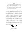
Figure 1: Protocol conversion
1
In contrast to the above techniques, we present a technique using model
checking for automatic converter synthesis. Protocols, in our setting, are represented using Kripke Structures (KS) and specifications (and their negations)
are expressed in the temporal logic ACTL. ACTL, a branching time temporal logic
with universal path quantifiers, is particularly relevant for protocol conversion
as mismatches in protocols must be addressed for every path of their KS descriptions. Given two KSs P1 and P2 and a set Ψ of desired ACTL properties,
the protocol conversion via converter synthesis problem (illustrated in Fig. 1)
may be stated as:
Can a converter C be synthesized for P1 and P2 such that all formulas in Ψ can be satisfied?
The proposed approach involves the local and on-the-fly construction of a
tableau [2] where satisfaction of ACTL formulas in Ψ is defined in terms of the
satisfaction of their subformulas by the states of the protocols. The tableau
construction results in the automatic synthesis of the converter, if one exists. If
no converter is found, failures can be identified without exploring states irrelevant for failure inference. Not only are temporal logic specifications succinct
and more intuitive to write, additional constraints such as fairness can also be
specified. Fairness constraints ensure that converters allow meaningful communication to take place between protocols. We use invariants to specify bounds
on data-widths [1] so that data-width mismatches are addressed.
The main contributions of this paper are:
• We propose the first model checking based solution to protocol matching guaranteed to produce a converter if one exists—no further proof of
correctness is required, unlike some other approaches [3].
• We present a novel tableau-based algorithm to address data and control
mismatches in a unifying manner, unlike earlier solutions that deal with
them separately or in an ad hoc manner.
• We present an on-the-fly algorithm for converter synthesis, one where protocol states are explored only when needed. The algorithm is polynomial
in the size of the protocols and specifications.
The rest of this paper is organized as follows. Section 2 presents the automatic converter synthesis approach based on tableau generation. Section 3
provides some implementation results with concluding remarks in section 4.
2
Methodology
The proposed protocol conversion algorithm takes as input the KS descriptions
of two protocols and a set of ACTL properties. It then employs a local, on-thefly tableau construction algorithm to verify the existence of a converter.
2
<2>
<2>
s0
T
Idle
T
T
<1>
s1
R_Out
s3
<1>
ack
<2>
s2
Error
more
Req_In
T
<2>
Producer
<1>
req
t1
D_Out
8
<1>
T
T
<1>
<2>
req
t0
Idle
T
t3
t2
ack
Ak_Out
<1>
<1>
D_In16
d_rdy
T
<2>
Consumer
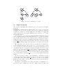
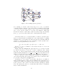
Figure 2: Producer-consumer protocol pair
2.1
Input description
The conversion algorithm takes as input two protocols represented as Kripke
structures:
Definition 1: A Kripke structure (KS) is a finite state machine represented as
a sextuple AP , S, s0 , Σ, R, L, where AP is a set of atomic propositions; S
is a finite set of states; s0 ∈ S is the initial state; Σ is a finite set of input and
output events; R ⊆ S × Σ × S is the transition relation; and L : S → 2AP is the
state labelling function.
States in a protocol are labelled by unique identifiers. Transitions between
states, each labelled with a priority, trigger with respect to a clock. At each clock
cycle, the KS checks for the presence of input/output events that can trigger a
transition from the current state. If multiple input/output triggers are present,
the transition using the highest priority is taken. An event a represents an input
whereas a represents an output. The relations (s, a, s ) ∈ R are represented as
a
s → s .
Fig. 2 shows the protocols of two devices, a producer and a consumer represented as Kripke structures. The producer protocol P1 , sends sends a request
before producing any data and in the next cycle awaits the input signal ack. If
ack is absent, the protocol enters an error state (s2 ). Else, it goes on to write
8-bits on to the data channel D out8 and is capable of writing multiple 8-bit
data if the signal more is present in subsequent cycles. The 16-bit consumer,
P2 , reads the request from the producer and then emits an acknowledgement
(ack). It then waits for the input d rdy to read one 16-bit data from the data
channel.
The protocols have a number of incompatibilities. Although P1 and P2
can share the input/output channels req and ack, but there are no outputs
corresponding to the control inputs d rdy and more (control incompatibility).
Furthermore, there is also a data incompatibility as P1 writes 8-bit data whereas
P2 can only read 16-bit data.
In addition to addressing the above issues, the intended communication between the producer-consumer protocols can be further described using addi-
3
tional ACTL formulas. ACTL is a fragment of the branching time temporal logic
CTL and only allows universal path quantifiers. Semantics of an ACTL formula, ϕ
denoted by [[ϕ]]M are given in terms of set of states in a KS, M , which satisfies
the formula. A state s ∈ S is said to satisfy a ACTL formula ϕ, denoted by
s |= ϕ, if s ∈ [[ϕ]]M . We also say that M |= ϕ to indicate that the initial state s0
of the model M satisfies ϕ. We restrict ourselves to formulas where negations
are applied to propositions only. For the producer-consumer example in Fig. 2,
the following properties are needed:
1. A(¬Req In U R Out) (S1): A request cannot be read before one is made.
2. A(¬D Out8 U Req In) (S2): No data is written data before a request has
been received.
3. AG(¬Error) (S3): The communication never enters a state labelled by
Error.
2.1.1
Describing data-width mismatches
The producer-consumer protocol pair has a data-width mismatch as P1 writes
8-bit numbers to the data channel whereas P2 reads 16-bit numbers. We formally describe the desired data-communication behaviour as follows. Given the
data-widths N and M of the outputs and inputs respectively, we first compute
the minimum width needed for the communication medium between the two
protocols. If N < M , then the minimum capacity must be N × f such that
f is the smallest integer for which N × f > M ; otherwise the minimum capacity is N . This ensures that there are enough preceding outputs before any
one input. While the minimum bound of communication medium buffer can
be computed as above, the maximum bound is be any value greater than the
minimum bound. In our setting, we assume that the maximum bound of the
communication medium buffer is LCM(N, M ). Given a capacity K of the communication medium between these bounds, the maximum number of outputs
possible when the medium is empty is x = K/N ; while the maximum number
of inputs possible when the medium is full is y = K/M . We use an auxiliary
counter for every input/output pair such that the counter is incremented by y
for every output, decremented by x for every input, and verify that the counter
always remains between 0 and x × y using the invariant 0 ≤ counter ≤ (x × y).
In addition, we can also force that maximum number of outputs are done
before inputs start and vice versa—expressed by the following ACTL formulas:
AG(counter = 0 ⇒ A(¬input U counter = x × y) )
AG(counter = x × y ⇒ A(¬output U counter = 0) )
For the producer-consumer example in Fig. 2, we use the invariant 0 ≤
counter ≤ 2 as N =1 and M =2.
4
Node
s (state)
labels (set of formulas)
type (either OR or AX)
counters
Node
Leaf
s (state)
labels (set of formulas)
type (either AND or OR)
counters
s (state)
F (set of formulas)
counters
Figure 3: The structure of nodes and leaves
2.1.2
Fairness
In order to ensure that converters always allow meaningful communication between protocols, it may be desirable that additional fairness conditions are satisfied, which can be again defined using ACTL formulas. For converter synthesis,
the goal is to ignore as well as disable all unfair behaviours of the protocols. For
the producer-consumer example, we use the following fairness conditions:
• AGAF(D Out8 ) (F 1): The producer can always eventually write data.
• AG(D Out8 ⇒ AXA(¬Req Out U Data In16 ) (F 2): Once some data is written, no further requests are allowed before a read operation is performed.
• AGAF(R Out) (F 3): The producer can always eventually emit requests.
2.2
Tableau Construction Algorithm
The proposed technique is based on model checking and involves on-the-fly
tableau construction, similar to [2]. Given the inputs P1 and P2 describing
participating protocols, some invariants over data counters, and the set Ψ of
desired properties (including fairness properties), the tableau construction algorithm proceeds as follows. We illustrate the working of the tableau construction
algorithm using the producer-consumer example given in Fig. 2.
The first step is the computation of the unrestricted combined behaviour
P1 ||P2 of P1 and P2 , also called the parallel composition (similar to the synchronous parallel in Argos [8]), defined as follows.
Definition 2: Parallel Composition.
Given two Kripke structures P1 = AP1 , S1 , s01 , Σ1 , R1 , L1 and P2 =
AP2 , S2 , s02 , Σ2 , R2 , L2 , , their parallel composition, denoted by P1 ||P2 is
5
Node 1
0,0
Idle
req,T
T,req req,req
T,T
0,1
0,0
1,1
Idle
Req_In
Idle
T,T
2,2
Error
Req_In
T,T
0,2
Idle
Ak_Out
R_Out
Req_In
Error
Ak_Out
3,1
D_Out8
Ak_Out
Node 3
T,T
D_Out8
Req_In
T,d_rdy
0,3
D_Out8
Ak_Out
3,3
Idle
D_In16
Node 4
D_Out8
D_In16
0,1
c=0
F = {S1,S2,S3,F1,F2,F3,A(tt
U R_Out), A(tt U D_Out8)}
Leaf 2
T,ack
2,2
c=0
F = {S3,F1,F2,F3,A(tt U
R_Out), AXA(tt U D_Out8)}
Leaf 3
ack,ack
more,T
0,3
c=-1
F = {S3,F1,F2,F3,A(tt U
R_Out), AXA(tt U D_Out8),
A(~Req_Out U Data_In16)}
3
ack,ack
T,T
7
more,d_rdy
more,d_rdy
3,3 type = AX c=0
labels = {AX(S3), AX(F1),AX(F2),
AX(F3), AXA(tt U R_Out)}
(a)
0
req,req
req,req
3,2 type = AX c=1
labels = {AX(S3), AX(F1),AX(F2),
AX(F3), AXA(tt U R_Out),
AXA(~Req_Out U Data_In16)}
more,d_rdy
more,T
T,req
1,1 type = AX c=0
labels = {AX(S3),
AX(F1),AX(F2), AX(F3),
AXA(tt U D_Out8)}
R_Out
Idle
ack,T
3,2
3,2
Node 2
1,0
ack,ack
T,ack
2,1
Leaf 1
0,0 type = AX c=0
labels = {AX(S1),AX(S2), AX(S3),
AX(F1),AX(F2), AX(F3), AXA(tt U
R_Out), AXA(tt U D_Out8)}
10
(b)
(c)
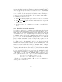
Figure 4: Tableau construction procedure. (a) states of P1 ||P2 , (b) tableau
nodes, (c) synthesized converter.
AP1||2 , S1||2 , s01||2 , Σ1||2 , R1||2 , L1||2 where AP1||2 = AP1 ∪AP2 ; S1||2 = S1 ×S2 ;
s01||2 = (s01 , s02 ); and Σ1||2 ⊆ Σ1 × Σ2 . R1||2 ⊆ S1||2 × Σ1||2 × S1||2 such that
σ
σ
(s1 →1 s1 ) ∧ (s2 →2 s2 ) ⇒ ((s1 , s2 )
(σ1 ,σ2 )
→
(s1 , s2 ))
Finally, L1||2 ((s1 , s2 )) = L1 (s1 ) ∪ L2 (s2 ).
Some states of the parallel composition of the producer-consumer example
are shown in Fig. 4(a).
Algorithm 1 check(s0 , Ψ)
1:
2:
3:
4:
5:
6:
7:
8:
9:
10:
11:
12:
13:
Initialize counters, create a set A of leaves.
call create leaf (s, counter vals, Ψ, Nil)
while A is non-empty do
remove one leaf t from A
result = solve leaf (t)
if result = SUCCESS or FAILURE then
result = notif y parent(t, result)
if globalresult = SUCCESS then
return SUCCESS
end if
end if
end while
return FAILURE
The proposed algorithm constructs a tableau which has nodes and leaves
(Fig. 3). Nodes are parents that have one or more children. Each node corresponds to a state in P1 ||P2 and a specific valuation of all data counters, and
is labelled with a set of formulas labels. Leaves, on the other hand, do not
6
have children, and have no labels. A leaf contains a set of formulas F that its
corresponding state must satisfy. The tableau can be extended only when a leaf
is expanded into a node.
Given the states of P1 ||P2 for the producer-consumer example (Fig. 4(a)),
the algorithm proceeds as follows. The initial state (s0 , s0 ) of P1 ||P2 and the
set Ψ ({S1, S2, S3, F 1, F 2, F 3}) are passed to the top-level tableau construction procedure check which initializes data counters and creates a set A, which
contains all leaves created during tableau construction. check then contains the
initial top-level tableau leaf corresponding to (s0 , s0 ) and the set of properties
Ψ. This is the root of the tableau which contains the initial state of P1 ||P2 and
the original set of properties Ψ. The method create leaf is used to create new
leaves. If the creation of a leaf results in the violation of any invariants, the
leaf is deemed invalid. After creating the root leaf, check calls the procedure
solve leaf for this newly created leaf.
Algorithm 2 create leaf (s, prevc ounterv als, Ψ, parent)
1: Update counters based on labels of s.
2: return if counters violate invariants.
3: if there exists a leaf t with t.state = s and t.counter status = current
counter status then
4:
t.f ormulas = t.f ormulas Ψ
5: else
6:
create a new leaf t with t.state = s
7:
t.f ormulas = Ψ, t.parent = parent, t.type = LEAF .
8:
t.counter status = updated counter status.
9: end if
The solve leaf method receives a tableau leaf t as input and proceeds to
individually break down formulas contained in t.F into current-state and future
commitments (lines 4-18). This decomposition of formulas is based on a set
of tableau rules (Fig. 5. For example, for root leaf of the producer-consumer
example, the formula S3 (AG(¬Error)) is broken down into the subformulas
Error and AXAG(¬Error). The sub-formula Error, being a current-state commitment (a proposition), is checked against the leaf state (s0 , s0 ). The future
commitment AXAG(¬Error) is stored in the set label. Once all current-state
commitments have been checked, the root leaf is expanded to become a node
(Node 1 in Fig. 4(b)) and a leaf is created for each successor of the state (s0 , s0 ).
All future commitments (including AXAG(¬Error)) are added to the set labels
of the newly expanded node, and (after removing AX from the formulas) to the
set F of each of the newly created leaves. Node 1 becomes an AX N ODE
as only those successors of the state t.state can be enabled that satisfy these
future commitments. Another case when a node may be expanded is when an
OR formula is encountered and the success of the parent node depends on the
success of any of its children. When a leaf is expanded (as in the case of the
root leaf for the producer-consumer example), the keyword EXP AN DED is
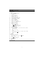
7
emp
−
(s,→
c )//c |={}
•
prop
−
(s,→
c //c |= [p ∪ Ψ]
s//c |= Ψ
→
(s,−
c )//c |= [ϕ ∧ϕ
−
p ∈ L(s) ∨ →
c |= p
∪ Ψ]
1
2
∧ (s,−
→
c )//c |= [{ϕ1 ,ϕ2 } ∪ Ψ]
→
(s,−
c )//c |= [ϕ ∨ϕ
→
(s,−
c )//c |= [ϕ ∨ϕ
∪ Ψ]
1
2
∨1 (s,−
→
c )//c |= [{ϕ1 } ∪ Ψ]
∪ Ψ]
1
2
∨2 (s,−
→
c )//c |= [{ϕ2 } ∪ Ψ]
→
(s,−
c )//c |= [A(ϕ U ψ) ∪ Ψ]
unrau (s,−
→
c )//c |= [(ψ∨(ϕ∧AXA(ϕ U ψ))) ∪ Ψ]
→
(s,−
c )//c |= [AGϕ ∪ Ψ]
unrag (s,−
→
c )//c |= [(ϕ∧AXAGϕ) ∪ Ψ]
→
(s,−
c )//c |= Ψ
unrs ∃π⊆Π. (∀σ∈π. (s ,−
→
σ cσ )//cσ |=ΨAX )
⎧
⎨
⎩
ΨAX = {ϕk | AXϕk ∈ Ψ}
σ
→
→
Π = {σ | (s, −
c ) → (s , −
c )}
σ
σ
σ
cσ = c : c → c ∧ D(σ, σ )
Figure 5: Tableau Rules for converter generation
returned by solve leaf .
For the producer-consumer example, root node 1 (Fig. 4(b)) has 4 children.
check iteratively calls solve leaf on all newly created leaves. When solve leaf
operates on leaf 1 (a child of node 1), it returns a F AILU RE. This happens
because the violation of the property S1. S1 is broken down to the currentstate commitment R Out ∨ (¬R In ∧ AXA(¬R In U R Out) which is not satisfied
by the state (s0 , s1 ) (the state corresponding to leaf 1). The check procedure
then passes the returned value to the method notif y parent, which effectively
results in the transition from (s0 , s0 ) to (s0 , s1 ) to be disabled in the tableau.
Another child leaf of node 1 corresponding to (s1 , s1 ) satisfies all its current-state
commitments and hence is further expanded into node 2 with 4 children. Its
child leaf 2, corresponding to the state (s2 , s2 ) in P1 ||P2 returns a F AILU RE
as it is labelled by Error (violates S3).
The child leaf corresponding to the state (s3 , s2 ) is expanded (node 3) with
only 3 children even though the state (s3 , s2 ) has 4 successors. This is so because
the child leaf 3 corresponding to the state (s0 , s3 ) is invalid as the data read
(D In16 ) in this state results in the counter c taking a value (-1) which is outside
the allowed invariant range (0 ≤ c ≤ 2).
One of the children of node 3, corresponding to the state (s3 , s3 ) is further
expanded into node 4 with 2 child leaves (one for each successor (s3 , s0 ) and
(s0 , s0 )). The leaf corresponding to (s3 , s0 ) returns F AILU RE (counter out
of bounds), whereas (s0 , s0 ) returns SU CCESS. This happens because all
formulas passed to this child leaf are contained in the labels of the ancestor
node 1 (corresponding to the same state (s0 , s0 ) and counter valuation (c = 0).
Due to this, solve leaf does not store any further future commitments (all of the
type AXAG (lines 24-33) and as all current-state commitments are met, returns
8
Algorithm 3 solve leaf (t)
1:
2:
3:
4:
5:
6:
7:
8:
9:
10:
11:
12:
13:
14:
15:
16:
17:
18:
19:
20:
21:
22:
23:
24:
25:
26:
27:
28:
29:
30:
31:
32:
33:
34:
35:
36:
37:
38:
39:
40:
41:
42:
43:
s = t.state, Ψ = t.F
Initialize ΨAX
while Ψ is non-empty do
remove one formula f from Ψ
if f = TRUE then
continue
else if f = FALSE then
return FAILURE
else if f = p ∈ AP then
return FAILURE if not f ∈ L(s)
else if f = ¬p (p ∈ AP ) then
return FAILURE if f ∈ L(s)
else if f = AGP then
insert P ∧ AXAGP in Ψ
else if f = A(P U Q) then
insert Q ∨ (P ∧ AXA(P U Q)) in Ψ
else if f = P ∧ Q then
insert P, Q in Ψ
else if f = P ∨ Q then
t.type = OR N ODE
S
S
create leaf (s, Ψ S{P } S ΨAX , t)
create leaf (s, Ψ {Q} ΨAX , t)
return EXPANDED
else if f = AXP then
if P = A(Q U R) and P occurs earlier in tableau at s then
return FAILURE
else
add f to the set ΨAX
end if
if P = AGQ and no ancestor of t contains P at state s then
add f to the set Ψ AX
end if
end if
end while
if ΨAX is non-empty then
ΨAX = {p|AXp ∈ ΨAX }, t.type = AX N ODE
t.labels = label
for each successor s’ of s do
create trace(s , ΨAX , t)
end for
return EXPANDED
end if
return SUCCESS
9
SU CCESS. This results in the tableau being folded back with a reference to
node 1. A similar leaf may return F AILU RE if the future commitments are of
the type AU.
The return values SU CCESS or F AILU RE returned by solve leaf for a
leaf t is passed to the notif y parent method which recursively passes the result
to its parent (ancestors if needed). A node returns SU CCESS if at least on of its
children returns SU CCESS. An OR N ODE does not disable any transitions
(as only one child is needed to satisfy commitments), whereas an AX N ODE
enables transitions to only those children that satisfy the future commitments
passed to them. The algorithm finishes when the root leaf (corresponding to
(s0 , s0 )) returns SU CCESS.
Algorithm 4 notif y parent(t, result)
1: if t is a top-level trace then
2:
globalresult = result
3:
return
4: end if
5: parent = t.parent
6: if parent.type = OR N ODE then
7:
if result = FAILURE then
8:
call notif y parent(parent, FAILURE) if no unchecked child remains.
9:
else
10:
call notif y parent(parent, SUCCESS)
11:
end if
12: else if parent.type = AX N ODE then
13:
if result = FAILURE then
14:
remove the link from parent to t.
15:
if child-set of parent is empty then
16:
call notif y parent(parent, FAILURE) if successor set of parent.state
is empty
17:
else call notif y parent(parent, SUCCESS)
18:
end if
19:
end if
20: end if
2.3
Converter Synthesis
The converter is synthesized automatically during tableau construction if it
completes successfully. We traverse the nodes (starting from the root node that
returned SU CCESS) in the tableau and select the AX nodes encountered to
form states in the converter. The converter states synthesized for the states of
P1 ||P2 for the producer-consumer example shown in Fig. 4(a), are shown in Fig.
4(c). Note how each converter state corresponds to an AX node in the tableau
(Fig. 4(b)). The full converter C is shown in Fig. 7.
10
The converter resolves incompatibilities between P1 and P2 as follows. The
input (output) events in P1 ||P2 are output (input) events for the converter. The
converter can read an output generated by either protocol and may pass it to
the other. Using this underlying control, the controller can perform inhibition,
buffering and synthesis. The converter inhibits an event when the transition
resulting from an event is disabled in C itself. In this case, the converter disallows
(or absorbs) the input instead of passing it on. The converter may buffer an
event, where it holds an input for a while before passing it on. Finally, in
case a control input expected by one protocol is not provided by the other,
the converter synthesizes it as an output itself in order to avoid blocking states.
The converter C (Fig. 7) for the producer-consumer example resolves the control
incompatibility between the two protocols by synthesizing the signals more and
d rdy artificially when required. The data incompatibility is resolved as all
paths leading to states where a mismatch happens (the counter variable in the
tableau exceeds invariant range) are disabled using inhibition. Furthermore,
buffering and inhibition are used such that only those paths that satisfy the
given ACT L specifications and fairness properties are also satisfied.
Formally, the control of a converter C over given protocols P1 and P2 , called
the lock-step composition C//(P1 ||P2 ), is defined as follows
Definition 3: Lock-step Converter Composition. Given the KS P1||2 =
AP1||2 , S1||2 , s01||2 , Σ1||2 , R1||2 , L1||2 and a converter C = APC , SC , sC0 , ΣC ,
RC , LC , the lock-step composition C//(P1 ||P2 ) = AP1||2 , SC//(1||2) , s0C//1||2 ,
Σ1||2 , RC//(1||2) , LC//(1||2) such that:
SC//(1||2) ⊆ SC × S1||2 ; and s0C//1||2 (s0C , s0(1||2) ). RC//(1||2) is defined as:
σc ,σc
sC 1→ 2 sC ∧ s1||2
(σ1 ,σ2 )
→
s1||2 ∧ D(σ1c , σ1 ) ∧ D(σ2c , σ2 ) ⇒ sC//(1||2)
(σ1 ,σ2 )
→
sC//(1||2)
Finally, LC//(1||2) (sP , sC ) = L1||2 (s1||2 ).
The transition relation of the protocols composed with a converter ensures
that protocols move only when the converter allows that move. As such the
lock-step composition // is different from unrestricted composition (Definition 2). For the producer-consumer example, the corresponding controlled system C//(P1 ||P2 ) is given in 6
The following theorem follows from the above:
Theorem 3: Sound and Complete. Two protocols P1 and P2 , with n defined
data counters c1 , c2 , . . . cn with the constraints mini ≤ ci ≤ maxi , can be made
compatible wrt to a set Ψ of ACTL formulas by using an automatically generated
converter C iff check returns SU CCESS.
Proof.
The first step in proving the above theorem is to realize the size of the state
space to be traversed during tableau construction.
Given P1 with total number of states |S1 |, and P2 with total number of
states |S2 |, the input to the check method (P1 ||P2 ) would contain a maximum
of |S1 | × |S2 | states.
Observation 1. For each counter ci (0 ≤ i ≤ n) , the values of interest lie in
Ki + 2 partitions, where Ki = maxi − mini + 1. Ki partitions are singleton
11
0,(0,0)
T,T
1,(1,0)
req,T
Idle
0
req,req
T,T
2,(0,1)
R_Out
Idle
0
ack,req
more,T
ack,T
4,(3,1)
3,(1,1)
Idle
Req_In
2
R_Out
Req_In
0
D_Out8
Req_In
1
ack,ack
5,(3,1)
T,T
more, ack
T,ack
T,ack
T,T
T,T
6,(0,2)
D_Out
8
Ak_Out
1
more,T
more,d_rdy
req, T
9,(0,3)
Idle
D_In 16
0
8,(3,2)
7,(3,2)
Idle
Ak_Out
2
T,d_rdy
D_Out
8
Req_In
2
T,T
D_Out 8
Ak_Out
2
T,d_rdy
10,(3,3)
T,T
D_Out
8
D_In 16
0
Figure 6: The resulting system C//(P1 ||P2 )
sets containing one element each from the range maxi to mini , one partition
containing all data points in < mini and another containing all data points
> maxi . In other words, if the valuation of the counter goes beyond the limits
mini or maxi , it is not required to record the exact valuation. This stems
from the fact that if ci takes values outside the allowed range, the invariant
(mini ≤ ci ≤ maxi ) is violated and leads to a failed path in the tableau.
It follows from the above observation that for each state s in P1 ||P2 , there
may be several (exactly Ki + 2) valuations for each counter variable ci , resulting
in multiple states corresponding to the same state in P1 ||P2 (each with a different
valuation of counters). Therefore the total number of states |S| that can be
traversed by the algorithm in the worst case is:
|S| = |S1 × S2 | × (K1 + 2) × (K2 + 2) × . . . × (Kn + 2)
−
→
We use c to denote a valuation of all counters and use S to denote the
expanded state space.
Having defined the maximum size of the state-space to be traversed, we first
→
→
note that for any state (s, −
c ) in S, if −
c refers to a valuation of the counters
where any one counter is outside its allowed range, the tableau leaf automatically
results in a failed path (function create leaf ). solve leaf is only called for leaves
which are associated states in S that have valid valuations for all counters.
The proof then proceeds by realizing the soundness and completeness of
each of the tableau rules. For brevity, we present here the proof-sketch for unrs ,
proofs for the other rules are straightforward.
→
→
Recall that, (s, −
c )|c |= Ψ ((s, −
c ) ∈ S), where Ψ is the set of formula expressions with temporal operators AX, is satisfiable if the next states proof
obligations are satisfied by destination states reachable via transitions enabled
by the converter C. The converter can enable any subset (barring ∅) of transitions. The tableau rule, therefore, considers all possible subsets of destination
states of enabled transitions.
12
T,T
T,T
c0
req,T
req, req
c2
c1
ack, req
ack,T
c3
c more, T
c5
4
T,T
more, ack
ack,ack
T,ack
T,ack
T,T
c7
c6
c
more, T
8
T,T
T,T
T, d_rdy
c req,T
more,
d_rdy
T, d_rdy
c 10
9
T,T
Figure 7: The converter C
As each transition is annotated by an event σ, we construct Π, the set of
→
c σ ) is reachevents of out-going transitions. In other words, σ ∈ Π ⇒ (sσ , −
able via the transition with event σ. We are required to identify one possible
subset of Π which represents the enabled transitions whose destinations conform to the obligations in the consequent (see ∃π ⊆ Π in the consequent). Let
→
c σ ) | σ ∈ π} be the next states reachable via (selected) enabled
πs = {(sσ , −
transitions.
The consequent of the tableau rule has the following obligations. All elements of πs in parallel composition with the converter must satisfy the expressions in Ψax . This ensures that the converter constructed is consistent, i.e., c
→
is constructed such that (s, −
c )|c satisfies all obligations (Ψax ). Therefore, if
we can generate an environment for s corresponding to rule unrs , then s |= ψ
where ψ is the conjunction of the elements of the set {AXϕ | ϕ ∈ Ψax }. The
other direction can be proved likewise.
3
Results
A protocol conversion tool employing the tableau construction approach has
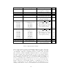
been implemented by extending the NuSMV model checker [4]. The results table
(Table 1) contains four columns. The first two columns contain the description
and size (number of states) of the participating protocols . The ACTL properties
used are shown in the third column with the size of the converter shown in
column 4. The first five problems are well-known protocol conversion problems
with control mismatches [10, 7]. The next problem is the multi-write producer
and single-read consumer protocol pair used as the motivating example in this
paper. The size of the output of the producer was kept constant at 8-bits and
the input-size of the consumer were varied in multiples of 8-bits and the size
of the converter is noted in the fourth column. Note that when the input size
was not a direct multiple of the output size (9-bits and 2-bits respectively),
no converter could be generated. This was due to the fact that the consumer
13
P1 (|SP1 |)
Master (3)
P1 (|SP2 |)
Slave (3)
ABP sender(6)
ABP receiver(8)
Poll-End Receiver(2)
NP receiver(4)[7]
NP sender(3)[7]
Ack-Nack Sender(3)
Handshake (2)
Serial(2)[10]
Multi-write
Producer protocol(3)
8-bit Write
8-bit Write
8-bit Write
8-bit Write
2-bit Write
Multi-write
Producer protocol(3)
2-bit Write
2-bit Write
3-bit Write
3-bit Write
9-bit Write
7-bit Write
11-bit Write
Mutex Process 1 (3)
MCP missionaries
4-bit ABP Sender
Single-read
Consumer protocol(4)
8-bit Read
16-bit Read
24-bit Read
32-bit Read
9-bit Read
Multi-read
Consumer protocol(4)
9-bit Read
11-bit Read
10-bit Read
11-bit Read
2-bit Read
64-bit Read
256-bit Read
Mutex Process 2(3)[4]
MCP cannibals (30)[4]
Modified Receiver (166432)[4]
ACTL Properties
Event sequencing
(one grant per request),
(requests precede grants)
Control Signal matching
Control signal matching
Data communication resolution
(one data in per data out)
Control signal matching
and event sequencing
(Alternating A and B labels)
AG(¬Error),A(¬D Out U Req In)
A(¬Req In U R Out)
(Error is never encountered,
no data written before requests,
and no requests read before
any requests are made)
AG(¬Error),A(¬D Out U Req In)
A(¬Req In U R Out)
(Error is never encountered,
no data written before requests,
and no requests read before
any requests are made)
Mutual exclusion
N ummissionaries ≥ N umcannibals
Liveness checking based on
control signal matching
Table 1: Implementation Results
allowed only a single read after each handshake with the producer. The next
set of results were obtained when the consumer allowed multiple reads with
each handshake. This allowed handling arbitrary read-write pairs. The final
three results are well-known NuSMV examples modified to create mismatches.
The mutex example was modified such that a violation of the mutual exclusion
property occurred. The missionaries and cannibals problem, an abstraction of
data-communication between two protocols was also handled successfully. It
involved constraining data-communication between protocols such that size of
the communication medium (boat) was not exceeded, and at the same time,
further restrictions on data-variables (number of cannibals never exceeds the
number of missionaries) were also handled. The 4-bit alternating-bit protocol
example, was modified to create a control mismatch between the sender and the
14
C(|SC |)
6
8
8
6
3
8
11
13
15
Failed
25
29
28
30
11
140
528
7
22
14312
receiver, which introduced many faulty paths in the combined system. Using the
tableau construction algorithm, a converter that effectively disabled such faulty
communication paths was realized. Note that size entry in the second column
for the final two results is the combined size of the system (size of P1 ||P2 ).
4
Conclusions
Protocol conversion to resolve protocol mismatches is an active research area
and a number of solutions have been proposed. Some approaches require significant user effort, while some only partly address the protocol conversion problem.
Most formal approaches work on protocols that have unidirectional communication and use finite state machines to describe specifications. In this paper
we propose a formal approach to protocol conversion which alleviates the above
problems. Specifications are described in temporal logic and bidirectional communication is allowed. A tableau-based approach using the model checking
framework is used to generate converters in polynomial time. We use invariants to handle data-width issues. Fairness properties are used to generate fair
converters. We prove that the approach is sound and complete and provide
implementation results.
References
[1] Rajeev Alur and David L. Dill. A theory of timed automata. Theoretical
Computer Science, 126(2):183–235, 1994.
[2] Girish Bhat, Rance Cleaveland, and Orna Grumberg. Efficient on-the-fly
model checking for CTL*. In Proceedings of the Tenth Annual Symposium
on Logic in Computer Science, pages 388–397, June 1995.
[3] Vijay D’Silva, S Ramesh, and Arcot Sowmya. Synchronous protocol automata : A framework for modelling and verification of soc communication
architectures. In DATE, pages 390–395, 2004.
[4] R. Cavada et al. NuSMV 2.1 User Manual, June 2003.
[5] Saurav Gorai et al. Session 42: simulation assisted formal verification: Directed-simulation assisted formal verification of serial protocol and
bridge. In Proceedings of the 43rd annual conference on Design automation
DAC ’06, pages 731 – 736, 2006.
[6] P. Green. Protocol conversion. IEEE Transactions on Communications,
34(3):257–268, March 1986.
[7] S Lam. Protocol conversion. IEEE Transactions on Software Engineering,
14(3):353–362, 1988.
15
[8] F. Maraninchi and Y. Remond. Argos: an automaton-based synchronous
language. Computer Languages, 27:61–92, 2001.
[9] K. Okumura. A formal protocol conversion method. In ACM SIGCOMM
86 Symposium, pages 30–37, 1986.
[10] R. Passerone, L. de Alfaro, T. A. Henzinger, and A. L. SangiovanniVincentelli. Convertibility verification and converter synthesis: Two faces
of the same coin. In International Conference on Computer Aided Design
ICCAD, 2002.
[11] J. C. Shu and Ming T. Liu. A synchronization model for protocol conversion. Proceedings of the Eighth Annual Joint Conference of the IEEE
Computer and Communications Societies. Technology: Emerging or Converging? INFOCOM ’89, pages 276–284, 1989.
[12] R Sinha, P Roop, and S Basu. Automatic synthesis of converters for protocol matching using model checking. Technical Report 00000482, Iowa State
University, 2006.
16