Download Local Module Checking for CTL Specifications

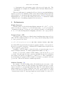
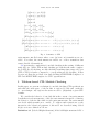
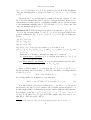
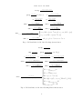
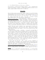
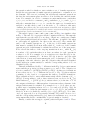
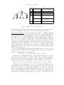
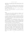
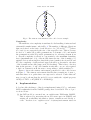
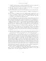
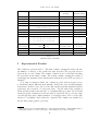
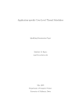
FESCA 2006
Local Module Checking for CTL Specifications
Samik Basu
1
Department of Computer Science
Iowa State University
Ames, USA
Partha S Roop 2
Department of Electical and Computer Engineering
University of Auckland
Auckland, New Zealand
Roopak Sinha 3
Department of Electical and Computer Engineering
University of Auckland
Auckland, New Zealand
Abstract
Model checking is a well known technique for the verification of finite state models
using temporal logic specification. While model checking is suitable for transformational systems (also called closed systems), it is unsuitable for open systems (also
known as reactive systems) where the nondeterminism in the environment must be
considered during verification. Module checking is an approach for the verification of
open systems which have both closed (internal) and open (environment or external)
states. It has been demonstrated in [10] that the complexity of module checking
branching time logic CTL is EXPTIME-complete. The approach to module checking is global and the method tries to establish that the property in question holds
over all possible environments.
This papers develops a local approach to CTL module checking using tableau
rules. The proposed approach tries to determine a single environment under which
the negation of the property is satisfied over the given module. Such a strategy,
thus, leads to a local approach to module checking where we only explore states
that are relevant to proving that the negation of the property can be satisfied over
the given module using an appropriate witness (environment) that the algorithm
also generates. While the worst case complexity of our algorithm is identical to the
This paper is electronically published in
Electronic Notes in Theoretical Computer Science
URL: www.elsevier.nl/locate/entcs
Basu, Roop and Sinha
earlier complexity, we demonstrate that practical implementation of the proposed
approach is feasible and yields much better results than the global approach.
Key words: module checking, open systems, tableau based
verification
1
Introduction
Reactive systems [7,13] are open systems that continuously interact with their
environment while executing a non-terminating control program. Examples
include operating systems, communication protocols, missile and avionics systems and controllers for nuclear plants and simple home appliances such as
microwaves, DVD players and washing machines. Such applications require
careful analysis, design and validation techniques as they can often be safety
critical. Hence, formal techniques have often been used in the design, development and validation of these systems [16,11,5,6,3,12,15]. Formal techniques
use precise syntax and semantics for defining specifications and models of systems so that rigorous verification of properties such as correctness, reliability
and security is made possible.
With the advent and widespread use of embedded systems, which are ubiquitous reactive computing systems ranging from simple home appliances to
very complex applications in avionics and defense, the need for formal methods in the design of reactive systems is growing. One very common approach
to verification of reactive systems has been model checking. A model checker
takes a formula in some temporal logic [14] as a desirable property and performs formal analysis over a finite-state model of a system (called a Kripke
structure [3], a special class of finite state machines). The model checking
process is essentially an automated reachability analysis task over the finite
state model of the system. This task either terminates with a proof that
the temporal property holds over the model or on failure generates a counter
example.
The model checker, during the reachability analysis phase, assumes that
all transitions out of any given state of a model is eventually enabled. This
assumption is based on the fact that the model is considered to be closed i.e.,
all states of the system are purely internal and that it is the system that gets
to choose which transition to take based on some internal computation. This
approach to analysis, while being suitable for transformational systems which
are closed, are unsuitable for reactive systems that are open.
An open system maintains an ongoing interaction with its environment.
Hence, the state-space of such a system may be partitioned into a set of
1
2
3
Email: [email protected]
Email: [email protected]
Email: [email protected]
2
Basu, Roop and Sinha
states that are open (also called external or environment states) and another
set of states that are closed (also called internal or system states) [8,9]. An
environment state reacts to events in the external environment of the open
system and the environment is considered asynchronous and uncontrollable. A
system state, on the other hand, takes no inputs from the external environment
and the system automatically chooses one of the transitions based on some
internal decision (such as say the value of a variable or the result returned by
a function). Kupferman et al. have recently shown that model checking may
not be enough for open systems due to the presence of environment states and
when branching formulas are considered in the specification [9]. The proposed
technique, called module checking, takes the asynchronous environment into
account while doing a proof for branching-time logics. [6,5] further discuss
techniques devoted to issues concerning verification of open systems.
This paper illustrates the need for module checking reactive systems and
proposes an alternate approach to module checking that has efficient implementation avenues compared to the original approach. We first illustrate the
need for module checking followed by our approach to local module checking.
1.1
Motivating Example - The Coffee Brewer Verification Problem
Consider a simple coffee brewer model as depicted in the Figure 1. In this
figure, environment states are shown using elipses whereas system states are
drawn as circles. Each transition out of any state is marked by a natural
number starting with 1. The brewer serves either five or ten cups of coffee
in either medium or strong flavor. A user can select the number of cups of
coffee (using a switch as an input) and the strength of coffee (using another
switch). The brewer is normally in the off state until the switched on. Hence,
the initial state labeled by the proposition OF F is an environment state.
Once the brewer is switched on, it enters a state labeled by the proposition
CHOOSE. This is again an environment state. In this state, the user can
select the number of cups of coffee and the strength of coffee. Depending on the
selection (two switches lead to four different possibilities), the brewer enters
any one of the following states: (f ive, medium), (f ive, strong), (ten, medium)
or (ten, strong). Once the selections have been made and the corresponding
state has been reached, the brew cycle switch has to be switched on to start
the brewing. Hence all the above four states are also environment states. Once
the brew cycle is set, the brewer makes a transition to a state labeled BREW .
This state is a system state since no inputs from the environment is required
to make progress. From the BREW state, the brewer makes an automatic
transition to the DON E state after a predetermined time period (which is the
amount of time taken by the brewing process). The state labeled DON E is
also a system state since the brewer takes one of two possible branches based
on some internal condition. If any error is detected (say not enough coffee
or no milk power), then a transition is made to an error state (labeled by
ERROR). Alternatively, the brewer can reach a state labeled SERV E where
3
Basu, Roop and Sinha
s0
OFF
s1
1
CHOOSE
1
s2
s3
FIVE, MED
s4
2
FIVE, STR
TEN, MED
TEN, STR
1
1
1
1
s5 4
3
s6
1
1
BREW
s
1
7
DONE
2
1
s8
s9
ERROR
SERVE
Fig. 1. The coffee brewer example
the actual coffee selected is served.
CTL is a branching time temporal logic that has been shown to be quite
efficient for model checking. Let us consider the following CTL property:
AGEF (T EN ∧ AF (SERV E ∨ ERROR)) which demands that from any
state one can possibly eventually select ten cups of coffee and once selected,
ten cups will always be served (or an error encountered) in the future.
Note that a model checker will always return a true answer for this question. However, consider the following situation. Due to cost cutting in the
work place where the brewer is installed, brewing ten cups of coffee at a time
is not allowed (this has been enforced through a circular and the ten cups
switch is masked). Hence, no user will be allowed to make this selection from
the CHOOSE state. Thus, it will not be possible to guarantee the selection
of ten cups of coffee and hence the property fails to hold over the coffee brewer
model. This property could also be violated if all users request five cups of
coffee or tea (and no users request ten cups of any beverage). In this case,
even though the machine is capable of dispensing ten cups of tea or coffee, the
environment in which it operates effectively disables it from doing that.
This property illustrates that due to the presence of environment states, it
may not be always possible to satisfy branching time temporal properties. As
the environment of an open system is asynchronous and hence uncontrollable,
the environment may never enable some desired transitions leading to failure
of the property. This example thus motivates the module checking problem:
how do we ensure that a given property holds over a known module (a model
with environment and system states) assuming an uncertain environment.
The basic idea in module checking is to prove that the property holds over all
4
Basu, Roop and Sinha
possible choices made in the environment states. In other words, the module
checking problem is to decide if a CTL formula ϕ holds over a module M
provided for all possible environments E such that M × E satisfy ϕ. Here,
M × E denotes the composition of the model and the environment running in
parallel (to be formalized later).
This may be expressed as follows: module checking, denoted by M |=o ϕ,
therefore, amounts to deciding whether ∀E.M × E |= ϕ; i.e.
M |=o ϕ ⇔ ∀E.M × E |= ϕ
(1)
It has been shown in Kupferman et al. [10] that the module checking problem for the temporal logic CTL is EXPTIME-complete unlike the polynomial
complexity for the model checking problem. The reason for this complexity may be intuitively seen from the above equation since the proof has to
be carried out for all possible environments. This is unlike model checking,
where the system is closed and hence the reachability proof proceeds without
considering any nondeterminism in the environment.
While this sounds like bad news, a practical implementation of module
checking is possible by the following observation.
Proceeding further, from Equation 1 we state that
M 6|=o ϕ ⇔ ∃E 0 .(M × E 0 6|= ϕ ⇔ M × E 0 |= ¬ϕ)
(2)
In the above, the negation on ϕ can be pushed inside the formula such that all
temporal and boolean operators are free from negation. Furthermore as the
existence of E 0 ensures that M 6|=o ϕ, E 0 acts as a witness to the violation. Such
a witness can be used to provide useful insights to the reason for violation of
a desired property over an open systems. The main beauty of this procedure
is that we are looking for only one environment using which we can prove
that the formula is not satisfied. We will illustrate later that we can employ
a set of tableau rules to perform the computation of E 0 locally. This local
computation is similar to on-the-fly model checking [1] where the state space
of the system under verification is constructed on a need-driven basis. Even
though the worst case complexity of local module checking is still bounded
by the results of [10], we demonstrate that the proposed approach to local
module checking yields much better practical results. The main contributions
of this paper are:
(i) We propose a set of sound and complete tableau rules for local module
checking. The proposed approach determines a single witness (environment) so that under the witness the negation of the given CTL property
is satisfied. The proof proceeds only along a local set of states that are
needed for the generation of a witness.
(ii) We have developed a local module checker by extending NuSMV [2].
Local module checking has been compared with the generation of the
maximal environment under which the given CTL property is satisfied
5
Basu, Roop and Sinha
to demonstrate the performance gain of the proposed approach. The
benchmarks are examples from NuSMV with both environment and system states.
The rest of this paper is organized as follows. Section 2 presents fundamental theory. Section 3 formulates CTL local module checking and presents the
tableau rules for both system and environment states. Section 4 describes the
implementation of a local module checker and section 5 contains the results
obtained from it. Concluding remarks follow in section 6.
2
Preliminaries
Kripke Structure.
System behavior is described using Kripke structure M = (S, s0 , →, P, L),
where S is the set of states, s0 ∈ S is the start state, →⊆ S × S is the set
of transition relations, P is the set of propositions relevant to M and finally,
L : S → 2P is the labeling function mapping each state to set of propositions.
Temporal logic: CTL.
Properties of the system are defined using branching time temporal logic
CTL. A CTL formula is defined over a set of propositions using temporal and
boolean operators as follows:
φ → P | ¬P | tt | ff | φ ∧ φ | φ ∨ φ | AXφ | EXφ | A(φUφ) | E(φUφ) | AGφ | EGφ
Note that CTL in general allows negations on temporal and boolean operators.
However, we restrict ourselves to verifying CTL formulas where negations can
only be applied to propositions.
Semantics of CTL formula, ϕ denoted by [[ϕ]]M is given in terms of set of
states in Kripke structure, M , which satisfies the formula. See Fig. 2.
A state s ∈ S is said to satisfy a CTL formula ϕ, denoted by M, s |= ϕ, if
s ∈ [[ϕ]]M . We will omit M from |= relation and [[]] if the model is evident in
the context. We will also say that M |= ϕ iff M, s0 |= ϕ. The complexity for
model checking M against a CTL formula ϕ is O(|M | × |ϕ|) where |M | and
|ϕ| are size of the model and the formula respectively.
Module Checking. [8]
In contrast to model checking where all transitions in every state of the
model are always enabled, module checking is specifically directed for verification of models of open systems with states where the environment decides
which transitions are enabled. Typically, in models of open systems, modules
in short, the states are partitioned into two sets Ss and Se where Ss consists
of system states with all outgoing transitions enabled while Se is the set of
6
Basu, Roop and Sinha
[[p]]M ={s | p ∈ L(s)}
[[¬p]]M ={s | p 6∈ L(s)}
[[tt]]M =S
[[ff]]M =Φ
[[ϕ ∧ ψ]]M =[[ϕ]]M ∩ [[ψ]]M
[[ϕ ∨ ψ]]M =[[ϕ]]M ∪ [[ψ]]M
[[AXϕ]]M ={s|∀s → s0 ∧ s0 ∈ [[ϕ]]M }
[[EXϕ]]M ={s|∃s → s0 ∧ s0 ∈ [[ϕ]]M }
[[A(ϕU ψ)]]M ={s|∀s = s1 → s2 → . . . ∧ ∃i, j.sj |= ψ ∧ ∀i < j.si |= ϕ}
[[E(ϕU ψ)]]M ={s|∃s = s1 → s2 → . . . ∧ ∃i, j.sj |= ψ ∧ ∀i < j.si |= ϕ}
[[AGϕ]]M ={s|∀s = s1 → s2 → . . . ∧ ∀i.si |= ϕ}
[[EGϕ]]M ={s|∃s = s1 → s2 → . . . ∧ ∀i.si |= ϕ}
Fig. 2. Semantics of CTL
environment-controlled states where some (at least one) transitions are enabled. Note that, the environment can enable one or more transitions but
cannot disable all transitions.
[10] presents the complexities for module checking in the setting of different
temporal logic. While LTL module checking problem has the same complexity as LTL model checking, module checking branching-time temporal logics
(CTL, CTL*) is harder compared to corresponding model checking. It has
been proved that the problem of module checking is EXPTIME-Complete for
CTL and 2EXPTIME-complete for CTL* specifications.
3
Tableau-based CTL Module Checking
In this paper, we present a technique for module checking CTL specifications
such that the state-space of the module is explored locally and on-the-fly,
i.e. our technique only explores the states needed to (dis)satisfy a given CTL
formula.
We consider the behavior of a module M in the context of an environment
E such that at each system state of M, the environment is incapable of altering
the behavior of the module while at each environment state, the environment
can decide which transitions to enable. To address such restrictions on the
interaction, the behavioral patterns of M and E are described using labeled
Kripke structure defined as follows:
Definition 3.1 [Labeled Kripke Structure] A labeled Kripke structure LKS =
7
Basu, Roop and Sinha
(S, s0 , →, P, L, K) where S, s0 , P, L are defined as before, K is the maximum
out-going branching factor of states in S and →⊆ S × {1, 2, . . . , n} × S with
n ≤ K.
The state set S of a module may be partitioned into two subsets, S e , the
set of all environment states and S s , the set of all system states. In the above,
each transition is annotated by a branching identifier whose domain is equal
i
to the maximum branching factor. We will write s → s0 to denote the i-th
out-going transition from s if (s, i, s0 ) ∈→.
Definition 3.2 [Parallel Composition] Given a module M = (SM , s0M , →M
, PM , LM , K), its environment E = (SE , s0E , →E , PE , LE , K), their parallel composition resulting in M × E ≡ P = (SP , s0P , →P , PP , LP , K) are defined as
follows
(i) SP ⊆ SM × SE
(ii) s0P = (s0M , s0E )
(iii) PP = PM ∪ PE
(iv) LP (s1 , s2 ) = LM (s1 ) ∪ LE (s2 ) where s1 ∈ SM and s2 ∈ SE
i
i
i
(v) (s1 , s2 ) →P (s01 , s02 ) if s1 →M s01 and s2 →E s02 where s1 , s01 ∈ SM and
s2 , s02 ∈ SE
Furthermore, following constraints are imposed to restrict E
i
(a) System-state conformity. if s1 is a system state then ∀s1 →M s01 ⇒
i
∃s2 →E s02 and vice versa.
(b) Environment-controllability. if s1 is an environment-controlled state
i
j
j
then ∃s2 →E s02 ∧ (∀s2 →E s002 ⇒ ∃s1 →M s001 )
Given a CTL formula ϕ, we say that M × E ≡ P |= ϕ ⇔ s0P |= ϕ.
Module checking, denoted by M |=o ϕ, therefore, amounts to deciding whether
∀E.M × E |= ϕ; i.e.
M |=o ϕ ⇔ ∀E.M × E |= ϕ
(3)
Proceeding further, from Equation 3 we state that
M 6|=o ϕ ⇔ ∃E 0 .(M × E 0 6|= ϕ ⇔ M × E 0 |= ¬ϕ)
(4)
It is important to note however that M 6|=o ϕ 6⇒ M |=o ¬ϕ. It can be
shown that a module does not satisfy both a formula and its negation 4 . A
module might satisfy a formula and its negation under different environments.
1
2
1
1
For example: given M = ({s0 , s1 , s2 }, s0 , {s0 → s1 , s0 → s2 , s1 → s1 , s2 →
s2 }, {p}, L, 2}) where L(s1 ) = {p} and CTL formula AXp, it is easy to see
that M 6|=o AXp and M 6|=o EX¬p.
4
Note that the same is not true for model checking problem: M 6|= ϕ ⇔ M |= ¬ϕ
8
Basu, Roop and Sinha
ss |e |= {ϕ1 ,...,ϕn }
ss |e |= ϕ1 ... ss |e |= ϕn
reorg
ss |e |= p
.
prop
∨1
unreu
∧
ss |e |= ϕ1 ∨ϕ2
ss |e |= ϕ1
∨2
ss |e |= ϕ1 ∧ϕ2
ss |e |= ϕ1
ss |e |= ϕ2
ss |e |= ϕ1 ∨ϕ2
ss |e |= ϕ2
ss |e |= E(ϕU ψ)
ss |e |= ψ∨(ϕ∧EXE(ϕU ψ))
unrau
ss |e |= A(ϕU ψ)
ss |e |= ψ∨(ϕ∧AXA(ϕU ψ))
ss |e |= EGϕ
ss |e |= ϕ∧EXEGϕ
unrag
ss |e |= AGϕ
ss |e |= ϕ∧AXAGϕ
unreg
unrss ,ex
p ∈ L(ss )
ss |e |= EXϕ
si |ei |= ϕ, sj |ej |=tt...sk |ek |=tt
unrss ,ax

I
 s ∈ N S = {s |s →
i
I
M sI }, sj,...,k ∈ N S − {si }
I
e
∈ N S = {e |e → e }
i,j,...,k
ss |e |= AXϕ
s1 |e1 |= ϕ ... sk |ek |= ϕ
e
I
E
I
i
i
∀1 ≤ i ≤ k.ss →M si ∧ e →E ei
Fig. 3. Tableau Rules for Module Checking System States
reorg
emp
∧
unreu
se |e |= {ϕ1 ∧ϕ2 ,C}
se |e |= {ϕ1 ,ϕ2 ,C}
prop
∨1
se |e |= {p,C}
se |e |= C
se |e |= {ϕ1 ∨ϕ2 ,C}
se |e |= {ϕ1 ,C}
p ∈ L(se )
∨1
se |e |= {ϕ1 ∨ϕ2 ,C}
se |e |= {ϕ2 ,C}
se |e |= {E(ϕU ψ),C}
se |e |= {(ψ∨(ϕ∧EXE(ϕU ψ))),C}
unrau
se |e |= {A(ϕU ψ),C}
se |e |= {(ψ∨(ϕ∧AXA(ϕU ψ))),C}
se |e |= {EGϕ,C}
se |e |= {ϕ∧EXEGϕ,C}
unrag
se |e |= {AGϕ,C}
se |e |= {ϕ∧AXAGϕ,C}
unreg
unrse
se |e |={}
.
se |e |= ϕ
se |e |= {ϕ}
se |e |= C
∃π⊆Π. ∃ΠCex (π). ∀i∈π. si |ei |=Cax ∪Ci

S

Cax = AXϕk ∈C ϕk





S


Cex = EXϕl ∈C ϕl




i
 Π = {i | s →
e
M si }


ΠCex (π) = {Ci | i ∈ π ⊆ Π ∧ Ci ⊆ Cex }




S


Cex = i:Ci ∈ΠCex (π) Ci




T
i:Ci ∈ΠCex (π) Ci = Φ
Fig. 4. Tableau Rules for Module Checking Environment States
9
Basu, Roop and Sinha
3.1
Local Module Checking and Generation of Witness
We present here a tableau-based technique similar to [4] for constructing the
witness environment E, existence of which ensures that the module does not
satisfy original formula. Tableau rules are defined as
Antecedent
Consequent
where the Antecedent represents the current obligation for module checking
and Consequent denotes the next obligation. A successful tableau (see below)
will result in automatic generation of the environment E. Figs. 3 and 4 present
the complete tableau where the former corresponds to the rules for system
states and the latter for the environment-controlled states.
Tableau for System States. Consider first the Fig. 3 (without the reorg rule).
The rules for prop, ∧, ∨s are simple and intuitive. The prop rule leads to
a successful tableau leaf, the ∧ rule is successful if both its consequents are
successful and finally, the success of ∨-rule depends on the success of any of
its consequents. The rule unreu corresponds to unrolling of the EU formula
expression. A state satisfies E(ϕU ψ) iff (a) ψ is satisfied in the current state
or (b) ϕ is true in the current state and in one of its next states E(ϕU ψ) is
satisfied. The rule for unrau is similar to unreu with exception of the presence
of universal quantification on the next states (AX). The rule unreg (unrag )
states that the current state satisfies ϕ and in some (all) next state EGϕ
(AGϕ) holds true.
Finally, the rules for unrss ,ex and unrss ,ax correspond to the unfolding of
the state and the formula expression simultaneously. Note that in the former,
we are searching for at least one next state, while in the latter all next states
should satisfy ϕ. As such for the EX-formula expression, the tableau selects
any one of the next states si |ei and if the selected state satisfies ϕ, there is no
obligation left for the rest of the next states; the obligations on the remaining
next states sj,...,k in the context of the environment is to satisfy tt 5 (any state
satisfies the propositional constant tt). Note that, the tableau can potentially
have k sub-tableaus for unrss ,ex each of which will correspond to selection of
one next state si from the set of k next states of ss .
Observe that, the rules unrss ,ex , unrss ,ax lead to one-step construction of
the environment. Conforming to the constraint that the environment at the
system state cannot control the enabled transition, the environment must have
exactly the same number of transitions as the system state.
Tableau for Environment-Controlled States. The tableau rules (Fig. 4) for environment controlled states are slightly different from the one described above.
Instead of asking whether a state satisfies a formula expression (see Fig. 3),
5
For the purpose of constructing the environment, in Rule unrss ,ex , we can safely assume
that all the environment states ej...,k replicates the behavioral patterns of module states
sj...,k .
10
Basu, Roop and Sinha
the question asked is whether a state satisfies a set of formula expressions.
In fact the set represents a formula expression equivalent to conjunction over
its elements. The reason for altering the tableau rule structure stems from
the fact the environment plays an active role in deciding the enabled transitions. For example: in order to construct an environment state e such that
se |e |= ϕ∧ψ, we need to construct e1 and e2 such that se |e1 |= ϕ and se |e2 |= ψ
with the constraint that e1 = e2 , i.e. exactly the same set of transitions is
enabled to module check ϕ and ψ at the state se . To address to this state
of affairs, the tableau rules for environment-controlled state maintains a global
view of all the formula to be satisfied and ensures consistent enabling/disabling
of transitions by the environment (to be constructed).
The rules for prop, ∨, unreu , unrau , unreg , unrag in Fig. 4 are similar to that
in Fig. 3. The rule for ∧ aggregates all the conjuncts in the set. The emp-rule
represents the case the state does not have obligation to satisfy any formula
and a (successful) tableau leaf is reached. The rule unrse is applied only when
no other rules are applicable. In other words, the set C only contains EX
and/or AX formula expressions. Cax is the set of all formula expressions
that must be satisfied in all next states while Cex is the set of the formula
expressions each of which must be satisfied in at least one of the next states.
Π records all the indices of the outgoing transitions from se , while ΠCex (π)
is a subset of Cex such that there is at least one subset for each i present in
a subset π ∈ Π. For example, if π is a singleton set, then ΠCex (π) is also
a singleton set containing Cex . In short, ΠCex (π) is used to associate with
i-th selection of next state-environment pair a set of elements Ci ⊆ Cex . The
consequent of the rule, therefore, fires the obligation that all states identified
by the indices in π must satisfy Cax and the corresponding subset of Cex as
identified by ΠCex (π).
This rule is illustrated by Fig. 5. All states in the Fig. 5(a) are environment
states and the proposition p is true at states s1 , s4 , and s6 . The obligation at
s0 |e0 is to satisfy C = {AXEXp, EXEX¬p, EXp}. As there are 3 transitions
from s0 there are 23 − 1 = 7 different choices for π. Fig. 5(b) shows subsets
consisting of only 1 and 2. π represents the indices of enabled transitions.
These transitions lead to states which must satisfy all the elements of Cax =
{EXp}. Corresponding to each π, there exists at least one choice for ΠCex (π)
which subsets Cex = {p, EX¬p} in |π| subsets where |π| is the size of π. It
also assigns each subset to different subset of next states where elements of the
assigned subset must be satisfied. For example for π = {1, 2}, there are two
possible ways of assigning subsets of Cex to s1 |e1 and s2 |e2 (see Fig. 5(b)). In
this example, we obtain an environment e0 for π = {1, 2} (i.e. the transition
labeled 3 from s0 is disabled), and ΠCex (π) = {{p}, {EX¬p}}. Note that,
our local approach does not necessarily examine all possible choices for π
and the corresponding subsets ΠCex (π); instead it terminates as soon as an
environment that leads to satisfiability of given formula is obtained.
Finally, consider the reorg (re-organize) rules in Figures 3 and 4. These
11
Basu, Roop and Sinha
Antecedent: s0 |e0 |= C
Cax = {EXp}, Cex = {p, EX¬p}
Consequent
ΠCex (π)
π
si |ei |= Cax ∪ Ci
S0
1
2
p S1
1
S4 p
2
S5
3
S2
1
S6 p
S3
{1}
{Cex }
s1 |e1 |= {EXp, EX¬p, p}
{2}
{Cex }
s1 |e1 |= {EXp, EX¬p, p}
1
2
S7
S8
{{p},{EX¬p}}
√
{1,2}
{{EX¬p},{p}}
.
.
.
(a)
s1 |e1 |= {EXp, p}
s2 |e2 |= {EXp, EX¬p}
s1 |e1 |= {EXp, EX¬p}
s2 |e2 |= {EXp, p}
(b)
Fig. 5. Illustration of unrse tableau rule
rules rearrang the formula obligations from set-based to expression-based or
vice versa depending on the type of the model state being considered.
Finitizing the Tableau. The given tableau rules can be of infinite depth as
each recursive formula expressions AU, EU, AG, EG are unfolded infinitely
many times. However, the total number of states in the Kripke structure for
the module is N = |S|, and this finitizes the tableau depth. In Fig. 3, if the pair
(ss , ϕ) in ss |e |= ϕ, where ϕ is either EG or AG formula expression, appears
twice in a tableau path, we fold back the tableau by pointing the second
occurrence to the first and stating a successful tableau loop is obtained. Note
that this also leads to generation of a loop in the constructed environment.
On the other hand, if the pair (ss , ϕ), where ϕ is of the form EU or AU ,
appears twice, the second occurrence is classified as an unsuccessful tableau
leaf and is replaced by ff.
The idea of folding back or replacing using false relies on fixed point semantics of CTL formulas. The CTL formulas EG and AG can be represented
by greatest fixed point recursive equations:
EGϕ ≡ Z =ν ϕ ∧ EXZ
AGϕ ≡ Z =ν ϕ ∧ AXZ
In the above ν represents the sign of the equation and is used to denote
greatest fixed point and Z is recursive variable whose valuation/semantics
(set of model states) is the greatest fixed point computation of its definition.
Similarly the fixed point representation of CTL formulas AU and EU are
E(ϕU ψ) ≡ Z =µ ψ ∨ (ϕ ∧ EXZ) A(ϕU ψ) ≡ Z =µ ψ ∨ (ϕ ∧ AXZ)
The fixed point computation proceeds by iteratively computing the approximations of Z over the lattice of set of states in the model. A solution is
reached only when two consecutive approximations are identical. For greatest
fixed point computation, the first approximation is the set of the all states
(top of the lattice) and as such a system can satisfy a greatest fixed point
formula along an infinite path (using loops). On the other hand, the first
12
Basu, Roop and Sinha
approximation of the least fixed point variable is empty set (bottom of the
lattice) and therefore satisfiable paths for least fixed point formula are always
of finite length.
For the tableau in Fig. 4, the finitization condition is similar. If the pair
(se , C) in se |e |= C, appears twice in a tableau path and if C contains any least
fixed point CTL formula expression, then the second occurrence is replaced
by ff ; otherwise the second occurrence is made to point to the first and a
successful tableau is obtained.
Theorem 3.3 (Sound and Complete) Given a module M and CTL formula ϕ, M 6|=o ϕ, iff the tableau in Figures 3 and 4 generates an environment
E where M × E |= ¬ϕ.
Proof.
The proof proceeds by realizing the soundness and completeness of each
of the tableau rules. For brevity, we present here the proof-sketch for unr se ,
proofs for the other rules are straightforward.
Recall that, se |e |= C, where C is the set of formula expressions with temporal operators AX and EX, is satisfiable if the next states proof obligations
are satisfied by destination states reachable via transitions enabled by the
environment e. The environment can enable any subset (barring ∅) of transitions. The tableau rule, therefore, considers all possible subset of destination
states of enabled transitions.
As each transition is annotated by an index (whose domain is over the outgoing branching factor of se ), we construct Π, the set of indices of out-going
transitions. In other words, i ∈ Π ⇒ si is reachable via the transition with
index i. We are required to identify one possible subset of Π which represents
the enabled transitions whose destinations conform to the satisfiability obligations in the consequent (see ∃π ⊆ Π in the consequent). Let πs = {si | i ∈ π}
be the next states reachable via (selected) enabled transitions.
The consequent of the tableau rule has the following obligations. All elements of πs in parallel composition with the environment must satisfy the
expressions in Cax and for each formula expression ϕ in Cex , there must be
at least one state which in conjunction with the corresponding environment
satisfies ϕ. Observe that, there is requirement for an existence of a subset,
ΠCex (π), of Cex corresponding to a subset π such that next state-environment
pairs satisfy the corresponding obligations. This ensures that the environment constructed is consistent, i.e., ei is constructed such that si |ei satisfies
both the for all obligations (Cax ) and its share of existential obligations (Ci ).
Therefore, if we can generate an environment for se corresponding to rule
unrse , then se 6|=o ψ where ψ is the disjunction of the elements of the set
{AX¬ϕ | ϕ ∈ Cex } ∪ {EX¬ψ | ψ ∈ Cax }. The other direction can be proved
likewise.
2
13
Basu, Roop and Sinha
Fig. 6. The witness environment for the coffee brewer example
Complexity.
The main factor in complexity is attributed to the handling of universal and
existential formulas in unrse rule in Fig. 4. The number of different obligations
that can be fired on the basis of each selection of π ⊆ Π, is O(2|Cex |×|π| ) where
|Cex | and |π| are respectively the size of the respective sets. This is because
we need to consider all possible permutations of elements of Cex and match
the permutations with all possible permutations for selecting element from
π. Overall complexity is, therefore, exponential to the maximum branching
factor (maximum size of π) of the module times the size of the formula to be
satisfied. It is worth noting here that if the given formula is free from EX and
EU , the complexity of tableau-based approach will be polynomial to the sizes
of the formula and module (same as model checking). This is due to the fact
that in the presence of only AX-formulas in rule unrse , we are only required
to find one element from Π; the state corresponding to which satisfies Cax .
Figure 6 shows the witness environment generated for the coffee brewer
in Figure 1. The witness environment disables three transitions of state s1
such that there is no path where ten cups can be selected. Under this witness, it can be shown that the model does not satisfy the original property
AG E(tt U T EN ∧ AF (SERV E ∨ ERROR)).
4
Implementation
A local module checking tool has been implemented using C/C++ and many
SMV benchmarks from the NuSMV package have been tested. The tool proceeds as follows:
(i) An SMV model is converted into an explicit state FSM using NuSMV.
This is achieved by traversing the model’s state space in NuSMV and
writing all reachability information (states, transitions and labels) to
a file. As there is no explicit notion of system/environment states in
14
Basu, Roop and Sinha
NuSMV, the state space is divided randomly into two sets of equal size
representing system and environment states respectively.
(ii) The file containing the explicit state FSM is read by the tool along with
the CTL property to be used for verification.
(iii) The CTL property is negated and the negation is carried inwards. CTL
properties can not have negations applied to formulas other than propositions.
(iv) A search for a witness is carried out, starting with the initial state, and
the tool attempts to generate an environment under which the module
satisfies the negated CTL property. If a witness is present, then the
module does not satisfy the original property.
The algorithm applies the appropriate system or environment state tableau
rules on the current state. Once all present (current-state) commitments are
met, any future commitments are passed to its successors. It uses a heuristic to
compute a small set of successors of the current state which satisfy all its future
commitments. This is used to ensure that the generated witness is small. If
no witness can be computed, it can be concluded that the module satisfies the
CTL property. Note that the algorithm attempts to generate a small witness
and not the minimal witness for a given property and module. In order to
compare the obtained results, the tool was extended to find an environment
under which the original CTL property is satisfied. This is achieved as follows:
(i) The CTL property (non-negated) is read along with the module FSM (as
above).
(ii) The algorithm attempts to find an environment under which the given
CTL property is satisfied by traversing all of the reachable state space.
It is important to note here that the above is not an implementation of
global module checking. Global module checking advocates the need to check if
the given property is satisfied by the module under all environments. However,
the above approach constructs only a single environment under which the given
CTL property is satisfied by the module. However, unlike the local module
checker which attempts to generate a small witness, the algorithm for global
module checking constructs the biggest environment under which the module
satisfies the given property. This is done by enabling all but those transitions
in reachable environment states which may lead to the dissatisfaction of the
given property. It was observed that on the average, computing the maximal
environment under which the original CTL property is satisfied consumes more
time than computing a small witness under which it fails.
The problem of computing all possible environments (global module checking) is even more harder and time consuming and the benefits of local module
checking will be even more apparent in such a case.
15
Basu, Roop and Sinha
System(|S|)
CTL Property
Local module
Generation of
checking
maximal witness
short(4)
AG(request− > AF state = busy)
0.02/F/0 (2)
0.05/S/0
ring(7)
(AGAF gate1.output) ∧ (AGAF !gate1.output)
0.01/F/0 (2)
0.02/S/0
Counter(8)
AG(bit2.value = 0)
0.00/S/0 (5)
0/F/0
coffee(10)
AGAF (ten ∧ EF Serve)
0.0084/S/3 (7)
0.001/S/0
MCP(30)
AGEF ((M CP.missionaries = 0)∧
0.001/S/5 (2)
0.05/S/0
(M CP.cannibals = 0))
base(1758)
trueAU (step = 0)
1.250/F/0 (21)
1.290/S/0
periodic(3952)
AG(aux 6= p11)
9.580/S/0 (701)
51.270/F/0
syncarb5(5120)
AGEF e5.P ersistent
7.73/S/0 (223)
3704/S/960
dme1(6654)
AG(( e − 1.r.out = 1| e − 2.r.out = 1)
5.490/F/0 (141)
41.17/S/790
∧( e − 1.r.out = 1| e − 3.r.out = 1)
∧( e − 2.r.out = 1| e − 3.r.out = 1))
pqueue(10000)
EG(out l[1] = 0)
34.20/F/0 (1904)
35.130/S/0
pqueue(10000)
AF (out l[1] = 0)
34.930/F/0 (2101)
34.960/S/0
barrel(45025)
AGtrueAU ( b0 = 0)
12.720/S/0 (231)
34.190/S/1
idle(87415)
trueAU (step = 0)
77.190/F/0 (38088)
79.920/S/0
abp4(275753)
EF (sender.state = get)
130.77/F/0 (59808)
133.880/S/0
Table 1
Implementation Results
5
Experimental Results
The results are given in table 1. The first column contains the name and size
(in number of states) of the verified module and the CTL property used is
given in the second column. The results obtained from local module checking
are presented in the third column. The fourth column contains the results of
generating the maximal environment under which the given CTL property is
satisfied 6 .
Note that for many modules, the original property and its negation were
both satisfied under different environments. A majority of models had multiple
start states. In these cases, the local module checker (and the maximal witness
generater) was executed on each start state. Models with dense transition
relations such as dme1 and syncarb5 took significantly more time. Models with
relatively sparse transitions relations such as abp4 and idle took lesser time
even though they had a higher number of reachable states. The local module
checker took slightly longer when the original CTL formula was satisfied by
the module (abp4, pqueue, periodic).
6
The results are in format TimeTaken(seconds)/Result(SUCCESS or FAILURE)/Number
of disablings (Number of states traversed locally during local module checking).
16
Basu, Roop and Sinha
6
Conclusions
Module checking extends model checking for open systems. It has been shown
in [10] that the complexity of module checking for branching time logic CTL
is EXPTIME complete. The above approach to module checking generates all
possible environments so that the composition of the model and the environment satisfies the CTL property. In this paper we propose a local approach to
CTL module checking. The proposed approach tries to determine a witness
environment so that the negation of the property is satisfied by the composition of the witness and the model. When this is possible, the original property
is not satisfied over the module. We have developed a set of sound and complete tableau rules for local module checking of CTL. The efficiency of the
proposed approach is demonstrated by comparing the performance of local
and traditional global module checking using benchmarks from NuSMV. The
results presented compare the generation of one environment in both cases.
Answering the module checking question using a global strategy requires the
generation of all environments, which will be computationally much more expensive than the local approach.
References
[1] Girish Bhat, Rance Cleaveland, and Orna Grumberg. Efficient on-the-fly model
checking for CTL*. In Proceedings of the Tenth Annual Symposium on Logic
in Computer Science, pages 388–397, June 1995.
[2] R. Cavada, Alessandro Cimatt, E. Olivetti, M. Pistore, and M. Roveri. NuSMV
2.1 User Manual, June 2003.
[3] E. M. Clarke, O. Grumberg, and D. Peled. Model Checking. MIT Press, 2000.
[4] R. Cleaveland. Tableau-based model checking in the propositional mu-calculus.
Acta Informatica, 27(8):725–748, 1990.
[5] Matthew B. Dwyer and Corina S. Pasareanu. Filter-based model checking of
partial systems. In Foundations of Software Engineering, pages 189–202, 1998.
[6] Patrice Godefroid. Reasoning about abstract open systems with generalized
module checking. In EMSOFT’2003 (3rd Conference on Embedded Software),
pages 223–240, 2003.
[7] D. Harel. Statecharts : a visual formalism for complex systems. Science of
Computer Programming, 8:231–274, 1987.
[8] O. Kupferman and MY. Vardi. Module checking [model checking of open
systems]. In Computer Aided Verification. 8th International Conference, CAV
’96, pages 75–86, Berlin, Germany, 1996. Springer-Verlag.
[9] Orna Kupferman and Moshe Y. Vardi. Module Checking Revisited. In CAV,
1997.
17
Basu, Roop and Sinha
[10] Orna Kupferman, Moshe Y. Vardi, and Pierre Wolper.
Information and Computation, 164:322–344, 2001.
Module checking.
[11] Z. Manna and A. Pnueli. A temporal proof methodology for reactive systems.
In Program Design calculi, NATO ASI Series, Series F: Computer and System
sciences. Springer-Verlag, 1993.
[12] Doron A. Peled. Software Reliability Methods. Springer-Verlag, 2001.
[13] A. Pnueli. The temporal logic of programs. In 18th IEEE Symp. found. Comp.
Sci. (FOCS), 1977.
[14] A. Pnueli. A temporal logic of concurrent programs. Theoretical Computer
Science, 1981.
[15] P. S. Roop and A. Sowmya. Forced simulation: A technique for automating
component reuse in embedded systems. In ACM Transactions on Design
Automation of Electronic Systems, October 2001.
[16] M. Y. Vardi. Verification of concurrent programs: The automata theoretic
framework. In 2nd IEEE Symp. on Logic in Computer Science, 1987.
Appendix
Example.
Table 2 describes the steps involved in generating a witness environment
for the coffee brewer example in Figure 1. First, the original CTL property
AG E (tt U T EN ∧ AF (SERV E ∨ ERROR)) is negated (and the negation
carried inwards) to E(tt U AG¬T EN ∨ AG(¬SERV E ∧ ¬ERROR)). The
local module checker is then called on the initial state (s0 ) of the model along
with the negated formula. The algorithm applies the appropriate tableau rules
described earlier and first attempts to check if the current state satisfies all
current-state commitments. Then the next-state commitments are passed on
to the successors.
For example, initially the negated property E(tt U AG¬T EN ∨ AG(¬SERV E ∧
¬ERROR)) is passed to the initial state s0 of the model. The negated property is then broken down (using the environment state tableau rule unreu ) to
{AG (¬T EN ∨ AG(¬SERV E ∧ ¬ERROR) ∨ (tt ∧ EX Ett U AG(¬T EN ∨
AG(¬SERV E ∧ ¬ ERROR))). The resulting disjunction is then broken further (using the tableau rule ∧). Once the current-state commitments are met,
all next state commitments of s0 are passed to its successor s1 . This is shown
using . in table 2. Note that for environment states, formulas are organized
into set notation whereas for system states, they are applied in the order they
arrive. The algorithm terminates when a strongly connected component which
satisfies the negated property is found.
18
Basu, Roop and Sinha
s0 |e0 |= {E(tt U AG¬T EN ∨ AG(¬SERV E ∧ ¬ERROR))}
s0 |e0 |= {AG(¬T EN ∨ AG(¬SERV E ∧ ¬ERROR)
∨ (tt ∧ EXE(tt U AG¬T EN ∨ AG(¬SERV E ∧ ¬ERROR)))}
s0 |e0 |= {AG(¬T EN ∨ AG(¬SERV E ∧ ¬ERROR)}
s0 |e0 |= {¬T EN , AXAG(¬T EN ∨ AG(¬SERV E ∧ ¬ERROR)}
s1 |e1 |= {AG(¬T EN ∨ AG(¬SERV E ∧ ¬ERROR)}
s1 |e1 |= {¬T EN , AXAG(¬T EN ∨ AG(¬SERV E ∧ ¬ERROR)}
.
s2 |e2 OR s3 |e3 OR s4 |e4 OR s5 |e5 |= {AG(¬T EN ∨ AG(¬SERV E ∧ ¬ERROR)}}
s2 |e2 |= {AG(¬T EN ∨ AG(¬SERV E ∧ ¬ERROR)}} (s3 , s4 , s5 not explored)
s2 |e2 |= {¬T EN , AXAG(¬T EN ∨ AG(¬SERV E ∧ ¬ERROR)}
.
s6 |e6 |= AG(¬T EN ∨ AG(¬SERV E ∧ ¬ERROR)
s6 |e6 |= ¬T EN ∧ AXAG(¬T EN ∨ AG(¬SERV E ∧ ¬ERROR)
.
s7 |e7 |= AG(¬T EN ∨ AG(¬SERV E ∧ ¬ERROR)
s7 |e7 |= ¬T EN ∧ AXAG(¬T EN ∨ AG(¬SERV E ∧ ¬ERROR)
.
s8 |e8 AN D s9 |e9 |= {AG(¬T EN ∨ AG(¬SERV E ∧ ¬ERROR)}}
s8 |e9 AN D s9 |e9 |= {¬T EN , AXAG(¬T EN ∨ AG(¬SERV E ∧ ¬ERROR)}
.
s0 |e0 |= {AG(¬T EN ∨ AG(¬SERV E ∧ ¬ERROR)}
Table 2
Tableau for constructing witness environment for the coffee brewer example in
Figure 1
19