Download from here

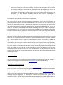
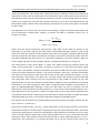
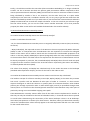
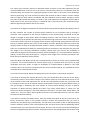
CONEFOR 2.6 User manual (Saura & Torné, April 2012)
Quantifying the importance of habitat patches and links for maintaining or enhancing
landscape connectivity through spatial graphs and habitat availability (reachability) metrics
Table of contents
1. What is Conefor? ................................................................................................................................. 1
2. Authors ................................................................................................................................................ 2
3. Scope of this manual ........................................................................................................................... 2
4. Key new features in version 2.6 compared to version 2.2 .................................................................. 2
5. Installation, operating system and computer configuration............................................................... 3
6. Conditions of use ................................................................................................................................. 3
7. Questions or further information........................................................................................................ 3
8. An overview of the new features in the graphical user interface for Conefor 2.6 ............................. 4
9. Calculating node importance values including the fractions of IIC or PC (intra, flux, connector) ....... 5
10. Generalized Betweenness Centrality metrics ................................................................................... 7
11. Calculating only the overall index values for the entire landscape................................................. 10
12. Calculating the Equivalent Connectivity (EC) for the entire landscape (overall index values)........ 11
13. Calculating the importance only for the added nodes .................................................................... 11
14. Calculating link importance values for different modalities (removal, improvement, change) ..... 12
15. Precision of the calculations (high or standard) .............................................................................. 17
16. Other comments related to Conefor 2.6 ......................................................................................... 17
17. GIS extensions ................................................................................................................................. 17
18. Applications ..................................................................................................................................... 18
19. Empirical support ............................................................................................................................ 18
20. References ....................................................................................................................................... 18
1. What is Conefor?
Conefor is a software package that allows quantifying the importance of habitat areas and links for
the maintenance or improvement of landscape connectivity, as well as evaluating the impact of
habitat and land use changes on connectivity. It is conceived as a tool for decision-making support in
conservation and landscape planning, through the identification and prioritization of critical sites for
ecological connectivity.
Conefor includes new functional connectivity indices (integral index of connectivity (IIC), probability
of connectivity (PC)) that have been shown to present an improved performance compared to other
existing indices and to be particularly suited for landscape conservation planning and change
monitoring applications (Pascual-Hortal and Saura 2006, Saura and Pascual-Hortal 2007, Saura and
Rubio 2010, Saura et al. 2011a). These indices are based on spatial graphs and on the concept of
measuring habitat availability (reachability) at the landscape scale. This concept consists in
Conefor 2.6 user manual
considering a habitat patch itself as a space where connectivity occurs, integrating the connected
resources existing within the patches (intrapatch connectivity) with the resources made available by
(reachable through) the connections with other habitat patches in the landscape (interpatch
connectivity). In this way, connectivity is conceived (and measured) as that property of the landscape
that determines the amount of reachable habitat in the landscape, no matter if such reachable
habitat comes from big and/or high quality habitat patches themselves (intrapatch connectivity),
from strong connections between different patches (interpatch connectivity) or, more frequently,
from a combination of both.
2. Authors
Conefor 2.6 has been developed by Santiago Saura and Josep Torné at Universidad Politécnica de
Madrid as an evolution of the previous 2.2 version (Saura and Torné 2009). See www.conefor.org for
further details and section 20 for appropriate references. Conefor Sensinode 2.2 (released in June
2007) was developed by the same authors at University of Lleida. Funding for developing Conefor has
been provided by the Spanish Ministry of Science and Innovation through projects AGL2009-07140
and REN2003-01628. Sensinode 1.0 (LandGraphs package) was developed by Dean Urban (Duke
University).
3. Scope of this manual
This user manual only explains those new features that have been implemented in Conefor 2.6 and
were not included in version 2.2. All the other functionalities and the basic functioning and
instructions for this software package are the same as for version 2.2. See the manual of version 2.2
(attached) for the rest of (most of) the information on how to use Conefor. Later on we plan to
produce a single updated manual integrating the contents of these two manuals. Check the Conefor
website (www.conefor.org) for updates. In that website you can also subscribe to an email list that
will automatically notify you of any relevant news regarding Conefor.
4. Key new features in version 2.6 compared to version 2.2

The three fractions of the dPC and dIIC indices (intra, flux, connector) are computed (see
section 9), in addition to the total dPC / dIIC values already provided by version 2.2. This
allows separately evaluating the different ways in which habitat patches can contribute to
habitat connectivity and availability in the landscape, i.e. their different roles as connectivity
providers (Saura and Rubio 2010).

The importance for connectivity of individual links (sensilink) can be computed, in addition to
the importance of nodes (sensinode) that was already provided by version 2.2. Several
sensilink functionalities are included in version 2.6, as described in section 14 (link removal,
link improvement, link change). Given that Conefor is now not just performing analyses
related to the nodes (sensinode) but also to the links (sensilink) in the network, the name of
the software package has been shortened and simplified from “Conefor Sensinode” to
“Conefor” in this version 2.6 and future ones.

The values of the Equivalent Connectivity (EC) corresponding to the IIC and PC metrics (Saura
et al. 2011a, 2011b) are also presented in the results for the overall indices (see section 12).
2
Conefor 2.6 user manual

The values of Betweenness Centrality (BC) metrics can now be calculated and presented as
part of the results in the node importance file. This includes the classical BC metric as defined
by Freeman and, more importantly, the generalized and improved versions BC(IIC) and
BC(PC), which provide more ecological realism to this metric and allow it to match with the
requirements and desirable properties of IIC and PC (see section 10). All these metrics are
integrated in a single analytical framework with the same units of measurement, as
described in detail by Bodin and Saura (2010).
5. Installation, operating system and computer configuration
This new version 2.6 has no particular installation requirements. Simply copy the executable file
(Conefor26.exe) anywhere in your computer and double click the file to run the software (you can
even run the software directly from a USB stick). As for version 2.2, Conefor only runs in computers
with a Windows operating system (any Windows version is fine, including Windows XP, Vista, 7 and
others). It runs both in 32-bit and 64-bit architectures, although the current Conefor compilation is
only using 32 bits (i.e. it cannot make use of more than 4 GB RAM in your computer). In the future
we plan to produce Conefor compilations for 64 bits and also for other operating systems different
from Windows (check the Conefor website for updates and/or for subscribing to the Conefor email
list if you want to be automatically notified of future versions or other relevant news).
Note that in the input files for Conefor (node file and connection file) the point (and not the comma)
should be set as the decimal symbol, and that no symbol should be used as a thousand separator
(e.g. a correct number format is 1235.45, while 1.234,45 or 1235,45 or 1,235.45 or 1.234.45 are
incorrect). Conefor will expect all the numerical values in the input files in accordance with these
specifications, and will write the results in the same format. If any numerical value in the input files is
not written according to this format, an error will occur when trying to run Conefor using those input
files. This means that the regional configuration settings of your computer should be set accordingly
before generating the input files for Conefor through any of the GIS extensions that have been
developed specifically for this purpose (see section 17). Otherwise, the GIS extensions will write the
Conefor input files with the wrong numerical format and these files will not be usable for subsequent
processing in Conefor.
6. Conditions of use
Conefor is freeware and has the same conditions of use as version 2.2. This means that it can be used
with no restrictions for non-commercial purposes with the only condition of citing the software, its
website and the appropriate references (see www.conefor.org and section 20 below).
7. Questions or further information
For any question or further information please visit www.conefor.org, where you can find the most
recent versions of the Conefor software package, the user manuals, GIS extensions, related papers,
an overview of the applications in which Conefor has been applied around the world, empirical
support studies and other relevant information. You can also contact us at [email protected]. The
authors would appreciate hearing about the applications in which Conefor is used, as well as help in
reporting bugs and suggestions for improvement. However, very limited user support will be
provided and only for specific questions regarding this software and the methods implemented in it
3
Conefor 2.6 user manual
that cannot be solved by other means (e.g. by carefully reading the manuals and the different related
papers).
8. An overview of the new features in the graphical user interface for Conefor 2.6
Most of the new features in Conefor 2.6 are located within the red boxes indicated in the image
below. The rest is exactly as in version 2.2. The numbers next to each red box indicate in which
section of this user manual you can find the description of that particular option or functionality. See
also section 12 for an additional new feature not indicated graphically in this image.
10
9
14
11
13
15
4
Conefor 2.6 user manual
9. Calculating the node importance values including the fractions of IIC or PC (intra, flux, connector)
Unless you specify the “only overall index” option (see section 11 below), Conefor will calculate the
importance of every node as the decrease in the connectivity metric value caused by the removal of
that individual node from the landscape (see manual for version 2.2 and related papers for further
details). This includes the intra, flux and connector fractions for IIC or PC as described by Saura and
Rubio (2010); these fractions will be automatically calculated if any of these two metrics is selected
for the analysis.
The importance of a node (or link, see section 14) according to a given connectivity index (metric) M
can be expressed in relative terms (“deltas” in Conefor 2.6, dM) or in absolute terms (“vars” in
Conefor 2.6, varM):
( )
Where M is the overall connectivity index (metric) value when all the nodes are present in the
landscape (i.e. the metric value for the initial, intact, undisturbed landscape) and Mafter is the overall
index value after the removal of that individual node from the landscape. Therefore, dM and varM
quantify respectively the relative and absolute variation in the overall connectivity metric value for
the whole landscape (M) after the loss of a particular node/patch. The same equations apply for
other changes related to the links between patches, as will be described later in section 14.
You should select at least “Show deltas” or “Show vars” before running the software (unless the
option “Only overall index” is activated, see below in section 11). If you select the option “Show
deltas” (this is the default), Conefor will calculate and show the dM values for each node and for
each of the indices selected for analysis. If you select the option “Show vars”, Conefor will calculate
and show the varM values for each node and for each of the indices selected for analysis. You can
also select both “Show deltas” and “Show vars” and then Conefor will calculate and show both dM
and varM values. Note, however, that this may generate a large number of columns in the node
importance file, and that the ranking of habitat patches (nodes) by their contribution to landscape
connectivity is the same according to either dM or varM (since both variables are proportional, as
given by varM=(dM·M)/100). Although in some cases dM values are easier to interpret, this will
depend on the selected indices and user preferences. In some cases, if the landscape/network is very
large, dM values can be very low (it is hard for a single node to have a large relative importance for
connectivity if the network is made up by many thousands of nodes) and hard to handle (eventually
indistinguishable from zero). In these cases varM values might be a preferable option.
The index M can correspond to any of the following connectivity metrics included in Conefor 2.6: NL,
NC, H, LCP, IICnum, F, AWF, PCnum.
Note that in Conefor the IICnum and PCnum values (numerators of the IIC and PC metrics, respectively,
see equations below) are those used for computing the dIIC, dPC, varIIC and varPC values. This makes
unnecessary specifying any AL value for calculating the node importances according to IIC or PC. Even
if the IIC and PC values for a particular AL were used (instead of IICnum or PCnum) to calculate the node
importance values, dIIC and dPC would be exactly the same as those obtained using IICnum or PCnum
respectively. This is because AL is a constant that does not vary by the removal of any node or link
5
Conefor 2.6 user manual
from the landscape. If you wish to obtain the varIIC or varPC values as they would result from using
the IIC and PC values (for a given AL value) you just need to divide the varIIC or varPC values that are
calculated by Conefor 2.6 by AL2.
∑
∑
∑
∑
(
)
∑∑
∑∑
See manual for version 2.2 and the two related papers (Pascual-Hortal and Saura 2006, Saura and
Pascual-Hortal 2007) for further details on these metrics and formulas.
As shown by Saura and Rubio (2010) the importance values for the IIC and PC metrics can be
partitioned in three different fractions (intra, flux, connector) considering the different ways in which
a habitat patch (node) or link can contribute to overall habitat connectivity and availability in the
landscape. Conefor 2.6 will automatically calculate for each node the values of these three fractions
separately whenever IIC and/or PC are selected for analysis. This applies to both the dM and varM
values calculated by Conefor as follows (the total dIIC, varIIC, dPC, and varPC values will also be
presented, in addition to the partitioned fraction values):
The three fractions will be calculated both for the existing nodes that can be lost (standard analysis /
node removal) and for the nodes that may be added in the landscape as a result of habitat
restoration measures (see option “nodes to add” in manual for version 2.2). While a habitat patch
can contribute to connectivity through all these three fractions, links (corridors, connectors) can only
contribute through the connector fraction: see Saura and Rubio (2010) for details.
Baranyi et al. (2011) have shown, through cluster analysis and multidimensional scaling, that the
intra, flux and connector fractions provide a non-redundant and complementary information on the
importance of a patch in a landscape network, and that they capture most of the variability in patch
conservation priorities that would derive from using a much larger set of connectivity metrics (see
figure 5 in that study), perhaps complemented by a centrality metric (see section 10 below).
The only exception for the dM and varM calculations in the node importance file (as explained
above) are the values of the Betweenness Centrality metrics (BC, BC(IIC), BC(PC)): these metrics are
calculated in a different way (see section 10 below), and not according to the formulas shown above
for dM or varM. The Betweenness Centrality metrics included in Conefor 2.6 are calculated for each
node just according to their position in the intact (initial) landscape, and not following a node (patch)
removal procedure as for the rest of the metrics.
6
Conefor 2.6 user manual
Finally, it should be noted that the CCP index (Class Coincidence Probability) is no longer included in
Conefor 2.6. This is because CCP does not present good prioritization abilities compared to other
metrics (see Pascual-Hortal and Saura (2006)) and we intend to avoid an excessive number of metrics
being calculated by Conefor if this is not necessary. On the other hand, CCP it is quite similar
analytically to LCP. Since LCP is included in Conefor 2.6, it is very easy to get the CCP values from the
LCP ones calculated by Conefor 2.6 if you wish to do so; see the formulas in Pascual-Hortal and Saura
(2006) to understand how to make this simple calculation. In the rare case that you still want to get
the CCP values directly, you can use the older version Conefor Sensinode 2.2 for that particular
purpose (this older version will be still available for download in the Conefor website).
10. Generalized Betweenness Centrality metrics
10.1. Which network centrality metrics are calculated by Conefor?
Conefor 2.6 calculates for each node:
- BC, the classical Betweenness Centrality metric as originally defined by Freeman (1977; Sociometry
40: 35–41).
- BC(IIC) and BC(PC), the improved versions of the BC metric that were proposed by Bodin and Saura
(2010) in order to incorporate some considerations that are important to increase the ecological
realism of this metric and to make it match with the characteristics and desirable properties of IIC
and PC. In this way, BC(IIC) and BC(PC) are placed (integrated) within the same analytical framework
as the IIC and PC metrics. All these metrics are expressed in the same units of measurement and can
be directly compared. In particular, the normalized BC(IIC) and BC(PC) values for each node are equal
or higher than the connector fraction of the IIC and PC metrics respectively (see section 10.5 below),
as shown by Bodin and Saura (2010).
The values of BC, BC(IIC), and BC(PC) are calculated only for the nodes that exist in the landscape
(standard node importance analysis), and not for the links or the nodes to add.
10.2. What do the Betweenness Centrality metrics measure and how are they calculated?
The baseline concept for all these centrality metrics (BC, BC(IIC), BC(PC)) is the same: they measure
how much a specific node sits between all other pairs of nodes in a network, i.e. these metrics
capture the degree to which the shortest or optimal paths for movement between other habitat
patches pass through a particular node. A node will be highly central (as quantified through these
metrics) when it is involved in the shortest/optimal movement routes between many other pairs of
patches by serving as an intermediate stepping stone patch.
These Betweenness Centrality metrics differ from all the other metrics implemented in Conefor in
that they can only be calculated at the level of individual nodes, i.e. these BC metrics do not provide
an overall value characterizing the connectivity of the entire landscape. There is no M landscapelevel value (see equations in section 9) for these metrics. Therefore, when you select these centrality
metrics for calculation their values will only appear in the node importance file and not in the results
for the overall index values.
7
Conefor 2.6 user manual
The values of the centrality metrics for individual nodes (as shown in the node importance file) are
calculated differently from the rest of the metrics. The centrality values for an individual node are
obtained taking into account the topological position of that node in the intact (initial) landscape,
without performing any node removal procedure (the formula for dM or varM in section 9 above
does not apply for these metrics). See Bodin and Saura (2010) for further details. Therefore, even if
the values of BC, BC(IIC) and BC(PC) are shown in the node importance file together with the dM or
varM values for the rest of the metrics, it should be kept in mind that they are calculated using a
different approach/procedure than for the others.
10.3. Which is the difference between the classical BC and the generalized BC(IIC) and BC(PC) metrics?
BC only considers the number of shortest paths between all pair of patches that go through a
particular node, regardless of the area (or attributes) of the patches being connected and of the
length or strength of those paths. BC(IIC) and BC(PC), however, take into account the area (or any
other attribute) of the patches that are being connected through a particular node, considering more
central those nodes that serve as stepping stones between large and high quality patches than those
that sit in between patches with scarce or poor habitat resources. BC(IIC) also takes into account the
length (number of links) of the paths between patches in which a particular node is involved; longer
paths are considered less feasible for conducting effective movements, and therefore they are given
less weight in the centrality calculations. Similarly, BC(PC) takes into account the probability of
movement through a particular path (maximum product probability p*ij, see Pascual-Hortal and Saura
(2007)), so that those paths with higher p*ij are given more weight in the centrality calculations. See
Bodin and Saura (2010) for further details.
Note that BC(IIC) and BC(PC) are the most computationally intensive of all the metrics implemented
in Conefor. You should therefore be cautious when trying to calculate these two metrics in large
landscapes with many nodes. It might be unfeasible to compute BC(IIC) or BC(PC) in very large
networks due to the excessive computational time that would be required. The standard BC metric
can however be calculated much faster.
10.4. How to select the BC, BC(IIC) and BC(PC) metrics for calculation in the Conefor interface?
If you wish to calculate the classical BC metric, then you should select BC in the box for the binary
connectivity indices in the Conefor interface. The resultant values for each node will be shown in one
of the columns of the node importance file. The BC value calculated by Conefor for a particular node
k correspond to the sum of all separate shortest paths between all pairs of patches (different from k)
that go through k, divided by the total number of shortest paths between all pairs of patches
(equation 5 in Bodin and Saura (2010)). No matter if you select “Show deltas” or “Show vars” the
same result for BC will appear in the node importance file (even if you select both “Show deltas” and
“Show vars”, only one column will be produced for BC in the node importance file, with the values
calculated as described above).
If you wish to calculate the BC(IIC) metric, then you should select both BC and IIC in the box for the
binary connectivity indices in the Conefor interface. Conefor will understand that you want to
calculate not only BC and IIC, but also BC(IIC). This will result in the values for BC, IIC and BC(IIC) being
shown in different columns in the node importance file. The three metrics (BC, IIC and BC(IIC)) will be
calculated even if you are interested only in BC(IIC), but this is not of much concern because BC(IIC) is
the most computationally intensive metric among these three. Calculating BC(IIC) will consume most
8
Conefor 2.6 user manual
of the total processing time. On the other hand, some of the calculations performed to get the BC
and IIC values are also needed to obtain the results for BC(IIC). If you wish to calculate BC and IIC but
not BC(IIC) then you should run Conefor two times, one with only BC selected and the other with only
IIC selected.
If you wish to calculate the BC(PC) metric, then you should select both BC in the box for the binary
indices and PC in the box for the probabilistic indices. Conefor will understand that you want to
calculate not only BC and PC, but also BC(PC). This will result in the values for BC, PC and BC(PC) being
shown in different columns in the node importance file. The three metrics (BC, PC and BC(PC)) will be
calculated even if you are interested only in BC(PC), but this is not of much concern because BC(PC) is
the most computationally intensive metric among these three. Calculating BC(PC) will consume most
of the total processing time. On the other hand, some of the calculations performed to get the BC
and PC values are also needed to obtain the results for BC(PC). Note that if your input connection file
is a distance file, when selecting BC and PC you will need to provide a distance threshold that will be
used for calculating BC (as for any other binary connectivity metric) and a pair of probability-distance
values that will be used for calculating PC and BC(PC). The distance threshold value specified in the
box for the binary indices does not affect at all the calculations for BC(PC), which are just based on
the probability-distance values specified for the probabilistic indices. In the same way, the
calculations for BC are not at all affected by the probability-distance values that are specified for the
probabilistic indices. The same applies if your input connection file is a probability file. In this case a
probability threshold will be requested for calculating BC but this will not affect at all the calculations
for PC or BC(PC), which will run using directly the probability values in the connection file without
requesting any additional distance or probability value in the probabilistic indices box. See the
manual for version 2.2 if you are not familiar with these latter considerations. If you wish to calculate
BC and PC but not BC(PC) then you should run Conefor two times, one with only BC selected and the
other with only PC selected.
10.5. How do the generalized Betweenness Centrality metrics relate to the connector fraction of IIC
and PC? How should this relationship be interpreted?
If you select “Show deltas”, the BC(IIC) and BC(PC) values will be scaled in the same way as for dIIC
and dPC (dIICconnector and dPCconnector), and the resultant values for each node will be shown in
two columns with names dBC(IIC) and dBC(PC). In this case, dBC(IIC) ≥ dIICconnector and dBC(PC) ≥
dPCconnector. Note, however, that the names dBC(IIC) and dBC(PC) just indicate that the values are
directly comparable with those for dIICconnector and dPCconnector. It does not mean that the
dBC(IIC) and dBC(PC) values are calculated as the relative variation in any connectivity metric value
following any patch removal procedure. See Bodin and Saura (2010) for details and equations.
If you select “Show vars”, the BC(IIC) and BC(PC) values will be scaled in the same way as for varIIC
and varPC (varIICconnector and varPCconnector), and the resultant values for each node will be
shown in two columns with names varBC(IIC) and varBC(PC). In this case varBC(IIC) ≥ varIICconnector
and varBC(PC) ≥ varPCconnector. Note however that the names varBC(IIC) and varBC(PC) just indicate
that the values are directly comparable with those for varIICconnector and varPCconnector. It does
not mean that dBC(IIC) and dBC(PC) values are calculated as the absolute variation in any
connectivity metric value following any patch removal procedure. If you select both “Show deltas”
and “Show vars”, then the values for BC(IIC) and BC(PC) in the node importance file will be
respectively scaled and shown both as dBC(IIC) and dBC(PC) and as varBC(IIC) and varBC(PC).
9
Conefor 2.6 user manual
The centrality metrics are calculated in the intact landscape and do not consider how the flows might
change as a consequence of losing a particular patch. Unlike the connector fraction of the IIC and PC
metrics, they do not deliver estimates of the impacts of a patch removal in terms of connectivity loss.
The pairs of values dBC(IIC) and dIICconnector for a given node k should be interpreted in the
following way (exactly the same applies to the pairs of values varBC(IIC) and varIICconnector, dBC(PC)
and dPCconnector, and varBC(PC) and varPCconnector): dBC(IIC) quantifies the amount of fluxes that
are expected to go through k in the intact landscape (the undisturbed landscape in which no habitat
patch has been lost), because k is part of the best (shortest or most probable) paths between other
habitat patches. However, dBC(IIC) does not quantify how much the connectivity between other
habitat areas depends on the presence of k in the landscape, i.e. it does not measure how
irreplaceable k is as a connecting element between other habitat areas. This latter aspect is what is
measured by dIICconnector. It might happen that even if k is considerably involved in the fluxes
occurring in the current landscape (high dBC(IIC)), the loss of k does not have a large impact in the
connectivity between the other habitat areas (low dIICconnector, much smaller than dB(IIC)),
because the connectivity that was provided by k as a connecting element or stepping stone has been
largely or fully compensated by other patches and alternative paths available for movement in the
landscape. If, however, k is the only element sustaining the connectivity between other habitat
areas, and there are no other alternative patches or paths available to compensate for its loss, the
removal of k will have a large impact in the connectivity of the remnant network (dIICconnector will
be in this case as high as dBC(IIC)). Therefore, these metrics capture how much of the current
stepping stone (connecting) role played by a particular patch in the intact landscape (dBC(IIC)) is lost
when that patch is removed from the landscape (dIICconnector). See Bodin and Saura (2010) for
further details on these metrics and their ecological interpretation.
BC(IIC) or BC(PC) can be considered as a “fourth fraction” of the IIC or PC metrics, being measured
with the same units and within the same analytical framework than the intra, flux and connector
fractions (a common currency for connectivity). These four metrics/fractions provide a multifaceted,
complete and non-redundant view of the different ways in which habitat patches can be important
as connectivity providers, as supported both in analytical grounds (Saura and Rubio 2010, Bodin and
Saura 2010) and by statistical assessments on their practical outcomes as compared to a wider set of
connectivity metrics, as shown by figure 5 and the rest of the content in Baranyi et al. (2011).
11. Calculating only the overall index values for the entire landscape
The option “Only overall index” (first option in the “Mode” box) should be selected when you are
only interested in obtaining the overall index values for the whole landscape (M) and not in the
importance values for each individual node or link (dM or varM).
This option allows the user to save a lot of processing time when the interest is only in the M value.
This is because the overall index value M is much faster to compute than the dM or varM values for
every node. Obtaining M requires just one calculation of the metric value, while obtaining dM or
varM requires n additional calculations of the metric value (one for each node), where n is the total
number of nodes in the landscape. Much more calculations of the metric value (in general n·(n-1)/2)
are required for obtaining dM or varM if any of the link importance analysis options if selected (see
section 14 below).
Obviously, if the “Only overall index” is selected the dM or varM values (node or link importance
files) will not be calculated. As stated in the previous section, the results for the overall index values
10
Conefor 2.6 user manual
will not contain any value for the Betweenness Centrality metrics even if these have been selected
for calculation.
12. Calculating the Equivalent Connectivity (EC) for the entire landscape (overall index values)
If you compute IIC or PC and go for the “Results -> Overall index values”, you will notice that in this
new version, in addition to the IIC or PC (or IICnum or PCnum) values already provided by version 2.2,
the results also include the EC (Equivalent Connectivity) values for these two indices: EC(IIC) and
EC(PC). This corresponds to the Equivalent Connected Area (ECA) index as described in Saura et al.
(2011a, 2011b), where the patch habitat area was used as the node attribute. ECA(IIC) and ECA(PC)
are defined as the size of a single habitat patch (maximally connected) that would provide the same
value of the IIC and PC metric (respectively) as the actual habitat pattern in the landscape. In a more
general case in which the attributes of the nodes might correspond to some other characteristic
different from just habitat area (e.g., habitat quality, population size, etc.) this index is better
renamed as EC (Equivalent Connectivity). Therefore this more general name (EC) is the one used in
Conefor 2.6.
EC or ECA is just computed as the square root of the numerator of the IIC and PC indices (IICnum and
PCnum), yielding EC(IIC) and EC(PC), respectively. Although Saura et al. (2011a, 2011b) only used
EC/ECA for the PC index (EC(PC)), the same approach and advantages (see below) apply for IIC
(EC(IIC)). Both EC(PC) and EC(IIC) are calculated by this new version. You just need to select IIC or PC
for analysis, and the results for the overall index values will also show the EC(IIC) and EC(PC) values,
respectively.
EC(IIC) and EC(PC) maintain all the desirable properties and good prioritization abilities of IIC and PC
but have the following advantages (as an overall index value) compared to IIC and PC: (a) they avoid
the very low metric values that might be obtained for IIC and PC when the amount of habitat is very
small compared to the total extent of the analyzed landscape, since EC(IIC) and EC(PC) will not be
smaller than the largest attribute (e.g. habitat area) for the patches in the landscape; (b) EC(IIC) and
EC(PC) have the same units as the attributes of the nodes, which facilitates the interpretation and
understanding of the resultant values; (c) EC(IIC) and EC(PC) avoid the need of specifying any AL
value, as is needed for IIC and PC, which in some cases might not be straightforward and might be to
some degree arbitrary; and, more importantly (d) the relative variation in EC(IIC) or EC(PC) after a
particular spatial change (or set of changes) in the landscape can be directly compared with the
variation in the total amount of habitat area in the landscape (or any other considered node
attribute) after the same change, with an easy interpretation and additional insights that can be
gained from that comparison (Saura et al. 2011a, 2011b). This latter property makes EC(IIC) and
EC(PC) quite convenient for quantifying changes in landscape connectivity and comparing them with
the changes in the amount of habitat in the landscape, as described in Saura et al. (2011a, 2011b).
See figure 1 in Saura et al. (2011a) and figure 1 in Saura et al. (2011b).
13. Calculating the importance only for the added nodes
When the option “Only added nodes” is selected, Conefor will make the calculations of the dM or
varM values only for the potential nodes that may be added in the landscape (as a result of potential
habitat restoration actions that may improve connectivity), and not for the nodes that already exist
11
Conefor 2.6 user manual
in it (the impact on connectivity of their potential loss will not be evaluated). Selecting “Only nodes
to add” will also deactivate any of the options for link importance analysis.
This option (“Only added nodes”) is active only when the option “There are nodes to add” has been
previously selected in the box for the node file. When “There are nodes to add” has been selected
Conefor will expect a node file with three columns (see section 4.2 in the manual for version 2.2) and
will in general calculate (a) the dM or varM values representing the connectivity loss that would be
caused by the removal of each of the nodes that exist in the current/initial landscape, and (b) the dM
or varM values representing the connectivity improvement that would occur thanks to the addition
of new nodes in the landscape as resulting from habitat restoration measures (see manual for
version 2.2 for details). If the option “Only added nodes” is selected Conefor will just calculate (b), i.e.
it will only evaluate how much each of the new potential habitat areas (nodes to add) would
contribute to improve connectivity if they were added in the landscape. Since, in general, the
number of candidate nodes to be added in the landscape (b) is much smaller than all the
nodes/patches that exist in it (a), this option can save a lot of processing time by just calculating the
dM or varM values for the nodes to add and not for the existing nodes. Note that BC, BC(IIC) and
BC(PC) metrics are not calculated for the nodes to add; the values for these metrics will be equal to
zero in the node importance file, but this just means that they have not been calculated.
14. Calculating link importance values for different modalities (removal, improvement, change)
14.1. What does “link importance” mean and which results are obtained through this analysis?
Conefor 2.6 includes the possibility of calculating the contribution of individual links to maintain or
improve overall landscape connectivity. This goes beyond the capabilities of previous Conefor
versions, in which such type of analysis was possible only for nodes and not for links. Some recent
studies have benefited from this new functionality in Conefor (see the section on applications at the
Conefor website for the full references): Gurrutxaga et al. (2011; Landscape and Urban Planning 101:
310-320), Saura et al. (2011; Forest Ecology and Management 262: 150-160), Carranza et al. (2012;
Landscape Ecology 27: 281-290), Rubio et al. (in press; Forest Systems).
The importance of a link for maintaining or improving connectivity is calculated in the same way as
for the nodes (see section 9), i.e. as the relative (dM) or absolute (varM) variation in the value of a
given connectivity metric M after a certain change affecting one of the links in the landscape.
Note that links can only contribute to habitat connectivity and availability (as measured by IIC and
PC) through the connector fraction. Since a link is defined as a connecting element that contains no
habitat area, a link cannot contribute through the intra fraction. For the same reason, a link cannot
be the final/permanent destination for any dispersal flux. Therefore both the intra and the flux
fractions will be by definition equal to zero for any link in the landscape. If a connecting element
contains some habitat area, this should be modeled as a node in the graph, and its value as a
connecting element or stepping stone will be anyway quantified through the connector fraction of
the IIC or PC metrics, together with its potential contribution through the intra and flux fractions. The
connector values for links can be directly compared with the connector values for nodes. See Saura
and Rubio (2010) for details. In summary, even when Conefor will express the results of the link
importance values as dIIC, varIIC, dPC and varPC (depending on the metric and type of result selected
in the Conefor interface), the user should be aware that for links these values correspond in fact
12
Conefor 2.6 user manual
exclusively to the connector fraction, that is, they correspond to dIICconnector, varIICconnector,
dPCconnector and varPCconnector respectively, even if this is not written explicitly in the link
importance result files.
Note also that the link importance analysis can be much more time consuming than the node
importance analysis. While a node importance analysis will require n+1 calculations of the metric
value (M) in a graph with n nodes, a link importance analysis in the same graph will require n(n-1)/2 +
1 calculations of the metric value (since n(n-1)/2 is the number of links in an undirected complete
graph with n nodes). This can be considerably slow and even unfeasible in large networks, especially
for computationally intensive metrics like PC. Users should keep this in mind when trying to analyze
large datasets through this new functionality in Conefor 2.6. Some options that might allow users to
reduce the number of calculations and the required processing time are being evaluated and might
be included in a future version of this software package (check www.conefor.org for updates or
subscribe there to the Conefor email list if desired).
The link importance analysis in Conefor 2.6 does not include the calculation of any of the
Betweenness Centrality metrics (see section 10), which are only calculated for individual nodes.
The link importance analysis can be performed under the following three different modalities that
can be selected in the “Link importance” box in the Conefor interface: link removal, link
improvement and link change.
14.2. Link removal: the impact of losing an existing link.
When the “Link removal” option is selected, Conefor will remove one by one each of the links
existing in the landscape network (individual link removal, only one link removed at the same time)
and calculate the impact of that link loss on landscape connectivity according to dM or varM (where
M can be any of the metrics implemented in Conefor except the Betweenness Centrality metrics,
although IIC and PC are the ones recommended for this and other types of analyses). This will
produce a dM or varM value for all the pairs of patches/nodes in the landscape, each link being
represented by the IDs of the nodes it connects.
In the binary connection model (the one that applies for IIC) those patches that are not linked in the
initial/intact landscape will surely have dM=0 and varM=0 (there is obviously no impact in the
potential loss of a link between two patches if such link does not actually exist in the initial
landscape). For those pairs of patches that do have a link in the initial landscape, Conefor will
recalculate the index value after removing that link (Mafter, see section 9), which will result in a dM
and varM that might be (although not necessarily) higher than zero.
For the same reason as above, in the probabilistic connection model (the one that applies for PC),
those pairs of patches that have no direct connection between them (pij=0) will surely have dM=0
and varM=0. For the rest of the cases (pairs of patches with pij>0), Conefor will change the pij value
for each pair of patches from its initial value in the intact landscape to pij=0, and recalculate the value
of M after that change (Mafter), which will result in a dM and varM that might be higher than zero.
In the binary connection model all the link losses are comparable in the magnitude of change they
represent (a link that existed in the initial landscape is removed completely to evaluate the impact of
its loss). However, in the probabilistic model the initial value of pij for each link in the initial landscape
might be very different among the different links. This introduces some complication when trying to
13
Conefor 2.6 user manual
directly compare the dM or varM values resulting from this analysis for the different links in the
probabilistic model, since the actual magnitude of change in the strength or probability of use of
each link (as characterized by pij) might be quite different for each link. For example, it is not the
same obtaining dM=10% for a link which had pij=0.01 in the initial landscape than obtaining the same
dM=10% for another link that had a pij=0.9 in the initial landscape. This has to be taken into account
when trying to interpret and summarize the results of this link removal analysis for the probabilistic
connection model.
If the “Link removal” option is selected, there is the possibility to use the “Reduce calculations”
option (see the box for the link importance options in the Conefor interface). Such “Reduce
calculations” option allows specifying a maximum distance (if the connection file is a distance file) or
a minimum probability (if the connection file is a probability file) so that the calculations are
performed only for the pairs of patches (links) with a distance not larger than the specified maximum
or with a probability pij not smaller than the specified minimum. Note that in this case the rest of the
links (those weak links with large distances or small probabilities) will get dM=0 and varM=0 because
they have not been evaluated in the analysis; this does not mean that the results would be
necessarily zero if the “Reduce calculations” option would not have been selected.
14.3. Link improvement: the potential benefits of strengthening connections between habitat patches
When the option “Link improvement” is selected, Conefor will perform quite the opposite analysis to
that of the “Link removal” option.
In the binary connection model (the one that applies for IIC), Conefor will add one link (only one at a
time) to each of those pairs of patches that are not directly linked in the initial landscape, and will
recalculate the M value after that change/addition (Mafter). This may result in a connectivity gain as
measured by metric M, case in which dM<0 and varM<0. Note that the relative and absolute
variations of the IIC and PC metrics (dM and varM) will have negative values in this case because
Mafter is higher than M (see the formula for dM and varM in section 9), but in fact these negative
values mean that connectivity has improved. Obviously, for those pairs of patches that were already
linked in the initial landscape, the connectivity cannot increase by adding a link that in fact already
existed, and therefore dM=0 and varM=0.
In the probabilistic connection model (the one that applies for PC), Conefor will calculate the
potential (positive) impacts of improving as much as possible the direct connection (link) between
each pair of patches (only one at a time). In this probabilistic model this translates in assigning a pij=1
to each pair of patches, which means that the strength or frequency of use of the direct connection
between i and j (as quantified by pij) will be improved for all the pairs of patches except for those that
already had pij =1 in the initial landscape. For those pairs of patches with pij=1 in the initial landscape
the result will necessarily be dM=0 and varM=0. For the rest, the increase in the pij value for each link
may result (although not necessarily) in an improvement in connectivity as quantified by dM or varM
(as said above, such improvement will correspond to negative dM and varM values).
In the binary connection model all the link gains are comparable in the magnitude of change they
represent (a link that did not exist in the initial landscape is added to evaluate the potential benefits
of its creation or restoration). However, in the probabilistic model the initial value of pij for each link
in the initial landscape might be very variable among the different links. This introduces some
complication when trying to directly compare the dM or varM values resulting from this analysis for
14
Conefor 2.6 user manual
the different links in the probabilistic model, since the actual magnitude of change in the strength or
probability of use of each link (as characterized by pij) might be quite different for each link. For
example, it is not the same obtaining dM=10% for a link which had pij=0.01 in the initial landscape
than obtaining the same dM=10% for another link that had a pij=0.9 in the initial landscape. This has
to be taken into account when trying to interpret and summarize the results of this link improvement
analysis for the probabilistic connection model.
Note that not all the link changes that are set by the “Link improvement” option can be considered
realistic. For example, if the dispersal abilities of your analyzed species are in the range of a few
hundred meters, it would be certainly unrealistic to consider that pij can improve up to 1 for two
patches that are separated by hundreds of kilometers, no matter how much increase in the
permeability or hospitability of the landscape matrix you may be able to achieve. However, the link
improvement option will evaluate such hypothetical (and unrealistic) improvement in the strength or
feasibility of use of that link (as characterized by pij) in the same way as for all the other pairs of
patches. The resultant dM or varM values may be therefore only feasible to obtain in reality for a
small subset of the total number of links (direct connections) in your graph. To overcome this issue
and perform a more fine-tuned and detailed analysis related to the potential changes in the links in
your landscape you might consider instead the “Link change” modality that is described in the next
subsection.
Finally, in the same way as described above for the “Link removal” analysis, if the “Link
improvement” option is selected, there is also the possibility to use the “Reduce calculations” option
(see the box for the link importance options in the Conefor interface). Such “Reduce calculations”
option allows specifying a maximum distance (if the connection file is a distance file) or a minimum
probability (if the connection file is a probability file) so that the calculations are performed only for
the pairs of patches (links) with a distance not larger than the specified maximum or with a
probability pij not smaller than the specified minimum. Note that in this case the rest of the links
(those weak links with large distances or small probabilities) will get dM=0 and varM=0 because they
have not been evaluated in the analysis; this does not mean that they would be zero if the “Reduce
calculations” option would not have been selected.
14.4. Link change: how user-defined changes in the links translate in connectivity gains or losses
This is the most powerful and flexible modality for link importance analysis. It however requires
additional input information to be provided by the user compared to the link removal and link
improvement options.
If the option “Link change” is selected, Conefor will require the connection file to have four columns
instead of three as in the usual case (in fact, this is the only processing option in which the
connection file needs to have four instead of three columns). The first three columns are the same as
in any connection file for Conefor: ID of node i, ID of node j, and a value (typically some form of
distance or a direct dispersal probability pij) characterizing the connection between nodes i and j in
the initial landscape (see manual for version 2.2 for further details). The fourth column required by
the “Link change” option will also contain a value characterizing the connection between nodes i and
j, but this value will correspond to the new distance or direct dispersal probability between nodes i
and j that would result in a given change scenario. This value in the fourth column will be in general
different than the value in the third column; a smaller distance or a larger probability in the fourth
than in the third column will correspond to the case in which the quality or strength of the link
15
Conefor 2.6 user manual
between two patches increases in a given change scenario; and a higher distance or smaller
probability in the fourth than in the third column will mean that the connection between those two
patches gets weaker. All types of combinations and different types of changes are possible for each
of the links in a given landscape and “Link change” analysis. For example, some connections may be
improved, some others may decrease its quality or even disappear completely, and some other links
may suffer no change at all in the same analysis, depending on the particular values for each link that
are specified in the third and fourth columns of the connection file. Obviously, for those links with
the same values in the third and fourth column of the connection file the result will necessarily be
dM=0 and varM=0, since that would mean that no change is foreseen (evaluated) for that particular
link. It is also possible to use a link file as the connection file for the “Link change” option, although in
this case only binary metrics such as IIC can be calculated, with the only possible changes for
individual links being the complete disappearance of an existing link or the addition of a link (direct
connection) between patches that did not exist in the initial landscape. Therefore, in this case, both
the third and the fourth column of the connection file can only contain either 0 or 1 for each pair of
patches, indicating if a link exists (1) or not (0) between those patches in the initial landscape (third
column) and if it will be lost, gained or will remain unchanged in a given scenario (as specified in the
forth column of the connection file).
In the “Link change” analysis Conefor will replace the value for a particular pair of patches in the
third column of the connection file by the value in the fourth column of that file, which in general
might either make a link appear or disappear (binary connection model) or change the pij value that
is associated to that link (probabilistic connection model). Conefor will recalculate the network
connectivity (as evaluated by the value of Mafter for the entire landscape) after that change, and will
report the resultant dM or varM value. This change will be done only for individual links (one at a
time), so that dM or varM values correspond to the connectivity change (either gain or loss) that
would result from implementing that change in a given link while all the others remain unchanged.
As said above for the other modalities of link importance analysis, the connectivity losses as
measured by IIC or PC will correspond to positive dM and varM values, while connectivity gains will
correspond to negative dM or varM values (see formulas in section 9 for these variables).
The changes evaluated through this option might correspond to an increased effective distance or
resistance due to the intensification of a certain part of the landscape matrix (e.g. the development
of a highway or other type of barrier), to an increase in the permeability or hospitability of the
landscape matrix, or to many other types and intensities of change that may be of interest in
particular case studies and regions in accordance with the objectives of a given connectivity analysis.
Note that in fact the “Link removal” and “Link improvement” options are just particular cases of the
“Link change” modality, but with the former two not requiring to include a fourth column in the
connection file (since they assume that all the evaluated links change exactly to the same state,
which is the disappearance of a link or the unlimited improvement of the quality of a link,
respectively). If you use the “Link change” option and your connection file is for example a distance
file, then if you set the fourth column all to zero values, the “Link change” result will be the same as
that for “Link improvement”. If in the same case you set all the values in the fourth column to
arbitrarily large (infinite) values, then the “Link change” result will be the same as for “Link removal”.
If your connection file is either a probabilities file or a link file, then setting all the values in the fourth
column to zero will provide the same results as in the “Link removal” option, while setting all the
values in the fourth column to one will provide the same results as in the “Link improvement” option.
16
Conefor 2.6 user manual
The “Reduce calculations” option does not apply to the “Link change” analysis (it only affects the
“Link removal” and “Link improvement” modalities).
15. Precision of the calculations (high or standard)
The precision in the calculation of the values that Conefor will produce as an output can be set to
either “High” or “Standard”.
In version 2.2 the standard precision was used (no choice was possible in that version) and that was
fine for the applications for which that version was intended to be used. However, when the three
fractions (intra, flux, connector) of IIC and PC are to be computed separately (as provided in this new
version) a higher precision is advisable to provide more accurate results for these three fractions,
especially in large graphs / habitat networks. Therefore the high precision is the default in this new
version.
The high precision will consume more RAM and require a slightly higher processing time than the
standard precision (depending on the size of the network and on the computer characteristics), but
this should not make a significant difference for most of the users (unless your network is so large
and/or your RAM memory so small that you are forced to use the standard precision to make the
processing feasible). In summary, you can change to the standard precision only if either you do not
need the separated fraction values (i.e. you will just use the overall index value M or the total dM or
varM value for each node) or if your computer is not able to process the graph with the more
demanding high-precision mode.
16. Other comments related to Conefor 2.6
The option to save DBF files is disabled in this new version, but you may easily convert the text files
(the output format for the results in Conefor) into DBF format with any other external software if
needed. Almost any software package (GIS, spreadsheet, statistical, etc.) is able to directly read the
text files as produced by Conefor. ArcGIS is able to directly open and work with them as tables, as
long as each column has an appropriate header (some of the files produced by Conefor already
include these headers for each column; for the others you can easily add them in a new (first) line of
text with any text editor). In the particular case of ArcGIS, some characters like parenthesis are not
admitted in the names of the column headers; this means that you should manually change the
headers for the BC(IIC) or BC(PC) metrics in the node importance file (e.g. to BC_IIC and BC_PC), if
this metrics have been selected for computation, before you can open this result file in ArcGIS.
Finally, in the “PC->More->PC setup” window in the Conefor interface, you may notice that a new
option “Alternative calculation mode” has been added. This is however an implementation in
progress that should be handled with much care. We recommend users not to perform any
calculations of the PC metric with this option activated.
17. GIS extensions
Several GIS extensions have been developed specifically for Conefor. These extensions allow
generating from a spatial layer (in either vector or raster format) the files required as an input to
perform the connectivity analyses in Conefor. These extensions generate these input files (node file
and connection file) directly in the exact format required by Conefor; therefore, these files can be
17
Conefor 2.6 user manual
used as they result from the GIS extensions with no other changes or intermediate processing steps.
The extensions allow for batch processing of multiple files/layers. You can find more details about
these extensions (including the web pages from where they can be downloaded) at
http://www.conefor.org/gisextensions.html.
18. Applications
Conefor and the new IIC and PC metrics have been used in a wide variety of conservation and
management plans, scientific studies, and official reports on biodiversity indicators by the European
Commission and the European Environmental Agency, among other connectivity-related
applications. Such applications have been reported in numerous studies comprising different types of
species and ecosystems and a large number of countries, from China to the USA and from Brazil to
Finland. You can get more details on these applications (and perhaps inspiration on the way you can
use Conefor for the purposes of your own case study) from the references listed in
http://www.conefor.org/applications.html, and in the map of Conefor applications available here.
19. Empirical support
Several studies have evaluated and demonstrated the ability of the new habitat availability
(reachability) metrics implemented in Conefor (IIC, PC, etc.) to explain or predict ecological processes
related to landscape connectivity, including species distributions, colonization events or genetic
diversity patterns at the landscape scale. Most of these studies have been performed by other
research groups and institutions different from the one that developed Conefor and the metrics
there implemented, which provides an independent assessment and empirical support to these
quantitative developments and metrics. Some of these studies have evaluated the ability of IIC or PC
to explain ecological processes and have compared it with the performance of other existing
connectivity metrics. When this has been done, IIC or PC have been shown to outperform the other
analyzed connectivity metrics by presenting a stronger relationship with the analyzed ecological
processes and empirical data. You can find more details on this empirical support and validation at
http://www.conefor.org/empirical.html.
20. References
For the IIC and PC metrics:
-
-
Pascual-Hortal, L. & Saura, S. 2006. Comparison and development of new graph-based
landscape connectivity indices: towards the priorization of habitat patches and corridors for
conservation. Landscape Ecology 21 (7): 959-967. Download
Saura, S. & Pascual-Hortal, L. 2007. A new habitat availability index to integrate connectivity
in landscape conservation planning: comparison with existing indices and application to a
case study. Landscape and Urban Planning 83 (2-3): 91-103. Download
For the three fractions of the PC or IIC metrics (intra, flux, connector):
-
Saura, S. & Rubio, L. 2010. A common currency for the different ways in which patches and
links can contribute to habitat availability and connectivity in the landscape. Ecography 33:
523-537. Download
18
Conefor 2.6 user manual
For the Equivalent Connectivity (EC) or Equivalent Connected Area (ECA) index and its use for
monitoring changes in landscape connectivity:
-
-
Saura, S., Estreguil, C., Mouton, C. & Rodríguez-Freire, M. 2011a. Network analysis to assess
landscape connectivity trends: application to European forests (1990-2000). Ecological
Indicators 11: 407-416. Download
Saura, S., González-Ávila, S. & Elena-Rosselló, R. 2011b. Evaluación de los cambios en la
conectividad de los bosques: el índice del área conexa equivalente y su aplicación a los
bosques de Castilla y León. Montes, Revista de Ámbito Forestal 106: 15-21 (only available in
Spanish). Download 1 (short version as published on paper). Download 2 (expanded version
as available only online at http://www.revistamontes.net/).
For the generalized Betweenness Centrality metrics BC(IIC) and BC(PC):
-
Bodin, Ö. & Saura, S. 2010. Ranking individual habitat patches as connectivity providers:
integrating network analysis and patch removal experiments. Ecological Modelling 221:
2393-2405. Download
For the complete, non-redundant and multifaceted view provided by the IIC or PC-related fractions
or metrics:
-
Baranyi, G., Saura, S., Podani, J. & Jordán, F. 2011. Contribution of habitat patches to
network connectivity: redundancy and uniqueness of topological indices. Ecological
Indicators 11: 1301-1310. Download
For the software:
-
Saura, S. & Torné, J. 2009. Conefor Sensinode 2.2: a software package for quantifying the
importance of habitat patches for landscape connectivity. Environmental Modelling &
Software 24: 135-139. Download
We prefer any of the references above for citing the Conefor software package or the metrics and
methods implemented in it. If however, for some reason, you need to cite this manual for any
content that is not available in the previous papers, please use the following reference:
-
Saura, S. & Torné, J. 2012. Conefor 2.6 user manual (April 2012). Universidad Politécnica de
Madrid. Available at www.conefor.org.
19