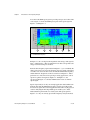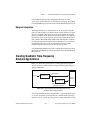
1
LabVIEW
TM
Advanced Signal Processing Toolkit
Time Frequency Analysis Tools User Manual
Time Frequency Analysis Tools User Manual
August 2005
371552A-01
Support
Worldwide Technical Support and Product Information
ni.com
National Instruments Corporate Headquarters
11500 North Mopac Expressway Austin, Texas 78759-3504
USA Tel: 512 683 0100
Worldwide Offices
Australia 1800 300 800, Austria 43 0 662 45 79 90 0, Belgium 32 0 2 757 00 20, Brazil 55 11 3262 3599,
Canada 800 433 3488, China 86 21 6555 7838, Czech Republic 420 224 235 774, Denmark 45 45 76 26 00,
Finland 385 0 9 725 725 11, France 33 0 1 48 14 24 24, Germany 49 0 89 741 31 30, India 91 80 51190000,
Israel 972 0 3 6393737, Italy 39 02 413091, Japan 81 3 5472 2970, Korea 82 02 3451 3400,
Lebanon 961 0 1 33 28 28, Malaysia 1800 887710, Mexico 01 800 010 0793, Netherlands 31 0 348 433 466,
New Zealand 0800 553 322, Norway 47 0 66 90 76 60, Poland 48 22 3390150, Portugal 351 210 311 210,
Russia 7 095 783 68 51, Singapore 1800 226 5886, Slovenia 386 3 425 4200, South Africa 27 0 11 805 8197,
Spain 34 91 640 0085, Sweden 46 0 8 587 895 00, Switzerland 41 56 200 51 51, Taiwan 886 02 2377 2222,
Thailand 662 278 6777, United Kingdom 44 0 1635 523545
For further support information, refer to the Technical Support and Professional Services appendix. To comment
on National Instruments documentation, refer to the National Instruments Web site at ni.com/info and enter
the info code feedback.
© 2005 National Instruments Corporation. All rights reserved.
Important Information
Warranty
The media on which you receive National Instruments software are warranted not to fail to execute programming instructions, due to defects
in materials and workmanship, for a period of 90 days from date of shipment, as evidenced by receipts or other documentation. National
Instruments will, at its option, repair or replace software media that do not execute programming instructions if National Instruments receives
notice of such defects during the warranty period. National Instruments does not warrant that the operation of the software shall be
uninterrupted or error free.
A Return Material Authorization (RMA) number must be obtained from the factory and clearly marked on the outside of the package before
any equipment will be accepted for warranty work. National Instruments will pay the shipping costs of returning to the owner parts which are
covered by warranty.
National Instruments believes that the information in this document is accurate. The document has been carefully reviewed for technical
accuracy. In the event that technical or typographical errors exist, National Instruments reserves the right to make changes to subsequent
editions of this document without prior notice to holders of this edition. The reader should consult National Instruments if errors are suspected.
In no event shall National Instruments be liable for any damages arising out of or related to this document or the information contained in it.
EXCEPT AS SPECIFIED HEREIN, NATIONAL INSTRUMENTS MAKES NO WARRANTIES, EXPRESS OR IMPLIED, AND SPECIFICALLY DISCLAIMS ANY WARRANTY OF
MERCHANTABILITY OR FITNESS FOR A PARTICULAR PURPOSE. CUSTOMER’S RIGHT TO RECOVER DAMAGES CAUSED BY FAULT OR NEGLIGENCE ON THE PART OF
NATIONAL INSTRUMENTS SHALL BE LIMITED TO THE AMOUNT THERETOFORE PAID BY THE CUSTOMER. NATIONAL INSTRUMENTS WILL NOT BE LIABLE FOR
DAMAGES RESULTING FROM LOSS OF DATA, PROFITS, USE OF PRODUCTS, OR INCIDENTAL OR CONSEQUENTIAL DAMAGES, EVEN IF ADVISED OF THE POSSIBILITY
THEREOF. This limitation of the liability of National Instruments will apply regardless of the form of action, whether in contract or tort, including
negligence. Any action against National Instruments must be brought within one year after the cause of action accrues. National Instruments
shall not be liable for any delay in performance due to causes beyond its reasonable control. The warranty provided herein does not cover
damages, defects, malfunctions, or service failures caused by owner’s failure to follow the National Instruments installation, operation, or
maintenance instructions; owner’s modification of the product; owner’s abuse, misuse, or negligent acts; and power failure or surges, fire,
flood, accident, actions of third parties, or other events outside reasonable control.
Copyright
Under the copyright laws, this publication may not be reproduced or transmitted in any form, electronic or mechanical, including photocopying,
recording, storing in an information retrieval system, or translating, in whole or in part, without the prior written consent of National
Instruments Corporation.
Trademarks
National Instruments, NI, ni.com, and LabVIEW are trademarks of National Instruments Corporation. Refer to the Terms of Use section
on ni.com/legal for more information about National Instruments trademarks.
Other product and company names mentioned herein are trademarks or trade names of their respective companies.
Members of the National Instruments Alliance Partner Program are business entities independent from National Instruments and have no
agency, partnership, or joint-venture relationship with National Instruments.
Patents
For patents covering National Instruments products, refer to the appropriate location: Help»Patents in your software, the patents.txt file
on your CD, or ni.com/patents.
WARNING REGARDING USE OF NATIONAL INSTRUMENTS PRODUCTS
(1) NATIONAL INSTRUMENTS PRODUCTS ARE NOT DESIGNED WITH COMPONENTS AND TESTING FOR A LEVEL OF
RELIABILITY SUITABLE FOR USE IN OR IN CONNECTION WITH SURGICAL IMPLANTS OR AS CRITICAL COMPONENTS IN
ANY LIFE SUPPORT SYSTEMS WHOSE FAILURE TO PERFORM CAN REASONABLY BE EXPECTED TO CAUSE SIGNIFICANT
INJURY TO A HUMAN.
(2) IN ANY APPLICATION, INCLUDING THE ABOVE, RELIABILITY OF OPERATION OF THE SOFTWARE PRODUCTS CAN BE
IMPAIRED BY ADVERSE FACTORS, INCLUDING BUT NOT LIMITED TO FLUCTUATIONS IN ELECTRICAL POWER SUPPLY,
COMPUTER HARDWARE MALFUNCTIONS, COMPUTER OPERATING SYSTEM SOFTWARE FITNESS, FITNESS OF COMPILERS
AND DEVELOPMENT SOFTWARE USED TO DEVELOP AN APPLICATION, INSTALLATION ERRORS, SOFTWARE AND
HARDWARE COMPATIBILITY PROBLEMS, MALFUNCTIONS OR FAILURES OF ELECTRONIC MONITORING OR CONTROL
DEVICES, TRANSIENT FAILURES OF ELECTRONIC SYSTEMS (HARDWARE AND/OR SOFTWARE), UNANTICIPATED USES OR
MISUSES, OR ERRORS ON THE PART OF THE USER OR APPLICATIONS DESIGNER (ADVERSE FACTORS SUCH AS THESE ARE
HEREAFTER COLLECTIVELY TERMED “SYSTEM FAILURES”). ANY APPLICATION WHERE A SYSTEM FAILURE WOULD
CREATE A RISK OF HARM TO PROPERTY OR PERSONS (INCLUDING THE RISK OF BODILY INJURY AND DEATH) SHOULD
NOT BE RELIANT SOLELY UPON ONE FORM OF ELECTRONIC SYSTEM DUE TO THE RISK OF SYSTEM FAILURE. TO AVOID
DAMAGE, INJURY, OR DEATH, THE USER OR APPLICATION DESIGNER MUST TAKE REASONABLY PRUDENT STEPS TO
PROTECT AGAINST SYSTEM FAILURES, INCLUDING BUT NOT LIMITED TO BACK-UP OR SHUT DOWN MECHANISMS.
BECAUSE EACH END-USER SYSTEM IS CUSTOMIZED AND DIFFERS FROM NATIONAL INSTRUMENTS' TESTING
PLATFORMS AND BECAUSE A USER OR APPLICATION DESIGNER MAY USE NATIONAL INSTRUMENTS PRODUCTS IN
COMBINATION WITH OTHER PRODUCTS IN A MANNER NOT EVALUATED OR CONTEMPLATED BY NATIONAL
INSTRUMENTS, THE USER OR APPLICATION DESIGNER IS ULTIMATELY RESPONSIBLE FOR VERIFYING AND VALIDATING
THE SUITABILITY OF NATIONAL INSTRUMENTS PRODUCTS WHENEVER NATIONAL INSTRUMENTS PRODUCTS ARE
INCORPORATED IN A SYSTEM OR APPLICATION, INCLUDING, WITHOUT LIMITATION, THE APPROPRIATE DESIGN,
PROCESS AND SAFETY LEVEL OF SUCH SYSTEM OR APPLICATION.
Contents
About This Manual
Conventions ...................................................................................................................vii
Related Documentation..................................................................................................viii
Chapter 1
Introduction to Time-Frequency Analysis
Common Time-Frequency Analysis Applications ........................................................1-4
Overview of Time Frequency Analysis Tools ...............................................................1-5
Finding Example VIs.......................................................................................1-6
Related Signal Processing Tools....................................................................................1-6
Chapter 2
Understanding Linear Time-Frequency Analysis Methods
Short-Time Fourier Transform ......................................................................................2-2
Window Type and Window Length ................................................................2-3
Discrete Gabor Transform and Expansion.....................................................................2-4
Adaptive Transform and Expansion ..............................................................................2-7
Comparing Linear Time-Frequency Analysis Methods ................................................2-13
Chapter 3
Understanding Quadratic Time-Frequency Analysis Methods
STFT Spectrogram.........................................................................................................3-2
Reassignment Method .....................................................................................3-6
Wigner-Ville Distribution..............................................................................................3-7
Other Cohen’s Class Time-Frequency Distributions.....................................................3-10
Choi-Williams Distribution .............................................................................3-11
Cone-Shaped Distribution ...............................................................................3-13
Gabor Spectrogram ........................................................................................................3-14
Adaptive Spectrogram ...................................................................................................3-20
Spectrogram Feature Extraction ....................................................................................3-22
Mean Instantaneous Frequency .......................................................................3-23
Mean Instantaneous Bandwidth ......................................................................3-23
Group Delay ....................................................................................................3-23
Marginal Integration........................................................................................3-24
Creating Quadratic Time-Frequency Analysis Applications.........................................3-24
Comparing Quadratic Time-Frequency Analysis Methods ...........................................3-25
Calculating the Energy of a Signal at Each Time-Frequency Instant............................3-27
© National Instruments Corporation
v
Time Frequency Analysis Tools User Manual
Contents
Appendix A
Technical Support and Professional Services
© National Instruments Corporation
vi
Time Frequency Analysis Tools User Manual
About This Manual
This manual contains a brief introduction to time-frequency analysis,
includes information about linear and quadratic methods of time-frequency
analysis, and describes how to develop typical applications using the
LabVIEW Time Frequency Analysis Tools.
This manual requires that you have a basic understanding of the LabVIEW
environment. If you are unfamiliar with LabVIEW, refer to the Getting
Started with LabVIEW manual before reading this manual.
This manual is not intended to provide a comprehensive discussion of
time-frequency analysis. Refer to Introduction to Time-Frequency and Wavelet
Transforms1 for more information about time-frequency analysis.
Note
Conventions
The following conventions appear in this manual:
»
The » symbol leads you through nested menu items and dialog box options
to a final action. The sequence File»Page Setup»Options directs you to
pull down the File menu, select the Page Setup item, and select Options
from the last dialog box.
This icon denotes a note, which alerts you to important information.
bold
1
Bold text denotes items that you must select or click in the software, such
as menu items and dialog box options.
Qian, Shie. Introduction to Time-Frequency and Wavelet Transforms. Upper Saddle River, New Jersey: Prentice Hall PTR,
2001.
© National Instruments Corporation
vii
Time Frequency Analysis Tools User Manual
About This Manual
Related Documentation
The following documents contain information that you may find helpful as
you read this manual:
•
Getting Started with LabVIEW, available as a printed manual in your
LabVIEW development system box or by selecting Start»All
Programs»National Instruments»LabVIEW 7.1»Search the
LabVIEW Bookshelf
•
LabVIEW User Manual, available as a printed manual in your
LabVIEW development system box or by selecting Start»All
Programs»National Instruments»LabVIEW 7.1»Search the
LabVIEW Bookshelf
•
LabVIEW Help, available by selecting Help»VI, Function, &
How-To Help
© National Instruments Corporation
viii
Time Frequency Analysis Tools User Manual
Introduction to Time-Frequency
Analysis
1
One way to represent a signal is the time-domain waveform, which shows
how the amplitude of the signal changes over time. Examples of
time-varying signals include the temperature in temperature logs,
stock-index profiles, electrocardiogram signals, vibration signals, and
speech signals, such as the speech signal in Figure 1-1.
Figure 1-1. Speech Signal
The time-domain speech waveform in Figure 1-1 depicts how the
sound-pressure level evolves over time. The higher the sound-pressure level
at any particular time, the larger the magnitude, or the absolute value, of the
signal.
An important task in most speech-enhancement applications is to find the
noise characteristics and then remove the noise from the speech signal. In
Figure 1-1, the period from 1.4 s to 2.0 s is the silence period, when no
speech is present. Any signal measured during this time frame is noise. In
speech-enhancement applications, you often observe the signal during the
silence periods to estimate the noise characteristics.
In many speech-analysis applications, it is important to identify the spectral
content of the speech signal. Notice that the time waveform in Figure 1-1
does not provide information about the spectral content of the speech
signal. To determine the frequency characteristics of this speech signal, you
need a way to estimate the spectral content of the signal. One possible
technique is to apply the fast Fourier transform (FFT) to the signal to
© National Instruments Corporation
1-1
Time Frequency Analysis Tools User Manual
Chapter 1
Introduction to Time-Frequency Analysis
convert the time waveform to a frequency spectrum, as shown in
Figure 1-2.
Figure 1-2. Power Spectrum of Speech Signal
Using the FFT to transform a time-domain signal to the frequency-domain
representation of the signal can help you discover information that might
be hidden in the time-domain waveform. The square of the magnitude of
the FFT is called the power spectrum, which characterizes how the energy
of a signal is distributed in the frequency domain.
The power spectrum of a speech signal can show the relative intensity of
the energy of a signal at each frequency for the entire signal. However, the
power spectrum of a signal for a shorter time scale can be more useful. For
example, if a speech signal includes separate low-frequency utterances and
high-frequency utterances, separate power spectra for each utterance can be
useful. Even within a particular utterance, variations in signal
characteristics might exist, so it is useful to analyze the signal with a short
time scale. For example, it might be useful to separate unvoiced speech
from voiced speech in a particular utterance.
© National Instruments Corporation
1-2
Time Frequency Analysis Tools User Manual
Chapter 1
Introduction to Time-Frequency Analysis
You can use the STFT spectrogram to provide power spectra for short time
scales. Figure 1-3 shows the STFT spectrogram of the speech signal in
Figure 1-1 and Figure 1-2.
1
1
2
2
Onset
Fundamental Frequency
3
1
3
2
3
Harmonic Frequencies
Figure 1-3. STFT Spectrogram of Speech Signal
In Figure 1-3, the color depicts the magnitude of the energy of the signal at
time, t, and frequency, f. The spectrum from red to blue corresponds to the
energy level from strongest to weakest.
From the time-frequency representation in Figure 1-3, you can identify the
silence period, and you can see the change in spectral content of the signal
over time. You can see the time onset, the end, the fundamental frequency,
and the harmonic frequencies of the two utterances in Figure 1-3. These
parameters are crucial in various speech-processing applications, such as
speech recognition. Compared to Figure 1-1 and Figure 1-2, the
spectrogram in Figure 1-3 can better illuminate the nature of a human
speech signal.
Speech signal analysis is only one example application that benefits from
methods other than the FFT. Time-frequency analysis is broadly useful
because most signals in real-world applications have time-varying spectral
content. Analyzing the time-dependent spectra enables you to better
understand the signal and the associated system. The spectrogram in
Figure 1-3 is only one of many proven time-frequency analysis methods.
Time Frequency Analysis Tools User Manual
1-3
ni.com
Chapter 1
Introduction to Time-Frequency Analysis
Common Time-Frequency Analysis Applications
In general, you can categorize time-frequency analysis methods into two
classes: linear methods and quadratic methods. You usually use quadratic
methods to analyze, classify, and detect latent features in a signal, and you
usually use linear methods to reduce noise and extract signal components.
Refer to Chapter 3, Understanding Quadratic Time-Frequency Analysis
Methods, for more information about the quadratic methods available in the
Time Frequency Analysis Tools. Refer to Chapter 2, Understanding Linear
Time-Frequency Analysis Methods, for more information about the linear
methods available in the LabVIEW Time Frequency Analysis Tools.
One major benefit of applying a time-frequency transform to a signal is
discovering the pattern of frequency changes, which often clarifies the
nature of the signal. Once you identify a pattern, you can analyze and
classify the pattern. For example, a pattern of harmonic drift associated
with rotating machinery can indicate the working condition of a system,
and a pattern of frequency changes in medical signals can indicate a
patient’s health condition.
Another important use of time-frequency analysis is to reduce random
noise in noise-corrupted signals. For example, random noise might spread
evenly across the entire time-frequency domain. The useful information,
however, usually is concentrated in a relatively small region in the
time-frequency domain. If you convert such a noise-corrupted signal to the
time-frequency domain using a linear time-frequency transform, you might
be able to extract those components in the time-frequency domain and then
reconstruct the time-domain signal, which has a higher signal-to-noise
ratio. Refer to Figure 2-2 and Figure 2-3 in Chapter 2, Understanding
Linear Time-Frequency Analysis Methods, for more information about
reducing noise.
You also can use time-frequency analysis to determine if a signal has
distinct time-frequency components and isolate those components for
further analysis. In the time domain, you can separate the components of
signals that do not overlap, such as musical notes. You cannot use the
Fourier transform to separate signal components that overlap in the time
domain. In the frequency domain, you can use the FFT to separate signals,
such as vibration harmonics caused by a steady-state shaft imbalance.
However, the different components can overlap in the frequency domain if
the spectral content varies over time. With such overlapping signal
components, you cannot distinguish the components in either the time
domain or in the frequency domain alone. In this situation, you usually can
© National Instruments Corporation
1-4
Time Frequency Analysis Tools User Manual
Chapter 1
Introduction to Time-Frequency Analysis
use a linear time-frequency method to distinguish the overlapping signal
components.
As mentioned earlier in this chapter, many real-world signals contain
time-varying spectra, which means that the potential application areas of
time-frequency analysis are numerous. The following list highlights a few
successful application areas of time-frequency analysis:
•
Order analysis, such as for rotating machinery analysis
You can use the LabVIEW Order Analysis Toolkit to examine dynamic signals
mechanical systems generate, including rotating or reciprocating components, and to
create order analysis applications for order tracking, order extraction, and tachometer
signal processing.
Note
•
Machine condition monitoring for systems associated with rotational
machinery, such as power-generator systems
•
Audio equipment testing and characterization, such as for speakers
•
Speech processing, such as speech enhancement and speech
recognition
•
Radar and sonar image enhancement
•
Biomedical signal processing, such as signal feature extraction
•
Seismological signal processing, such as detection of soil liquefaction
Overview of Time Frequency Analysis Tools
The Time Frequency Analysis Tools are part of the LabVIEW Advanced
Signal Processing Toolkit, which also contains the Wavelet Analysis
Tools, the Time Series Analysis Tools, and the Digital Filter Design
Toolkit.
Use the Time Frequency Analysis Tools to analyze non-stationary signals
with a spectral content that slowly evolves over time, to remove noise from
corrupted signals, and to analyze signals that contain time-variant spectral
content.
The Time Frequency Analysis Tools include VIs and Express VIs for linear
and quadratic time-frequency analysis methods, including the linear
discrete Gabor transform and expansion, the linear adaptive transform and
expansion, the quadratic Gabor spectrogram, and the quadratic adaptive
spectrogram. Refer to Chapter 2, Understanding Linear Time-Frequency
Analysis Methods, for more information about the linear methods available
Time Frequency Analysis Tools User Manual
1-5
ni.com
Chapter 1
Introduction to Time-Frequency Analysis
in the Time Frequency Analysis Tools. Refer to Chapter 3, Understanding
Quadratic Time-Frequency Analysis Methods, for more information about
the quadratic methods available in the Time Frequency Analysis Tools.
The Time Frequency Analysis Tools also include VIs to extract features
from a signal, such as the mean instantaneous frequency, the mean
instantaneous bandwidth, the group delay, and the marginal integration.
Refer to the Spectrogram Feature Extraction section of Chapter 3,
Understanding Quadratic Time-Frequency Analysis Methods, for more
information about feature extraction.
Finding Example VIs
The Time Frequency Analysis Tools include example VIs you can use and
incorporate into the VIs that you create. You can modify an example VI to
fit an application, or you can copy and paste from one or more examples
into a VI that you create. You can find the examples using the NI Example
Finder. Select Help»Find Examples to launch the Example Finder. You
also can click the arrow on the Open button on the LabVIEW dialog box
and select Examples from the shortcut menu to launch the NI Example
Finder. In the Browse tab of the NI Example Finder, select Toolkits and
Modules»Time Frequency Analysis to view all the available examples or
use the Search tab to locate a specific example. The Application examples
illustrate real-world application problems. The Getting Started examples
explain some time-frequency analysis concepts, such as time-frequency
resolution and cross-term interference.
Related Signal Processing Tools
In signal processing, you usually categorize signals into two types:
stationary and non-stationary. The spectral content of stationary signals
does not change over time. The spectral content of non-stationary signals
changes over time. For example, the vibration signal of an engine running
at a constant speed is stationary. The vibration signal of an engine at the
run-up stage is non-stationary.
Non-stationary signals are categorized into two types according to how the
spectral content changes over time: evolutionary and transient.
Evolutionary signals usually contain time-varying harmonics. The
time-varying harmonics relate to the underlying periodic time-varying
characteristic of the system that generates the signals. Evolutionary signals
also can contain time-varying broadband spectral content. Transient signals
are the short-time events in a non-stationary signal, such as peaks, edges,
© National Instruments Corporation
1-6
Time Frequency Analysis Tools User Manual
Chapter 1
Introduction to Time-Frequency Analysis
breakdown points, and the start and end of bursts. Transient signals usually
vary over time, and you typically cannot predict the future values exactly.
The LabVIEW Advanced Signal Processing Toolkit contains the following
tools and toolkit that you can use to perform signal analysis:
•
Time Frequency Analysis Tools
•
LabVIEW Time Series Analysis Tools
•
LabVIEW Wavelet Analysis Tools
•
LabVIEW Digital Filter Design Toolkit
To extract the underlying information of a signal effectively, you need to
choose an appropriate analysis tool based on the following suggestions:
•
For stationary signals, use the Time Series Analysis Tools or the
Digital Filter Design Toolkit. LabVIEW also includes an extensive set
of tools for signal processing and analysis. The Time Series Analysis
Tools provide VIs for preprocessing signals, estimating the statistical
parameters of signals, building models of signals, and estimating the
power spectrum, the high-order power spectrum, and the cepstrum of
signals. The Digital Filter Toolkit provides tools for designing,
analyzing, and simulating floating-point and fixed-point digital filters
and tools for generating code for DSP or FPGA targets.
•
For evolutionary signals, use the Time Frequency Analysis Tools.
Refer to the Overview of Time Frequency Analysis Tools section of this
chapter for more information about the Time Frequency Analysis
Tools.
•
For both evolutionary signals and transient signals, use the Wavelet
Analysis Tools, which include VIs and Express VIs for the continuous
wavelet transform, the discrete wavelet transform, the undecimated
wavelet transform, the integer wavelet transform, and the wavelet
packet decomposition. The Wavelet Analysis Tools also include VIs
for feature extraction applications, such as denoising, detrending, and
detecting peaks and edges.
Time Frequency Analysis Tools User Manual
1-7
ni.com
Understanding Linear
Time-Frequency Analysis
Methods
2
In traditional spectral analysis, the discrete Fourier transform and the
inverse discrete Fourier transform are complementary operations. The
discrete Fourier transform computes a frequency-domain representation of
time-domain signals. The inverse discrete Fourier transform converts the
frequency-domain representation back to the time-domain representation.
Similarly, the discrete Gabor transform is a linear time-frequency analysis
method that computes a linear time-frequency representation of
time-domain signals. The discrete Gabor expansion is the inverse operation
and converts the linear time-frequency representation back to the
time-domain representation.
A linear time-frequency representation of a signal reveals not only the
spectral content of the signal but also how the spectral content evolves over
time. In many real-world applications, the signature of a signal and
associated noise might not be obvious in the time domain or in the
frequency domain alone but might be identified easily in the
time-frequency domain. Also, because linear time-frequency domain
representations are invertible, you can separate signal components or
reduce noise in the time-frequency domain and then reconstruct the
time-domain signal with the modified time-frequency representation. The
reconstructed signal contains the signal components you want or the signal
with the noise reduced.
The LabVIEW Time Frequency Analysis Tools provide linear
time-frequency analysis methods, including the short-time Fourier
transform (STFT), the discrete Gabor transform, the discrete Gabor
expansion, the adaptive transform, and the adaptive expansion.
© National Instruments Corporation
2-1
Time Frequency Analysis Tools User Manual
Chapter 2
Understanding Linear Time-Frequency Analysis Methods
Short-Time Fourier Transform
The discrete Fourier transform expresses a signal as a sum of sinusoids.
Because the time duration of the sinusoids is infinite, the discrete Fourier
transform of the signal reflects the spectral content of an entire signal over
time but does not indicate when the spectral content occurs. However, in
some cases, evaluating the spectral content of a signal over a short
time scale can be useful. You can use the STFT to evaluate spectral content
over short time scales.
The STFT, also called the windowed Fourier transform or the sliding
Fourier transform, partitions the time-domain input signal into several
disjointed or overlapped blocks by multiplying the signal with a window
function and then applies the discrete Fourier transform to each block.
Window functions, also called sliding windows, are functions in which the
amplitude tapers gradually and smoothly toward zero at the edges. Because
each block occupies different time periods, the resulting STFT indicates the
spectral content of the signal at each corresponding time period. When you
move the sliding window, you obtain the spectral content of the signal over
different time intervals. Therefore, the STFT is a function of time and
frequency that indicates how the spectral content of a signal evolves over
time. A complex-valued, 2-D array called the STFT coefficients stores the
results of windowed Fourier transforms. The magnitudes of the STFT
coefficients form a magnitude time-frequency spectrum, and the phases of
the STFT coefficients form a phase time-frequency spectrum.
The STFT is one of the most straightforward approaches for performing
time-frequency analysis and can help you easily understand the concept of
time-frequency analysis. The STFT is computationally efficient because it
uses the fast Fourier transform.
Without taking special care, however, the STFT is not invertible, meaning
you cannot reconstruct the time-domain waveform from the STFT of a
signal. For example, if you step the sliding window of the STFT without
overlap, you cannot reconstruct the signal in the time domain from the
STFT. The discrete Gabor transform is a special case of the STFT and is a
kind of invertible algorithm. The inverse of the discrete Gabor transform is
called the discrete Gabor expansion. Refer to the Discrete Gabor
Transform and Expansion section of this chapter for more information
about these linear time-frequency analysis methods.
You can use the linear STFT method when you need the phase spectrum or
when you do not need signal reconstruction. For example, the phase
spectrum might be helpful in automatic speech-recognition applications.
© National Instruments Corporation
2-2
Time Frequency Analysis Tools User Manual
Chapter 2
Understanding Linear Time-Frequency Analysis Methods
If you need only the magnitude spectrum in an application, use the
quadratic STFT spectrogram method, which is the square of the linear
STFT. The STFT spectrogram is one of the most popular quadratic
time-frequency analysis methods because of its simplicity. Refer to the
STFT Spectrogram section of Chapter 3, Understanding Quadratic
Time-Frequency Analysis Methods, for more information about the STFT
spectrogram.
Use the TFA STFT VI to compute the STFT. Refer to the LabVIEW Help
for more information about the TFA STFT VI.
Window Type and Window Length
The time-frequency resolution of the STFT usually is defined as the
product of the time resolution and the frequency resolution. The type of
window you use affects the time-frequency resolution of the STFT. The
Gaussian window has the optimal time-frequency resolution.
The window length also affects the time resolution and the frequency
resolution of the STFT. A narrow window results in a fine time resolution
but a coarse frequency resolution because narrow windows have a short
time duration but a wide bandwidth. A wide window results in a fine
frequency resolution but a coarse time resolution because wide windows
have a long time duration but a narrow frequency bandwidth. This
phenomenon is called the window effect. You cannot obtain a fine time
resolution and a fine frequency resolution simultaneously using the STFT.
With a time-invariant window, the STFT has the same time resolution and
frequency resolution across the entire time-frequency plane.
Refer to the STFT Spectrogram section of Chapter 3, Understanding
Quadratic Time-Frequency Analysis Methods, for more information about
the effect of the window length on signals.
If you need an adaptive time resolution and frequency resolution, use the
adaptive transform described in the Adaptive Transform and Expansion
section of this chapter or use the wavelet transform in the Wavelet Analysis
Tools.
The best window length depends on the characteristics of the signal you
want to analyze. The window length should be small enough so that the
windowed signal block is essentially stationary over the window interval
and large enough so that the Fourier transform of the windowed signal
block provides a reasonable frequency resolution. If the spectral content of
the signal evolves over time slowly, which does not require a fine time
resolution, set the window length large. If the spectral content of the signal
Time Frequency Analysis Tools User Manual
2-3
ni.com
Chapter 2
Understanding Linear Time-Frequency Analysis Methods
changes relatively quickly, which requires a fine time resolution, set the
window length small. For example, in speech signal processing, a
time-domain window length of 25 ms is common.
The step size of the sliding window determines if overlap exists. If the step
size is smaller than the window length, overlap exists. If the step size is
greater than the window length, no overlap exists. Overlap of the sliding
window makes the STFT smoother along the time axis. However, overlap
requires more computation time and memory. If the signal length is large
and the spectral content evolves slowly, it is not necessary to overlap the
sliding window. If the signal length is small, overlap the sliding window to
obtain a smoother STFT.
Discrete Gabor Transform and Expansion
The discrete Gabor transform is an invertible, linear time-frequency
transform. The discrete Gabor expansion is the inverse of the discrete
Gabor transform. The output of the discrete Gabor transform is called the
Gabor coefficients.
Characteristics of time-varying signals that are not obvious in the time
domain or in the frequency domain alone can become clear in the
time-frequency domain when you apply the discrete Gabor transform.
After you extract the useful features of a signal in the time-frequency
domain, you can apply the discrete Gabor expansion to obtain the time
waveform with the extracted features. Similarly, after you suppress the
useless components, like noise, in the time-frequency domain, you can
apply the discrete Gabor expansion to obtain the time waveform with the
noise suppressed.
Because the discrete Gabor transform is a special case of the STFT, you
must consider the effects of the window characteristics and understand how
the window length and type affect the time-frequency resolution of the
time-frequency representation. The window used with the discrete Gabor
transform is called the analysis window. The window used with the discrete
Gabor expansion is called the synthesis window.
To reconstruct the time-domain signal accurately from the Gabor
time-frequency representation, you must use appropriate, complementary
analysis and synthesis windows. You can exchange the analysis windows
and the synthesis windows, meaning that you can use the synthesis
windows for the Gabor transform and use the analysis windows for the
Gabor expansion. Therefore, the analysis windows and the synthesis
windows are called dual windows. Usually, you first specify the synthesis
© National Instruments Corporation
2-4
Time Frequency Analysis Tools User Manual
Chapter 2
Understanding Linear Time-Frequency Analysis Methods
window, such as a Gaussian window. Given a synthesis window, you must
use the TFA Dual Window VI to compute the corresponding analysis
window. You also can use the Dual Window Express VI to design the dual
windows for the discrete Gabor transform and the discrete Gabor expansion
interactively. Refer to the LabVIEW Help for more information about the
TFA Dual Window VI and the Dual Window Express VI.
Figure 2-1 shows the typical steps for creating applications using the
discrete Gabor transform and the discrete Gabor expansion.
Signal In
Gabor
Transform
Time Domain
Modification
Time-Frequency Domain
Gabor
Expansion
Signal Out
Time Domain
Figure 2-1. Using Discrete Gabor Transform and Discrete Gabor Expansion
To reduce noise or separate components of a time-varying signal, you first
use the discrete Gabor transform to compute the time-frequency
representation of a signal, modify the time-frequency representation of the
signal, and then apply the discrete Gabor expansion to reconstruct the
time-domain signal with the modified time-frequency representation.
Use the TFA Discrete Gabor Transform VI and the TFA Discrete Gabor
Expansion VI to compute the Gabor transform and Gabor expansion. Refer
to the LabVIEW Help for more information about the TFA Discrete Gabor
Transform VI and the TFA Discrete Gabor Expansion VI.
Masking and thresholding are the most commonly used methods to modify
a signal in the time-frequency domain. A mask defines which parts of the
time-frequency representation remain and which parts to set to zero. The
threshold defines which parts of the time-frequency representation with
magnitudes greater than the threshold remain and which parts to set to zero.
The mask and the threshold are similar to filters with time-dependent
specifications. This kind of application commonly is called time-varying
filtering.
Time Frequency Analysis Tools User Manual
2-5
ni.com
Chapter 2
Understanding Linear Time-Frequency Analysis Methods
Use the TFA Time Varying Filter VI and the Time Varying Filter
(Thresholding) Express VI to perform time-varying filtering interactively,
such as in noise reduction and feature extraction applications. Refer to the
LabVIEW Help for more information about the TFA Time Varying Filter VI
and the Time Varying Filter (Thresholding) Express VI. Many other
methods exist to modify the time-frequency representation, for example,
setting the phase of the time-frequency representation to zero or setting the
magnitude of the time-frequency representation to unity.
Figure 2-2 shows an example of a noisy signal that contains three chirps.
Figure 2-2. Time-Frequency Representation of Noisy Chirps
The color corresponds to the magnitude of the Gabor coefficients from the
discrete Gabor transform. The color spectrum from red to blue corresponds
to the magnitude from maximum to minimum. The Gabor coefficients that
correspond to the chirps have a higher magnitude and are concentrated in a
relatively small region in the time-frequency domain. The Gabor
coefficients that correspond to the noise have a lower magnitude and are
spread over the entire time-frequency domain. By applying a thresholding
operation, you can preserve the Gabor coefficients that correspond to the
chirps and reduce to zero the Gabor coefficients that correspond to noise.
The Time Varying Filter (Thresholding) Express VI reconstructs the
denoised chirps from these modified Gabor coefficients by using the
discrete Gabor expansion, as shown in Figure 2-3.
© National Instruments Corporation
2-6
Time Frequency Analysis Tools User Manual
Chapter 2
Understanding Linear Time-Frequency Analysis Methods
Figure 2-3. Denoised Chirps
Refer to the Offline Noise Reduction with Time Varying Filter VI in the
examples\Time Frequency Analysis\TFAApplications.llb for
an example of using the Time Varying Filter (Thresholding) Express VI.
Adaptive Transform and Expansion
You can use the inverse Fourier transform and the discrete Gabor
expansion to express signals as a linear combination of a series of
elementary functions. For example, the inverse discrete Fourier transform
expresses a signal as the linear combination of sinusoids in which the
weight of each elementary sinusoid is the corresponding discrete Fourier
coefficient. The discrete Gabor expansion expresses a signal as the linear
combination of windowed sinusoids with Gabor transform coefficients.
Like the discrete Gabor transform, the adaptive expansion expresses a
signal as a linear combination of Gaussian-windowed, linear-chirp
functions called chirplets. The adaptive transform, also called the adaptive
chirplet decomposition, computes the weight for each elementary chirplet.
Because the sinusoid function is a subset of the chirplet, the adaptive
transform is more powerful than the Gabor transform but generally requires
more computing time. The adaptive transform and the adaptive expansion
are unique to the Time Frequency Analysis Tools.
You also can consider the elementary functions that the discrete Gabor
expansion uses, such as Gaussian-windowed, complex-sinusoid functions
or complex, frequency-modulated Gaussian functions, as being a set of
time-shifted and frequency-modulated versions of a single prototype
function.
Time Frequency Analysis Tools User Manual
2-7
ni.com
Chapter 2
Understanding Linear Time-Frequency Analysis Methods
Frequency
The time centers and frequency centers of the elementary functions used in
a particular Gabor transform application are discrete and form an equally
sampled grid in the time-frequency domain, as shown in Figure 2-4.
n
(0,0)
dM
Time
Figure 2-4. Equally Sampled Grid
In Figure 2-4, the intersection indicates the time and frequency the window
represents. If the time-frequency center of a signal component is not
aligned with the time-frequency sampling grid, some spectral energy from
that signal component might spread erroneously to adjacent points in the
time-frequency plane. This energy leakage can distort the resulting
time-frequency spectrum and introduce confusing artifacts in the spectrum.
Therefore, the discrete Gabor transform and the discrete Gabor expansion
are not always the best way to analyze time-varying signals.
The elementary functions of the adaptive expansion are time-varying
signals themselves with spectral content that changes linearly over time.
The time centers and the frequency centers of the chirplets are not limited
to a grid in the time-frequency plane, and they can be any real value. Also,
the window lengths of all the chirplets do not need to be the same.
Therefore, the adaptive expansion can have a finer time-frequency
resolution and express time-varying signals more accurately.
The matching pursuit method is a commonly used implementation of the
adaptive transform that uses a set of elementary functions called a
dictionary. The dictionary size in the matching pursuit algorithm
determines the speed and accuracy of the resulting analysis. A small
dictionary requires less computing time but has poorer accuracy. A large
dictionary results in better accuracy but requires more computing time.
© National Instruments Corporation
2-8
Time Frequency Analysis Tools User Manual
Chapter 2
Understanding Linear Time-Frequency Analysis Methods
The TFA Adaptive Transform VI provides an implementation of the
adaptive transform that is more efficient and accurate than the matching
pursuit method. This implementation uses the matching pursuit method
with a small dictionary size as a coarse estimation step and then follows
with a refinement step to achieve an accurate estimation. The small
dictionary size and refinement step make the adaptive transform in the
Time Frequency Analysis Tools more efficient and accurate. Refer to the
LabVIEW Help for more information about the TFA Adaptive
Transform VI.
The adaptive transform is used widely in applications, such as radar and
sonar signal processing, that need to accurately estimate parameters of
signals with time-variant spectra, especially signals that contain chirplets.
After you detect the adaptive chirplets in a signal, you also can use adaptive
chirplets to improve the performance of some pattern-recognition
applications.
Figure 2-5 shows the typical steps to create an adaptive transform and
adaptive expansion application.
Signal In
Adaptive
Transform
Filtering
Adaptive
Expansion
Signal Out
Decision
Making
Time Domain
Time-Frequency Domain
Time Domain
Figure 2-5. Using Adaptive Transform and Adaptive Expansion
Usually, you use the adaptive transform to compute the magnitudes and
parameters of chirplets, select the chirplets that you need for the
application, and then apply the adaptive expansion to reconstruct the signal.
In some applications, you might use the parameters of chirplets to make a
decision before the expansion.
Time Frequency Analysis Tools User Manual
2-9
ni.com
Chapter 2
Understanding Linear Time-Frequency Analysis Methods
The white line in Figure 2-6 represents the real parts of a complex-valued
signal from a pulse radar receiver, and the red line in Figure 2-6 represents
the imaginary parts of the signal.
Figure 2-6. Complex Signal from Pulse Radar Receiver
Though not apparent in Figure 2-6, this signal contains three signals—the
target signature signal and two instances of strong interference from sea
clutter, which is the radar signal reflected off of surface sea waves. The
interference signal is much stronger than the target signature signal so you
cannot see the target signature in the time-domain representation in
Figure 2-6. The goal of this application is to remove the interference signal
and extract the target signature signal.
Because the target signature signal is a time-varying chirp signal, first
observe the time-frequency representation of the signal before selecting a
signal processing method to use. Figure 2-7 shows the STFT magnitude
spectrum of the example signal.
Figure 2-7. STFT Magnitude Spectrum of Radar Signal in Figure 2-6
© National Instruments Corporation
2-10
Time Frequency Analysis Tools User Manual
Chapter 2
Understanding Linear Time-Frequency Analysis Methods
The color corresponds to the magnitude of the STFT coefficients. The color
spectrum from red to blue corresponds to the magnitude from maximum to
minimum. The red stripes close to 0 Hz are the sea clutter interference.
The green stripe running diagonally across the interference signal is the
target signature signal. Notice that the interference signal is stronger than
the target signature signal and that the interference and the target signature
overlap in the time-frequency plane. A conventional time-domain fixed
filter is not sufficient for separating these components. Because the spectral
peak of the target signature changes over time and the spectral bandwidths
of the interference vary over time, you can use the TFA Adaptive
Transform VI to decompose the signal into a linear combination of
chirplets. Next, you can remove the resulting chirplets with a chirp rate
close to zero and a frequency less than 0.02 Hz in this example. Then you
can use the TFA Adaptive Expansion VI to reconstruct the target signature,
as shown in Figure 2-8. Refer to the LabVIEW Help for more information
about the TFA Adaptive Transform VI and the TFA Adaptive
Expansion VI.
Figure 2-8. Reconstructed Target Signature with Sea Clutter Removed
Compared to the interference signal in Figure 2-6, the sea clutter signal in
Figure 2-8 has been suppressed up to 20 dB. Figure 2-9 shows the STFT
magnitude spectrum of the extracted target signature with the interference
substantially reduced.
Time Frequency Analysis Tools User Manual
2-11
ni.com
Chapter 2
Understanding Linear Time-Frequency Analysis Methods
Figure 2-9. STFT Magnitude Spectrum of Reconstructed Target Signature
Refer to the Chirplet TDR VI in the examples\Time Frequency
Analysis\TFAApplications.llb for an example of using the
TFA Adaptive Transform VI and the TFA Adaptive Expansion VI.
If the signal you want to analyze using any linear time-frequency method
contains a large constant offset or is non-negative, a single line in the
vicinity of 0 Hz dominates the resulting time-dependent spectrum. In these
situations, you might not be able to identify more interesting frequency
patterns. To suppress the constant offset component, you can apply certain
types of preprocessing, but the detrending methods for removing the
constant-offset components depend on the application. No general method
works in all cases. Common techniques of detrending include lowpass
filtering and curve fitting. However, another technique is the wavelet
transform. Refer to the Wavelet Analysis Tools User Manual for more
information about the wavelet transform.
© National Instruments Corporation
2-12
Time Frequency Analysis Tools User Manual
Chapter 2
Understanding Linear Time-Frequency Analysis Methods
Comparing Linear Time-Frequency Analysis Methods
The linear time-frequency analysis method you select depends on the
requirements of the application. Consider the resolution and if the method
is invertible when you select a linear time-frequency analysis method.
Table 2-1 compares these properties of the linear time-frequency analysis
methods in the Time Frequency Analysis Tools.
Table 2-1. Linear Time-Frequency Analysis Method Properties
Method
Resolution
Invertible?
STFT
Affected by window
type, window length
No
Gabor transform
Affected by window
type, window length
Yes, using Gabor
expansion
Adaptive transform
Adaptable to signal
Yes, using Adaptive
expansion
Time Frequency Analysis Tools User Manual
2-13
ni.com
Understanding Quadratic
Time-Frequency Analysis
Methods
3
In traditional spectral analysis, the discrete Fourier transform and the
inverse discrete Fourier transform are complementary operations. The
discrete Fourier transform computes a frequency-domain representation of
time-domain signals. The inverse discrete Fourier transform converts the
frequency-domain representation back to the time-domain representation.
One important application of the Fourier transform is computing the power
spectrum of a signal. The power spectrum presents the energy of a signal as
a function of frequency. You can use the power spectrum to detect
harmonics of a signal and to examine the frequency response of a system
when the spectral content does not change over time. Because the power
spectrum usually is estimated by the square of the Fourier transform, the
power spectrum is considered a quadratic frequency analysis method.
For signals with spectral content that changes over time, the quadratic
time-frequency analysis methods compute the energy of a signal as a
function of time and frequency, resulting in a quadratic time-frequency
representation of the signal. Because a quadratic time-frequency
representation approximately describes the energy density of a signal in the
time-frequency domain, the time-frequency representation is called a
distribution or a spectrogram. The LabVIEW Time Frequency Analysis
Tools documentation refers to distributions and spectrograms as
spectrograms.
You can use the Time Frequency Analysis Tools to display a spectrogram
in an intensity graph as a color map, from which you can determine the
spectral content of a signal and how the spectral content evolves over time.
You also can save the time-dependent 2D array to a text file for use in
another software environment. The resulting text file contains only Z values
and does not retain the time axis information or the frequency axis
information. Use the TFA Get Time and Freq Scale Info VI to compute the
time scale information and the frequency scale information of the
© National Instruments Corporation
3-1
Time Frequency Analysis Tools User Manual
Chapter 3
Understanding Quadratic Time-Frequency Analysis Methods
time-frequency representation. Refer to the LabVIEW Help for more
information about the TFA Get Time and Freq Scale Info VI.
From a spectrogram, you also can extract features from a signal, such as the
mean instantaneous frequency and the group delay. You can use the
information in these extracted features in signal analysis, detection,
estimation, and classification.
Unlike the linear time-frequency analysis methods, the quadratic
time-frequency analysis methods are not invertible, meaning you cannot
reconstruct time-domain signals from spectrograms. If you need to
reconstruct signals, use the linear time-frequency analysis methods instead.
Refer to Chapter 2, Understanding Linear Time-Frequency Analysis
Methods, for more information about the linear time-frequency analysis
methods.
The Time Frequency Analysis Tools provide the following quadratic
time-frequency analysis methods:
•
Short-time Fourier transform (STFT) spectrogram, including the
STFT-based reassignment method
•
Wigner-Ville distribution (WVD)
•
Other Cohen’s class time-frequency distributions
–
Choi-Williams distribution (CWD)
–
Cone-shaped distribution (CSD)
•
Gabor spectrogram
•
Adaptive spectrogram
STFT Spectrogram
The STFT spectrogram is the normalized, squared magnitude of the
STFT coefficients produced by the STFT. Refer to the Short-Time Fourier
Transform section of Chapter 2, Understanding Linear Time-Frequency
Analysis Methods, for more information about the STFT. Normalization
makes the STFT spectrogram obey Parseval’s energy-conservation
property, meaning that the energy in the STFT spectrogram equals the
energy in the original time-domain signal. All the quadratic time-frequency
analysis methods in the Time Frequency Analysis Tools adhere to
Parseval’s energy-conservation property.
The STFT spectrogram, a Cohen’s class method, can be a good first choice
for a quadratic time-frequency analysis method because this method is
© National Instruments Corporation
3-2
Time Frequency Analysis Tools User Manual
Chapter 3
Understanding Quadratic Time-Frequency Analysis Methods
simple and fast. With the STFT spectrogram, you can infer if a signal is
reasonably oversampled by looking for a low energy density at high
frequencies in the STFT spectrogram. You also can estimate the spectral
content of a signal and how the spectral content evolves over time by seeing
where the energy is concentrated in the STFT spectrogram. However, other
quadratic time-frequency analysis methods can provide superior
time-frequency resolution. You can experiment with other methods in the
Time Frequency Spectrogram Express VI to see if the STFT spectrogram
unacceptably blurs the signal components you want to analyze. Refer to the
LabVIEW Help for more information about the Time Frequency
Spectrogram Express VI.
When you have large data sets or when you do not need special features of
the spectrogram, such as a fine time-frequency resolution, consider using
the STFT spectrogram because it is fast and easy to use.
The STFT spectrogram usually is sufficient for most applications, but it
typically provides a coarse time-frequency resolution as a result of window
effects that the window type and the window length determine. A narrow
window results in a fine time resolution but a coarse frequency resolution
because narrow windows have a short time duration but a wide bandwidth.
A wide window results in a fine frequency resolution but a coarse time
resolution because wide windows have a long time duration but a narrow
frequency bandwidth. You cannot obtain a fine time resolution and a fine
frequency resolution simultaneously using the STFT spectrogram.
Use the TFA STFT Spectrogram VI to compute the STFT spectrogram.
Refer to the LabVIEW Help for more information about the TFA STFT
Spectrogram VI.
Figure 3-1 shows a frequency hopper signal, commonly used in
spread-spectrum communication systems, such as CDMA cell phones.
Figure 3-1. Frequency Hopper Signal
Time Frequency Analysis Tools User Manual
3-3
ni.com
Chapter 3
Understanding Quadratic Time-Frequency Analysis Methods
Figure 3-2 shows the ideal quadratic time-frequency representation of the
example frequency hopper signal.
Figure 3-2. Ideal Time-Frequency Representation of the Hopper Signal
The ideal representation of the frequency of the signal in Figure 3-2
remains constant and then immediately switches to another frequency.
Figure 3-3 shows the STFT spectrogram of the example frequency hopper
signal with a window length of 128.
Figure 3-3. STFT Spectrogram of the Hopper Signal (Window Length = 128)
© National Instruments Corporation
3-4
Time Frequency Analysis Tools User Manual
Chapter 3
Understanding Quadratic Time-Frequency Analysis Methods
Compared to the ideal time-frequency representation in Figure 3-2, the
energy distribution of the signal in Figure 3-3 is not confined to narrow
lines. The STFT spectrogram in Figure 3-3 is blurry as a result of the
window effects of the STFT. This blurriness is a manifestation of the coarse
time-frequency resolution of the STFT spectrogram. The window length
and the window type determine how the energy blurs across time and
frequency and thus determine the time resolution and the frequency
resolution of the STFT spectrogram. For example, a wider window length
can reduce energy blurring across frequencies at the expense of increased
blurring across time. A narrower window length can reduce blurring across
time at the expense of increased blurring across frequencies. Figure 3-4
shows the STFT spectrogram of the example frequency hopper signal with
a window length of 32.
Figure 3-4. STFT Spectrogram of the Hopper Signal (Window Length = 32)
Relative to the spectrogram in Figure 3-3, the energy distribution of the
signal in Figure 3-4 is more spread out along the frequency axis and is more
compact along the time axis, which means that the STFT spectrogram has
a coarser frequency resolution but a finer time resolution when the window
length is narrow.
Figure 3-5 shows the STFT spectrogram of the example frequency hopper
signal with a window length of 256.
Time Frequency Analysis Tools User Manual
3-5
ni.com
Chapter 3
Understanding Quadratic Time-Frequency Analysis Methods
Figure 3-5. STFT Spectrogram of the Hopper Signal (Window Length = 256)
Relative to the spectrogram in Figure 3-3, the energy distribution of the
signal in Figure 3-5 is more spread out along the time axis and is more
compact along the frequency axis, which means that the STFT spectrogram
has a coarser time resolution but a finer frequency resolution when the
window length is wide.
Refer to the Window Type and Window Length section of Chapter 2,
Understanding Linear Time-Frequency Analysis Methods, for more
information about window lengths.
Reassignment Method
You can use the reassignment method to improve the time-frequency
resolution of the STFT spectrogram artificially. The reassignment method
automatically compresses the energy in the quadratic time-frequency
representation toward the centers of gravity of the signal components to
make the signal components more concentrated. The reassignment method
uses the assumption that the energy of the signal components in the
time-frequency representation is tightly concentrated. Using the
reassignment method can help improve the time-frequency resolution of
time-frequency concentrated components. However, the reassignment
method also can bias the location of spectral peaks, merge distinct spectral
components, falsely split compact signal components, or excessively
sharpen naturally blurry signal components in the resulting time-frequency
representation. Figure 3-6 shows the reassigned STFT spectrogram of the
example frequency hopper signal.
© National Instruments Corporation
3-6
Time Frequency Analysis Tools User Manual
Chapter 3
Understanding Quadratic Time-Frequency Analysis Methods
Figure 3-6. Reassigned STFT Spectrogram of the Hopper Signal
Notice that the signal components in the reassigned STFT spectrogram in
Figure 3-6 are less blurry in time and frequency than the
STFT spectrograms in Figure 3-3, Figure 3-4, and Figure 3-5. Thus, this
reassigned STFT spectrogram has a better time-frequency resolution.
Wigner-Ville Distribution
With the WVD quadratic time-frequency analysis method, you do not need
to specify a window type like you do with the STFT spectrogram method.
The WVD returns many useful signal properties for signal analysis, such as
marginal properties, the mean instantaneous frequency, and the group
delay. The WVD also has time and frequency shift invariance, which
means that the components of two signals that are the time-shifted versions
of each other look the same regardless of location in the time-frequency
plane. The WVD is a Cohen’s class method.
You can use the WVD on signals that have simple, widely separated signal
components for which you require a fine time-frequency resolution for the
corresponding time-frequency representation. The WVD also is a good
choice when you want to extract signal features from a signal that contains
only a single component.
Use the TFA Wigner-Ville Distribution VI to compute the WVD. Refer to
the LabVIEW Help for more information about the TFA Wigner-Ville
Distribution VI.
Time Frequency Analysis Tools User Manual
3-7
ni.com
Chapter 3
Understanding Quadratic Time-Frequency Analysis Methods
One serious disadvantage of the WVD is cross-term interference.
Crossterms are artifacts that appear in the WVD representation between
autoterms, which correspond to physically existing signal components.
These crossterms falsely indicate the existence of signal components
between autoterms.
Figure 3-7 shows the WVD of the example frequency hopper signal. This
signal has four autoterms. Each component has a different time center and
a different frequency center.
1
1
1
Autoterms
Figure 3-7. WVD of the Hopper Signal
Compared to Figure 3-2, Figure 3-7 includes many signal components that
do not correspond to the four autoterms. These artifacts are the crossterms.
Notice that the crossterms are strongest at the midpoints between the
autoterms and that the crossterms have a higher peak magnitude than the
autoterms. The crossterms also oscillate, or form bands in the
time-frequency domain, with the band spacing proportional to the distance
between the autoterms. In general, as the number of autoterms increases,
the autoterms and the crossterms overlap. Consequently, distinguishing the
autoterms from crossterms can be challenging.
The time-frequency plane includes positive frequencies and negative
frequencies. Signal components present at positive frequencies in
real-valued signals, such as the example frequency hopper signal, have
mirrored, symmetric components at negative frequencies. The example
frequency hopper signal contains four signal components at positive
© National Instruments Corporation
3-8
Time Frequency Analysis Tools User Manual
Chapter 3
Understanding Quadratic Time-Frequency Analysis Methods
frequencies, shown in Figure 3-3, and four corresponding signal
components at negative frequencies, which are not shown. The crossterms
appear between autoterms at positive frequencies, between autoterms at
negative frequencies, and between autoterms at positive and negative
frequencies.
If you convert the real-valued example frequency hopper signal into a
complex-valued analytic signal by removing the autoterms at negative
frequencies before you apply the WVD, you can reduce the number of
crossterms in the WVD, as shown in Figure 3-8.
1
1
1
Autoterms
Figure 3-8. WVD of the Analytic Hopper Signal
Notice that in contrast to Figure 3-7, no crossterms appear near the
horizontal axis in Figure 3-8. The analytic frequency hopper signal
example has the same spectral content at positive frequencies as the
original, real-valued signal but has no spectral content at negative
frequencies. By converting the real-valued signal to an analytic signal, you
remove the crossterms between autoterms at negative frequencies and the
crossterms between autoterms at positive frequencies and negative
frequencies.
In addition to converting real-valued signals to analytic signals to reduce
crossterms in the WVD, you can use other Cohen’s class methods and the
Gabor expansion-based spectrogram, also called the Gabor spectrogram, to
reduce cross-term interference. The Gabor spectrogram is a method unique
to the Time Frequency Analysis Tools. Refer to the Gabor Spectrogram
Time Frequency Analysis Tools User Manual
3-9
ni.com
Chapter 3
Understanding Quadratic Time-Frequency Analysis Methods
section of this chapter for more information about this quadratic
time-frequency analysis method.
Other Cohen’s Class Time-Frequency Distributions
The STFT spectrogram and the WVD belong to Cohen’s class of
time-frequency distributions. In addition to these two prominent Cohen’s
class methods, the Time Frequency Analysis Tools also provide two other
Cohen’s class methods—the CWD and the CSD. Refer to the
Choi-Williams Distribution section and the Cone-Shaped Distribution
sections of this chapter for more information about these quadratic
time-frequency analysis methods.
To understand the other Cohen’s class methods, you can start with the
ambiguity function, which is equivalent to the 2D inverse Fourier transform
of the WVD.
Figure 3-9 shows the ambiguity function of the example frequency hopper
signal.
1
1
Representation of Autoterms
Figure 3-9. Ambiguity Function of the Hopper Signal
In Figure 3-9, the components located at the origin of the ambiguity
function plane are associated with the autoterms of the WVD. All the
autoterms overlap at the origin of the ambiguity function plane. The
components located away from the origin of the ambiguity function plane
© National Instruments Corporation
3-10
Time Frequency Analysis Tools User Manual
Chapter 3
Understanding Quadratic Time-Frequency Analysis Methods
correspond to the crossterms of the WVD. Because the autoterms and the
crossterms are separated in the ambiguity function plane, you can apply a
mask function, also called a kernel function, to keep the autoterms and
remove the crossterms. The kernel function determines how to suppress the
crossterms. By selecting the appropriate kernel function, you can reduce
the cross-term interference and keep some useful properties of the WVD,
such as accurate marginal time integration, marginal frequency integration,
mean instantaneous frequency, and group delay. Lastly, you can apply the
2D Fourier transform to the ambiguity function to obtain the smooth WVD,
also called the Cohen’s class time-frequency representation.
The size of the ambiguity function quadratically increases with the length
of the input signal. Therefore, large signals require a long computation time
and more memory. If you need to analyze large signals, divide the signal
into smaller segments and analyze each segment individually.
Choi-Williams Distribution
The CWD uses an exponential kernel function, shown in Figure 3-10.
Figure 3-10. Exponential Kernel Function
The exponential kernel function has the same dimensions as the ambiguity
function. The exponential kernel function suppresses the crossterms away
from the horizontal axis and the vertical axis. Therefore, the CWD reduces
the crossterms generated by two autoterms with different time centers and
frequency centers. The exponential kernel function does not reduce the
values of the ambiguity function on the horizontal axis or the vertical axis.
Therefore, the CWD still possesses the useful properties of the WVD, such
Time Frequency Analysis Tools User Manual
3-11
ni.com
Chapter 3
Understanding Quadratic Time-Frequency Analysis Methods
as accurate marginal time integration, marginal frequency integration,
mean instantaneous frequency, and group delay.
The CWD has a coarser time-frequency resolution than the WVD because
the CWD also blurs the autoterms when the CWD reduces the crossterms.
Because the exponential kernel function does not reduce the values of the
ambiguity function on the horizontal axis or the vertical axis, the CWD
preserves the crossterms on the horizontal axis and the vertical axis. In
other words, the CWD does not suppress the crossterms that two autoterms
with the same time center or frequency center generate.
Use the TFA Choi-Williams Distribution VI to compute the CWD. Refer to
the LabVIEW Help for more information about the TFA Choi-Williams
Distribution VI.
Figure 3-11 shows the CWD of the example frequency hopper signal.
1
1
1
Autoterms
Figure 3-11. CWD of the Hopper Signal
The exponential kernel function includes an alpha parameter to balance the
crossterm suppression and the blurriness of autoterms. The larger the value
of the alpha parameter, the better the crossterm suppression and the more
blurry autoterms become. As alpha approaches zero, the CWD converges
to the WVD.
© National Instruments Corporation
3-12
Time Frequency Analysis Tools User Manual
Chapter 3
Understanding Quadratic Time-Frequency Analysis Methods
Cone-Shaped Distribution
The CSD uses the cone-shaped kernel function, shown in Figure 3-12.
Figure 3-12. Cone-Shaped Kernel Function
The cone-shaped kernel function suppresses the crossterms away from the
vertical axis and the origin of the ambiguity function plane. Therefore, the
CSD suppresses the crossterms that two autoterms with different time
centers and frequency centers generate. Additionally, the CSD suppresses
the crossterms that two autoterms with the same frequency center generate.
Use the TFA Cone-Shaped Distribution VI to compute the CSD. Refer to
the LabVIEW Help for more information about the TFA Cone-Shaped
Distribution VI.
Figure 3-13 shows the CSD of the example frequency hopper signal with
all crossterms suppressed.
Time Frequency Analysis Tools User Manual
3-13
ni.com
Chapter 3
Understanding Quadratic Time-Frequency Analysis Methods
Figure 3-13. CSD of the Hopper Signal
The cone-shaped kernel function does not suppress the values of the
ambiguity function on the horizontal axis. Therefore, the CSD cannot
reduce crossterms that two autoterms with the same time center generate.
The CSD provides accurate marginal time integration and mean
instantaneous frequency but does not provide accurate marginal frequency
integration or group delay because the cone-shaped kernel function is not
constant on the frequency shift axis.
Similar to the exponential kernel function for the CWD, the cone-shaped
kernel function includes an alpha parameter to balance the crossterm
suppression and the blurriness of autoterms. The larger the value of the
alpha parameter, the better the crossterm suppression and the more blurry
autoterms become.
Gabor Spectrogram
Because you can decompose a signal as a linear combination of a family of
elementary functions, you can consider the WVD of a signal to be the
summation of the WVD of each elementary function, or autoterm, and the
crossterms of each pair of elementary functions.
You can use the Gabor spectrogram method to reduce the cross-term
interference of the WVD. This method decomposes a signal with the Gabor
expansion and then sums the WVD of each autoterm with some crossterms.
Because the Gabor spectrogram method uses the Gabor expansion first and
then the WVD, the Gabor spectrogram also is called the Gabor
© National Instruments Corporation
3-14
Time Frequency Analysis Tools User Manual
Chapter 3
Understanding Quadratic Time-Frequency Analysis Methods
expansion-based spectrogram. The Gabor spectrogram also is called the
time-frequency distribution series. The Gabor spectrogram is a method
unique to the Time Frequency Analysis Tools.
The Gabor spectrogram has a better time-frequency resolution than the
STFT spectrogram method and less cross-term interference than the WVD
method. The Gabor spectrogram algorithm includes simple analytic forms,
and you can implement the Gabor spectrogram with interpolation filters.
Therefore, the Gabor spectrogram is more efficient than the CWD and the
CSD, especially with large signal lengths. However, the Gabor spectrogram
usually requires more computation time than the STFT spectrogram or
the WVD.
Use TFA Gabor Spectrogram VI to compute the Gabor spectrogram. Refer
to the LabVIEW Help for more information about the TFA Gabor
Spectrogram VI.
You need to select the order of the Gabor spectrogram and the window
length of the Gabor spectrogram properly to balance the time-frequency
resolution and the cross-term interference. For Gabor spectrograms with a
low order, the window length affects the time resolution, the frequency
resolution, and the cross-term interference of the Gabor spectrogram. As in
the case of the STFT, a narrow window length results in a coarse frequency
resolution, a fine time resolution, and severe cross-term interference
between two autoterms with the same time center. A wide window length
results in a fine frequency resolution, a coarse time resolution, and severe
cross-term interference between two autoterms with the same frequency
center. The selection of the window length in the Gabor spectrogram is
much less sensitive than in the STFT spectrogram. Also, regardless of the
window length you select, the Gabor spectrogram always converges to the
WVD as the order increases.
The order of the Gabor spectrogram balances the time-frequency resolution
and the cross-term interference of the Gabor spectrogram. As the order
increases, the time-frequency resolution of the Gabor spectrogram
improves, but the spectrogram includes more cross-term interference and
requires a longer computation time. When the order is zero, the Gabor
spectrogram is non-negative and is similar to the STFT spectrogram. As the
order increases, the Gabor spectrogram converges to the WVD. For most
real-world applications, choose an order of two to five to balance the
time-frequency resolution and cross-term suppression.
Figure 3-14 shows the Gabor spectrogram of the example frequency hopper
signal in Figure 3-3 when the order is 0 and the window length is 128.
Time Frequency Analysis Tools User Manual
3-15
ni.com
Chapter 3
Understanding Quadratic Time-Frequency Analysis Methods
Figure 3-14. Gabor Spectrogram of the Hopper Signal
(Order = 0, Window Length = 128)
Notice that the signal in Figure 3-14 is similar to the STFT spectrogram in
Figure 3-3. The Gabor spectrogram of the example frequency hopper signal
in Figure 3-14 has a coarse time-frequency resolution and does not include
cross-term interference.
Figure 3-15 shows the Gabor spectrogram of the example frequency hopper
signal in Figure 3-3 when the order is 20 and the window length is 128.
© National Instruments Corporation
3-16
Time Frequency Analysis Tools User Manual
Chapter 3
Understanding Quadratic Time-Frequency Analysis Methods
1
1
1
Autoterms
Figure 3-15. Gabor Spectrogram of the Hopper Signal
(Order = 20, Window Length = 128)
The signal in Figure 3-15 is similar to the WVD in Figure 3-7 because the
Gabor spectrogram converges to the WVD as the order increases. The
Gabor spectrogram of the example frequency hopper signal in Figure 3-15
has a fine time-frequency resolution and includes cross-term interference.
Time Frequency Analysis Tools User Manual
3-17
ni.com
Chapter 3
Understanding Quadratic Time-Frequency Analysis Methods
Figure 3-16 shows the Gabor spectrogram of the example frequency hopper
signal when the order is 3 and the window length is 128.
Figure 3-16. Gabor Spectrogram of the Hopper Signal
(Order = 3, Window Length = 128)
The signal in Figure 3-16 has a higher time-frequency resolution than the
STFT spectrogram and less cross-term interference than the WVD.
Figure 3-17 shows a signal with three Gaussian components. The
composite Gaussian signal can be a useful test signal for testing the
time-frequency resolution and the cross-term interference of a
time-frequency analysis algorithm because the composite Gaussian signal
has compact signal components that should be very narrow on the
time-frequency plane.
Figure 3-17. Signal with Three Gaussian Components
© National Instruments Corporation
3-18
Time Frequency Analysis Tools User Manual
Chapter 3
Understanding Quadratic Time-Frequency Analysis Methods
The example signal in Figure 3-17 contains one Gaussian-windowed linear
chirp signal and two Gaussian-windowed sine wave signals. The linear
chirp has the same time center as one of the sine waves and the same
frequency center as the other sine wave, but you cannot see that in the
time-domain representation in Figure 3-17.
Figure 3-18 shows the Gabor spectrogram of the composite Gaussian
signal example when the order is 5 and the window length is 32.
1
1
1
Autoterms
Figure 3-18. Gabor Spectrogram of the Composite Gaussian Signal
(Order = 5, Window Length = 32)
Figure 3-19 shows the Gabor spectrogram of the composite Gaussian
signal example when the order is 5 and the window length is 256.
Time Frequency Analysis Tools User Manual
3-19
ni.com
Chapter 3
Understanding Quadratic Time-Frequency Analysis Methods
1
1
1
Autoterms
Figure 3-19. Gabor Spectrogram of the Composite Gaussian Signal
(Order = 5, Window Length = 256)
Notice in Figure 3-18 and in Figure 3-19 that the cross-term interference
along the time axis increases with the window length and the cross-term
interference along the frequency axis decreases with the window length.
Adaptive Spectrogram
The adaptive spectrogram method is similar to the Gabor spectrogram
method. The difference is that the adaptive spectrogram uses the adaptive
expansion to decompose the signal and the Gabor spectrogram uses the
Gabor expansion to decompose the signal before applying the WVD. Also,
the adaptive spectrogram sums only the WVD of the elementary functions,
or autoterms, and ignores the crossterms between every two elementary
functions.
The adaptive spectrogram has a fine and adaptive time-frequency
resolution because the elementary functions of the adaptive expansion have
a fine and adaptive time-frequency resolution. The time-frequency
resolution of the adaptive transform adapts to the signal characteristics. The
adaptive spectrogram does not include cross-term interference because it
ignores all the crossterms. For example, if a signal is composed of chirplets,
you can use the adaptive spectrogram to depict accurately how the chirplets
appear in the time-frequency domain.
© National Instruments Corporation
3-20
Time Frequency Analysis Tools User Manual
Chapter 3
Understanding Quadratic Time-Frequency Analysis Methods
The computation time of the adaptive spectrogram increases with the size
of the data set. Also, if the signal has a nonlinear frequency modulation, the
adaptive spectrogram might include too much distortion because the
adaptive expansion approximates the nonlinear modulation as a linear
combination of chirplets with linear frequency modulation.
Use the TFA Adaptive Spectrogram VI to compute the adaptive
spectrogram. Refer to the LabVIEW Help for more information about the
TFA Adaptive Spectrogram VI.
Figure 3-20 shows 20 superimposed, simulated chirplets designed to test
the time-frequency resolution and performance of the adaptive
spectrogram. You cannot distinguish the separate chirplets in the
time-domain representation in Figure 3-20.
Figure 3-20. Simulated Chirplet Signal
Figure 3-21 shows the adaptive spectrogram of the simulated chirplet
signal in Figure 3-20.
Figure 3-21. Adaptive Spectrogram of the Simulated Chirplet Signal
Time Frequency Analysis Tools User Manual
3-21
ni.com
Chapter 3
Understanding Quadratic Time-Frequency Analysis Methods
All the chirplets in Figure 3-21 are separated clearly, appear compact, and
show that the adaptive spectrogram has a high and adaptive time-frequency
resolution.
Figure 3-22 shows the Gabor spectrogram of the simulated chirplet signal
when the order is 2 and the window length is 256.
1
1
Blended Chirplets
Figure 3-22. Gabor Spectrogram of the Simulated Chirplet Signal
(Order = 2, Window Length = 256)
The Gabor spectrogram in Figure 3-22 has a lower time-frequency
resolution than the adaptive spectrogram in Figure 3-21, and some of the
chirplets blend together, which prevents you from separating the two signal
components.
Spectrogram Feature Extraction
Quadratic time-frequency analysis methods produce spectrograms, which
are 2D matrixes. Interpreting 2D spectrograms quantitatively might not be
straightforward. However, you can use the Time Frequency Analysis Tools
to apply post-processing techniques to extract useful 1D information from
spectrograms and compute the mean instantaneous frequency (MIF), the
mean instantaneous bandwidth (MIB), the group delay, and the marginal
integration from spectrograms. You can use these results to characterize
spectrograms and to help with further feature extraction and pattern
© National Instruments Corporation
3-22
Time Frequency Analysis Tools User Manual
Chapter 3
Understanding Quadratic Time-Frequency Analysis Methods
recognition in real-world applications. For example, you can use the MIF
of ground echo signals to detect the liquefaction that might be associated
with an earthquake, and you can use the MIF and MIB of Doppler
ultrasound signals for noninvasive blood flow measurements.
Mean Instantaneous Frequency
The mean frequency of a signal describes the center of gravity of the power
spectrum of the signal. The power spectrum of non-stationary signals is
time dependent, and therefore the mean frequency of non-stationary signals
is time dependent. The time-dependent mean frequency is called the mean
instantaneous frequency. For non-stationary signals with a single
frequency component or a single frequency band, the MIF describes the
central frequency evolution over time.
Use the TFA Mean Instantaneous Frequency VI to compute the statistical
first moment of the spectrogram along the frequency axis as an estimation
of the MIF. The first moment of the WVD or the first moment of the CWD
is the MIF. The first moments of other quadratic time-frequency
representations can provide only an approximation of the MIF. Refer to the
LabVIEW Help for more information about the TFA Mean Instantaneous
Frequency VI.
Mean Instantaneous Bandwidth
The mean bandwidth of a signal describes the spread of the power spectrum
of the signal around the mean frequency. The power spectrum of
non-stationary signals is time dependent, and therefore the mean bandwidth
of non-stationary signals is time dependent. The time-dependent mean
bandwidth is called the mean instantaneous bandwidth.
Use the TFA Mean Instantaneous Bandwidth VI to compute the second
moment of the spectrogram along the frequency axis as an estimation of the
MIB. Refer to the LabVIEW Help for more information about the TFA
Mean Instantaneous Bandwidth VI.
Group Delay
The time delay of a single-tone signal describes the localization of the
signal in the time domain. If signal A has a larger time delay than signal B,
signal A follows signal B in the time domain. The group delay is the time
delay of a non-stationary signal as a function of frequency. The group delay
describes the time lags among different frequencies. You also can use the
group delay to measure the propagation time through a system as a function
of frequency.
Time Frequency Analysis Tools User Manual
3-23
ni.com
Chapter 3
Understanding Quadratic Time-Frequency Analysis Methods
Use the TFA Group Delay VI to compute the first moment of the
spectrogram along the time axis as an estimation of the group delay. Refer
to the LabVIEW Help for more information about the TFA Group Delay VI.
Marginal Integration
The marginal integration is the integration of the spectrogram along the
time axis or the frequency axis. If the integration along the time axis equals
the power spectrum of the signal, the spectrogram satisfies the marginal
frequency condition. If the integration along the frequency axis equals the
instantaneous power of the signal, the spectrogram satisfies the marginal
time condition. The WVD and the CWD satisfy both marginal conditions.
For other quadratic time-frequency analysis methods, you can consider the
marginal time integration as the mean instantaneous power and the
marginal frequency integration as the mean power spectrum.
Use the TFA Marginal Integration VI to compute the marginal integration.
Refer to the LabVIEW Help for more information about the TFA Marginal
Integration VI.
Creating Quadratic Time-Frequency
Analysis Applications
Figure 3-23 shows the typical steps for creating applications for signal
analysis, detection, and classification using the quadratic time-frequency
analysis method VIs.
Spectrogram
Signal In
Quadratic VIs
Feature
Extraction VIs
Decision
Making
MIF, MIB, Group Delay,
Marginal Integration
Figure 3-23. Typical Approach for Creating Applications Using
Quadratic Time-Frequency Analysis
You can use the Time Frequency Analysis VIs to compute the spectrogram
of a signal, analyze the spectrogram directly, and then decide what step to
take next. You also can use the spectrogram to compute other indexes, such
© National Instruments Corporation
3-24
Time Frequency Analysis Tools User Manual
Chapter 3
Understanding Quadratic Time-Frequency Analysis Methods
as the MIF, the MIB, the group delay, and the marginal integration before
deciding what step to take next.
Comparing Quadratic Time-Frequency
Analysis Methods
The quadratic time-frequency analysis method you select depends on the
requirements of the application. Consider the resolution, the negative
values, the cross-term interference, and computation speed when you select
a quadratic time-frequency analysis method.
Table 3-1 compares these properties of the quadratic time-frequency
analysis methods in the Time Frequency Analysis Tools. In general, most
applications use the STFT spectrogram and the Gabor spectrogram.
Time Frequency Analysis Tools User Manual
3-25
ni.com
Chapter 3
Understanding Quadratic Time-Frequency Analysis Methods
Table 3-1. Quadratic Time-Frequency Analysis Method Properties
Resolution
Includes
Negative
Values?
STFT
spectrogram
Coarse
No
No
Fast
WVD
Fine
Yes
Yes, strong
Fast
CWD
Moderate
Yes
Suppresses crossterms that two
autoterms with different time
centers and frequency centers
generate but does not suppress
crossterms that two autoterms
with the same time center or
frequency center generate
Very slow
CSD
Moderate
Yes
Suppresses crossterms that two
autoterms with different time
centers and frequency centers
generate but does not reduce
crossterms that two autoterms
with the same time center
generate
Very slow
Gabor
spectrogram
Fine
Yes
Minor when order is small
Moderate
Adaptive
spectrogram
Best for
signal of
chirplets
No
No
Depends on
signal length,
number
of components
to extract
Method
© National Instruments Corporation
Includes Cross-Term
Interference?
3-26
Speed
Time Frequency Analysis Tools User Manual
Chapter 3
Understanding Quadratic Time-Frequency Analysis Methods
Calculating the Energy of a Signal
at Each Time-Frequency Instant
A main motivation for the development of various time-frequency
distributions, such as the STFT spectrogram, the WVD, the Gabor
spectrogram, and so on, has been to describe how the energy of a signal
varies with time and frequency.
Currently, scientists do not know of an algorithm, except for a few special
cases, that can compute the energy of a signal at each particular
time-frequency instant (t, f ). Strictly speaking, the result of all quadratic
time-frequency analysis algorithms, P(t, f ), is nothing more than a certain
type of weighted average energy in the vicinity of the point (t, f ). Different
weighting schemes lead to different algorithms with different
time-frequency resolutions and other properties. Refer to Introduction to
Time-Frequency and Wavelet Transforms1 for more information about
weighting schemes.
Without going into any detail, the following examples show the effect of
different algorithms, or different weighting averages, and the resulting
time-frequency distribution.
1
Qian, Shie. Introduction to Time-Frequency and Wavelet Transforms. Upper Saddle River, New Jersey: Prentice Hall PTR,
2001.
Time Frequency Analysis Tools User Manual
3-27
ni.com
Chapter 3
Understanding Quadratic Time-Frequency Analysis Methods
Figure 3-24 shows the STFT spectrogram of a test signal that contains
ten sine cycles at 10 Hz. This example uses a Hanning window.
Figure 3-24. STFT Spectrogram (Hanning Window)
Although the signal starts at 1 s and ends at 2 s, the STFT spectrogram in
Figure 3-24 shows that energy exists before 1 s and after 2 s. You can use
the Gabor spectrogram method with an order of four to suppress the energy
substantially before 1 s, after 2 s, and above or below 10 Hz to achieve a
better measurement, as shown in Figure 3-25.
© National Instruments Corporation
3-28
Time Frequency Analysis Tools User Manual
Chapter 3
Understanding Quadratic Time-Frequency Analysis Methods
Figure 3-25. Gabor Spectrogram (Order = 4)
Figure 3-25 shows that most of the energy of the signal now exists between
1 s and 2 s and within 10 Hz. As the order of the Gabor spectrogram
increases, the energy concentration also increases, and you can come closer
to achieving measurement between 1 s and 2 s and within 10 Hz. However,
a Gabor spectrogram with a high order produces negative values, which can
cause problems with the classical energy definition, which requires that the
energy be non-negative.
Time Frequency Analysis Tools User Manual
3-29
ni.com
Technical Support and
Professional Services
A
Visit the following sections of the National Instruments Web site at
ni.com for technical support and professional services:
•
Support—Online technical support resources at ni.com/support
include the following:
–
Self-Help Resources—For answers and solutions, visit the
award-winning National Instruments Web site for software drivers
and updates, a searchable KnowledgeBase, product manuals,
step-by-step troubleshooting wizards, thousands of example
programs, tutorials, application notes, instrument drivers, and
so on.
–
Free Technical Support—All registered users receive free Basic
Service, which includes access to hundreds of Application
Engineers worldwide in the NI Developer Exchange at
ni.com/exchange. National Instruments Application Engineers
make sure every question receives an answer.
For information about other technical support options in your
area, visit ni.com/services or contact your local office at
ni.com/contact.
•
Training and Certification—Visit ni.com/training for
self-paced training, eLearning virtual classrooms, interactive CDs,
and Certification program information. You also can register for
instructor-led, hands-on courses at locations around the world.
•
System Integration—If you have time constraints, limited in-house
technical resources, or other project challenges, National Instruments
Alliance Partner members can help. To learn more, call your local
NI office or visit ni.com/alliance.
If you searched ni.com and could not find the answers you need, contact
your local office or NI corporate headquarters. Phone numbers for our
worldwide offices are listed at the front of this manual. You also can visit
the Worldwide Offices section of ni.com/niglobal to access the branch
office Web sites, which provide up-to-date contact information, support
phone numbers, email addresses, and current events.
© National Instruments Corporation
A-1
Time Frequency Analysis Tools User Manual