1
SUSI2
file:///home/fselman/opa/docu/LSO-MAN-ESO-90100-0012/src/susi...
European Southern Observatory
La Silla Observatory
La Silla SciOps
SUSI2
Superb Seeing Imager - 2
Direct CCD Imaging Camera at the
NTT
User’s manual
Doc. No. LSO-MAN-ESO-90100-0012
Issue 1.10
November 29, 2004
Keywords: SUSI2, Manual, NTT
Prepared:
Approved:
Released:
M. Billeres
O. Hainaut
O.Hainaut
2002 August.
2002 August
2002 August
(see table at the
end for minor
releases)
Table of content :
0- Introduction
1-Instrument overview
2-Instrument Properties:
2.1 Optical Parameters
1 of 14
11/30/04 04:11
SUSI2
file:///home/fselman/opa/docu/LSO-MAN-ESO-90100-0012/src/susi...
2.2 CCDs
2.3 Photometry and Throughputs
3-Observing with SUSI2
3.1 Generalities
3.2 Hints
Annexes : Filter Transmission curves
0. Introduction
This manual describes the SuSI2 instrument on the ESO New Technology Telescope at La Silla
Observatory. It is meant for the observers preparing observations on that instrument, or
processing data produced with SuSI2. The manual exists only in HTML. The on-line version has
many in-line links to other pages. Nevertheless, a printed version from this document will
contain all the relevant information: links that point to critical information are given in clear in
the text, the others are for general or background information.
1. Instrument Overview
The NTT Nasmyth focus A hosts since 1998 two new instruments: the IR imager-spectrometer
SOFI and the direct imaging CCD camera SUSI2. The latter is an upgrade version of the SUperb
Seeing Imager identical in concept (imaging at the f/11 focus of the telescope with one additional
reflection) but with a 4 times larger field (5.5 x 5.5 arcmin). SUSI2 incorporates the first version
of new ESO controller FIERA with a mosaic of two 2k x 4k, 15 µm pixel, thinned,
anti-reflection coated EEV CCDs. Other novel features of the instrument are an 8cm x 8cm
sliding curtain shutter which permits uniform exposures down to 0.3 seconds and a special
cryostat designed to operate on a rotating Nasmyth adaptor. SUSI2 and SOFI share the same
mechanical structure attached to the Nasmyth adaptor flange and the same cable derotator. The
direct beam from the telescope feeds SOFI. A 45° mirror is inserted in the light path when SUSI2
is in operation.
This manual is extensively based on the SusI-2 commissioning report and on the preliminary
manual by S. d’Odorico and G.Martin.
2. Instrument properties
2.1 Optical parameters
Optical Components in the Light Path:
The optical path of SUSI2 includes the three mirrors of the telescope, the 45° reflection prism
with a multi-layer coating (reflection efficiency > 90% in the range 340-500 nm; > 95% in the
range 500-1100nm; this prims is known as "Mirror 4" in the NTT jargon) and the coated quartz
window of the cryostat (transmission > 97% over the range 340-1100 nm).
The filter wheel and the shutter are located in the f/11 between the prism and the cryostat.
Before Nov.1999, there was a small vignetted region at the bottom the the CCDs (~500pix).
While the vignetting was flat-fielded out, this region should not be used for accurate photometry.
The vignetting was caused by the mirror 4, whose position has been adjusted.
2 of 14
11/30/04 04:11
SUSI2
file:///home/fselman/opa/docu/LSO-MAN-ESO-90100-0012/src/susi...
Filters:
The filter wheel has 6 positions. The filters have a diameter of 100 mm. The filters currently
available are listed in the table below.
Bessel U #810
Bessel B #811
Central
wavel.
357.08
421.20
Bessel B #817
421.17
Bessel V #812
544.17
Bessel R #813
641.58
Bessel I #814
794.96
Bessel Z #815
840.90
r #822
IB 609 #830
IB 662 #831
WB 490 #824
WB 665 #825
U’ #823
609.38
662.29
502.72
665.67
368.97
Filter ID
He II #880
H Beta #881
O III #882
O III/Cont #883
H alpha #884
H alpha/Cont
#885
469.531
486.438
500.984
511.061
655.528
Table 1: SuSI2 filters.
FWHM PWL Transm. Red leak and remarks
%
52.07
360.5 58.6
98.94
417.4 69.1
0.01% @ 1100nm
0.02% @ 1200nm
99.17
419.0 69.1
spare
0.01% @ 1100nm
115.17 526.0 89.4
0.02% @ 1200nm
0.06% @ 1100nm
158.89 597.0 86.9
0.04% @ 1200nm
0.13% @ 1100nm
147.82 797.5 88.9
1.63% @ 1200nm
high
Atmospheric + CCD cut off at large
1126.0 98.2
pass
wavel.
not measured. Use at your own risk
27.16
610.0 88.9
Not available anymore
35.4
665.0 91.7
Not available anymore
107.32 510.0 87.5
123.52 679.0 97.4
low pass. 339.0 81.0
Atmospheric + CCD cut off at small
wavel.
Maximizes transmission at l<370nm.
7.644
469.0 72.2
6.668
485.5 83.2
7.244
500.0 86.1
7.019
510.5 84.2
= O III 6000km/s
6.976
656.5 89.5
-
668.655 6.899
669.0 90.3
= H alpha 6000km/s
Notes on the filters:
It was though for a while that Filter B#811 was causing an elongation of the image in case
of very good seeing. This could not be confirmed; indeed B#811 gives images of excellent
quality.
Filters IB 609 and IB 662 are not available anymore.
Additional information (incl. transmission plots) are available in Annex A, or on the La
Silla Instrumentation web page ar http://filters.ls.eso.org/efs/, or from the
team.
Remark the very high peak transmission of these filters (up to twice that of similar filters in
EMMI).
Because of their extremely high costs, we do not plan to purchase any additional filters. If
you need currently unavailable filters, you can send us ([email protected]) a request with
3 of 14
11/30/04 04:11
SUSI2
file:///home/fselman/opa/docu/LSO-MAN-ESO-90100-0012/src/susi...
a scientific justification. However, be aware that it is unlikely that we have funds to acquire
the filters.
Special filters can be mounted in SuSI upon request (with advance notice). The filters must
respect the following specifications:
Diameter < =100mm
Thickness < 10mm
Filters with a dimeter < 100mm must be mounted in an adaptor. We have a set of such
adaptors for some standard diameters, and we can manufacture adaptors for other diameters.
It is critical to organize this in advance. Be warned that it is very likely that special filters
will have a different optical thickness than the standard filters, causing a focus offset that
will have to be measured and cause some additional overhead during the observations.
2.2 CCDs
The two EEV CCD 44-80 were the first in the large format with 2 x 4 k, 15µ pixels in operation
for astronomy. Their properties when operated with the FIERA controller are summarized below:
Data Format, Read-out Time and Read-out Noise:
The two EEV chips are identified as ESO CCD # 45 and 46. The two frames are combined in a
single FITS file (chip #45 has lower x values, i.e. on the left on standard display); the space
between the two chips has been "filled" with some overscan columns so that the respective
geometry of the two chips is approximatively preserved. The format of the file is 4288 x 4096.
Along the x axis there are 50 prescan, 2048 active, 46 overscan pixels for chip # 45, followed by
50 prescan, 2048 active and 46 overscan for chip # 46.
There is one single read-out option in which the two chips are read in parallel each through a
single port at 2 x 105 pixels/sec. There are three binning options (unbinned=1x1, 2 x 2 and 3 x 3)
and the possibility of defining a single read-out window (which can overlap with both chips).
The read-out times (intervals from the closure of the shutter to the display of the image in the
Real Time Display monitor) are 56, 16 and 9 seconds for the three binning options respectively.
On the RTD, the default options show North at the top and West (chip # 45) to the left.
The measured read-out noise are: 4.7 e- for (# 45) and 4.6 e- for (# 46). For the latest
measurements of the CCD parameters, pls check the NTT detector page at
http://www.ls.eso.org/lasilla/sciops/ntt/CCDs/CCDs.html on the WWW
(updated ~weekly). This page also links to an history of these parameters’ evolution.
CCD QE:
Measurements of the Qes for the two chips in the ESO detector laboratory show that # 45 is up to
5% relatively more efficient than # 46. The table below gives the average values:
Table 2: SuSI2’s CCDs quantum efficiency
nm
350
400
500
600
700
800
900
1000
%
QE
76
90
84
80
68
48
23
4
Saturation and Linearity:
Pixel saturation occurs at ~ 150000 e-. With the adopted gain of ~2.25 e- /ADU this corresponds
4 of 14
11/30/04 04:11
SUSI2
file:///home/fselman/opa/docu/LSO-MAN-ESO-90100-0012/src/susi...
approximately to the full rang e of the ADC converter in the unbinned mode . The CCDs have
been found linear within + 0.15% over the full range 0-60000 ADUs.
Charge Transfer Efficiency:
Both serial and horizontal CTE are better than 0.999999.
CCD dark current:
<0.5 e-/pix/hour, i.e. negligible for all practical purposes.
Bias Level:
To be derived from the average of prescan and overscan regions of each frame because of a slight
dependence on the mean level of the charge in each row of the CCD. 0sec bias exposure average
at ~300adu.
(again, check the NTT detector web page for up to date values)
Figure 1: Example of SUSI bias: the difference of sensibility bewteen the two CCDs is responsible
for the contrast.
Cosmetics:
Chip #45 (left) present ~15 bad columns, while #46 has some blemishes that look quite bad but
actually flat-field out very well.
Image scale, Field Size, Image Quality:
The scale at the Nasmyth focus of the NTT is 5.4 arcsec/mm. The measured pixel scale is 0.085
arcsec/pixel (0.161 arc/sec in the 2 x 2 binned mode). Each chip of the 2x1 mosaic covers a field
of 5.5 x 2.7 arcmin. The gap between the chips corresponds to ~ 100 real CCD pixels, or ~ 8
arcsec. In the default position of the rotator the gap runs in the N-S direction. The optical axis
-which is also the reference for pointing- is at about 60 pix left of the center of the mosaic, i.e. in
chip #45 (left), very close to the inter-CCD gap.
The angular misalignment between the two chips is smaller than 6 arcmin. Very accurate
astrometry requires an independent calibration of the two subfields. The table below lists the
mean astrometric parameters over the two chips.
Variable
5 of 14
X coefficient
Y coefficient
11/30/04 04:11
SUSI2
file:///home/fselman/opa/docu/LSO-MAN-ESO-90100-0012/src/susi...
X
Y
XY
X2
Y2
+0.02239
+0.00013
+0.00005
-0.00004
-0.00004
-0.00033
+0.02231
+0.00004
+0.00003
-0.00001
No aberrations or change of focus have been detected over the full field covered by the mosaic
down to an image quality of 0.5 arcsec FWHM.
The chip geometry is summarized in Fig.1, with the effect of an additional Rotator Offset.
Figure 2: Orientation of the SuSI2 detectors
2.3 Photometry and Throughputs
The photometric parameters have been determined during the commissioning of the instrument,
and are measured regularly as part of the Maintenance Plan of the NTT. Typical values (for
2001) obtained using several Landolt standard fields are presented hereafter for the Bessel filters.
It should be noted that the zero points show a slow decrease over the past two years, which is
being investigated. Obviously, these values should be used only as reference: careful observers
will re-measure them during their run. This is specially true for the Zero Points, whose values are
strongly affected by the normalisation region used when preparing the flatfields.
Up to date values can be found at :
http://www.ls.eso.org/lasilla/sciops/ntt/susi/docs/susiCounts.html
Table 3: SuSI2 Photometric
Calibration
(typical 2001 values,
zero points in ADUs)
U
B
V
R
I
-
u
b
v
r
i
=
=
=
=
=
0.10(U-B)
-0.22(B-V)
-0.02(V-R)
-0.05(R-I)
-0.10(R-I)
+
+
+
+
+
23.52
25.46
25.70
25.60
24.60
For the purpose of observation preparation, an exposure time calculator for SUSI2 is available at
this web site. It computes the counts of the instrument based on the optics and CCD data as they
are known now. The results are in good agreement with the number of photo-electrons measured
at the telescope. The table below gives the average measurements normalised to a star of 15
6 of 14
11/30/04 04:11
SUSI2
file:///home/fselman/opa/docu/LSO-MAN-ESO-90100-0012/src/susi...
magnitude, in one second exposure and at 1 airmass, for two epochs. The stability of countrates
is excellent, as illustrated by the evolution curves displayed at the above web page.
Table 4: Count rates (in adu) on SUSI2, for a mag=15 star, arimass=1
Band
U
B
V
R
I
CCD#45 4780
31200 46050 45100 18200
CCD#46 4690
30840 45770 44920 17950
3. Observing with SuSI2
3.1 Generalities
SuSI2 is entirely operated within the VLT observation scheme: "Observation Blocks" are
prepared the days before the observations using P2PP, and executed at the telescope. It is also
possible to create, copy and modify the Observations Blocks at the telescope; actually, the most
efficient way to observe (in visitor mode) is to prepare in advance all your Target Packages and
Observation Descriptions, while preparing only models of Observing Blocks, which you will
duplicate and modify while observing. If the last sentence does not make any sense to you, don’t
dispair: your support scientist will introduce you to P2PP. You may also want to read the P2PP
User’s Manual, a complete, detailed, reference document.
The instrument templates (describing the different possible observations, calibration and target
acquisition) are operationally identical to those which have been used with the previous SUSI
imager, and are described in details in the SuSI2/EMMI Template Signature File Parameters
Reference Guide. A short summary is given in the table below. Curious readers can consult the
EMMI user manual for a longer description of the VLT observation scheme at the NTT.
Note that as of Period 68 (Oct.2001), a new set of SuSI2 observations templates has been
introduced (known as SuSI2001). As of Period 69 (April 2002), the old templates are not
supported anymore and new OBs must be prepared using SuSI2001.
7 of 14
11/30/04 04:11
SUSI2
file:///home/fselman/opa/docu/LSO-MAN-ESO-90100-0012/src/susi...
Table 5: SuSI2001 Templates
Template
Acquisition Templates
SUSI_img_acq_Preset
Correspondance
with old template
Description
SAT01
Open loop (blind) pointing
Target field at location (brings the object
to a given pixel after taking a short
acquisition image)
SUSI_img_acq_MoveToPixel SAT02
Observation Templates
SUSI_img_obs_Exposure
SUSI_img_obs_Jitter
SOT01
SOT02
SUSI_img_obs_DoubleW
-
Calibration Templates
SUSI_img_cal_Dark
SCT01
SUSI_img_cal_DomeFF
SCT02
SUSI_img_cal_SkyFF
SCT03
SUSI_img_cal_TelFocus
SCT04
Single image
Multiple images with dithering (offsets)
Reads two non overlapping subwindows
(for fast photometry)
Biases and Darks
Dome flat-fields (request a series of flat at
a given level)
Twilight flat-fields (request a series of flat
at a given leve, computed taking into
account a model of the sky brightness
de/increase)
Through-focus sequence
3.2 Hints
This section lists a collection of hints and tips for observing with SuSI2. At this point it is not
ordered in a very coherent way.
Central gap:
Remember that there is a 8" gap between both chips, that the optical axis (i.e. the
reference for pointing) if in CCD#46 (left) very close to the gap, and that NTT points
very well. If you just preset to the coordinates of a star, your object can fall into the
gap. You can either add/subtract 1-2 arcsec to the RA of the star (beware of the
cos(dec)) or start your sequence with an offset (e.g. in a
SUSI_img_obs_Jittertemplate).
As the space between the CCD is masked, the central gap can be used as a crude
coronograph to mask a bright star. To accurately point an object in the gap, use the
SUSI_img_acq_MoveToPixel acquisition template.
Standard stars: Although both chips are very similar, you may want to photometrically
calibrate them separately if a very accurate calibration is required. An efficient way to do so
is to observe each standard field through all your filters, then rotate the rotator by 180deg
and do the same sequence again. In that way, all the stars that were on one chip during the
first sequence will fall on the other chip for the second sequence, ensuring that both are
calibrated exactly in the same way. The rotation takes ~20sec. In practice, you can define an
8 of 14
11/30/04 04:11
SUSI2
file:///home/fselman/opa/docu/LSO-MAN-ESO-90100-0012/src/susi...
OD with your standard exposures, and link it in two different OBs, one with a 0o rotator
offset in the aquisition template (SUSI_img_acq_Preset), the second with a 180o offset. The
jp2pp-impex-stdcal directory of the NTT machines (both off- and on-line) contain a set of
pre-defined OBs for selected Landold fields, for standard read-out modes, and for 0 and
180deg rotation.
Jitter and super-flatfield: To obtain a very good flat-field, it is criticalto use the
"super-flat" technique (introduced by Tyson, developped by Tyson, Lilly, and others),
which consists in utilizing the scientific images themselves as flatfield. In order to do so, the
telescope should be moved (jittered) between each exposure. The size of that jitter should be
of the order of 2x the largest object in the field. The jitter pattern should be chosen
depending on the total number of exposures on each field, remembering that there is a
vertical gap between the chips (i.e. never do an offset along the y axis). For a small number
of exposures, a tilted grid gives good results. For larger number of exposures, consider
taking the exposures moving the telescope on a "star-like" pattern, all the positions falling
on a circle (typical radius = 15"), or, even better, taking the offsets at random within a disk
of ~15" radius. If your object is very large, consider moving the object from chip to chip
after each exposure, as one would "nod" the telescope for Infra-Red observations.
Fringes in I: Images obtained in the I filter present some strong fringes, caused by the
interferences of night sky lines in the thin CCDs. As the flat fields are obtained with white
light, they do not correct these fringes. Moreover, the fringes correspond to an additive
pattern, and should therefore be subtracted, and not divided. To correct them, the fringe
pattern has to be extrated from the scientific images themselves. The following procedure
gives very good results; it should be however noted that, as the flatfielding of the frames,
the corrections of the fringes can be performed in several different ways. This procedure is
the simplest that gives good results.
Obtain the observations with a large dithering pattern; be sure to have at least 5 long
exposures in I, ideally at least 5 per field.
Subtract the bias from all frames
Normalize the sky level of all your I exposures to the average sky level (you may want
to work field by field). Store the normalization factor for further use.
Median average all the I exposures (again, you may want to work field by field); the
result should contain no object, just the fringes and the flat-field structure.
Divide the result by the twilight I flat; you are left with a flat sky and the fringes
(which have also been divided by the flatfield which they should not. This will be
corrected later).
Get the average sky level and subtract it( you want to have an image with a mean~
zero) ; you are left with the flatfielded fringes alone.
Multiply the result by the flatfield: this is your master fringes template.
For each image, multiply the master fringe template by the normalization factor you
used for that image.
Subtract the result from the original image
Divide the defringed frames by the twighlight I flat.
9 of 14
11/30/04 04:11
SUSI2
file:///home/fselman/opa/docu/LSO-MAN-ESO-90100-0012/src/susi...
Figure 3: Left Panel : Dirty image in I. Right panel : Clean image in I.
Figure 4: The fringing pattern
You can retrieve the fits file corresponding to a "classical" fringing pattern: click on the
Figure 4. We built it with 34 images in I. The exposure time of all the images is 600s. If you
don’t want to build your own fringing pattern (and we recommend that you build your own
pattern!) you can use this one : but take care to 1- flat field it with your sky flat (the
pattern_raw.fits is not flatfielded), 2- adjust for the exposure time, and 3- adjust for the
difference of the intensity level. For the latter, you can take as first approximation the ratio
of the mean level of the science image by the mean level of the fringing pattern and multiply
the fringing pattern by this factor. Then, subtract this corrected fringing pattern to your
images. It looks not too bad (see the Figure 3 for an example), but if you want to do precise
photometry, you have to do fine tuning and adjust the factor for each image.
"Fast Photometry": It is possible to define sequences of many windowed frames in order
to sample the lightcurve of a rapidly varying object.
10 of 14
11/30/04 04:11
SUSI2
file:///home/fselman/opa/docu/LSO-MAN-ESO-90100-0012/src/susi...
Figure 5: Example of window
For example, the window presented above has a size of 100 x 400 pixels. The mean dead
time between two images is 13 s, with an exposure time of 10.00 s in the 3x3 mode, so a
sampling time of 23s.To use this mode, use the following procedure:
acquisition template: SUSI_img_acq_Preset (blind acquisition)
a test exposure with full frame and bin 1x1, SUSI_img_obs_Jitter, with an
offset to move the object of interest out of the gap.
Once this image is displayed, measure the position of the object of interest
(x,y in pix on the RTD), and define the read out window in a
SUSI_img_obs_Jitter template:
window TRUE
start: x-50, y-50
size: 100, 400
number of exposures: 1
excute that template, and check that the object is well centered. Adjust the
start values of the window and retest if needed.
modify the number of exposures to the number requested (eg 500), and start.
Additionally, another template (SUSI_img_obs_DoubleW) has been introduced to
perform fast photometry of two objects (e.g. a variable star and a reference star)
using two non-overlapping windows. Proceed as above to define the two
sub-windows.To decrease the read-out-time between two exposures, you can use
the 2x2 mode or even better the 3x3: if you look for short variations in
photometry, you are not really interested by the resolution, but by the
minimisation of the dead time. Example of light curve obtain with this method:
Seconds
Figure 5: Example of photometric light curve of variable star with SUSI2 in mmag.
Vignetting and M4 coating: until Nov.1999, the lowest part of the CCDs (~500pix) was
slightly vignetted by M4 (this region should not be used for accurate photometry). It was
also discovered in Jul.1999 that the coating of M4 was damaged, resulting in a slightly
higher diffusion. Both problems were solved in Nov.1999 by the replacement of M4, which
is now well aligned.
For further assistance, feel free to contact us at [email protected]
11 of 14
11/30/04 04:11
SUSI2
file:///home/fselman/opa/docu/LSO-MAN-ESO-90100-0012/src/susi...
-- oOo --
Annexes: Filter Transmission Curves
Filter
Plot
Filter
Plot
(click for ASCII file) (click on thumbnail) (click for ASCII file) (click on thumbnail)
Broad band
Special
Bessel U #810
r #822
Bessel B #811
IB 609 #830
Bessel B #817
IB 662 #831
Bessel V #812
WB 490 #824
Bessel R #813
WB 665 #825
Bessel I #814
U’ #823
Bessel Z #815
Narrow Band
12 of 14
11/30/04 04:11
SUSI2
file:///home/fselman/opa/docu/LSO-MAN-ESO-90100-0012/src/susi...
He II #880
O III/6000km #883
H beta #881
H alpha #884
O III #882
H alpha/6000km #885
Release History
Release Date
20 Mars
0.1
1998
0.2
20 Nov. 1998
0.2.1
1 Dec. 1998
0.2.2
18 Dec. 98
1.0
19 Apr. 99
1.1
19 Jun. 99
1.2
20 Aug 1999
1.3
30 Nov 1999
1.4
31 Aug 2000
1.5
7 Feb 2001
1.6
25 Aug 2001
1.7
30 Dec 2001
Changes and Comments
First version, by Sandro D’Odorico and Gabriel Martin
Added filters, photometry, etc. O.Hainaut
Hints and transmission curves. O.Hainaut
Added note on vignetting
several additions (B#817, orientation, corono...)
Added 2d throughput epoch
Added narrow band filters
fast photometry, and few typos fixed
New version of the zero point and count rates
updates (oh)
updates (oh)
updates (oh)
1.8
26 Aug
2002
update (mb)
1.9
13 Aug
2004
Most links broken. Repaired (FSE)
1.9.1
29 Aug
2004
1.10
30 Aug
2004
Changed Doc. No. from LSO-MAN-ESO-40100-0002 to LSO-MAN-ESO-90100-0012 and
archived (FSE)
Made the header ISO9000 conformant (FSE)
--oOo--
13 of 14
11/30/04 04:11
SUSI2
14 of 14
file:///home/fselman/opa/docu/LSO-MAN-ESO-90100-0012/src/susi...
11/30/04 04:11