1
Newcastle University e-prints
Date deposited:
Version of file:
15th August 2012
Author final
Peer Review Status: Peer reviewed
Citation for item:
Mokhov A, Khomenko V, Alekseyev A, Yakovlev A. Algebra of Parametrised Graphs. In: 12th
International Conference on Application of Concurrency to System Design (ACSD). 2012, Hamburg,
Germany: IEEE Computer Society.
Further information on publisher website:
http://www.ieee.org
Publisher’s copyright statement:
© 2012 IEEE. Personal use of this material is permitted. Permission from IEEE must be obtained for all
other uses, in any current or future media, including reprinting/republishing this material for advertising
or promotional purposes, creating new collective works, for resale or redistribution to servers or lists, or
reuse of any copyrighted component of this work in other works.
The definitive version is available at:
http://dx.doi.org/10.1109/ACSD.2012.15
Always use the definitive version when citing.
Use Policy:
The full-text may be used and/or reproduced and given to third parties in any format or medium,
without prior permission or charge, for personal research or study, educational, or not for profit
purposes provided that:
A full bibliographic reference is made to the original source
A link is made to the metadata record in Newcastle E-prints
The full text is not changed in any way.
The full-text must not be sold in any format or medium without the formal permission of the
copyright holders.
Robinson Library, University of Newcastle upon Tyne, Newcastle upon Tyne.
NE1 7RU. Tel. 0191 222 6000
Algebra of Parameterised Graphs
Andrey Mokhov† , Victor Khomenko† , Arseniy Alekseyev‡ , Alex Yakovlev‡
† School
‡ School
of Computing Science, Newcastle University, UK
of Electrical, Electronic and Computer Engineering, Newcastle University, UK
system configurations and operational modes as annotated
graphs, and to overlay them exploiting their similarities.
However, the formalism lacked the compositionality and
the ability to compare and transform the specifications in
a formal way. In particular, CPOGs always represented the
specification as a ‘flat’ structure (similar to the canonical
form defined in Section II), hence a hierarchical representation of a system as a composition of its components was
not possible. We extend this formalism in several ways:
Abstract—One of the difficulties in designing modern hardware systems is the necessity to comprehend and to deal with
a very large number of system configurations, operational
modes, and behavioural scenarios. It is often infeasible to
consider and specify each individual mode explicitly, and one
needs methodologies and tools to exploit similarities between
the individual modes and work with groups of modes rather
than individual ones. The modes and groups of modes have to
be managed in a compositional way: the specification of the
system should be composed from specifications of its blocks.
This includes both structural and behavioural composition.
Furthermore, one should be able to transform and optimise
the specifications in a fully formal and natural way.
In this paper we propose a new formalism, called Parameterised Graphs. It extends the existing Conditional Partial Order
Graphs (CPOGs) formalism in several ways. First, it deals with
general graphs rather than just partial orders. Moreover, it is
fully compositional. To achieve this we introduce an algebra of
Parameterised Graphs by specifying the equivalence relation
by a set of axioms, which is proved to be sound, minimal
and complete. This allows one to manipulate the specifications
as algebraic expressions using the rules of this algebra. We
demonstrate the usefulness of the developed formalism on two
case studies coming from the area of microelectronics design.
•
•
•
•
I. I NTRODUCTION
While the complexity of modern hardware exponentially
increases due to Moore’s law, the time-to-market is reducing.
The number of available transistors on chip exceeds the
capabilities of designers to meaningfully use them: this
design productivity gap is a major challenge in the microelectronics industry [2]. One of the difficulties of the design
is the necessity to comprehend and to deal with a very
large number of system configurations, operational modes,
and behavioural scenarios. The contemporary systems often
have abundant functionality and enjoy features like faulttolerance, dynamic reconfigurability, power management, all
of which greatly increase the number of possible modes
of operation. Hence, it is often infeasible to consider and
specify each individual mode explicitly, and one needs
methodologies and tools to exploit similarities between the
individual modes and work with groups of modes rather than
individual ones. The modes and groups of modes have to
be managed in a compositional way: the specification of the
system should be composed from specifications of its blocks.
This includes both structural and behavioural composition.
Furthermore, one should be able to transform and optimise
the specifications in a fully formal and natural way.
In this paper we continue the work started in [9], where
a formal model, called Conditional Partial Order Graphs
(CPOGs), was introduced. It allowed to represent individual
We move from the graphs representing partial orders
to general graphs. Nevertheless, if partial orders are
the most natural way to represent a certain aspect of
system, this still can be handled.
The new formalism is fully compositional.
We describe the equivalence relation between the specifications as a set of axioms, obtaining an algebra.
This set of axioms is proved to be sound, minimal and
complete.
The developed formalism allows to manipulate the
specifications as algebraic expressions using the rules
of the algebra. In a sense this can be viewed as
adding a syntactic level to the semantic representation
of specifications, and is akin to the relationship between
digital circuits and Boolean algebra.
We demonstrate the usefulness of the developed formalism
on two case studies. The first one is concerned with development of a phase encoding controller, which represents
information by the order of arrival of signals on n wires.
As there are n! possible arrival orders, there is a challenge
to specify the set of corresponding behavioural scenarios in
a compact way. The proposed formalism not only allows
to solve this problem, but also does it in a compositional
way, by obtaining the final specification as a composition
of fixed-size fragments describing the behaviours of pairs of
wires (the latter was impossible with CPOGs).
The second case study is concerned with designing a
microcontroller for a simple processor. The processor can
execute several classes of instructions, and each class is
characterised by a specific execution scenario of the operational units of the processor. In turn, the scenarios of conditional instructions have to be composed of sub-scenarios
corresponding to the current value of the appropriate ALU
flag. The overall specification of the microcontroller is then
obtained algebraically, by composing scenarios of each class
of instructions.
The full version of this paper can be found in the technical
1
a
a
b
b
c
a
b
c
d
c
d
(a) Graph G1
(b) Graph G2
d
(d) Graph G1 → G2
(c) Graph G1 + G2
Figure 1: Overlay and sequence example (no common vertices)
a
b
b
c
a
b
d
d
d
(a) Graph G1
(b) Graph G2
c
(c) Graph G1 + G2
a
b
c
d
(d) Graph G1 → G2
Figure 2: Overlay and sequence example (common vertices)
Fig. 1 shows an example of two graphs together with
their overlay and sequence. One can see that the overlay
does not introduce any dependencies between the actions
coming from different graphs, therefore they can be executed
concurrently. On the other hand, the sequence operation
imposes the order on the actions by introducing new dependencies between actions a, b and c coming from graph
G1 and action d coming from graph G2 . Hence, the resulting
system behaviour is interpreted as the behaviour specified by
graph G1 followed by the behaviour specified by graph G2 .
Another example of system composition is shown in Fig. 2.
Since the graphs have common vertices, their compositions
are more complicated, in particular, their sequence contains
the self-dependencies (b, b) and (d, d) which lead to a
deadlock in the resulting system: action a can occur, but
all the remaining actions are locked.
Given a graph G, the unary condition operations can either
preserve it (true condition [1]G) or nullify it (false condition
[0]G). They should be considered as a family {[b]}b∈B of
operations parameterised by a Boolean value b.
Having defined the basic operations on the graphs, one can
build graph expressions using these operations, the empty
graph ε, the singleton graphs a ∈ A, and the Boolean
constants 0 and 1 (as the parameters of the conditional operations) — much like the usual arithmetical expressions. We
now consider replacing the Boolean constants with Boolean
variables or general predicates (this step is akin going from
arithmetic to algebraic expressions). The value of such an
expression depends on the values of its parameters, and so
we call such an expression a parameterised graph (PG).
One can easily prove the following properties of the
operations introduced above.
• Properties of overlay:
Identity: G + ε = G
Commutativity: G1 + G2 = G2 + G1
report [8] (available on-line), where also the missing proofs
can be found.
II. PARAMETERISED G RAPHS
A Parameterised Graph (PG) is a model which has
evolved from Conditional Partial Order Graphs (CPOG) [9].
We consider directed graphs G = (V, E) whose vertices are
picked from the fixed alphabet of actions A = {a, b, ...}.
Hence the vertices of G would usually model actions (or
events) of the system being designed, while the arcs would
usually model the precedence or causality relation: if there
is an arc going from a to b then action a precedes action b.
We will denote the empty graph (∅, ∅) by ε and the singleton
graphs ({a}, ∅) simply by a, for any a ∈ A.
Let G1 = (V1 , E1 ) and G2 = (V2 , E2 ) be two graphs,
where V1 and V2 as well as E1 and E2 are not necessarily
disjoint. We define the following operations on graphs (in
the order of increasing precedence):
df
Overlay: G1 + G2 = (V1 ∪ V2 , E1 ∪ E2 ).
df
Sequence: G1 → G2 = (V1 ∪ V2 , E1 ∪ E2 ∪ V1 × V2 ).
df
df
Condition: [1]G = G and [0]G = ε.
In other words, the overlay + and sequence → are binary
operations on graphs with the following semantics: G1 +
G2 is a graph obtained by overlaying graphs G1 and G2 ,
i.e. it contains the union of their vertices and arcs, while
graph G1 → G2 contains the union plus the arcs connecting
every vertex from graph G1 to every vertex from graph G2
(self-loops can be formed in this way if V1 and V2 are not
disjoint). From the behavioural point of view, if graphs G1
and G2 correspond to two systems then G1 +G2 corresponds
to their parallel composition and G1 → G2 corresponds to
their sequential composition. One can observe that any nonempty graph can be obtained by successively applying the
operations + and → to the singleton graphs.
2
•
•
Associativity: (G1 + G2 ) + G3 = G1 + (G2 + G3 )
Properties of sequence:
Left identity: ε → G = G
Right identity: G → ε = G
Associativity: (G1 → G2 ) → G3 = G1 → (G2 → G3 )
Other properties:
Left/right distributivity:
G1 → (G2 + G3 ) = G1 → G2 + G1 → G3
(G1 + G2 ) → G3 = G1 → G3 + G2 → G3
Now, literals corresponding to the same singleton graphs,
as well as subexpressions of the form [b](u → v) that
correspond to the same pair of singleton graphs u and v,
are combined using the OR-condition property. Then the
literals prefixed with 0 conditions can be dropped. Now the
set V consists of all the singleton graphs occurring in the
literals. To turn the overall expression into the required form
it only remains to add missing subexpressions of the form
[0](u → v) for every u, v ∈ V such that the expression does
not contain the subexpression of the form [b](u → v). Note
that the property buv ⇒ bu ∧ bv is always enforced by this
construction:
• condition regularisation ensures this property;
• combining literals using the OR-condition property can
only strengthen the right hand side of this implication,
and so cannot violate it;
• adding [0](u → v) does not violate the property as it
trivially holds when buv = 0.
(ii) We now show that (1) is a canonical form, i.e. if L = R
then their canonical forms can(L) and can(R) coincide.
For the sake of contradiction, assume this is not the
case. Then we consider two cases (all possible cases are
symmetric to one of these two):
1) can(L) contains a literal [bv ]v whereas can(R) either
contains a literal [b0v ]v with b0v 6≡ bv or does not
contain any literal corresponding to v, in which case
we say that it contains a literal [b0v ]v with b0v = 0.
Then for some values of parameters one of the graphs
will contain vertex v while the other will not.
2) can(L) and can(R) have the same set V of vertices,
but can(L) contains a subexpression [buv ](u → v)
whereas can(R) contains a subexpression [b0uv ](u →
v) with b0uv 6≡ buv . Then for some values of parameters
one of the graphs will contain the arc (u, v) (note that
due to buv ⇒ bu ∧ bv and b0uv ⇒ bu ∧ bv vertices u
and v are present), while the other will not.
In both cases there is a contradiction with L = R.
This canonical form allows one to lift the notion of adjacency matrix of a graph to PGs. Recall that the adjacency
matrix (buv ) of a graph (V, E) is a |V |×|V | Boolean matrix
such that buv = 1 if (u, v) ∈ E and buv = 0 otherwise. The
adjacency matrix of a PG is obtained from the canonical
form (1) by gathering the predicates buv into a matrix. The
adjacency matrix of a PG is similar to that of a graph, but it
contains predicates rather than Boolean values. It does not
uniquely determine a PG, as the predicates of the vertices
cannot be derived from it; to fully specify a PG one also has
to provide predicates bv from the canonical form (1).
Another advantage of this canonical form is that it
provides a graphical notation for PGs. The vertices occurring
in the canonical form (set V ) can be represented by circles,
and the subexpressions of the form u → v by arcs. The
label of a vertex v consists of the vertex name, colon and
the predicate bv , while every arc (u, v) is labelled with the
corresponding predicate buv . As adjacency matrices of PGs
tend to have many constant elements, we use a simplified
Decomposition:
G1 → G2 → G3 = G1 → G2 + G1 → G3 + G2 → G3
•
Properties involving conditions:
Conditional ε: [b]ε = ε
Conditional overlay: [b](G1 + G2 ) = [b]G1 + [b]G2
Conditional sequence: [b](G1 → G2 ) = [b]G1 → [b]G2
AND-condition: [b1 ∧ b2 ]G = [b1 ][b2 ]G
OR-condition: [b1 ∨ b2 ]G = [b1 ]G + [b2 ]G
Condition regularisation:
[b1 ]G1 → [b2 ]G2 = [b1 ]G1 +[b2 ]G2 +[b1 ∧b2 ](G1 → G2 )
Now, due to the above properties of the operators, it is
possible to define the following canonical form of a PG. In
the proof below, we call a singleton graph, possibly prefixed
with a condition, a literal.
Proposition 1 (Canonical form of a PG). Any PG can be
rewritten in the following canonical form:
!
X
X
[bv ]v +
[buv ](u → v) ,
(1)
v∈V
u,v∈V
where:
• V is a subset of singleton graphs that appear in the
original PG;
• for all v ∈ V , bv are canonical forms of Boolean
expressions and are distinct from 0;
• for all u, v ∈ V , buv are canonical forms of Boolean
expressions such that buv ⇒ bu ∧ bv .
Proof: (i) First we prove that any PG can be converted
to the form (1).
All the occurrences of ε in the expression can be eliminated by the identity and conditional ε properties (unless
the whole PG equals to ε, in which case we take V = ∅).
To avoid unconditional subexpressions, we prefix the resulting expression with ‘[1]’, and then by the conditional
overlay/sequence properties we propagate all the conditions
that appear in the expression down to the singleton graphs
(compound conditions can be always reduced to a single one
by the AND-condition property). By the decomposition and
distributivity properties, the expression can be rewritten as
an overlay of literals and subexpressions of the form l1 → l2 ,
where l1 and l2 are literals. The latter subexpressions can
be rewritten using the condition regularisation rule:
[b1 ]u → [b2 ]v = [b1 ]u + [b2 ]v + [b1 ∧ b2 ](u → v)
3
a
notation in which the arcs with constant 0 predicates are not
drawn, and constant 1 predicates are dropped; moreover, it
is convenient to assume that the predicates on arcs are implicitly ANDed with those on incident vertices (to enforce the
invariant buv ⇒ bu ∧ bv ), which often allows one to simplify
predicates on arcs. This can be justified by introducing the
ternary operator, called conditional sequence:
b
_
x
c: x
_
b
a
u −→ v = [b](u → v) + u + v
b
c
Intuitively, PG u −→ v consists of two unconditional
vertices connected by an arc with the condition b. By case
analysis on b1 and b2 one can easily prove the following
properties of the conditional sequence that allow simplifying
the predicates on arcs:
b ∧b
b1 ∧b2
u −−−→ [b2 ]v
=
_
e: x
x
df
1
2
−→
v
[b1 ]u −−
d
_
x
a
x
d
d
b
b
e
Figure 3: PG specialisations: H|x and H|x
b
2
v
[b1 ]u −→
Instruction
b1
= u −→ [b2 ]v
Action
sequence
Fig. 3(top) shows an example of a PG. The predicates
depend on a Boolean variable x. The predicates of vertices a,
b and d are constants 1; such vertices are called unconditional. Vertices c and e are conditional, and their predicates
are x and x, respectively. Arcs also fall into two classes:
unconditional, i.e. those whose predicate and the predicates
of their incident vertices are constants 1, and conditional (in
this example, all the arcs are conditional).
A specialisation H|p of a PG H under predicate p is a
PG, whose predicates are simplified under the assumption
that p holds. If H specifies the behaviour of the whole
system, H|p specifies the part of the behaviour that can
be realised under condition p. An example of a graph and
its two specialisations is presented in Fig. 3. The leftmost
specialisation H|x is obtained by removing from the graph
those vertices and arcs whose predicates evaluate to 0 under
condition x, and simplifying the other predicates. Hence,
vertex e and arcs (a, d), (a, e), (b, d) and (b, e) disappear,
and all the other vertices and arcs become unconditional. The
rightmost specialisation H|x is obtained analogously. Each
of the obtained specialisations can be regarded as a specification of a particular behavioural scenario of the modelled
system, e.g. as specification of a processor instruction.
Execution
scenario
with maximum
concurrency
Addition
a) Load A
b) Load B
c) Add B to A
d) Save A
c
ADD
Exchange
a) Load A
b) Load B
d) Save A
e) Save B
a
a
d
d
b
b
e
XCHG
Table I: Two instructions specified as partial orders
The addition instruction consists of loading the two operands from memory (causally independent actions a and b),
their addition (action c), and saving the result (action d). Let
us assume for simplicity that in this example all causally
independent actions are always performed concurrently, see
the corresponding scenario ADD in the table.
The operation of exchange consists of loading the operands (causally independent actions a and b), and saving
them into swapped memory locations (causally independent
actions d and e), as captured by the XCHG scenario.
Note that in order to start saving one of the registers it is
necessary to wait until both of them have been loaded to
avoid overwriting one of the values.
One can see that the two scenarios in Table I appear to
be the two specialisations of the PG shown in Fig. 3, thus
this PG can be considered as a joint specification of both
instructions. Two important characteristics of such a specification are that the common events {a, b, d} are overlaid,
and the choice between the two operations is modelled by
the Boolean predicates associated with the vertices and arcs
of the PG. As a result, in our model there is no need for a
‘nodal point’ of choice, which tend to appear in alternative
specification models: a Petri Net (resp. Finite State Machine)
would have an explicit choice place (resp. state), and a
A. Specification and composition of instructions
Consider a processing unit that has two registers A and
B, and can perform two different instructions: addition and
exchange of two variables stored in memory. The processor
contains five datapath components (denoted by a . . . e) that
can perform the following atomic actions:
a) Load register A from memory;
b) Load register B from memory;
c) Compute the sum of the numbers stored in registers A
and B, and store it in A;
d) Save register A into memory;
e) Save register B into memory.
Table I describes the addition and exchange instructions in
terms of usage of these atomic actions.
4
It is easy to see that PGs are a model of PG-algebra, as all
the axioms of PG-algebra are satisfied by PGs; in particular,
this means that PG-algebra is sound. Moreover, any PGalgebra expression has the canonical form (1), as the proof
of Prop. 1 can be directly imported:
• It is always possible to translate a PG-algebra expression to this canonical form, as part (i) of the proof relies
only on the properties of PGs that correspond to either
PG-algebra axioms or equalities above.
• If L = R holds in PG-algebra then L = R holds also
for PGs (as PGs are a model of PG-algebra), and so the
PGs can(L) and can(R) coincide, see part (ii) of the
proof. Since PGs can(L) and can(R) are in fact the
same objects as the expressions can(L) and can(R) of
the PG-algebra, (1) is a canonical form of a PG-algebra
expression.
This also means that PG-algebra is complete w.r.t. PGs, i.e.
any PG equality can be either proved or disproved using the
axioms of PG-algebra (by converting to the canonical form).
The provided set of axioms of PG-algebra is minimal,
i.e. no axiom from this set can be derived from the others.
The minimality was checked by enumerating the fixed-size
models of PG-algebra with the help of the A LG tool [3]:
It turns out that removing any of the axioms leads to a
different number of non-isomorphic models of a particular
size, implying that all the axioms are necessary.
Hence, the following result holds:
specification written in a Hardware Description Language
would describe the two instructions by two separate branches
of a conditional statement if or case [5]).
The PG operations introduced above allow for a natural
specification of the system as a collection of its behavioural scenarios, which can share some common parts. For
example, in this case the overall system is composed as
H = [x]ADD + [x]XCHG =
= [x]((a+b) → c+c → d)+[x]((a+b) → (d+e)).
(2)
Such specifications can often be simplified using the properties of graph operations. The next section describes the
equivalence relation between the PGs with a set of axioms,
thus obtaining an algebra.
III. A LGEBRA OF PARAMETERISED GRAPHS
In this section we define the algebra of parameterised
graphs (PG-algebra).
PG-algebra is a tuple hG, +, →, [0], [1]i, where G is a set
of graphs whose vertices are picked from the alphabet A
and the operations parallel those defined for graphs above.
The equivalence relation is given by the following axioms.
• + is commutative and associative
• → is associative
• ε is a left and right identity of →
• → distributes over +:
p → (q + r) = p → q + p → r
(p + q) → r = p → r + q → r
•
Theorem 2 (Soundness, Minimality and Completeness). The
set of axioms of PG-algebra is sound, minimal and complete
w.r.t. PGs.
Decomposition:
p→q →r =p→q+p→r+q →r
IV. T RANSITIVE PARAMETERISED GRAPHS AND THEIR
Condition: [0]p = ε and [1]p = p
The following derived equalities can be proved from PGalgebra axioms [8, Prop. 2, 3]:
• ε is an identity of +: p + ε = p
• + is idempotent: p + p = p
• Left and right absorption:
p+p→q =p→q
q+p→q =p→q
•
•
•
•
•
•
•
ALGEBRA
In many cases the arcs of the graphs are interpreted as the
causality relation, and so the graph itself is a partial order.
However, in practice it is convenient to drop some or all of
the transitive arcs, i.e. two graphs should be considered equal
whenever their transitive closures are equal. E.g. in this case
the graphs specified by the expressions a → b + b → c and
a → b+a → c+b → c are considered as equal. PGs with this
equality relation are called Transitive Parameterised Graphs
(TPG). To capture this algebraically, we augment the PGalgebra with the Closure axiom:
Conditional ε: [b]ε = ε
Conditional overlay: [b](p + q) = [b]p + [b]q
Conditional sequence: [b](p → q) = [b]p → [b]q
AND-condition: [b1 ∧ b2 ]p = [b1 ][b2 ]p
OR-condition: [b1 ∨ b2 ]p = [b1 ]p + [b2 ]p
Choice propagation:
if q 6= ε then p → q + q → r = p → q + p → r + q → r.
One can see that by repeated application of this axiom one
can obtain the transitive closure of any graph, including
those with cycles. The resulting algebra is called Transitive
Parameterised Graphs Algebra (TPG-algebra).
Note that the condition q 6= ε in the Closure axiom is
necessary, as otherwise
[b](p → q) + [b](p → r) = p → ([b]q + [b]r)
[b](p → r) + [b](q → r) = ([b]p + [b]q) → r
•
Condition regularisation:
[b1 ]p → [b2 ]q = [b1 ]p + [b2 ]q + [b1 ∧ b2 ](p → q)
Note that as ε is a left and right identity of → and +, there
can be no other identities for these operations. Interestingly,
unlike many other algebras, the two main operations in the
PG-algebra have the same identity.
a + b = a → ε + ε → b = a → ε + a → b + ε → b = a → b,
and the operations + and → become identical, which is
clearly undesirable.
5
[x]((a + b) → c + c → d) + [x]((a + b) → (d + e))
=
(closure)
[x]((a + b) → c + (a + b) → d + c → d) + [x]((a + b) → (d + e))
=
(decomposition)
[x]((a + b) → c → d) + [x]((a + b) → (d + e))
=
(choice propagation)
(a + b) → ([x](c → d) + [x](d + e))
=
(conditional overlay)
(a + b) → ([x](c → d) + [x]d + [x]e)
=
(→ −identity)
(a + b) → ([x](c → d) + [x](ε → d) + [x]e)
=
(choice propagation)
(a + b) → (([x]c + [x]ε) → d + [x]e)
=
(conditional ε, +-identity)
(a + b) → ([x]c → d + [x]e).
Figure 4: Simplifying expression (2) using the Closure axiom
The Closure axiom helps to simplify specifications by
reducing the number of arcs and/or simplifying their conditions. For example, consider the PG expression (2). As the
scenarios of this PG are interpreted as the orders of execution
of actions, it is natural to use the Closure axiom. Note that
the expression cannot be simplified in PG-algebra; however,
in the TPG-algebra it can be considerably simplified, as
shown in Fig. 4.
The corresponding TPG is shown in Fig. 5. Note that
it has fewer conditional elements than the PG in Fig. 3;
though the specialisations are now different, they have the
same transitive closures.
We now lift the canonical form (1) to TPGs and TPGalgebra. Note that the only difference is the last requirement.
following equality (see [8] for the proof):
If v 6= ε then [buv ](u → v) + [bvw ](v → w) =
= [buv ](u → v) + [bvw ](v → w) + [buv ∧ bvw ](u → w).
This iterative process converges, as there can be only
finitely many expressions of the form (3) (recall that we
assume that the predicates within the conditional operators
are always in some canonical form), and each iteration
replaces some predicate buw with a greater one bnew
uw , in the
new
sense that buv strictly subsumes bnew
uw (i.e. buw ⇒ buw and
always
hold),
i.e.
no
predicate
can
be
repeated
buw 6≡ bnew
uw
during these iterations.
(ii) We now show that (3) is a canonical form, i.e. if L =
R then their canonical forms can(L) and can(R) coincide.
For the sake of contradiction, assume this is not the
case. Then we consider two cases (all possible cases are
symmetric to one of these two).
1. can(L) contains a literal [bv ]v whereas can(R) either
contains a literal [b0v ]v with b0v 6= bv or does not
contain any literal corresponding to v, in which case
we say that it contains a literal [b0v ]v with b0v = 0.
Then for some values of parameters one of the graphs
will contain vertex v while the other will not.
2. can(L) and can(R) have the same set V of vertices,
but can(L) contains a subexpression [buv ](u → v) and
can(R) contains a subexpression [b0uv ](u → v) with
b0uv 6≡ buv . Then for some values of parameters one of
the graphs will contain the arc (u, v) while the other
will not. Since the transitive closures of the graphs
must be the same due to can(L) = L = R = can(R),
the other graph must contain a path t1 t2 . . . tn where
u = t1 , v = tn and n ≥ 3; w.l.o.g., we assume
that t1 t2 . . . tn is a shortest such path. Hence, the
canonical form (1) would contain the subexpressions
[bti ti+1 ](ti → ti+1 ), i = 1 . . . n − 1, and moreover
Vn−1
i=1 bti ti+1 6=V0 for the chosen values of the paran−1
meters, and so i=1 bti ti+1 6≡ 0. But then the iterative
process above would have added to the canonical form
the missing subexpression [bt1 t2 ∧ bt2 t3 ](t1 → t3 ),
as the corresponding predicates 6≡ 0. Hence, for
the chosen values of the parameters, there is an arc
(t1 , t3 ), contradicting the assumption that t1 t2 . . . tn
Proposition 3 (Canonical form of a TPG). Any TPG can be
rewritten in the following canonical form:
!
X
X
[bv ]v +
[buv ](u → v) ,
(3)
v∈V
u,v∈V
where:
1. V is a subset of singleton graphs that appear in the
original TPG;
2. for all v ∈ V , bv are canonical forms of Boolean
expressions and are distinct from 0;
3. for all u, v ∈ V , buv are canonical forms of Boolean
expressions such that buv ⇒ bu ∧ bv ;
4. for all u, v, w ∈ V , buv ∧ bvw ⇒ buw .
Proof: (i) First we prove that any TPG can be converted
to the form (3).
We can convert the expression into the canonical form (1),
which satisfies the requirements 1–3. Then we iteratively apply the following transformation, while possible: If for some
u, v, w ∈ V , buv ∧bvw ⇒ buw does not hold (i.e. requirement
4 is violated), we replace the subexpression [buw ](u → w)
new df
with [bnew
uw ](u → w) where buw = buw ∨ (buv ∧ bvw ).
Observe that after this the requirement 4 will hold for
u, v and w, and the requirement 3 remains satisfied, i.e.
bnew
uw ⇒ bu ∧ bw due to buv ⇒ bu ∧ bv , bvw ⇒ bv ∧ bw and
buw ⇒ bu ∧ bw . Moreover, the resulting expression will be
equivalent to the one before this transformation due to the
6
a
x12
x21
x13
x31
a
c: x
d
_
b
e: x
c
x(n-1)n
xn(n-1)
d
b
a
c
x
_
x
...
(a) Phase encoded data
a
Matrix
phase
encoder
v1
v2
...
vn
(b) Matrix phase encoder
Figure 6: Multiple rail phase encoding
d
d
b
b
specification of an n-wire matrix phase encoder – a basic
phase encoding controller that generates a permutation of
signal events given a matrix representing the order of the
events in the permutation.
Fig. 6(b) shows the top-level
view of the controller’s
structure. Its inputs are n2 dual-rail ports that specify the
order of signals to be produced at the controller’s n output
wires. The inputs of the controller can be viewed as an
n × n Boolean matrix (xij ) with diagonal elements being 0.
The outputs of the controller will be modelled by n actions
vi ∈ A. Whenever xij = 1, event vi must happen before
event vj . It is guaranteed that xij and xji cannot be 1 at the
same time, however, they can be simultaneously 0, meaning
that the relative order of the events is not known yet and the
controller has to wait until xij = 1 or xji = 1 is satisfied
(other outputs for which the order is already known can be
generated meanwhile).
The overall specification
of the controller is obtained
X
as the overlay
Hij of fixed-size expressions Hij ,
e
Figure 5: The PG from Fig. 3 simplified using the Closure
axiom, together with its specialisations
is a shortest path between u and v.
In both cases there is a contradiction with L = R.
The process of constructing the canonical form (3) of a
TPG from the canonical form (1) of a PG corresponds to
computing the transitive closure of the adjacency matrix.
As the entries of this matrix are predicates rather than
Boolean values, this has to be done symbolically. This is
always possible, as each entry of the resulting matrix can be
represented as a finite Boolean expression depending on the
entries of the original matrix only.
By the same reasoning as in the previous section, we can
conclude that the following result holds.
Theorem 4 (Soundness, Minimality and Completeness).
The set of axioms of TPG-algebra is sound, minimal and
complete w.r.t. TPGs.
1≤i<j≤n
modelling the behaviour of each pair of outputs. In turn,
each Hij is an overlay of three possible scenarios:
1. If xij = 1 (and so xji = 0) then there is a causal
dependency between vi and vj , described using the
PG-algebra sequence operator: vi → vj .
2. If xji = 1 (and so xij = 0) then there is a causal
dependency between vj and vi : vj → vi .
3. If xij = xji = 0 then neither vi nor vj can be
produced yet; this is expressed by a circular wait
condition between vi and vj : vi → vj + vj → vi .1
We prefix each of the scenarios with its precondition and
overlay the results:
V. C ASE STUDIES
In this section we consider several practical case studies
from hardware synthesis. The advantage of (T)PG-algebra
is that it allows for a formal and compositional approach to
system design. Moreover, using the rules of (T)PG-algebra
one can formally manipulate specifications, in particular,
algebraically simplify them.
A. Phase encoders
This section demonstrates the application of PG-algebra
to designing the multiple rail phase encoding controllers [4].
They use several wires for communication, and data is
encoded by the order of occurrence of transitions in the
communication lines. Fig. 6(a) shows an example of a
data packet transmission over a 4-wire phase encoding
communication channel. The order of rising signals on
wires indicates that permutation abdc is being transmitted.
In total it is possible to transmit any of the n! different
permutations over an n-wire channel in one communication
cycle. This makes the multiple rail phase encoding protocol
very attractive for its information efficiency [9].
Phase encoding controllers contain an exponential number
of behavioural scenarios w.r.t. the number of wires, and are
very difficult for specification and synthesis using conventional approaches. In this section we apply PG-algebra to
Hij = [xij ∧ xji ](vi → vj ) + [xji ∧ xij ](vj → vi )+
+[xij ∧ xji ](vi → vj + vj → vi ).
Using the rules of PG-algebra, we can simplify this expression to
[xji ](vi → vj ) + [xij ](vj → vi ),
or, using the conditional sequence operator, to
xji
xij
[xij ∨ xji ](vi −→ vj + vj −→ vi ).
Now, bearing in mind that condition [xij ∨xji ] is assumed
to hold in the proper controller environment (xij and xji
cannot be 1 simultaneously), we can replace it with [1]
1 There are other ways to describe this scenario, e.g. by creating self-loops
vi → vi + vj → vj .
7
vj
x2
_
_
xij
v1
_
2
_
xji
x1
vi
1
v2
_
x31
x_
x2_32
3
Memory
access
unit (MAU)
v3
_
x13
(a) Hij
PC
increment
unit (PCIU)
Register A (accumulator)
Data
memory
Register B (address)
(b) H12 + H13 + H23
Program counter (PC)
register bus
Arithmetic
logic unit (ALU)
Figure 7: PGs related to matrix phase encoder specification
and drop it. The resulting expression can be graphically
represented as shown in Fig.
X7(a). An example of an overall
Hij for the case when n = 3
controller specification
Program
memory
Instruction register (IR)
flags
Instruction
fetch
unit (IFU)
opcode
Central
microcontroller
go
done
execution control
Figure 8: Architecture of an example processor
1≤i<j≤n
is shown in Fig. 7(b). The synthesis of this specification to
a digital circuit can be performed in a way similar to [9].
works concurrently with PCIU and IFU, which is captured
by the expression ALU +PCIU → IFU ; the corresponding
PG is shown in Fig. 9(a). As soon as both concurrent
branches are completed, the processor is ready to execute
the next instruction. Note that it is not important for the
microcontroller which particular ALU operation is being
executed (ADD, MOV , or any other instruction from this
class) because the scenario is the same from its point of view
(it is the responsibility of ALU to detect which operation it
has to perform according to the current opcode).
ALU operation #123 to Rn In this class of instructions
one of the operands is a register and the other is a constant
which is given immediately after the instruction opcode (e.g.
SUB A, #5 – subtraction A := A−5), so called immediate
addressing mode. At first, the constant has to be fetched
into IR, modelled as PCIU → IFU . Then ALU is executed
concurrently with another increment of PC: ALU + PCIU 0
(we use 0 to distinguish the different occurrences of actions
of the same unit). Finally, it is possible to fetch the next
instruction into IR: IFU 0 . The overall scenario is then
PCIU → IFU → (ALU + PCIU 0 ) → IFU 0 .
ALU operation Rn to PC This class contains operations for unconditional branching, in which PC register is modified. Branching can be absolute or relative:
MOV PC , A – absolute branch to address stored in register
A, P C := A; ADD PC , B – relative branch to the address
B instructions ahead of the current address, P C := P C +B.
The scenario is very simple in this case: ALU → IFU .
ALU operation #123 to PC Instructions in this class are
similar to those above, with the exception that the branch
address or offset is specified explicitly as a constant. The
execution scenario is composed of : PCIU → IFU (to fetch
the constant), followed by an ALU operation, and finally by
another IFU operation, IFU 0 . Hence, the overall scenario is
PCIU → IFU → ALU → IFU 0 .
Memory access There are two instructions in this class:
MOV A, [B ] and MOV [B ], A. They load/save register
A from/to memory location with address stored in register
B. Due to the presence of separate program and data
memory access blocks, this memory access can be performed
concurrently with the next instruction fetch: PCIU →
IFU + MAU .
Conditional instructions These three classes of instruc-
B. Processor microcontroller and instruction set design
This section demonstrates application of TPG-algebra to
designing processor microcontrollers. Specification of such a
complex system as a processor has to start at the architectural
level, which helps to manage the system complexity by
structural abstraction [5].
Fig. 8 shows the architecture of an example processor.
Separate Program memory and Data memory blocks are
accessed via the Instruction fetch (IFU) and Memory access
(MAU) units, respectively. The other two operational units
are: Arithmetic logic unit (ALU) and Program counter increment unit (PCIU). The units are controlled using requestacknowledgement interfaces (depicted as bidirectional arrows) by the Central microcontroller, which is our primary
design objective.
The processor has four registers: two general purpose
registers A and B, Program counter (PC) storing the address
of the current instruction in the program memory, and
the Instruction register (IR) storing the opcode (operation
code) of the current instruction. For the purpose of this
paper, the actual width of the registers (the number of
bits they can store) is not important. ALU has access to
all the registers via the register bus; MAU has access to
general purpose registers only; IFU, given the address of
the next instruction in PC, reads its opcode into IR; and
PCIU is responsible for incrementing PC (moving to the
next instruction). The microcontroller has access to the IR
and ALU flags (information about the current state of ALU
which is used in branching instructions).
Now we define the set of instructions of the processor.
Rather than listing all the instructions, we describe classes of
instructions with the same addressing mode [1] and the same
execution scenario. As the scenarios here are partial orders
of actions, we use TPG-algebra, and the corresponding TPGs
are shown in Fig. 9.
ALU operation Rn to Rn An instruction from this
class takes two operands stored in the general purpose
registers (A and B), performs an operation, and writes
the result back into one of the registers (so called register
direct addressing mode). Examples: ADD A, B – addition
A := A + B; MOV B , A – assignment B := A. ALU
8
PCIU
IFU
PCIU'
PCIU
IFU
IFU'
ALU
IFU
PCIU
IFU
ALU
IFU'
ALU
(a) ALU op. Rn to Rn
PCIU
ALU
IFU
(b) ALU op. #123 to Rn
PCIU
IFU
(c) ALU op. Rn to PC
PCIU'
PCIU
IFU'
(d) ALU op. #123 to PC
IFU: lt
MAU
ALU
ALU': lt
_
PCIU
PCIU': lt
IFU: lt
ALU
ALU
ALU': lt
(e) Memory access
(f) Cond. ALU op. Rn to Rn
IFU'
(g) Cond. ALU op. #123 to Rn
ALU': lt
(h) Cond. ALU op. #123 to PC
Figure 9: TPG specifications of instruction classes
we denote the predicate A < B by lt):
tions are similar to their unconditional versions above with
the difference that they are performed only if the condition
A < B holds. The first ALU action compares registers A
and B, setting the ALU flag lt (less than) according to the
result of the comparison. This flag is then checked by the
microcontroller in order to decide on the further scheduling
of actions.
[lt]((ALU + PCIU ) → IFU → (ALU 0 + PCIU 0 ) → IFU 0 )+
+[lt]((ALU + PCIU ) → PCIU 0 → IFU 0 ).
This expression can be simplified using the rules of TPGalgebra:2
(ALU +PCIU ) → [lt]IFU → (PCIU 0 +[lt]ALU 0 ) → IFU 0 .
Rn to Rn This instruction conditionally performs an
ALU operation with the registers (if the condition does
not hold, the instruction has no effect, except changing
the ALU flags). The operation starts with an ALU operation comparing A with B; depending on the result of
this comparison, i.e. the status of the flag lt, the second
ALU operation may be performed. This is captured by the
expression ALU → [lt]ALU 0 . Concurrently with this, the
next instruction is fetched: PCIU → IFU . Hence, the
overall scenario is PCIU → IFU + ALU → [lt]ALU 0 .
#123 to PC This instruction performs a conditional
branching in which the branch address or offset is specified
explicitly as a constant. We consider the two possible
scenarios:
• A < B holds: First, ALU compares A and B concurrently with a PC increment; since A < B holds,
the ALU sets flag lt and the constant is fetched to the
instruction register: (ALU +PCIU ) → IFU . After that
ALU performs the branching operation by modifying
PC, ALU 0 . After PC is changed, the next instruction is
fetched, IFU 0 .
• A < B does not hold: the scenario is exactly the same
as in the #123 to Rn case when A < B does not hold.
Hence, the overall scenario is the overlay of the two subscenarios above prefixed with appropriate conditions (here
we denote the predicate A < B by lt):
#123 to Rn This instruction conditionally performs an
ALU operation with a register and a constant which is given
immediately after the instruction opcode (if the condition
does not hold, the instruction has no effect, except changing
the ALU flags). We consider the two possible scenarios:
•
•
A < B holds: First, ALU compares A and B concurrently with a PC increment; since A < B holds,
the ALU sets flag lt and the constant is fetched to the
instruction register: (ALU + PCIU ) → IFU . After
that PC has to be incremented again, PCIU 0 , and
ALU performs the operation, ALU 0 . Finally, the next
instruction is fetched (it cannot be fetched concurrently
with ALU 0 as ALU is using the constant in IR):
(ALU 0 + PCIU 0 ) → IFU 0 .
A < B does not hold: First, ALU compares A and B
concurrently with a PC increment; since A < B does
not hold, the ALU resets flag lt and the constant that
follows the instruction opcode is skipped by incrementing the PC: (ALU + PCIU ) → PCIU 0 . Finally, the
next instruction is fetched: IFU 0 .
[lt]((ALU + PCIU ) → IFU → ALU 0 → IFU 0 )+
+[lt]((ALU + PCIU ) → PCIU 0 → IFU 0 ).
This expression can be simplified using the rules of TPGalgebra:
(ALU +PCIU ) → ([lt]PCIU 0 +[lt](IFU → ALU 0 )) → IFU 0 .
The overall specification of the microcontroller can now
be obtained by prefixing the scenarios with appropriate
conditions and overlaying them. These conditions can be
2 This case illustrates the advantage of using the new hierarchical approach that allows to specify the system as a composition of scenarios and
formally manipulate them in an algebraic fashion. In the previous paper [7]
the CPOG for this class of instruction was designed monolithically, and
because of this the arc between ALU 0 and IFU 0 was missed. Adding this
arc not only fixes the dangerous race between these two blocks, but also
leads to a smaller microcontroller due to the additional similarity between
TPGs for this class of instructions and for the one described below.
Hence, the overall scenario is the overlay of the two subscenarios above prefixed with appropriate conditions (here
9
Instructions class
Opcode: xyz
ALU Rn to Rn
ALU #123 to Rn
ALU Rn to PC
ALU #123 to PC
Memory access
C/ALU Rn to Rn
C/ALU #123 to Rn
C/ALU #123 to PC
000
110
101
010
100
001
111
011
PCIU': (x+f) .y
PCIU: g
IFU': y
MAU: d
z
e
_
ALU: d
_
IFU: f
b
a = x+y
_
b = z_ .a_
c = b_.lt
d = y .b
_
e = a .b
f = y_.c
g = e+y
_
ALU': z .c .g
y
Figure 10: Optimal 3-bit instruction opcodes and the corresponding TPG specification of the microcontroller
naturally derived from the instruction opcodes. The opcodes
can be either imposed externally or chosen with the view to
optimise the microcontroller. In the latter case, TPG-algebra
and TPGs allow for a formal statement of this optimisation
problem and aid in its solving; in particular, the sizes of
the TPG-algebra expression or TPG are useful measures
of microcontroller complexity (there is a compositional
translation from a TPG-algebra expression into a linearsize circuit). In this paper we do not go into details how
to select the optimal encoding, but see [7]. We just note that
it is natural to use three bits for opcodes as there are eight
classes of instructions, and give an example of optimal 3bit encoding in the table in Fig. 10; the TPG specification
of the corresponding microcontroller is shown in the right
part of this figure (the TPG-algebra expression is not shown
because of its size).
easier than general graph manipulation; in particular, the
theory of term rewriting can be naturally applied to derive
the canonical forms.
In future work we plan to automate the algebraic
manipulation of PGs, and implement automatic synthesis
of PGs into digital circuits. For the latter, much of the
code developed for the precursor formalism of Conditional
Partial Order Graphs (CPOGs) can be re-used. One of
the important problems that needs to be automated is
that of simplification of (T)PG expressions, in the sense
of deriving an equivalent expression with the minimum
possible number of operators. Our preliminary research
suggests that this problem is strongly related to modular
decomposition of graphs [6].
Acknowledgements The authors would like to thank
Ashur Rafiev for useful discussions. This research was
supported by the E PSRC grants EP/G037809/1 (V ERDAD)
and EP/J008133/1 (TrAmS-2).
VI. C ONCLUSIONS
We introduced a new formalism called Parameterised
Graphs and the corresponding algebra. The formalism allows
to manage a large number of system configurations and execution modes, exploit similarities between them to simplify
the specification, and to work with groups of configurations
and modes rather than with individual ones. The modes
and groups of modes can be managed in a compositional
way, and the specifications can be manipulated (transformed
and/or optimised) algebraically in a fully formal and natural
way.
We develop two variants of the algebra of parameterised
graphs, corresponding to the two natural graph equivalences:
graph isomorphism and isomorphism of transitive closures.
Both cases are specified axiomatically, and the soundness,
minimality and completeness of the resulting sets of axioms
are formally proved. Moreover, the canonical forms of
algebraic terms are developed in each case.
The usefulness of the developed formalism has been
demonstrated on two case studies, a phase encoding controller and a processor microcontroller. Both have a large
number of execution scenarios, and the developed formalism
allows to capture them algebraically, by composing individual scenarios and groups of scenarios. The possibility
of algebraical manipulation was essential to obtain the
optimised final specification in each case.
The developed formalism is also convenient for implementation in a tool, as manipulating algebraic terms is much
R EFERENCES
[1] MSP430x4xx Family User’s Guide.
[2] International Technology Roadmap for Semiconductors: Design,
2009. URL: http://www.itrs.net/Links/2009ITRS/2009Chapters_2009Tables/2009_Design.pdf.
[3] A. Bizjak and A. Bauer. A LG User Manual, Faculty of Mathematics
and Physics, University of Ljubljana, 2011.
[4] C. D’Alessandro, D. Shang, A. Bystrov, A. Yakovlev, and O. Maevsky.
Multiple-rail phase-encoding for NoC. In Proc. of International Symposium on Advanced Research in Asynchronous Circuits and Systems
(ASYNC), pages 107–116, 2006.
[5] G. de Micheli. Synthesis and Optimization of Digital Circuits.
McGraw-Hill Higher Education, 1994.
[6] R. McConnell and F. de Montgolfier. Linear-time modular decomposition of directed graphs. Discrete Applied Mathematics, 145(2):198–
209, 2005.
[7] A. Mokhov, A. Alekseyev, and A. Yakovlev. Encoding of processor
instruction sets with explicit concurrency control. IET Computers and
Digital Techniques, 5(6):427–439, 2011.
[8] A. Mokhov, V. Khomenko, A. Alekseyev, and A. Yakovlev. Algebra of Parametrised Graphs.
Technical Report CS-TR-1307,
School of Computing Science, Newcastle University, 2011. URL:
http://www.cs.ncl.ac.uk/publications/trs/abstract/1307.
[9] A. Mokhov and A. Yakovlev. Conditional Partial Order Graphs:
Model, Synthesis and Application. IEEE Transactions on Computers,
59(11):1480–1493, 2010.
10