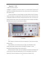
Download TD1262L/C 数字化扫频仪

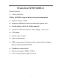
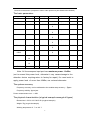
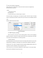
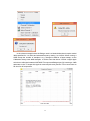
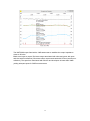
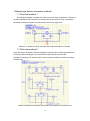
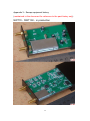
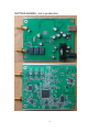
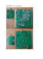
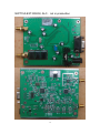
NWT4000-2 RF DIGITAL
SWEEPER & ANALYZER
USER MANUAL
Manufacturer:
WUTONG ELECTRONIC
site：http://bg7tbl.taobao.com
TEL: +86134 2795 9750
Q Q: 1630 2767
Email: [email protected]
version: V2.0
date: 2014-10-20
This document is based on the original manual from the supplier, edited
and updated by Kurt Poulsen (OZ7OU)
The document and applied editing and updates devoted entirely to
document the NWT4000-2 25MHz-4.4GHz unit (using 2xADF4351 PLL’s)but will
also be useful for the NWT4000-2 and NWT4000-1 series going from 138MHz to
4.4GHz (using 2xADF4350 PLL’s). However, the latest NWT4000-2 where the
SMD connector are on top of the PCB (and not at the edge) has improved
screening and far better dynamic range. Watch our when building it into a case
to use a plastic case. Using a metal case will most likely give elevated noise
floor by several dB in the GHz region.
Watch out that you do not purchase the version in a case with two SMA
connectors and a Green LED in between (believing it is a NWT4000 version), as
it most likely will only have 1 PLL (ADF4350 for 138MHz version and ADF4351
for 25MHz version) and thus only is a signal generator and spectrum analyzer,
not being able to sweep the frequency response of devices.
May 2015 edition
1
List of content:
Overview
NWT4000-1 and
NWT4000-2
page 4
Instrumental composition and technical characteristics
page 6
Conditions of use
page 8
The basic design
page 9
1. The hardware connection reference and software guide
page11
1.1 Functions not supported for NWT1400 in the WinNWT software page14
2.1 and 2.2 Logarithmic Y scale sweep frequency settings
page15
2.3 Sweep Calibration
page17
2.4 Blending cursor data into the trace image and saving it
page20
2.5 Typical display of sweep measurements
page23
2.6 Saving of Graphical screen
page24
2.7 unsupported zoom function
page25
2.8 The frequency tag set of cursors
page25
2.9. The Y settings in the Graphical Display
page27
2.10 Bandwidth display settings
page28
2.11 Multi curve display management
page30
3. Linear scan settings (not supported)
page33
4.1 SWR measurements
page33
4.2 SWR Frequency settings
page33
4.3 SWR Calibration
page33
4.4 SWR Measurements examples
page36
4.5 Bridge performance investigation
page37
5.1 SWR_Ant function (not supported)
page39
6.1 Numerical Impedance measurements
page39
6.2 Selection of impedance measurement mode
page39
6.3 Reading from chart the numerical impedance values
page40
7.1 Filter test method 1
page41
7.2 Filter test method 2
page41
7.3 RF transformer measurement method 1
page42
7.4 RF transformer measurement method 2
page43
7.5 An antenna measurement method
page43
7.6 The small capacitance, inductance measuring method
page44
7.7 Amplifier amplitude frequency characteristics measuring
page44
7.8 Notch filter test
page46
9.1 Spectrum Analyzer functionality
page46
2
10.1 Wattmeter Functions
page48
10.2 Wattmeter calibration
page48
10.3 Saving a single or several Wattmeter measurement
page52
11.1 VFO signal level on the output
page54
11.2 VFO frequency setting
page53
12. Frequency calibration
page55
Appendix 1: FAQ
page59
Appendix 2: return loss, reflection coefficient, voltage standing wave
conversion tables.
page66
Appendix 3：Sweep equipment history
page67
Appendix 4 NWT4000 Sweep flatness and frequency calibration
page77
Appendix 4.1 Flatness calibration
Appendix 4.2 Frequency calibration
page77
page81
3
Overview NWT4000-2
Sweep Features
★
35MHz-4400MHz
35MHz - 4400MHz range of fast and accurate measurement
★
Dynamic range: >70dB
★
Software calibration function to reduce the system error
★
Directly display 3dB, 6dB, 60dB bandwidth
★
Curves of maximum minimum value display，with cursor
★
VFO output
★
Power meter function
★
SWR measurement
★
SWR measurement of Antenna with coax feed line simulation
NB not supported by NWT4000
★ Impedance measurement
★
Spectrum Analyzer 35MHz- 4.4GHz
★
Print of measurement data and curve
4
Overview
NWT series digital virtual frequency sweeper is a high intelligent RF
frequency analyzer. The equipment is composed of MCU, RF detection,
RF generator(s), and the circuit board contains the linear detection, log
detection, completely analyzing systems for amplitude versus frequency
characteristics. The amplitude frequency characteristics can be fast and
accurate measurement of RF devices in the 35MHz - 4400MHz range.
NWT series of digital virtual measurement scanner will by way of
man-machine dialogue, display of the numbers on the screen, and can
also print out the measurement data and the curves. The instrument has
the function of self checking, through the host computer and related devi
ces, perform self calibration, so that more accurate measurement can be
done, computing power, and perform signal generator function.
NWT series digital virtual frequency sweeper can be widely used
within radio, television, communication and other fields. The measured
object includes RF Devices like coaxial cables, amplifiers, combiners,
amplifier modules, filters, attenuators, splitters, loads, antennas, powerdividers, and tuners.
NWT series of digital virtual frequency units are sweepers equipped
with microwave integrated circuits and digital integration technology,
controlled by the high performance CPU being a software instrument,
and has the advantages of simple operation, reliable and easy to use
by amateurs, RF developers, television equipment manufacturers, and
being the best choice for RF measurement research institute.
5
Instrumental composition and technical characteristics
Instrument:
NWT Series sweep instrument
1PCS
USB cable
1PCS
AC (100-240V) to DC 12V power supply
1PCS
DISC
1PCS
SWR BRIDGE (OPTION not included)
1PCS
40db ATT (OPTION not included)
1PCS
6db ATT (OPTION not included)
1PCS
The version with improved screening as shown above was
purchase from cart100
http://www.cart100.com/Product/40865867643/
6
7
Technical characteristics (comparison chart to other products by WUTONG ELECTRONIC)
The basic parameters
type
frequency
step
log
line
power
att
ALC
NWT25-EX
2k-25M
1Hz
>70dB
no
12V/0.4A
0-50dB
no
NWT25-USB
2k-25M
1Hz
>70dB
no
USB(5V/0.4A)
0-50dB
no
NWT70-EX
50k-85M
1Hz
>70dB
0-0.7VRM
12V/0.4A
0-50dB
yes
USB(5V/0.4A)
0-50dB
NO
12V/0.4A
0-50dB
yes
USB(5V/0.4A)
0-50dB
NO
12V/0.5A
0-50dB
no
12V/0.5A
0-50dB
yes
S
NWT70-USB
50k-85M
1Hz
>70dB
0-0.7VRM
S
NWT150-EX
50k-300M
1Hz
>70dB
0-0.7VRM
S
NWT150-USB
50k-300M
1Hz
>70dB
0-0.7VRM
S
NWT500-DDS
50k-500M
1Hz
>60dB
0-0.7VRM
S
NWT500-PLL
50k-500M
10Hz
>60dB
+DDS
NWT3000
0-0.7VRM
S
138-3000
1kHz
>50dB
NO
USB(5V/0.4A)
NO
no
1kHz
>65dB
NO
12V/0.5A
NO
NO
1kHz
>65dB
NO
12V/0.5A
NO
NO
M
NWT4000-1
138-4400
M
NWT4000-2
35-4400M
Note: All the sweepers input port has maximum power: 10dBm
(not to exceed this power level, otherwise it may cause damage to the
detection device requiring return to factory for repair). If a need exist to
apply power level of more than 10dBm, use external attenuator.
The system accuracy
Frequency accuracy: can be calibrated to the smallest step accuracy：3ppm
Frequency stability: 3ppm/year
Power measurement error: + -2dB
The physical characteristics (a typical example amongst all types)
Dimensions: L*W*H=113.5*92.5*30 (a typical example)
Weight: 75g (a typical example)
Working temperature: 0 ℃ to +40 ℃
8
Installation and storage
Conditions of use
NWT series digital virtual frequency sweepers are using USB or external DC
12V power supply, and need to be kept away from strong radiations (high power switching
power supply, high power RF emission).
Operation temperature: 0-40 degrees centigrade.
Preheating:
NWT series digital virtual frequency sweepers are most accurate after 30 minutes
preheating prior to measurement.
Storage
Clean up the NWT series digital virtual frequency sweeper container, filled with
desiccant, can be stored at ambient temperature -10 to +50 ℃.
9
The basic design
Hardware configuration
1.1：
Theory:
The block diagram only for reference, some sweepers does not have att. and
amplifier.
The NWT4000-2 contains addition circuitry such as two PLL signal generators but
does not contain any attenuators or Amplifier.
1.2
Hardware connect
With the DC-12V and RS232/USB connected, external devices are connected
to the SMA connectors. (If the power supply method is via USB, as for other type of
products, you only need to connect the USB plug but the NWT4000-2 uses external
DC-12V supply)
NOTE: The supply must we a clean source and voltage can be reduced to 8V to
reduce temperature of the 5V regulators cooling fin, which else being quite hot.
The power connector shall be with positive center.
10
Top view (note new position of SMA Input and Out)
Bottom view (with latest improved screening)
11
The hardware connection reference map
The software guide
Software installation and configuration.
Dependent your operating system, the USB driver might be installed automatic. Let the
computer search on the Internet and it might take several minutes.
Otherwise find on the supplied disk relevant drivers:
If not installed automatic then:
Install USB driver by running ftdi_ft232_drive.exe for WIN7, WIN8 or use
inf file install driver.
Double click install USB driver
1.1 WINNWT
Install WINNWT software
first
，
second
After installing the WINNWT, the attribute shortcuts on the desktop can be modified
to support a number of languages as described below.
Right click on the shortcut and select properties and perform the modification as
described.
However, you may experience problem installing the software supplied on the Disk due
error messages. Copy the two zip files to your hard disk and unzip those, and remove the
Chinese character in the folders/filenames. That worked for me to install the 4.09 version
and the 4.09.07 update. In any case it is recommended to use the latest published version
4.11.09 of WINNWT from below link, as several more and improved features available:
http://www.dl4jal.eu/hfm9.htm. That version used for this documents screendump.
12
Original Chinese startup settings (remark the app cn.qm extension to winnwt4.exe)
The line “G:\Program Files\AFU\WinNWT\winnwt4.exe" app_cn.qm
Changed to:
“G:\ProgramFiles\AFU\WinNWT\winnwt4.exe” app_en.qm available
close and restart the program and the English menu is available.
The use of English version recommended but Chinese cn), Spanish (es), Hungary (hu),
Netherland (nl), Polish (pl) and Russian (ru) language may be chosen. The native German
language requires no extension after winnwt4.exe”
(the “ required before and after the
path as shown)
1.3.
Setting COM port
Insert the USB into the computer.
Because USB driver is already installed, in the device manager you will find the
corresponding COM port and the allocated port number.
13
The port number to remember in this case is COM4.
When installing the driver, on different computers the COM port number will be differ
ent
In WINNWT software "Settings", "Options", select the corresponding COM
port, and click "OK".
Select COM port
Choose the correct com port and if successful, you will see the hardware firmware
version. Otherwise, check the connection and incorrect settings.
Correct prompt after selection of the correct COM port
14
When using NWT3000, NWT4000-1 or NWT4000-2, you must set frequency multiply to 10
rate in Settings/Options.
Note the settings for start and stop frequency where stop is negative. Note also the max sweep
setting. If One Chann. tickmark in Channels is removed then you have two channel operation, e.g.
quite handy to have two different calibrations in actions. Also select Math. Corr. to allow SWR
itteration.
1.1 Functions not supported for NWT1400 in the WinNWT software by DL4JAL
The WinNWT software developed by DL4JAL was for another project and has a number of
function not supported by the NWT4000 family of products. These are:
-
In the Settings Options a number of fields are not supported:
Only Basic_data/Sweep is supported. SA(1), SA(2), General has no functions
Attenuator has no function. Channel. 1 Lin not supported (only Log).
Remark file name for Channel 1 and Channel calibration files can be entered in
the text field so in use when program started. (here CH1-6dB.hfm)
15
-
In the mode selection box under sweepmode only sweepmode, SWR and
Impedance-|Z| is supported. The remaining selection cannot be used as they are.
Attenuation and Frequency Zoom cannot be used.
Display shift OK for the dB Y Axe. Interrupt (uS) = rest time for each sample
-
For the Graph-Manager all functions supported
-
For VFO: Attenuator 0-50dB , Set IF for Sweeping and IF setting has no function.
-
For Wattmeter the VFO on/off does not stop the output but allows to type remarks
and save these. Do not save in the application path but under a folder of your
choice as else hidden for later retrieval.
-
The calculations and Impedanzanpassung (impedance matching) are with no
comment.
2
Logarithmic Y scale sweep frequency settings
2.1
Select the sweep frequency mode
Select the sweep frequency mode
2.2 Set the frequency parameter
Enter the start frequency, the end frequency, scanning numbers / number of
samples for a scan. There are two kinds of scanning modes, a continuous scanning
where the number of samples (max 9999) are being scanned, until final sample to
stop scanning is measured.
16
Another is the single scanning where only one scanning performed for the number
of samples. For changing frequency settings, scanning numbers/number of samples
and other parameters, you must click on Stop before change settings.
The scan delay for each point/sample of the output frequency, are long latency
for power measurement.
Enable the Math. Corr. Channel1 (and Channel2 if enabled)
Y scale and Shift can only be set, provided the scan is stopped.
Attenuation is not applicable for the NWT4000 models
Other possible settings to be explained in later sections of this document
17
2.3 Before starting measurement the Instrument should be calibrated.
It is recommend to initially using the software on the supplied disc called COM assiter.exe.
It performers an excellent flat calibration of you particular hardware and the result is saved
into the hardware. However the levels from -10dB to 0dB is nonlinear due to about 4dB
compression in the internal reception mixer and/or logarithmic detector. The -40dB level is
calibrated and consequently the -10, -20 and 30dB level are not fully accurate. It applies
also for all levels below -40dB. This problem can be eliminated by inserting a 6dB
attenuator in the Output path (mounted on the SMA TX output at all times) but this
however reduces the dynamic range by 6dB. As the WinNWT software also have
calibration routines, which is allowing the top level calibration, to be performed at a user
selected lower level this 6dB attenuator is only used during calibration within the WinNWT
software and removed after calibration. Then the full dynamic range is available with the
only limitation that 0dB level is compressed to about -3dB but from -10dB and downwards
everything is perfect. If the device tested has an insertion loss above 3-4dB then the
compression has no effect. If not so then use a 6dB att. permanently and accept the 6dB
loss of dynamic range and create a different calibration.
The WinNWT software can save as many calibration files as you wish so just find you own
way.
The initial calibration being the platform the WinNWT calibrations is described in the
document “Calibration step_UK.pdf” published same public places as this document. The
documentation also added as Appendix to this document. It also contains a frequency
calibration method, which works nicely and allows 1KHz setting at 4.4GHz (but that
stability not maintained over time or temperature changes).
The frequency calibration is performed at 1GHz and the measured output frequency just
entered in the WinNWT DDS (PLL) clock field, as seen previously above on page 12 as
999999800Hz. Tricks a possible to use a 100MHz counter as described in said document
and the Appendix.
A WinNWT calibration performed as follows
Select Channel 1 Calibration and subsequently Logarithmic Channel (Lin does not apply
for NWT4000 hardware):
18
Insert a 40dB attenuator in the Transmit path (at the SMA Output) and click OK
Subsequent you are promptedd to insert a 0dB attenuator or select differently a user
defined att. here stepped down to -6dB. The sweep is performed automatic with 9999
samples.
Then you are asked to save the calibration or not.
(if not then only in force as long the NWT4000 switched on)
A file name selected here CH1-6dB.hfm
19
When accepted by a click on OK the trace is jumping to it correct position -6dB. If Y
scaling change to 0 and -10dB we see it bang on -6dB (small image below)
If we enter the 40dB att. and run a single scan, we will see it is flat on -40dB from 35MHz
to 4.4GHz
If we connect the Output and Input directly and run a sweep we see the degree af
compression in the mixer. Below 2GHz it is about max. 2.5dB and above 2GHz it is
reduced to less than 1 dB. By clicking on Graph Manager we can maintain the sweep by
clikcing on Get and enable tickmark Active Channel 1 and Active as shown. Thus we can
have up to 6 traces for ch1 on the screen in addtion to the current run sweep.
As can be seen below the linearity is quite excellent and the noise floor pretty low
20
2.4 Blending cursor data into the trace image and saving it
It is possible to blend cursor data into the trace image. First of all press the numeric
key from 1 to 5 on the keybord and click on the frequency position where you want the
particulator cursor number to be placed. When so done select in the main menu File /
Speichern als Bild (store as image). When next screen promt apears enable tickmark
“Info einblenden” and with X and Y position, place the information where you want it.
You may also change letter size with Schriftgroesse. When you click on the “Bild
speichern” you can save the image to harddisk incl. the data information as shown
below.
21
You may edit first line ;no_label prior to “einblenden” as seen on the next image below.
22
Above measurement done with two 5cm long male SMA SMA cables connected from
the PCB SMA connector to a front panel with female female SMA adaptors used as
the TX and RX connections. As previous described the NWT4000-2 has best
dynamic range if mounted in a plastic case. Below plot shows a calibration performed
without these two 5cm MSA SMA cables and the female female adaptors, thus directly
at the PCB SMA adaptors and the dynamic range even better manintaning 80dB to
4.4 GHz.
To utilized the NMT4000-2 to the extreme two male female SMA adaptor might be a
possiblity to get the Input and Output to penetrate the case on the top and let the
cooling fin be exposed to the ambient.
The black trace for Input and Output directly connected shows below 3GHz up to 2dB
loss off signal amplitude due to mentined compression in the internal mixer and/or
logarithmic detector. If the DUT has insertion loss more than 2 dB it has no effect.
23
2.5 Typical display of sweep measurements
WiFi Filter single Channel
24
A single scan curve, the curve is a curve of a 21.6M filter
2.6 Saving of Graphical screen
The Grapical Screen can be saved and re-loaded by clicking on Graph.
The format is *.hfd and saving can happen to a folder at your choice.
25
2.7
The below mentioned function about frequency zoom is not
supported by the NWT4000 series and only mentioned for reference.
2 times zoom settings
For a measurement, the available frequency scaling functions are magnified 2 times,
reduced 2 times, fast frequency response measurement device. The + button 2 times
magnification operation, bond was reduced 2 times operation.
2.8 The frequency tag set of cursors
Select with Curcor #, in the drop down list, either 1,2,3,4 or 5, and on the
Graphical Display, with a click of the left mouse button, where the marker is
desired to be positioned. On the Graphics Display area will be displayed an inverted
triangle, and in the text area, the marker frequency and corresponding amplitude will
be shown. By a right click on the Graphical display you may delete a single or all
markers. The Cursor # can also be selected by tapping the corresponding number
on the PC keyboard, as a shortcut to the frequency tag setting.
Select the 1-5 Icon in the drop down list
26
Inverted triangle marker displayed
Frequency of the 5 screen markers displayed, and the signal level in dBm
27
2.9. The Y settings in the Graphical Display
The Y axis scaling function:
The Ymax signal level on the Graphical display is selected in the drop down list.
Standard level is 20dB but 0dB more relevant for the NWT4000 family
Ymin signal level on the Graphical display is also selected in a drop down
list, generally choose -90dB. Fine adjustment in 1dB step is also selectable.
Y axis scaling function
To magnify the top area of a trace you may change the settings to Ymax=0dB
and Ymin= -20dB. Note that, because of the limited resolution of the MCU AD conver
sion the curve may appear “stepped” / jagged as seen below.
Select back to Ymax=0dB and Ymin=-90dB
28
Measurement of a 49.55MHz Quartz Crystal
2.10 Bandwidth display settings
The measured curve, can directly have in the Graphical Display the 3dB, 6 and 60dB
bandwidth shown as lines and the data shown in the text field with additional Q value and
rectangular coefficient. Tick mark the required function in the Bandwidth selection box. A
tick in “Markerlines” toggles all the marker line presentations in the Graphical display on
and off.
Bandwidth selection
6dB/60dB and 3dB/Q tick, the software will display the measured curves
3dB bandwidth and Q value. On above image the Q value calculated for a 49.55MHz
quartz crystal and below for the WiFi filter remark the 60dB on the high side of the curve is
way off because the notch is not 60dB deep enough some 56dB relative top level at
marker 1.
29
The measured curve
Display of 3dB bandwidth, Q value and related
parameters
6dB bandwidth and 60dB bandwidth, is similarly
rectangular coefficient.
Markerlines are used to display the dotted line
bandwidth in the Graphical Display area, for better
recognition of bandwidth parameters.
B3dB Inverse is used for trap measurement.
30
2.11 Multi curve display management
Graphic-Manager Get；Active channel；Show Graph
After a measurement, the curve can be stored and controlled by the Graphical
Manager. The current trace is acquired by a click on the Get button. Then tick the active
channel number and tick Active for Showing Graph.
Version 4.11.09
Graph-Manager
31
Version 4.09.07
Version 4.11.09
Graph-Manager
32
Version 4.09.07
3 traces selected for presentation for a 500MHz diplexer.
Low/High pass and Isolation (red)
The Graphical Manager is quite handy for measuring e.g. diplexers. As the first graph for
this diplexer (specifiied as 0-500MHz/800-1300MHz) showed many spurious responces in
the 35 to 500MHz region. As the NWT4000 deliver squarewave signals as the output
signal, the 3. and 5. harmonics (or even higher orders) passes unattended throught the
higpass filter. By inserting a 500MHz (black trace) or 600MHz (red trace) low pass filter,
only the 3. harmonics of 250MHz is visible and the true resonce of the the diplexer below
600MHz found.
33
3. Linear scan settings (unsupported)
Note: Some type of equipment do not have this function and are not supported by
NWT4000 family of products.
4. SWR
4.1 SWR Measurements
Enter SWR mode
For SWR measurement an external brídge is required.
Connect the bridge. The bridge input is connected to the NWT scanner RF output, The bridge
output is connected with the NWT scanner RF input. See later for the calibration method
used.
Select the SWR measurement Mode
Test mode select
4.2 SWR Frequency settings
Set the frequency and log the same scanning pattern. Enter the start endpoints,
frequency, frequency, continuous or single measurement can be read directly of the SWR.
The need for accurate calibration for measuring needed.
4.3 SWR Calibration
With bridge properly connected and the output of the bridge either shorted or open select
Sweep/Channel1 Calibration. With bridge none terminated the calibration is started by
clicking on OK. The number of samples automatic changed to 9999 and after a while, you
are asked to save the calibration under a descriptive name.
Then at any time you can recall the calibration by “select Channel 1” in the menu shown,
and choose the calibration file previously saved.
34
In the shown example below the Bridge used is a Narda bidirectional coupler model
3022 specified for 1 to 4GHz and selected frequency setting 1 to 4.4GHz. When running a
SWR sweep the number of samples is e.g. changed to 999 for a faster sweep, as the
Calibration always uses 9999 samples. It will be seen that above 2.5GHz a slight ripple
exist due to reflection between NWT4000 TX output and Bridge input. By inserting a 10dB
attenuator in the TX output this ripple is removed (red trace) and the TX out now closer to
50 ohm for all frequencies.
35
Black trace without any attenuator in the TX path and red trace with 10dB attenuator
inserted. The bridge output is -20dB below input signal and as there is ample sensitivity in
the RX so this 10dB attenuator does not harm. Please observe the SWR range can be
changed with the drop down list.
DUT
36
4.4 SWR Measurements examples
The GSM900 band between marker 1 and 2 has too low a resonance and then too
high SWR but GSM1800 inside marker 3 and 4 quite OK
The picture below is a measurement of a UHF low band antenna. The resonant point
at about 430M, SWR about 1.1. The related limit values are to read in the text area.
The measured antenna curve
37
The text area shows the standing wave maximum, minimum
Another case of a 3.5GHz 10dBi vertical antenna with and without 4m feed line cable
4.5 Bridge performance investigation
Is is also posssible to examine the Bridge for proper operation to be used for SWR
measurements.
Run a sweep for the bridge from input to output and also for the bridge coupler
output with the Bridge output terminated with open, short and 50 ohm.
38
The NWT4000 output fitted with a 10dB attennuator to stabilize the output impedance
closer to 50 ohm.
Black trace input to output. Red trace output terminated with short and green with open
and thus with full reflection). Blue trace when output terminated with 50 ohm (and thus no
reflection). The span from terminated with 50 ohm and short/open is better than 30dB
yelding adequate span for SWR measurements.
39
5 SWR_Ant mode
5.1 SWR antenna measurement with coax feed line
This function is not compatible with the NWT4000 family.
Setting the cable parameters
Wrong results obtained if used
6. Impedance - |Z|
6.1 Numerical Impedance measurements
You need to use the bridge to measure the numerical impedance. During the
measurements you need to insert a 50 ohm resistor in series with the DUT. This means if
the bridge is terminated with 50 ohm the reading is 0 ohm.
Do not measure impedances directly as impedances below 50 ohm also will give
positive readings.
SWR calibration required if not already performed prior to measurement of the DUT.
For the SWR calibration procedure see section 4.3
6.2 Selection of impedance measurement mode
After calibration, select the impedance measurement mode
Selection of impedance measurement model
After selection read the prompt and then ignore.
40
6.3 After measurement read directly from the chart the numerical
impedance values
During measurement a 50 ohm resistor in series with bridge and
DUT required.
Measurement of a 65 ohm resistance.
41
7 Measuring a device connection methods
7.1 Filter test method 1
The following diagram is suitable if the filter input and output impedance is 50 ohm, if
the filter impedance has mismatch, the measurements are prone to error in passband
bandwidth and big fluctuation of measurement inaccuracy might exist.
.
Methods 1, suitable for filters with input and output impedance of 50 ohm.
7.2 Filter test method 2
If the filter does not need the 50 ohm impedance matching then matching transformers
introduced. After matching the curve and filter measurements was accurate.
Resistance matching can also be used, but the matching method introduces very large
insertion loss.
Method of impedance matching, this method can measure the insertion loss
42
7.3 RF transformer measurement method 1
RF transformer measurement method 1
7.4 RF transformer measurement method 2
RF transformer measurement method 2
43
7.5 An antenna measurement method
For NWT series of frequency sweep meter you need an additional external bridge for
antenna SWR measurements. A reference circuit are as follows:
ANTENNA
RF OUT NWT4000
RF IN NWT4000
diagram of SWR bridge
Because the bridge needs to be a precision device, not easy to make yourself, you
are recommended to buy a finished bridge. The finished bridge pictures are as follows:
Swr bridge
In below diagram is shown a frequency sweep with logarithmic Y scale (in sweep
mode) measuring an antenna, connected to the bridge output, and a dip seen where the
antenna has resonance just like when measuring in the SWR mode.
VHF antenna measurement curve with a bridge
44
7.6 The small capacitance, inductance measuring method
Testing of unknown L or C
7.7 Amplifier amplitude frequency characteristics measuring method
If it is a small power amplifier, and the output power is less than 10dBm, you can
directly connect to the sweeper’s RF OUT and IN without to destroy NMW4000 series.
However as seen before the INPUT saturates for a lesser amplitude so attenuator needed.
If the power amplifier, needs to be used with the directional coupler or attenuator for signal
attenuation, then enter the attenuators in the detection circuit (RF IN).
During measurements you need to pay attention to the amplifier and load impedance
matching. For the power amplifiers, you need to pay attention to frequency scan range
which should not be too broad, otherwise the amplifier impedance changes, standing
wave increase, and easy to cause damage.
Amplifier test method
45
Power amplifier test 1
Power amplifier test 2
46
7.8 Notch filter test
For a trap LC parallel circuit, available method for testing shown where a dip seen in
the sweep mode when connected between RF OUT and RF IN.
LC parallel notch filter measurement connection method
9 Spectrum Analyzer
9.1 Spectrum Analyzer functionality
The Spectrum Analyzer is a simple spectrum analyzer which is utilizing one of the PLL’s in
the NWT4000-2. Quite simply the spectrum analyzer is no less than the sweeper where
the signals to be analyzed is applied to the Input Port. The PLL delivering signal for the
receiver mixer (receiver PLL), is running with a fixed offset from the wanted frequency of
260KHz, to facilitate the sweeper is measuring on the right frequency. The PLL being input
to the RX mixer, beats with the RX input signal and generates an IF signal on either side of
the input frequency, but not being on the required frequency. The IF signal is passing
through a low pass filter from 15KHz to 300KHz and being detected in the Logarithmic
detector for presentation. The other PLL on the TX side is doing nothing when we are
analyzing the spectrum. Below is shown an input signal of 100MHz from the Marconi
2022A Wavegenerator stepped down in 10dB steps which discloses the Offset between
the two PLL’s.
47
Spectrum of the 100MHz signal when -6dBm, -16dBm and -26dBm applied to the input
It is clarly seen that all sort of spurous signal generated and mesurement of the signal
generators harmonics not possible. First by comparing the -16 and -26dBm sweeeps we
can trust the measurements of 2. - 3. - 4. and 5. Harmonics.
48
10 Wattmeter
10.1 Wattmeter Functions
The Wattmeter, when calibrated, is a superb tool as being a selective
Wattmeter only measuring the frequency the VFO is tuned to, with a bandwidth
of 300KHz to either side of the VFO frequency and then suppressing
harmonics and other signal which could create false readings. Tools are
provided to compensate for the slight drop off sensitivity above 2.5GHz.
Before selection the Wattmeter remember to select the calibration file for
“sweep” as calibration data for Wattmeter is stored in the sweep calibration file.
Please also do the sweep calibration first before the Wattmeter calibration.
In this case the Select Channel 1 filename is CH1-6dB.hfm chosen, where the file
name indicates the sweep calibration performed using a 6dB and a 40dB attenuator
as the NWTWin software facilitates to obtained a superb dB linearity.
You might have saved the sweep calibration in the default file name defsonde1.hfm
10.2 Wattmeter calibration
Note: For NWT4000-1 and NWT4000-2 the VFO must be set to the frequency to
measure.
Now select Wattmeter and apply a signal source, with known dBm amplitude, to the
NWT4000 Input port. You may also chose the signal source to be the NWT4000
output but insert preferably a 20dB attenuator in the signal path, however at least 6dB,
to avoid the compression in the mixer/logarithmic detector, of the internal circuitry, as
described earlier page 16 under sweep calibration . Observe the dBm reading is pretty
49
wrong as the Wattmeter not yet calibrated. Below the dBm read out is a drop down list
which indicated is is possible to compensate for variation in the sensitivity of internal
detection circuitry across the 35MHz to 4.4GHz range, but as seen the list is initially
for a quite different product, so the calibration needed both to edit the drop down list
and the sensitivity and the procedure described below
When for Wattmeter we click on ”Measurement” the drop down list allow a number of
selections. DO NOT CHOOSE “Channel 1 Calibration” as NWT4000 does not
support this procedure of the WinNWT software. We will instead choose the “Edit
Channel 1 calibration” as perform the calibration manually and edit the prompting as
well in the compensation drop down list in a couple of steps.
When chosing the Edit Channel 1 calibration the initial setting is seen below next to
result the final settings to be explained in the next steps.
50
The input to the NWT4000-2 when delivered from the NWT4000-2 output is measured
to be - 2.36dBm with a Hewlett Packard powermeter 437B and 8481A power sensor.
As the output of the NWT4000-2 is squarewave the theoretical fundamental is 0.707
or 3.01dB lower in level then -5.37dBm. As we have 20dB inserted in the signal path
and measures – 7.7dBm with the Wattmeter then the theoretical compensation to
apply is 20 – 7.7dB = 12.3dB. The picture above to the right shows a compensation of
15.20dB which is derive when using the signal from a Marconi 2022A Wavegenerator
with an accurate measured sinusoidal output of 0dBm using the HP437/8481. I seem
like the NWT4000-2 output is not following the theoretical condition and the third and
higher harmonics are lower than theoretical levels explaining the difference. It appear
the difference is only 1dB. As the output impedance from the NWT4000, deviating
somewhat from 50 ohm it is contributing to some mismatch as well.
Anyway when using the Marconi 2022A wave generator up to 1GHz with accurate
measured output, and the output from the NWT4000-2 from 1GHz to 4.4GHz where
output measured with the HP437A as well, the compensation derived as shown in the
below image, across the frequency band. The NWT4000-2 VFO is covering 2.2GHz to
4.4GHz and sub-band created by division of 2,4,8,14,32. These limits entered in the
edited list. However above 2.2GHz further sub band created according to the
measured levels drop off, as seen in a Graph further down. All the data from the
editing is automatic saved in the current selected sweep calibration file, when clicking
on Save in below screen.
51
The editing thus results in a new visual drop down list
If you do not have a wave generator then use the settings in the table. It is better than
nothing done.
52
Interesting to see the peak at 1.1GHz which is reflections inside the PCB of the
NWT4000-2 as well a 5 cm SMA male male cable can create 1.5dB attenuation at
2.8GHz. Also observe that when using an external 20cm SMA male male cable that
standing waves develops above 1GHz and how a 10dB attenuator is stabilizing the
frequency response with the 20cm cable present.
10.3 Saving a single or several Wattmeter measurement.
In case you want to measure a number of Wattmeter levels e.g. at 100MHz the output
of an oscillator for various supply voltages or, as in this example, the levels for a step
attenuator at various attenuations and later import these data into a spreadsheet, you
can add each measurement to a table and when finished save the table to a file.
53
As there is inserted an 10dB attenuator in series it can be compensated for by the
“Attenuation (dB)” setting.
Select for each measurement “Write to Table”
When finish with the measurements select Save Data and chose the location for saving
and provide a file name.
The format of the data in the saved file is semicolon seperated and directly to import in
e.g. Excell.
As neither the frequency nor step number is included in the data (left picture) such
information must be added manually (right image)
54
11. The VFO mode
11.1 VFO signal level on the output
The output is documented in section 10.2 page 52 as the level into 50 ohm
11.2 VFO frequency setting
The frequency setting is quite simple to understand and need no further explanation.
They is selextion possiblity for five quick access frequencies which in combination with
the tick in VFO-Frequnecy x4 for “I/Q Mixer” (as VFO for a SDR radio), where the output
frequency is 4 times higher then the setting, can be quite handy for quick band changes
The minimum frequency steps are dependant of the frequency and the dicvision rate in
the PLL going from 1:1 , 1:2 1:8 1:16 1:32 to 1:64 for the lowest band
From 2.2GHz to 4.4GHz they are 1KHz
From 1.1GHz to 2.2GHz they are 500Hz
from 550MHz to 1100MHz thety are 250Hz
From 275MHz to 550MHz they are 125Hz
From 137,5MHz to 275MHz they are 62.5Hz
From 68.75MHx to 137,5-mhz they are 31.25Hz
From 34.375MHz to 68.75MHz they are 15,635Hz
That os not entirely the thruth because the PLL is binary and not exactly in 1KHz steps.
55
12. Frequency calibration (Note!! Read appendix 4 if you counter only
can measure 100MHz)
12.1
Prepare a 1GHz frequency counter, allow enough warm-up time, for NWT4000
electric power up for 30 minutes（NWT3000，NWT4000-1.NWT4000-2 used 1GHz
calibration, for others models use 10MHz calibration）
12.2
Enter VFO mode , output 1GHz/10MHz
Input 1GHz/10MHz
3
Use frequency counter to test nwt4000 output frequency
Test output frequency in this case 999.990 330MHz
56
4
Enter option
Enter OPTION
5
Input frequency counter frequency with units in Hz, press OK, then the frequency
calibration is complete, result as shown below.
57
Input test frequency
Frequency reading has changed
Frequency calibration complete.
58
The user should pay attention to:
1. Read the manual at first.
2. NWT series digital virtual frequency sweeper is a precision instrument and
has been vibration tested, splash proof, and corrosion resistant.
3. Do not short circuit signal the output port, as easy to cause internal damage
to parts.
4 During testing, do not use a soldering iron in the device under test.
59
Appendix 1: FAQ
1. What is this device used for ?
A sweeper is a frequency characteristic tester, it is a test set which test devices for
frequency and amplitude characteristics as curves, such as test of a LC tank’s frequency
and amplitude curve.
2. What is the difference of a NWT sweeper and a BT3 (CHINA TYPE) CRT sweeper.
A NWT serial sweeper is a digital sweeper, with small frequency steps, connected to a PC
via USB which performs the calculation of data and present the curves. It can act as VFO
(signal generator) and as a power meter and are lighter than the old sweeper. NWT4000-1,
NWT4000-2 can be used as a simple spectrum analyzer.
CRT sweep
3,
NWT sweeper is connected to the PC but non-responsive，How to know the sweep
analyzer is OK?
Check USB driver, check external DC power supply, check USB cable, check
software setting about what port number is allocated to the sweeper in control
panel/system/hardware settings. When responsive then:
Disconnect input and output. The curve is displayed in the bottom of the display area.
Connect input and output with shielding cable. The curve is displayed in the top of the
display area. If these two displays/curves are normal then the sweeper is OK.
60
4, Can the sweeper test a duplexer and how to test ?
A duplexer is a filter. The NWT sweep analyzer input is connected to the output
of the duplexer antenna connector and the NWT OUT connected to the Low or High
antenna connector (the unused connector terminated with 50 ohm). The high and l
ow frequency response thus measured as shown below.
Duplexer for UHF band
GSM band duplexer
61
GSM band duplexer curve
5，How to test antenna ?
Used a SWR bridge or a three port connector.
SWR bridge test:
Swr bridge, RF output
62
Diagram
When using the SWR bridge you can measure in the transmission sweep mode, as a
qualitative measurement, but you need to pay attention, frequency sweep analyzer can
only use the RF Output of the Bridge, not the Bridge band detection output.
63
SWR bridge test of UHF antenna with three port connector
Use a three port connector replacing the SWR bridge, and you can test an antenna ,
but only for a qualitative test just a showed above
SMA three port
6. Attention when using the Sweep analyzer.
.
When connected to the computer and the DUT, then you need to pay attention
that grounding is good, to prevent too high level input to the detection circuitry, otherwise
it will damage the detecting element.
7. Power supply from the USB port is inadequate, what to do?
According to USB2.0 protocol the current is 0.5A, which should be enough. If the USB
power is not enough, check USB cable connection is good, or change to a high quality
USB cable, change to a USB 3.0 port (current is 0.9A) or use an externally powered USB
HUB.
8. The impedance is not matched, creating problems, how to solve.
If there is an impedance mismatch, power is not 100% transmitted, and reflection
will cause the measured parameters (gain, fluctuation, insertion loss, bandwidth) and
other parameters being incorrect, then you can consider using external transformers or
resistors as impedance matching, then measure again.
9. I need to improve the NWT input and output impedance precision, how to do ?
Insert an inline attenuator in the instruments input and output terminals, attenuator
64
normally of 3 dB will be adequate but if you want to have more precise, they can be
replaced by 6-10 dB attenuators or even higher dB levels but the disadvantage is loss of
dynamic range.
10. Some component curves tested with the NWT4000-2 equipment
HP 5086-7051 LPF
Mini NHP-700 HPF
65
REACTEL 1.1-1.15G BPF
BPF24-806A
66
Appendix 2: return loss, reflection coefficient, voltage
standing wave conversion tables
67
Appendix 3：Sweep equipment history
(maintained in this document for reference to the past history only)
NWT70，NWT150，in production
68
NWT500-DDS AD9957, in production
69
NWT4000-1，NWT4000-2, in production
70
NWT500-AD9958-, not in production
71
NWT500-AD9858-, not in production
72
NWT500-PLL+DDS, not in production
73
NWT3000，not in production
74
NWT70-USB, ALC，not in production
75
NWT150-EXT-RS232, ALC，not in production
76
NWT70-RS232-EXT, not in production
77
Appendix 4 NWT4000 Sweep flatness and frequency calibration
1. NWT4000 sweep calibration steps
Appendix 4.1 Flatness calibration
ATTENTION: If curves is not flat or the linearity from -10dB to 0 dB is too compressed,
then insert two 3dB attenuation to input and output both when instrument is used and when
calibrated as described below. Then the linearity from 0dB down to -70dB is very accurate.
The dynamic range is of course reduced by 6dB. Alternatively a single 6dB attenuator can be
used and if so then place on the output not to reduce the sensitivity when used as spectrum
analyzer.
1. Connect power and connect USB to PC, Power on for 30 minutes.
2. Opened COM assiter and select COM port
(You may remove the Chinese characters by renaming/editing the file name)
3. Select COM port, baudrate, hex, ASCII code
78
4.
Open COM port, input 8F 60
5. Click on Send
79
6. According to the prompt, “short circuit” input output by connection a SMA male-male test
cable between input and output, and when completed click on Send
7. Insert 40dB attenuation and when done click on Send
8. Calibration complete.
80
9. Calibration complete the curve is flat for 0 and 40dB
81
Appendix 4.2 Frequency calibration
1. Prepare a 1GHz frequency counter, warm-up time enough, NWT4000 electric power up
for 30 minutes
2. Enter VFO mode ,output 1GHz
3. Used frequency counter test nwt4000 output frequency
82
4. Options:
5. Input frequency counter frequency with unit Hz，press OK, frequency calibration
complete。
83
Special tricks if your counter does not go to 1GHz:
If you counter does cover 100MHz then use a gate time of 10sec to read the frequency with at
least 10Hz resolution , set the VFO to 100MHz and write down the measured frequency e.g.
99.99931MHz . Then write down the frequency as if it was 10x higher with 1 Hz resolution
84
e.g. 999999310Hz and set the VFO to 1GHz and enter 999999310 into the DDS (PLL)
Clock (Hz) in the Settings/Options/ menu point. Then the frequency is calibrated to within
1kHz at 4.4GHz. When measuring the 100MHz output after calibration You may experiment
with the 1 Hz settings to get closer to 100MHz. Most likely, you will hit the correct frequency
with less than 50Hz error.
85