1
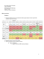
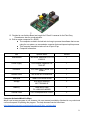
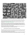
Multicamera Array Documentation Freshman Imaging Project 20122013 Amy Becker, Elizabeth Bondi, Matthew Casella, Ambar de Santiago, William Frey, Alexander Jermyn, Colin McGlynn, Victoria McGowen, Jason Mitchell, Briana Neuberger, Michaela Piel, Elizabeth Pieri, Wesley Robinson, Kevin Sacca, Victoria Scholl, Lindsey Schwartz, Tyler Shelley, Dan Simon, Benjamin Zenker 1 Table of Contents Objective:......................................................................................3 Introduction: …............................................................................ 3 User Requirements: …...............................................................3 Methods of Communication:......................................................4 Outside Communication:............................................................4 Equipment Surveys.....................................................................4 Basic procedures:.......................................................................5 Computer Animated Model In Maya:.......................................10 Software:......................................................................................12 Camera Calibration....................................................................12 End Result:..................................................................................16 Setbacks/Advice.........................................................................17 Important Websites/More Information:.....................................20 2 Multicamera Array with Synthetic Aperture Effect Documentation Objective: The purpose of this imaging science project was to learn about advanced components of an imaging system and basic concepts in designing and building a structure. During the year the class covered topics such as camera characterization, video processing, coding, etc. Introduction: Our assignment for this class was to create a synthetic aperture system using a Multicamera Array to implement at the Greater Rochester International Airport in Monroe County. We wanted to use this system in order to use the different angles of the cameras in order to see around occlusions. At the Airport, we wanted to use our system in the baggage claim area in order see someone taking someone else’s luggage, even if they are hidden behind a column or another person. User Requirements: Airport Requirements: Zoom Not Needed Color Important, but not necessary Field of View Minimum 35 degrees Pan and Tilt Not Needed Frame Rate 15 fps File Size and Processing Speed To be determined ImagineRIT Requirements: Video Type Black and White Movement of Cameras Stationary Movement of Lens No Zoom Number of Cameras 24 Possible Types of Cameras Point Grey: Grasshoppers and Chameleons Webcams GoPRO Pinhole Camera Kodak Cameras Scale Dimensions Small (5x5 feet) 3 Field of View Future Scope Speed Frame Rate 10 fps Data Processing < 1 second Resolution 640p Data Connector Firewire Methods of Communication Methods of Internal Communication Our primary mode of communication was through group facebook posts, because it is frequently visited and easy to use. We also included a second site to communicate information on an RIT wiki page. This was useful for posting papers and documents, but eventually faded out of use in favor of Google docs. Finally, we created a forum in the first quarter that went mostly unused for the entire year. We also had one group in the fall quarter, called the organization group, that worked to try to make the communication between the different groups better, since that is one of the most important parts of a team in order to be successful. Another form of communication was meetings. We would have a meeting with the whole entire class at the end of class on Thursday, to make sure everyone knew what was getting done. Also throughout most of winter quarter, each group would meet with the professors of the class, so we could make sure we were on the right track. Outside Communication: We tried to reach out to the graduate students at Stanford that built the model we were attempting to replicate. We also tried to contact Lytro to assist with the project but they informed us that they don’t partner with colleges due to the large quantity of requests that they receive. We kept in continuous contact with Point Grey support to help us use the cameras and get our systems working. We contacted Dr. Tadd Truscott from the Splash Lab at Brigham Young University and they gave us some of their code that they made for synthetic apertures and a step by step explanation of what their code means and what it does. We kept in contact with security personnel, Brian Wenzel, at the Greater Rochester International Airport in order to figure out what the Airports requirements were for the system and to figure out the location of where they wanted our system to go in the Airport. Equipment Surveys (see more information for links to ppt): Point Grey Camera: Math Theory Foundation: Lytro Camera: 4 Key Imaging Optics Concepts: Video Processing: 8020 Materials and Machining: ImageJ Tutorial: Geometric Camera Calibration: Basic procedures: Hardware: 1. Researched different types of cameras and made a pugh analysis in order to pick which wouldwork best with our array: 2. Researched ways to mount the cameras 3. Tested 4 webcams that were already in the lab ■ Types of Webcams: ● Logitech Carl Zeiss 2MP Autofocus Webcam 5 ● LifeCam HD5001 Webcam ● Philips Webcam SPC1330NC Pro ● Logitech Webcam C200 ■ Reasons we rejected them: they had insufficient quality and had no software to read them from 4. Tested 4 Point Grey Chameleon cameras that we had in the lab ■ Reason we rejected them: They had no compression 6 5. Examined mounting material called 80/20 that we had in the lab ■ Determined it would work well to use to mount the cameras of the system 6. Bought 2 Point Grey Blackfly cameras at $395 each ■ Reasons we bought them: GigE interface, which has a higher bandwidth, and GPIO for synchronization ■ Reason we rejected them: They had no onboard compression, so there was too much data for the computer to process 7. Bought 12 ECam51 cameras at $89 each ■ Reasons we bought them: Onboard compression and GPIO for synchronization ■ Reason we rejected them: They did not have consistent frame rates 7 8. Bought an Arduino Board at $29.99 ■ Reasons we bought it: To help synchronize the ECam51 cameras ■ Reason we rejected it: Some triggers didn’t work with the ECam software 9. Bought more 80/20 for ECam51 cameras ■ After deciding we were going to use the ECam51 cameras, we designed a structure for the system and determined that we would need to buy more 80/20 in order to build the structure we had designed. 10. Bought 2 Point Grey Chameleon cameras at $375 each ■ Tested the 4 Point Grey Chameleon cameras and determined that they maintain consistent frame rates, but wanted 6 cameras in our system, so we ordered 2 more 11. Bought 6 Fujinon DF6HA1B lenses at $134.95 each ■ The Point Grey Chameleon camera does not have a fixed lens and it did not come with a lens, so we had to buy lenses for each cameras. These lenses have a 6 mm lens, which our predictive modeling showed was the best choice. ■ Other lens options we looked at: https://docs.google.com/a/g.rit.edu/document/d/19yWyEGGN7fTQo5V5hSS91bhu BKbfJkqN5j1KaJtA1A/edit 12. Bought 6 Raspberry Pis at $35 each ■ We had rejected the Point Grey Chameleon camera earlier, because they had no compression, so in order to fix this problem we bought a Raspberry Pi for each camera. The point of the Raspberry Pis is to compress the data collected from the camera in order to reduce the data flow into the computer. 8 13. Decided to use Arduino Board we bought for ECam51 cameras for the Point Grey Chameleons, also for synchronization. 14. Built a custom computer for ~$2200 ■ The computer we had in the lab took too long to process the software that we are using for our system, so we needed a computer that would speed up this process. ■ This computer was able to take us from 4 fps to 5 fps ■ Computer Information: Part Specific Name Amount Motherboard MB ASUS Sabertooth X79 X79 LGA2011 1 Power Supply PSU Rosewill Capstone750 750W RT 1 Processor CPU Intel Core I7 3930K 3.2G 12MB R 1 Network Card NIC SYBA SYPEX24028 R 1 Heat Sink Water Cool Corsair H100I 1 Storage SSD 500G Samsung MZ7TD500KW R 2 Memory MEM 4Gx2 Gskill F314900CL9D8GBSR 4 Thermal Paste CPU Thermpaste AS53.5G% 2 Computer Animated Model In Maya Maya is not an easy program to use; however, the user manual provided by Autodesk is very robust and covers all aspects of operating the program. The help document can be found here: http://download.autodesk.com/global/docs/maya2014/en_us/index.html 9 Maya is located on the windows partition of Festiva. Start Maya from either the desktop icon or from the windows start menu. When it opens you should get a splash screen. After the splash screen loads the actual program will load and bring up two child windows, one is a new features highlight settings. You can close that. I highly recommend checking out the startup learning movies especially navigation essentials, moving rotating and scaling objects, and reshape and edit objects. ANYWAYS Start by opening the scene file this is done from the top drop down menus with: File>Open Scene... The most recent version of the scene is located at: C:\Users\FreshmanImagingProje\Documents\maya\projects\default\scenes\Airport Baggage Combined 2.mb Once the file is opened the large version of the airport scene will open. The box that you are viewing the scene through is called the viewport. Navigate to the set of menus on top of the viewport. Select: Panels>Saved Layouts>Persp/Outliner To change the camera you are viewing through, go to the viewport menus and navigate to: Panels>Perspective>”Camera Name” To create a new camera, go to the main drop down menu at the top and select: Create>Cameras>Camera☐ The new camera starts selected, to move it select the move tool from the sidebar or use the ‘W’ hotkey. The other way to move an object a precise distance, go up to the top bar where you see three text boxes labeled ‘X’, ‘Y’, and ‘Z’ respectively. The units for these boxes are scene units (the units the scene was created in. In new files Maya defaults to centimeters however in the airport model, inches were used (sorry!) To rotate an object either click the rotate tool from the sidebar or use the ‘E’ hotkey Cube creation: Generally in Maya you can create an object several ways, either by clicking on the status shelf icon for it, finding it in the top menu under create, or by typing into the script editor the name (ex: cube). Once you create it you can manipulate the creation variables in the attribute editor under the shape node. To edit vertices right click the object and swipe through the method you want, example vertices or edges. After this change is made you can use the normal selection and moving instructions. Shaders (just color) Select the object that needs to be colored using the selection methods previously outlined. Right click the object move down to the bottom drop down menu and select assign new material A large list of choices will show up. The simplest shader to use is the Lambert shader. This should bring up the shader attributes in the attribute editor. If not the attribute editor is docked in a tab on the right side of the program. In the attribute editor tab look for the Lambert tab. Theres going to be a whole lot of sliders and things going on, all you need to worry about is the first one, the color picker. The slider controls light to dark. To pick a color click on the sample and it will open a color picker. 10 If you cant see the color you changed in the viewport, click on the status line in it (the icon bar at the top) and select the blue cube icon, this will switch on shaded mode. Render Settings Before images are generated the image sizes should be tweaked. First start with the camera attributes. To edit the camera parameters select the camera enter the focal length of the lense in centimeters by typing in the text box in the cameraShape1 attribute editor, to change the sensor size, enter the x and y dimensions of the sensor in their respective boxes labeled Camera Aperture in inches. This will calculate the field of view for you. Depending on the scale of your scene they might be hard to find so select them in the left side organizer window and scale them up to a visible size. Once the correct base camera is created an easy way to make an array is to use the shift+D shortcut to duplicate an object. If the object is duplicated and then moved and the duplicate is duplicated, maya will place the next camera the same distance away relative to the selected camera. Next in the outliner you will rename all the cameras in a way that makes sense using the camera# naming convention. Once cameras are set up, the actual render settings should be set up. To do this select the render settings icon which is two dots next to a clapper board (you might need to refer to the manual for this). Under render settings change the image format to JPEG using the drop down menu. Next set a manual file name prefix, this is done by typing: <Scene>_<Camera> EXACTLY as shown including the carrots. Next, under Frame/Animation ext: select name.#.ext. Now scroll down to the Image Size tab and change the width and height to the frame dimensions. Check that the pixel aspect ratio is still 1.000 (it shouldn't change). Then close out of render settings. Render Code You will not be using the method described in the maya manual for rendering. Instead you will be using MEL code. MEL is a maya specific programing language. To render a single frame (no animation) you will write a script that will render each camera sequentially. To start open the script editor by clicking on the lowest button on the left side of the screen. Make sure numlock is off. For every to render a camera with MEL you type render camera#; for each camera in the scene. Once the script has a line for each camera then run it to export all the frames. This is done by clicking the single blue play button. To render an animation put the set of render commands inside a for loop with a variable that you increment for every run through. (i++ should work fine). The important change you need for maya is to add the functionality of changing the time with each iteration of the loop. This is done by typing currentTime i; This should provide enough information to get you started and help with the specifics of multicamera arrays. I HIGHLY SUGGEST reading the actual manual. However if you need help I can be reached at [email protected] and 4134952092 Software (see commented code for more information): Synchronization: 11 In order to make sure we are running code on images that were taken at the same moment in time, we needed a method of synchronizing the cameras. This can be done with a variety of methods, and the first option we considered using a flash to then go back and synch the frames. The problem with this method is that if the frame rate differs slightly from camera to camera, over time they would become significantly out of synch. Because our software works by grabbing frames by number rather than by time, it made more sense to trigger each frame individually. We can do this using the Arduino, which sends pulses to the cameras. Frame Capture: In order to capture frames from 6 cameras and save compressed jpeg files to the main computer, we created an openCV frame_grabber code that saved the jpegs to a share folder. The frame_grabber code was integrated with the synchronization method to create a complete image capture. For unknown reasons, the integration was only possible when using the macbook and not with the raspberry PI. Matlab Code: The Matlab code has multiple parts, calibration and stitching. The calibration code is used for gathering transformation data that can be applied to each individual frame in the stitching code. The calibration is run once before starting the system in a new environment. The stitching code takes the images from the share folder and applies the calibration data while showing the stitched image in a simple gui. Camera Calibration: I. Purpose The calibration of cameras in a multicamera array is necessary for the stitching and refocusing applications of the project. Calibration involves the translation, rotation, and distortion of the images being outputted from each camera. This is important because in a multicamera array, everything each camera sees needs to be working with common geometry and special coordinates with the other cameras in the array. Putting the cameras into the same plane in space is the core of calibrating. The way you do this is by applying these image transformations. II. Items of Interest The following items will better help you understand the process beyond what I will explain. You’ll need the first link to get the toolbox and go through their tutorials. ∙ Caltech Calibration Toolbox http://www.vision.caltech.edu/bouguetj/calib_doc/index.html#examples We used this toolbox for obtaining the individual camera parameters, and then creating a stereo 12 calibration between pairs of cameras, with one camera being a root camera that is paired with every other camera in the array. The toolbox to be used is found on this website, and the tutorials are extremely helpful. If you need to calibrate, do the first example a few times, and also do the fifth example. A description of the parameters of the camera can also be found on the website. You’ll need those to understand what you’re doing when you are combining the transformation matrices. ∙ BYU Synthetic Aperture Software Package Webpage http://saimaging.byu.edu/code/ This is the webpage for the BYU code that utilizes the calibration of the cameras to do the synthetic aperture stitching and stuff. There should be another document available to you describing the steps the software takes. If your job is just calibrating, it’s good to know what you need to give to the software. ∙ FIP Wiki https://wiki.rit.edu/display/1051253012121/Photos It might have some useful things on there. You need to sign into RIT account. III. Getting Started First off, if you’re using the same calibration technique we used, you’ll need to download the toolbox for Matlab from the Caltech website. When you have it, open up Matlab. To use the toolbox, right click the toolbox folder in the directory, select add to path, and type calib_gui to open the toolbox window. *Note: If you’re new to Matlab, or even if you are not, it uses “paths” which need to contain everything you need for your current project. It is incredibly helpful to be a folderfreak. Be super organized with where you put everything, like the toolbox, calibration images, calibration files, etc. Folders within folders within folders. Give your folders and files names short, but appropriate names. Trust me, it helps.* Before you start taking pictures with the array to try to calibrate that, you need to start out small. It’s already a task getting the parameters for a single camera, let alone for an array of cameras. So the first thing you should do is go through the first example on the Caltech website, especially if you do not know Matlab yet. *Also note that prior to this project, we had NO knowledge of Matlab, or basic programming at all.* The first example includes images from one camera that you will use in the tutorial. So you need nothing but the website to get all the materials you need. Follow the tutorial step by step a few times, so you get used to the process. It gets repetitive and dull later on, so get used to clicking corners. *Make sure you click the corners of the grid that are inside the outermost layer of squares.* After you’ve done the single camera calibration tutorial, try doing it with a real camera and your own images. You’ll need a checkerboard pasted onto a flat, stiff, and durable surface, and a camera hooked up to a computer. Take about 15 pictures of the checkerboard grid in unique positions and orientations, as seen below. 13 These are 30 pictures we took of a grid at different distances and angles with a Point Grey Chameleon. (30 is overkill, just do 15) After you’ve done that a few times, then you should start looking at stereo calibrations. Stereo simply means two sources (cameras). Again, try the Caltech tutorial. It’s the fifth example there. Do that once or twice, it’s a hundred times shorter and easier to do than the first example, so don’t stress. It’s really straightforward. *To open this toolbox, type stereo_gui.* Then, set up a two camera rig and try it yourself. When you’re taking the grid images, they need to be taken at the same time, or they need to be taken with the rig firmly stationary, and the grid in place. The images don’t mean anything if the grid or the rig has moved in between the time it takes for camera 1 to capture and camera 2 to capture. Then, perform single camera calibrations for both of them, then use the parameters you get from each for the stereo calibration. Once you have all of this under your belt, obtaining the camera parameters that you will need to use to create the transformation matrices for each camera is a piece of cake. IV. Using the Cameras’ Parameters to Create Transformation Matrices What the BYU code needs is a single .mat file containing all the transformation matrices for each camera. The Caltech calibration technique does not give you that file by itself. There is some parameter fetching and matrix math required to construct this .mat file yourself. First, you need to complete the calibration of each individual camera in your array. Then, pick a camera in the middle of the array, which has overlap with every camera in the array. This will be your root camera. 14 Perform stereo calibrations with pairs of cameras, with one camera always being your root camera. Save your calibration files for these, and in the stereo calibration gui, click the button to “rectify the calibration images”. You will get a file called “Calib_Results_stereo_rectified.mat”. This file contains all the parameters you need for the transformation matrices. You will find the .mat files you need in the “details box” under the current folder tab in Matlab. The ones you are looking for are: R_new, T_new, and KK_[left or right]_new. *The left or right will be depending on which pair of cameras you used. Make sure you pick the correct one.* Doubleclick each one so that these 3 .mat files are in your workspace. Then, when each is in your workspace, double click them again so that the files open in the “variable editor” tab in Matlab. Look at the T_new first. Copy the 3 boxes there, and then look at the R_new matrix. Paste the T_matrix into the R_new matrix, in the 4th column. Now, you should have R_new being a 3x4 matrix (3 rows by 4 columns). Then, you need to perform the matrix multiplication function in the command window. It’s just the * symbol. So, in the command window, type KK_[left or right]_new*R_new. So, you’ll either have: KK_left_new*R_new or KK_right_new*R_new. This will give you a matrix for the transformation of all images from the camera you have paired with the root camera, to get them in the same image plane as the root camera. It should look something like: ans = 1.0e+005 * 0.0106 0 0 0 0.0064 1.2055 0.0106 0.0051 0.0000 0 0.0000 0.0000 Now, if you look at your workspace, it saved this matrix as “ans”. You need to open it up in your variable editor and save it. Save it as value[whatever camera number you’re using] and save it in a folder where you will put all of the other “value[#]” matrices. After you have all of the “value1”, “value2”, “value3”, etc. matrices in one folder, you can construct the final matrix that contains all of them. When you have the folder open in your “current folder” tab, double click your first value, and make sure you see “ans” in your workspace. When you do, in the command window, type: val(: , : , 1)= ans Then, you should see the command window respond with the matrix, defined just as you told it to. Before you do anything else, look at your current folder tab again. Double click your next “value[#].mat” file. You should see that your “ans” matrix in the workspace has changed to the one corresponding to the value[#] you just clicked. Now, type: val(: , : , 2)= ans You should see that the command window responds with both value 1 and value 2. These should be different matrices. You should also take notice that a new file appeared in the workspace that contains both of the matrices you have just inputted. Now, doubleclick your next “value#.mat” and repeat this process of adding the values to the new file that contains each matrix you input until you’ve done each camera. When you’ve finished inputting all of the matrices into the combined matrix file, go to the 15 workspace, and rename the “val” file that should say < 3 x 4 x [# of cameras] double > on the right of the name. Rename this as, “P”. Then, rename the .mat file that contains P as, “calibration_results.mat”. The way the BYU code works is searching for the matrix P, so you needed to rename it in order for the rest of the software process to work. FINISHED…with calibration V. Implementing Calibration Results with BYU Code As you can see in the BYU code, there are several modules that we are using that have purpose in the project. A couple of them are calibration modules. You don’t need to worry about them using this method, because the purpose of this method was to skip those modules. The module you are interested in is module 5, “SA_5_pinhole_reprojection”. You can see in the first few lines of the code, it loads the file, “calibration_results.mat”, which should look familiar, you have that file. This means that you need to put this file into the right folder (directory) so that the byu code can find it and load it. Where you need to put it can be found in module 0, “SA_0_configdata”. The directories for things can be changed within this module if need be. Otherwise, you should leave them alone and just make copies of files and move them around. A more indepth explanation of what the rest of the code does after you give it the calibration results can be found in the link on page 2 or in the walkthrough that should be provided for you by our current software group. End result: Final Product Compared to Initial Requirements: Requirements Initial Requirements Final Product Video Type Black and White Color Movement of Cameras Stationary Stationary Movement of Lens No Zoom No Zoom Number of Cameras 24 6 Types of Cameras Point Grey: Grasshoppers and Chameleons Webcams GoPRO Pinhole Camera Kodak Cameras Point Grey Chameleons Scale Dimensions Small (5x5 feet) (8’7”x4’2”x7’) Field of View Future Scope ????? 16 Speed Frame Rate 10 fps Data Processing <1 second ????? Resolution 640p 640p Data Connector Firewire USB 2.0 Setbacks/Advice: There were many different materials and programs that our cohort attempted to use for the project. Below is a list of cameras, lenses, software programs, etc. that we either tested or researched, with the purpose of implementing them into our system, and the reason that those components were either accepted or rejected. Point Grey Grasshopper This camera was briefly researched but ultimately rejected because the price was too high. $1440 was more that we were interested in paying for a camera since we planned on purchasing quite a few for our system. The PG Grasshopper was also rejected because it did not come with onboard compression which would cause too much data to flow into the computer. Also, this camera was limited to black&white which conflicted with our ideal camera of a color option. On the positive side, the PG Grasshopper was synchronizable and the resolution was decent (1384x1032). Unfortunately, it had a relatively low frame rate of 21fps and used Firewire interface. http://www.ptgrey.com/products/grasshopper/grasshopper_firewire_camera.asp Point Grey Chameleon These cameras functioned as useful comparison tools for developing MTF (Modulations Transfer Function) curves and working with camera characterization because we had some available in the lab. Price was not a problem as they were $620 a piece but contained no compression. These cameras were temporarily accepted for our system because they were synchronizable, produced color, as well as black&white, images and used USB 2.0 interface. The frame rate and resolution were very low, being only 18fps and 1296x964, respectively. http://www.ptgrey.com/products/chameleon/chameleon_usb_camera.asp Point Grey Firefly This camera was a good option because it cost very little, only $520, and had a color option. Unfortunately, it was rejected because it had no compression. The frame rate was 60fps and the Firefly was synchronizable. It contained many of the features we were looking for but would have created bottlenecking issues with the amount of data flowing through to the computer. http://www.ptgrey.com/products/fireflymv/fireflymv.pdf 17 PG Flea This camera had almost all the same characteristics as the Point Grey Firefly but it cost $940 and again had no compression so it was rejected. http://www.ptgrey.com/products/flea3/flea3_firewire_camera.asp GoPro Hero CHDNH001 This camera had an extremely low price of $130 and had H.264 compression available. It could produce color output and used USB 2.0 interface. The frame rate was high, being 30fps with good resolution (1080x1080). The only problem with this camera was that it was not synchronizable. This camera could be a very good option if used with the arduino board that we later purchased which caused cameras to fire at the same time, making them synchronizable. Unfortunately, this camera had already been overlooked and the Point Grey Blackfly proved to be a similarly well suited match for our system. This camera could definitely be reconsidered for the system though. http://gopro.com/cameras/hdheronakedcamera/#description HackHD The HackHD came at a very low price (only $160) and also had H.264 compression. It came in color, used USB 2.0 interface, and was synchronizable. Frame Rate = 30 fps. Resolution = 1080x1080. There wasn’t really any reason we decided to use this camera model except that it only came on a circuit board without any skeleton. In hindsight, this probably would have been a better choice than the ECam51 cameras. https://www.sparkfun.com/products/11418 R1 Light Field This camera was another one that was only looked at briefly because the price was so high ($5000). Also, it did not include compression, was not synchronizable, and the frame rate was incredibly low. Possitively, the R1 Light Field offered a color product and used USB 3.0/GigE interface. http://www.raytrix.de/index.php/R1_en.html PG Lady Bug 2 Ultimately, this camera was rejected based solely on the $10000 price tag associated with it. Despite having JPEG compression, Color, Firewire interface, synchronizable, Frame Rate = 30 fps, Resolution = 1024x768, and Transfer Rate = 100, 200, 400, 800Mbit/s, this camera was still not a good choice because it would use up too much of our budget (all of it) on a single camera. http://www.ptgrey.com/products/ladybug2/ladybug2_360_video_camera.asp Microsoft LifeCam HD 3000 Webcam The only problem with this camera model is that it does not have synchronization abilities. The price was $39.99. It included H.264 compression, Color, USB 2.0 interface, and a Frame Rate of 30 fps. If we utilize the Arduino board with this camera, it would have fit very well into our system. http://www.bestbuy.com/site/Microsoft++LifeCam+HD3000+Webcam/1816383.p;tab=spec 18 ifications?id=1218297019826&skuId=1816383 Point Grey Blackfly The main issue with these cameras is that they did not contain any type of compression with which we could reduce the amount of data that went into the computer for processing. This created bottlenecking problems with the data flow. We calculated that the cameras would produce approximately 39.3MB/s and, based on the information that ethernet cables could only transfer 1000MB/s/ethernet cable, which is 125MB/cable, we would have only been able to effectively put three Point Grey Blackfly cameras per line. This was not practical for our system because, at the time, we were considering connecting about ten cameras total, so the computer and cables would not be able to process and transfer the amount of data we intended to collect. The price of this camera was $640. It had color images, used USB 3.0 or GigE interface, and was synchronizable. http://blackfly.ptgrey.com/GIGE/Blackfly Logitech Carl Zeiss 2MP Autofocus Webcam poor quality & no software to read it LifeCam HD5001 Webcam poor quality & no software to read it Philips Webcam SPC1330NC Pro poor quality & no software to read it Logitech Webcam C200 poor quality & no software to read it ECam51 We switched to these cameras after seeing that they solved the problem of bottlenecking data that occurred with our previous system which used PG Blackfly cameras. The ECam51 cameras were a very good option for our system in terms of focal length, onboard compression, GPIO for synchronization, and other camera specifications. A complete list of the camera characteristics can be found here: http://www.econsystems.com/5mpusbcameraboard.asp. The reason why we were not able to use this camera was because not all of the cameras had a consistent frame rate. This means that they captured frames at different times which would ultimately compromise the reliability of our system. To break it down further, when the ECam51 cameras were lined up and set to record the exact same scene at the same time, they would gradually become more and more out of sync because the frame rates were different. We looked into various ways to change the frame rate to get the cameras to capture images at the same time and same rate, such as the arduino boards, but were unsuccessful. Therefore, we decided to discard this camera and go with another type that better fit our system. Arduino Board Sends a pulse to each camera to start recording at the same time. bought to synchronize the ECam51 cameras but rejected because some of the triggers would 19 not work with the ECam because it required special software. Ended up using them for the Chameleons for synchronization. Point Grey Fujinon DF6HA1B lenses bought because point grey cameras did not come with fixed lenses and predictive modeling showed that 6mm lens was the best choice for our system ($170) http://www.ptgreystore.com/products/96fujinondf6ha1blens.aspx Point Grey Fujinon YV28x28SA2 HD VariFocal Lens ($80) http://www.ptgreystore.com/products/155fujinonyv28x28sa2hdvarifocallens.aspx Edmund Optics (various) Compact Fixed Focal Length Lens expensive ($325) http://www.edmundoptics.com/imaging/imaginglenses/fixedfocallengthlenses/fixedfocallengthl enses/2353 Edmund Optics (various) Megapixel Fixed Focal Length Lenses (~$225 for 8mm, $275 for 5mm) http://www.edmundoptics.com/imaging/imaginglenses/fixedfocallengthlenses/megapixelfixedf ocallengthlenses/2411 Raspberry Pi fixed compression issue in Point Grey Chameleon cameras and reduced the data flow into the computer Custom Computer It was decided towards the end of the year to construct a new computer. The argument for this was that a custom computer would potentially increase the processing speed of the system. There had been problems with processing the software code through the previous computers because the amount of data that needed to be manipulated by the program we created was too much for the system, causing the computer to be slow and sometimes crash. To boost the software processing speed we build a new computer for approximately $2200. Ideally we had wanted to increase the speed by 20%, which we accomplished, but it only increased from 4 frames/sec to 5 frames/sec. The time and money spent on this project was not worth the outcome and, in hindsight, we should have done more research into the exact effects of a new computer on the processing speed of the system. Important Websites/More Information: Forum: http://cis.forumatic.com/ Freshman Imaging Science Project 2012/2013 Group Facebook Page Wiki Freshman Imaging Project 105125301 (2121): https://wiki.rit.edu/display/1051253012121 User Guide for Synthetic Aperture System Software: 20 https://word.office.live.com/wv/WordView.aspx?FBsrc=https%3A%2F%2Fwww.facebook.com%2 Fdownload%2Ffile_preview.php%3Fid%3D383584101756910%26time%3D1366737472%26meta data&access_token=1560842703%3AAVJKUKURXJm534kgP0_et5CD8Wt5GPiRr8SaQM2kjKm8 hw&title=User+Guide+for+Software.doc Calibration Walkthrough: https://drive.google.com/a/g.rit.edu/folderview?id=0B5Ukw2K3ey9ei05RHpRZHR0cHM&usp=shari ng PDR Powerpoint: https://docs.google.com/a/g.rit.edu/presentation/d/16uMmQWVP9gx9T6GIzE8r0esBDO2Ys6cLZs YtHM8iZg/edit#slide=id.g2ef3b6f3_7_54 PDR Action Items: https://docs.google.com/a/g.rit.edu/document/d/1USqD3mQeYxrP7W_oDdPUAzXiQxCWczJ2fvI UE8fBg/edit CDR Outline: https://docs.google.com/a/g.rit.edu/document/d/1UJD5Eywf5VR_gV4TxAvrISDVEX9x8qQ2AktTIH FljJM/edit CDR Presentation: https://docs.google.com/a/g.rit.edu/presentation/d/17OW0Vc8uL_8kWzMZkqs95zgYwGc8DAo7Yk Vw9QRiho/edit#slide=id.g4c8aa9e9_0_57 Software Code: https://wiki.rit.edu/display/1051253012121/Background+and+Reference+Material camera_trigger.zip frame_grabber.zip FIP 2013 Software Package.zip Equipment Survey: https://wiki.rit.edu/display/1051253012121/Equipment+Surveys Point Grey Camera: https://wiki.rit.edu/display/1051253012121/Sept+18++Point+Grey+Camera Math Theory Foundation: https://wiki.rit.edu/display/1051253012121/Sept+25++Math+Theory+Foundation Lytro Camera: https://wiki.rit.edu/display/1051253012121/Oct+2++Lytro+Camera Key Imaging Optics Concepts: https://wiki.rit.edu/display/1051253012121/Oct+9++Key+Imaging+Optics+Concepts Video Processing: https://wiki.rit.edu/display/1051253012121/Oct+16++Video+Processing 21 8020 Materials and Machining: https://wiki.rit.edu/display/1051253012121/Oct+23++8020+Materials+and+Machining ImageJ Tutorial: https://wiki.rit.edu/display/1051253012121/Oct+30++ImageJ+Tutorial Geometric Camera Calibration: https://wiki.rit.edu/display/1051253012121/Jan+15++Geometric+Camera+Calibration 22