Download Solar Analyst Manual - Professor Paul Rich

The Solar Analyst 1.0
User Manual
Helios Environmental Modeling Institute, LLC
Copyright © 1999-2000 Helios Environmental Modeling Institute (HEMI). All Rights Reserved.
This manual was written by Pinde Fu and Paul M. Rich, Helios Environmental Modeling Institute,
LLC.
Research and development for the Solar Analyst was supported by the Information
Telecommunication and Technology Center (ITTC), the Kansas Biological Survey (KBS), the Kansas
Applied Remote Sensing (KARS) Program, the University of Kansas General Research Fund, and
Helios Environmental Modeling Institute (HEMI).
Contents
What is the Solar Analyst?
1
Spatial Solar Radiation Models ................................................................................................. 1
Importance of Understanding Landscape Patterns of Solar Radiation ........................ 1
Spatial Solar Radiation Models ................................................................................... 1
The Solar Analyst ........................................................................................................ 2
Theory........................................................................................................................................ 3
Hemispherical Viewshed Algorithm ........................................................................... 3
Direct Solar Radiation Calculation.............................................................................. 9
Diffuse Solar Radiation Calculation.......................................................................... 11
Global Solar Radiation Calculation........................................................................... 12
Getting Started
13
System Requirements .............................................................................................................. 13
Installation ............................................................................................................................... 13
Tutorial
14
Preparing the Sample Data ...................................................................................................... 14
Download Sample Data............................................................................................. 14
Create an Output Directory ....................................................................................... 14
Load the Solar Analyst .............................................................................................. 14
Load Sample Data ..................................................................................................... 15
Using the Buttons and Tools.................................................................................................... 15
Skymap/Sunmap Button............................................................................................ 15
Viewshed tool............................................................................................................ 16
Insolation Tool .......................................................................................................... 18
Menus ...................................................................................................................................... 20
Exercise 1 .................................................................................................................. 20
Exercise 2 .................................................................................................................. 24
Menu References
28
Solar menu............................................................................................................................... 28
Output parameters.................................................................................................................... 28
Direct solar radiation: ................................................................................................ 29
Diffuse solar radiation ............................................................................................... 29
Global solar radiation ................................................................................................ 29
Direct radiation duration............................................................................................ 29
Output Formats:......................................................................................................... 29
Skymap and Sunmap ................................................................................................. 30
Viewshed ................................................................................................................... 30
Base Naming (output)................................................................................................ 31
Important Notes (output) ........................................................................................... 31
Topographic Parameters .......................................................................................................... 32
DEM .......................................................................................................................... 32
Solar Analyst Manual
Contents • i
Location height offset................................................................................................ 33
Slope and aspect ........................................................................................................ 33
Directions .................................................................................................................. 34
Elevation unit ............................................................................................................ 34
Base Naming (Topographic parameters) ................................................................... 35
Solar Parameters ...................................................................................................................... 35
Site latitude................................................................................................................ 35
Sky size ..................................................................................................................... 36
Zenith and azimuth divisions..................................................................................... 36
Diffuse radiation model............................................................................................. 36
Diffuse proportion ..................................................................................................... 36
Within year interval................................................................................................... 36
Within day interval.................................................................................................... 36
For each interval........................................................................................................ 36
Direct radiation model............................................................................................... 37
Transmittivity ............................................................................................................ 37
Time configuration .................................................................................................... 37
Important Notes (Solar parameters) .......................................................................... 38
Execute .................................................................................................................................... 38
Date Conversion ...................................................................................................................... 38
Time Conversion ..................................................................................................................... 39
Viewshed Display.................................................................................................................... 39
Sky/Sun Map Display .............................................................................................................. 40
Insolation Display.................................................................................................................... 40
Error Codes
41
Error Codes.............................................................................................................................. 41
More Solar Radiation Models
44
TopoView ................................................................................................................................ 44
What is TopoView?................................................................................................... 44
TopoView Features ................................................................................................... 44
TopoView vs. Solar Analyst...................................................................................... 45
HemiView................................................................................................................................ 45
What is HemiView? .................................................................................................. 45
HemiView vs. TopoView and the Solar Analyst....................................................... 46
ii • Contents
References
46
Index
49
Solar Analyst Manual
What is the Solar Analyst?
Spatial Solar Radiation Models
Importance of Understanding Landscape Patterns
of Solar Radiation
Incoming solar radiation (insolation), with a continual input of 170 billion megawatts
to the earth, is the primary driver for our planet's physical and biological processes
(Geiger 1965, Gates 1980, Dubayah and Rich 1995, 1996). A broad spectrum of
human activities (agriculture, forestry, building design, and land management)
ultimately depend upon insolation. At a global scale, the latitudinal gradients of
insolation, caused by the geometry of Earth’s rotation and revolution about the sun,
are well known. At a landscape scale, topography is the major factor modifying the
distribution of insolation. Variability in elevation, surface orientation (slope and
aspect), and shadows cast by topographic features create strong local gradients of
insolation. This leads to high spatial and temporal heterogeneity in local energy and
water balance, which determines microenvironmental factors such as air and soil
temperature regimes, evapotranspiration, snow melt patterns, soil moisture, and light
available for photosynthesis. These factors in turn affect the spatial patterning of
natural processes and human endeavor. Accurate insolation maps at landscape scales
are desired for many applications. Although there are thousands of solar radiation
monitoring locations throughout the world (many associated with weather stations),
for most geographical areas accurate insolation data are not available. Simple
interpolation and extrapolation of point–specific measurements to areas are generally
not meaningful because most locations are affected by strong local variation.
Accurate maps of insolation would require a dense collection station network, which
is not feasible because of high cost. Spatial solar radiation models provide a costefficient means for understanding the spatial and temporal variation of insolation
over landscape scales (Dubayah and Rich 1995, 1996). Such models are best made
available within a geographic information system (GIS) platform, whereby insolation
maps can be conveniently generated and related to other digital map layers.
Spatial Solar Radiation Models
Spatial insolation models can be categorized into two types: point specific and area
based. Point-specific models compute insolation for a location based upon the
geometry of surface orientation and visible sky. The local effect of topography is
accounted for by empirical relations (Buffo et al. 1972, Frank and Lee 1966,
Solar Analyst Manual
What is the Solar Analyst? • 1
Kondrtyev 1969), by visual estimation (Swift 1976, Flint and Childs 1987), or, more
accurately, by the aid of upward-looking hemispherical (fisheye) photographs (Rich
1989, 1990, Rich et al. 1999). Point-specific models can be highly accurate for a
given location, but it is not feasible to build a specific model for each location over a
landscape. In contrast, area-based models compute insolation for a geographical area,
calculating surface orientation and shadow effects from a digital elevation model
(DEM) (Hetrick et al. 1993a, 1993b, Dubayah and Rich 1995, 1996, Rich et al.
1995, Kumar et al. 1997). These models provide important tools for understanding
landscape processes. The SolarFlux model (Hetrick et al. 1993a, 1993b, Rich et al.
1995), developed for use within the ARC/INFO GIS platform (Environmental
Systems Research Institute [ESRI], Redlands, CA), simulates the influence of
shadow patterns on direct insolation using the ARC/INFO Hillshade function at
discrete intervals through time. Solarflux was implemented in the Arc Macro
Language (AML), which strongly limits its computation speed and its accessibility.
Kumar et al. (1997) developed a similar model using ARC/INFO and the
GENAMAP GIS software (GENASIS, Australia). Whereas point-specific models
can be highly accurate for a specific location, area-based models can calculate
insolation for every location over a landscape. A new generation of spatial models is
needed that combines these respective advantages, providing rapid and accurate
maps of insolation over landscape scales.
The Solar Analyst
The Solar Analyst draws from the strengths of both point-specific and area-based
models. In particular, it generates an upward-looking hemispherical viewshed, in
essence producing the equivalent of a hemispherical (fisheye) photograph (Rich
1989, 1990) for every location on a DEM. The hemispherical viewsheds are used to
calculate the insolation for each location and produce an accurate insolation map.
The Solar Analyst can calculate insolation integrated for any time period. They
account for site latitude and elevation, surface orientation, shadows cast by
surrounding topography, daily and seasonal shifts in solar angle, and atmospheric
attenuation. It is implemented as an ArcView GIS extension. The Solar Analyst has
the following advantages over previously developed models:
•
Versatile output: calculates direct, diffuse, global radiation, and direct
radiation duration, sunmaps and skymaps, and viewsheds;
•
Simple input: requires only DEM, atmospheric transmittivity, and
diffuse proportion (latter two parameters calculated from nearby
weather stations or using typical values);
•
Flexibility:
•
2 • Contents
⎯
calculates insolation for any specified period (instantaneous, daily,
monthly, weekly …);
⎯
calculates insolation for any region (whole DEM, restricted areas,
or point locations);
⎯
allows specification of receiving surface orientation (from DEM,
field survey, or orientations of surfaces such as sensors or leaves)
and height offsets for ground features;
Fast and accurate calculation: uses advanced viewshed algorithm for
calculations; accounts for viewshed (sky obstruction by near–ground
features), surface orientation, elevation, and atmospheric conditions;
calculation engine implemented in C++ library format and dynamically
loaded;
Solar Analyst Manual
•
Broad accessibility: the Solar Analyst runs within ArcView and does
not require expensive, high–end GIS software;
•
User friendly interface: implements user interface with ArcView
Dialog Designer and ArcView Avenue; benefits from ArcView's
mapping, query, graphing, & statistics functions;
•
Programmable capabilities: improves user efficiency by allowing task
automation; permits development of custom models (e.g., energy
balance and water balance models) by programming the Solar Analyst
along with Avenue or other model libraries.
Theory
Hemispherical Viewshed Algorithm
Solar Radiation originating from the sun travels through the atmosphere, is modified
by topography and other surface features, and then is intercepted as direct, diffuse,
and reflected insolation components. Generally, direct radiation is the largest
component of total radiation, and diffuse radiation is the second largest component.
Radiation reflected to a location from surrounding topographic features generally
accounts for a small proportion of total incident radiation and for many purposes can
be neglected (Gates 1980, Rich 1989, 1990, Hetrick et al. 1993a, 1993b, Kumar
1997). Rich (1989) and Rich et al. (1994) developed an hemispherical viewshed
algorithm for rapid insolation calculation which, until now, has only been partially
implemented in point-specific models including Canopy (Rich 1989, 1990) and
Hemiview software (Rich et al. 1999) used for analysis of hemispherical
photography. This algorithm serves as the core of the Solar Analyst.
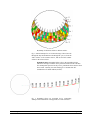
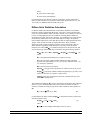
Viewshed calculation
Viewsheds are calculated for each cell of an input DEM. A viewshed is the
angular distribution of sky visibility versus obstruction. This is similar to
the view provided by upward-looking hemispherical (fisheye) photographs.
A viewshed is calculated by searching in a specified set of directions around
a location of interest (Fig. 1A), determining the maximum angle of sky
obstruction, sometimes referred to as effective horizon angle, in each
direction (Fig. 1B) (Dozier and Frew 1990). For other unsearched
directions, horizon angles are calculated using interpolation (Fig. 1C). Then
the horizon angles are converted into a hemispherical coordinate system, in
particular utilizing an equiangular hemispherical projection, which
represents a three-dimensional hemisphere of directions as a twodimensional grid (Fig. 1D). The resolution of the viewshed grid must be
sufficient to adeduately represent all sky directions, but small enough to
enable rapid calculations, e.g., 200 x 200 cells, 512 x 512 cells. Each grid
cell is assigned a value that corresponds with visible versus obstructed sky
directions. The grid cell location, row and column, corresponds to a zenith
angle θ (angle relative to the zenith) and an azimuth angle α (angle relative
to north) on the hemisphere of directions.
Solar Analyst Manual
What is the Solar Analyst? • 3
A) Directions for Horizon Angle Calculations
B) Calculation of Horizon Angles
C) Interpolation of Horizon Angles
4 • Contents
Solar Analyst Manual
D) Conversion to Hemispherical Coordiates
E) Resultant Viewshed
Fig 1. Calculation of the viewshed for one cell of a DEM. A)
Horizon angles are traced along a specified set of directions; B)
horizon angles are calculated for each direction; C) horizon angles
are interpolated for all directions; D) horizon angles are converted
to a hemispherical coordinate system; and E) the resulting
viewshed for a location represents which sky directions are visible
and which are obscured. Numbers represent the calculated horizon
angles.
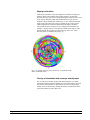
Sunmap calculation
The amount of direct solar radiation originating from each sky direction is
represented by creating a sunmap in the same hemispherical projection as
for the viewshed (Fig. 2). The sunmap consists of a raster representation
that specifies suntracks, the apparent position of the sun as it varies through
time. In particular, suntracks are represented by discrete sky sectors,
Solar Analyst Manual
What is the Solar Analyst? • 5
defined by sun position at intervals through the day and season (e.g., halfhour intervals through the day and month intervals through the season). The
position of the sun (zenith and azimuth angles) is calculated based on
latitude, day of year, and time of day using standard astronomical formulae
(modified version of Gates 1980). Zenith and azimuth angles are projected
into two-dimensional grids with the same resolution used for viewsheds.
Two sunmaps are created, one to represent periods between the winter
solstice and the summer solstice (December 22 to June 22) and the other to
represent periods between the summer solstice and the winter solstice (June
22 to December 22). Each sky sector of the sunmap is assigned a unique
identification number. For each sector, the associated time duration, the
azimuth and zenith at its centroid are calculated. This calculation also
accounts for partial sectors near the horizon.
A) Sunmap for Winter Solstice to Summer Solstice
6 • Contents
Solar Analyst Manual
B) Sunmap for Summer Solstice to Winter Solstice
Fig. 2. Annual sunmaps for 39o N latitude using 0.5 hour intervals
through the day and month intervals through the year, A) from the
winter solstice to the summer solstice, and B) from the summer
solstice to the winter solstice.
Penumbral effects: Penumbral effects refer to decreased direct beam
radiation at the edge of shadow due to partial obscuration of the solar disc.
For sunmaps that represent one day or less, penumbral effects must be taken
into account. Currently, the Solar Analyst use a constant solar disc
semidiameter of 0.00466 radians (0.2668o).
Fig. 3. Penumbral effects are accounted for by constructing
sunmaps with consideration of the apparent size of the solar disc.
Solar Analyst Manual
What is the Solar Analyst? • 7
Skymap calculation
Unlike direct insolation, which only originates from directions along the
suntrack, diffuse solar radiation can originate from any sky direction.
Skymaps are raster maps constructed by dividing the whole sky into a series
of sky sectors defined by zenith and azimuth divisions. Each sector is
assigned a unique identification number (Fig. 4). The zenith and azimuth
angles of the centroid of each sector are calculated. Sky sectors must be
small enough that the centroid zenith and azimuth angles reasonably
represent the direction of the sky sector in subsequent calculations. For
example, a skymap with 16 evenly spaced zenith divisions and 16 evenly
spaced azimuth divisions has sky sectors that represent 5.625o zenith
intervals and 22.5o azimuth intervals (Fig. 4).
Fig. 4. A skymap with sky sectors defined by 16 zenith divisions
and 16 azimuth divisions.
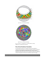
Overlay of viewsheds with sunmaps and skymaps
The viewshed is overlaid on skymap and sunmaps (Figure 5) to enable
calculation of diffuse and direct radiation received from each sky direction.
Gap fraction, the proportion of unobstructed sky area in each skymap or
sunmap sector, is calculated by dividing the number of unobstructed cells
by the total number of cells in that sector.
8 • Contents
Solar Analyst Manual
A) Overlay of Viewshed with Sunmap
B) Overlay of Viewshed with Skymap
Fig. 5. Overlay of a viewshed on A) a sunmap and B) a skymap.
Shaded areas are obstructed sky directions.
Direct Solar Radiation Calculation
For each sunmap sector that is not completely obstructed, solar radiation is
calculated based on gap fraction, sun position, atmospheric attenuation, and ground
receiving surface orientation of the intercepting surface. The Solar Analyst
implements a simple transmission model (Rich 1989, 1990, Pearcy 1989, Monteith
and Unsworth 1990, Gates 1980, List 1971), which starts with the solar constant and
accounts for atmospheric effects based on transmittivity and air mass depth.
Solar Analyst Manual
What is the Solar Analyst? • 9
Total direct insolation (Dirtot) for a ground location is the sum of the direct insolation
(Dir θ,α) from all sunmap sectors:
Dirtot = ΣDir θ,α
(1)
The direct insolation from the sunmap sector (Dir θ,α) with a centroid at zenith angle
θ and azimuth angle α is calculated using the following equation:
Dirθ,α = SConst * τm(θ) * SunDurθ,α * SunGapθ,α * cos(AngIn θ,α)
(2)
where:
SConst is the solar flux outside the atmosphere at the mean earth-sun
distance, know as solar constant. Estimates of the solar constant range from
1338 to 1368 WM-2. As a result of more precise measurements, the
Commission for Instruments and Methods of Observation in 1981 agreed to
adopt the World Radiation Center (WRC) solar constant (1367 WM-2), as is
used in the Solar Analyst. Solar constant fluctuates slightly, a few tenths of
a percentage over periods of years (Iqbal 1983), and this can be accounted
for by differences in the distance between the earth and sun from the mean
earth-sun distance;
τ is transmittivity of the atmosphere (averaged over all wavelengths) for the
shortest path (in the direction of the zenith);
m(θ) is the relative optical path length, measured as a proportion relative to
the zenith path length (see equation 3, below).
SunDurθ,α is the time duration represented by the sky sector. For most
sectors, it is equal to the day interval (e.g., a month) multiplied by the hour
interval (e.g., a half hour). For partial sectors (near the horizon), the
duration is calculated using spherical geometry;
SunGapθ,α is the gap fraction for the sunmap sector;
AngIn θ,α is the angle of incidence between the centroid of the sky sector
and the axis normal to the surface (see equation 4, below).
Relative optical length (m(θ)) is determined by the solar zenith angle and elevation
above sea level. For zenith angles less than 80o, it can be calculated using the
following equation:
m(θ) = EXP(-0. 000118 * Elev - 1. 638 * 10-9 * Elev2) /cos(θ)
(3)
where:
θ is the solar zenith angle;
Elev is elevation above sea level in meters.
The effect of surface orientation is accounted for by multiplying by the cosine of the
angle of incidence. Angle of incidence (AngInSky θ,α) between the intercepting
surface and a given sky sector with a centroid at zenith angle θ and azimuth angle α
is calculated using the following equation:
AngIn θ,α = acos[Cos(θ)*Cos(Gz)+Sin(θ)*Sin(Gz)*Cos(α-Ga)]
10 • Contents
(4)
Solar Analyst Manual
where:
Gz is the surface zenith angle;
Ga is the surface azimuth angle.
For zenith angles greater than 80o refraction is important. Various astronomical
tables provide corrections for refraction at zenith angles greater than 80o (e.g., List
1971, Table 137; Monteith and Unsworth 1990, p. 40).
Diffuse Solar Radiation Calculation
For diffuse radiation the uniform diffuse model and the standard overcast diffuse
model are typically implemented (Rich 1989, 1990, Pearcy 1989) with satisfactory
results. In a uniform diffuse model, sometimes referred to as a "uniform overcast sky
(UOC)" but often applied in clear sky conditions, incoming diffuse radiation is
assumed to be the same from all sky directions. In a standard overcast (SOC) diffuse
model, diffuse radiation flux varies with zenith angle according to an empirical
relation (Moon and Spencer 1942). Both these models are implemented in the Solar
Analyst. Other models can readily be implemented in the future, including
anisotropic models, based on assigning each sky sector an appropriate value for
diffuse radiation originating in that direction. For each sky sector, the diffuse
radiation at its centroid (Difθ,α) is calculated, integrated over the time interval, and
corrected by the gap fraction and angle of incidence using the following equation:
Difθ,α = Rglb * Pdif * Dur * SkyGapθ,α * Weight θ,α * cos(AngIn θ,α)
(5)
where:
Rglb is the global normal radiation (see equation 6 below);
Pdif is the proportion of global normal radiation flux that is diffused.
Typically it is approximately 0.2 for very clear sky conditions and 0. 7 for
very cloudy sky conditions;
Dur is the time interval for analysis;
SkyGapθ,α is the gap fraction (proportion of visible sky) for the sky sector;
Weight θ,α is proportion of diffuse radiation originating in a given sky sector
relative to all sectors (see equation 7 and 8, below);
AngIn θ,α is the angle of incidence between the centroid of the sky sector
and the intercepting surface.
The global normal radiation (Rglb) can be calculated by summing the direct radiation
from every sector (including obstructed sectors) without correction for angle of
incidence, and then correcting for proportion of direct radiation, which equals to 1Pdif:
Rglb = (SConst Σ (τm(θ) ) )/ (1 – Pdif)
(6)
For the uniform sky diffuse model, Weight θ,α is calculated as follows, based on the
derivation of Rich (1989):
Weight θ,α = (cosθ2 - cosθ1) / Divazi
(7)
where:
θ1and θ2 are the bounding zenith angles of the sky sector;
Solar Analyst Manual
What is the Solar Analyst? • 11
Divazi is the number of azimuthal divisions in the skymap.
For the standard overcast sky model, Weight θ,α is calculated as follows based on the
empirical model of Moon and Spencer (1942):
Weightθ,α = (2cosθ2 + cos2θ2 - 2cosθ1 - cos2θ1) / 4 * Divazi
(8)
Total diffuse solar radiation for the location (Diftot) is calculated as the sum of the
diffuse solar radiation (Dif θ,α) from all the skymap sectors:
Diftot = ΣDif θ,α
(9)
Global Solar Radiation Calculation
Global radiation (Globaltot) is calculated as the sum of direct and diffuse radiation of
all sectors.
Globaltot = Dirtot + Diftot
(10)
The above calculation of viewshed, overlay of viewshed on sunmaps and skymaps,
and calculation of direct, diffuse and global insolation are repeated for each location
on the topographic surface, thus producing insolation maps for an entire geographic
area.
12 • Contents
Solar Analyst Manual
Getting Started
System Requirements
Hardware: Pentium computers with a minimum of 32M RAM. The calculation also
requires a large disk space to store model results. The actual disk space required
depends on your input DEM size and output you need. Generally you should have
100M free space before running the model. More than a gigabyte of disk space can
be required for handling large DEMs and multiple outputs.
Operating System: MS Windows NT 4.x, Windows 95/98, or Windows 2000.
Software: ArcView 3.x and the Spatial Analyst extension.
Installation
Download the installation file, click the setup button, the installation wizard will
guide through the rest of the installation. The installation directory should be where
ArcView is installed, e.g. c:\esri\av_gis30\arcview.
The installation program will install SolarExt.Avx to the ext32 directory, and several
DLLs to the bin32 directory. These files will be removed when the Solar Analyst is
uninstalled.
Solar Analyst Manual
Getting Started • 13
Tutorial
Preparing the Sample Data
First, you will download the sample data (size <350 KB compressed), set up a
working directory, extract the data, load the Solar Analyst extension, and load the
data into ArcView.
Download Sample Data
Download the sample data from the following web site:
http://www.hemisoft.com/download/solaranalyst/samples.exe.
Make a directory (e.g., d:\samples), and unzip the sample data to this directory. The
following data will be extracted.
Dem (DEM grid),
Demm (mask grid),
Dema (aspect grid),
Dems (slope grid),
Pntcov (point coverage), and
Pntxy.txt (X/Y coordinate file with slope and aspect).
Create an Output Directory
This tutorial will generate many output files. It would be good to create an output
directory (e.g. d:\tutorial) and store output files in this directory. Be sure that at least
10 Mbytes is available on the disk where the directory is located.
Load the Solar Analyst
Start ArcView, and then choose the Extensions… dialog from the File menu. Check
Solar Analyst; then click OK. Start a new view window (by default, the name of the
view is “view1”. The menu Solar will appear in the view menu bar, and three new
icons will appear (a button and two tools).
14 • Contents
Solar Analyst Manual
Load Sample Data
Add the following sample data to view1: Dem as a grid theme and Pntcov as a point
theme. Make Dem the active theme. Observe that the Solar Analyst tools are now
enabled.
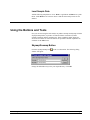
Using the Buttons and Tools
Now you can start using the Solar Analyst to produce sunmaps and skymaps with the
skymap/sunmap button, to produce viewsheds with the viewshed tool, and to
calculate insolation with the insolation tool. These capabilities enable interactive
selection of locations for which calculations are performed. Further capabilities are
available via the Solar menu.
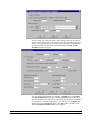
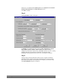
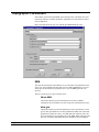
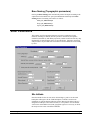
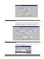
Skymap/Sunmap Button
Click the skymap/sunmap icon
window will appear.
on the view button bar. The following dialog
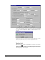
Change the default directory to the your output directory. Click OK.
Solar Analyst Manual
Tutorial • 15
You may change the default parameters. Change the sky size to 400 and the latitude
to 45. Change the time configuration to Whole year with monthly interval. Then
click OK.
Click Yes. You will see a view named “Viewshed, sunmap and skymap” is created
and the skymaps and sunmaps you just created are displayed in this view.
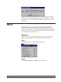
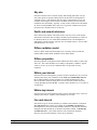
Viewshed tool
Make View1 the active window, and make dem the active theme. Observe that the
viewshed tool icon
on the view tool bar is enabled. Click the viewshed tool icon.
Then choose a location for calculating a viewshed by clicking anywhere in view1.
The following dialog window will appear.
16 • Contents
Solar Analyst Manual
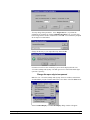
You may change these parameters. Leave height offset as 0, to perform the
calculation for ground level. Change calculation directions to 64, to specify that
horizon angle will be traced in 64 directions. Click OK. You will then be prompted
for the output viewshed names:
Change the directory to your output directory and click OK.
Click Yes. You will see the viewshed you just created is displayed in the view
“Viewshed, sunmap and skymap”. The dark green area is obstructed and the light
cyan area is open sky.
Change the open sky to transparent
Make the view “Viewshed, sunmap and skymap” the active window, and click the
viewshed theme you just created to make it the active theme. Select the Solar menu:
Select Viewshed Display. The Viewshed display dialog window will appear:
Solar Analyst Manual
Tutorial • 17
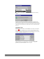
Select Change viewshed themes. You will then be prompted for the following
question:
Click Yes. The open sky in the viewshed is now displayed as transparent. The
sunmap will now be visible in the open sky directions. Note which part of the sun
track is blocked and which part is open. Check off the sunmaps so that the skymap is
visible in the open sky directions. Note which part of the sky is blocked and which
part is not.
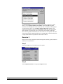
Insolation Tool
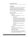
Make View1 the active window, and make dem the current theme. The insolation
tool icon
will be enabled in the view tool bar. Click the insolation tool icon.
Then select a location for which insolation will be calculated by clicking anywhere
in view1. The Insolation output files dialog window will appear:
Change the directory to your output directory. Click OK. The Topographic
parameters for location calculation window will appear:
18 • Contents
Solar Analyst Manual
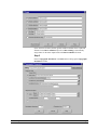
You may change any of these parameters. Slope and aspect can be given constant
values or can be derived from a grid. Choose the slope file dems and the aspect file
dema in your sample data directory. Note that if the slope and aspects grids did not
exist, they would be automatically created from the DEM. Click OK. The Sky
Parameters window will appear:
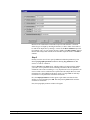
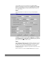
You may change these parameters. For example, set latitude to 45. Select Whole
year with monthly interval. Thencheck the For each interval option. This option
will cause insolation to be calculated for each month, since the interval is monthly. If
we had preferred to calculate hourly patterns, we could have selected Within day
and checked the For each interval option. Click OK to initiate calculations. The
following Insolation calculation dialog box will appear:
Solar Analyst Manual
Tutorial • 19
Click Yes. The monthly insolation patterns will be displayed as tables and charts.
Enlarge each of the charts and inspect your results. (Note: Limitations of ArcView
may only permit view of part of the data, although all of the data is present in the
output files.)
Menus
The Solar menu provides more capabilities than the buttons and toolbars. The
buttons and toolbars are only useful for interactive calculations for selected
locations. The Solar menu enables batch calculation, including insolation maps and
calculations for many locations. This tutorial includes three exercises to familiarize
users with the menus of the Solar Analyst.
Exercise 1
In this exercise the user calculates insolation (direct, diffuse, global, and direct
duration), skymap/sunmaps, and viewsheds for locations in a point theme.
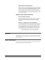
Step 1
Select the Solar menu. The following choices will appear.
Step 2
Select Output Parameters. The Output window will appear:
20 • Contents
Solar Analyst Manual
Results will be calculated for each kind of output for which the box is checked.
Select all types of output by checking all the boxes, as above. Enter a base name to
be used for all output files by entering a a name for the direct radiation output file.
For example, enter d:\{your_output_directory}\raddir. Click Base Naming. Observe
that the Solar Analyst fills in names for all the other output file names. Click OK to
continue.
Step 3
In many cases the user will now specify additional calculation paramters by first
choosing topographic parameters and then choosing sky parameters. In this
exercise we will use a shortcut.
Choose !Execute in the Solar menu. A dialog window will appear asking whether
you wish to review parameters before initiating calculations. Because insolation
calculations can be time consuming, it is very important to be sure all parameters are
correct. In this exercise calculations are rapid because the sample data set is small.
Calculation for a large DEM can take hours, and a very large DEM can take days.
Click Yes to review paramaters and initiate calculations.
First, the output parameters window appears again. Make sure that all of the
settings are correct and then press OK. Note that pressing Cancel will cancel the
execution of calculations.
Next, the topographic parameter window will appear:
Solar Analyst Manual
Tutorial • 21
The DEM drop box, selected by clicking the small downward arrow, enables choice
of input DEM theme. In our case there is only one choice, the sample DEM theme in
view1.
Click Base Naming and note how this causes the mask, slope, and aspect input grids
to use the same base name as the DEM.
Observe that Whole DEM and Mask Grid are disabled because you previously
checked viewshed output in the output parameters window, and because viewshed
can only be calculated for specific locations. It would not be practical to store
viewsheds for all locations in a DEM, although they are all calculated when
producing insolation maps.
Select Locations from a point theme. The point theme pntcov will appear. If
multiple points themes are available, the desired theme should be selected with the
drop box.
The Slope and Aspect dialog enables specification of surface orientation either from
a Grid or from a user-specified Constant value. Select Grids. Note that the slope
and aspect grids were included with the sample data.
Alternatively, the same location data could be entered from a text file that contains
map coordinates, slope, and aspect values, as follows:
x,y,slope,aspect
22 • Contents
0.3255412E+06,
0.4314769E+07,10,330
0.3251693E+06
0.4313907E+07,20,270
0.3258740E+06;
0.4313134E+07;20,90
0.3258251E+06
0.4314182E+07;15,180
Solar Analyst Manual
In this case, we would choose Locations by X/Y as the Analysis Area and ASCII
format in the location file as the Slope and Aspect source.
Click OK to continue.
Step 4
The sky parameter window will appear:
Set latitude to 39 and sky size to 400. Select the Time configuration as Special
Days: summer solstice / equinox / winter solstice. This choice performs
calculations for these three “special” days. Click OK to continue. As before, clicking
Cancel would cancel the execution of calculations. Now that the output,
topographic, and sky parameters have been review, calculations are initiated.
Step 5
The Solar Analyst will take different amounts of time to complete calculations
depending upon the computer being used. Calculations for this exercise typically
take one to several minutes. Once calculations are complete, you will hear a beep
and a Results Display dialog box will appear:
Solar Analyst Manual
Tutorial • 23
The Results Display permits choice of which output results to display as a table,
chart, or view. Highlight Global and Viewshed. Then press OK. The global
insolation will be displayed in a table and a chart. The viewsheds will be displayed
as separate themes in the view viewshed, sunmap and skymap. Examine your
results. You can observe four new viewshed themes in the view, four curves in the
chart, and four rows in the table, one for each of the four locations in the point
theme. For the global insolation table, the order of the rows corresponds to the order
of the location labels in view1. Similarly, the viewshed grids use the base name plus
a unique number that corresponds to the label order in view1.
Exercise 2
In this exercise the user calculates insolation maps (direct, diffuse, global, and direct
duration) for a specified area.
Step 1
Choose the Solar menu. The following choices appear:
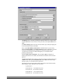
Step 2
Select Output Parameters to bring up the Output window:
24 • Contents
Solar Analyst Manual
Check the boxes for direct, diffuse, global, and direct duration. Enter a path and
filename for the Direct radiation output. Press Base Naming to automatically
assign names for the other output based on the Direct radiation file name.
Step 3
Choose Topographic Parameters in the Solar menu to bring up the Topographic
Parameters window:
Solar Analyst Manual
Tutorial • 25
Verify that dem is specified as the input DEM. Then click Base Naming to
automatically assign names for other input files. For Analysis Area, choose Mask
Grid and verify that demm is the mask grid. For Slope and Aspect choose Grids
and verify that dems and dema are the slope and aspect grid names, respectively.
Choose OK to continue.
Step 4
Choose Sky Parameters in the Solar menu to bring up the Sky Parameters
window:
Set latitude to 39 and sky size to 200. For Time Configuration select Within day
and set Day (Julian day) to 188, Start Time to 0, and End Time to 24 , . Be sure the
box For each Interval is not checked. If this box is checked, a separate grid will be
produced for each 0.5 hour. Choose OK to continue.
Step 5
Choose !Execute in the Solar menu to initiate calculations. Click Yes to review the
Output, Topographic, and Sky Parameters. For each of the parameter windows
press OK. After you press OK for the Sky Parameters, calculations will start. It
may require several minutes to complete calculations for the sample DEM,
depending upon the computer configuration. Larger DEMs can require hours or days
to complete calculations.
When the calculations are complete, the Display Results dialog box will appear:
26 • Contents
Solar Analyst Manual
Highlight Global and Duration and Click OK. The results will be displayed in
view1 using the predefined classification method and shade color ramp. Inspect the
maps to see how annual global insolation and direct duration differ according to
topographic position.
Solar Analyst Manual
Tutorial • 27
Menu References
Solar menu
The Solar Analyst adds a Solar menu to the view menu bar. This menu provides
access to an array of solar modeling capabilities.
Output parameters
This window enables the user to specify details of calculations to be performed and
output files. Check each type of output to be calculated and specify a filename
(including directory) where results are to be placed. Base Naming enables automatic
naming based on the direct solar radiation name. Explanations of each output choice
are provided below. Important notes are provided at the end of this section and
should be read carefully by users.
28 • Contents
Solar Analyst Manual
Direct solar radiation:
Check this box to output direct radiation files. This choice specifies that direct
incoming solar radiation will be calculated. The output has units of WH/m2. The
specified file name is used as the base file name for other outputs (see Base
Naming). Output format can be either grid or ASCII text.
Diffuse solar radiation
Check this box to output diffuse radiation files. This choice specifies that diffuse
incoming solar radiation will be calculated. The output has units of WH/m2. When
this choice is selected, direct solar radiation output is also automatically selected.
Output format can be either grid or ASCII text.
Global solar radiation
Check this box to output global radiation files. This choice specifies that global
(direct + diffuse) incoming solar radiation will be calculated. The output has units of
WH/m2. When this choice is selected, direct and diffuse solar radiation outputs are
also automatically selected. Output format can be either grid or ASCII text.
Direct radiation duration
Check this box to output direct radiation duration files. This choice specifies that the
duration of direct incoming solar radiation will be calculated. The output has units of
hours. When this choice is selected, direct solar radiation is also automatically
selected. Output format can be either grid or ASCII text.
Output Formats:
Outputs for direct, diffuse, global, and direct duration all use either grid or ASCII
text formats:
•
Solar Analyst Manual
ESRI Grid format when calculating for whole grids or masked areas.
Menu References • 29
The program automatically adds numbers to the output name(s). For example,
when using an input file with the name myfile, the output files will be named
myfile0, myfile1, myfile2… The number of output grids depends on settings in
the Solar parameters window, in particular, the for each interval checkbox.
•
¾
If for each interval is not checked: the actual output is myfile0, which is the
total direct radiation for the calculated duration.
¾
If for each interval is checked: the actual outputs are myfile0, myfile1,
myfile2… Each grid stores the direct radiation for each time interval (hour
of day interval when duration is less than one day, or day of year interval
when duration is longer than one day).
In ASCII text format when calculating for selected locations. The actual output
file is named as myfile.txt. Its format depends on the for each interval checkbox
in the Solar Parameters window.
¾
If for each interval is not checked, the output ASCII file format is as
follows:
row, column, value
…
where row and column specify the location of the selected cell and value is
the radiation or duration value for the whole interval specified in the solar
parameter window.
¾
If the for each interval checkbox is checked, the output ASCII file format is as
follows:
row, column, value0, value1, value2…
…
where value0, value1, value2,… indicate radiation or duration values for
each time interval (hour of day interval when duration is less than one day,
or day of year interval when duration is longer than one day).
Skymap and Sunmap
Check this box to output skymap and sunmap files. This choice specifies that the
skymap and sunmap will be output in ESRI Grid format. The resolution of these
grids is specified in the Solar Parameters window.
Skymap: Only one grid is generated for the skymap.
Sunmap: One or two sunmap grids may be generated, depending upon whether the
interval includes overlapping sun positions for different times of year. A number is
attached to the name of each sunmap (e.g., sunmap0 and sunmap01).
Viewshed
Check this box to output viewshed files. This choice enables calculation of
viewsheds for specified locations. A list of locations for calculation can be specified
in the Topographic Parameters window by X, Y coordinates or by cell row and
column. The output is in ESRI Grid format at the same resolution as the skymap and
sunmap.
30 • Contents
Solar Analyst Manual
Base Naming (output)
Press the Base–naming button to name all outputs according to the output name for
the direct insolation calculation. First check the direct radiation output, next specify a
name, and then press the Base–naming button. (If direct radiation is not a desired
output, it can be checked off again after base naming has been performed.) The
naming convention is as follows:
Direct solar radiation: {basename}dir
Diffuse solar radiation: {basename}dif
Global solar radiation: {basename}glb
Direct radiation duration: {basename}dur
Skymap: {basename}sky
Sunmap: {basename}sun
Viewshed: {basename}v
Important Notes (output)
Base Names and Actual Output File Names
All names specified in the output parameter windows are base names. They
are not the actual output file names. The actual file names add number
indices to the base names. ArcView decides the number indices by avoiding
file overwriting. For example, if the base name for direct radiation is raddir
and a grid with a name raddir0 already exists, the next output for the direct
solar radiation grid will be raddir1. You may wish to record a log of output
to keep track of file contents while using the Solar Analyst.
By using base naming, users do not have to specify output names for each
calculation. Protection against overwriting files also prevents data loss and
crashes of ArcView.
Directory Creation
The Solar Analyst creates output grids or ASCII files, but it does not create
the directories to contain these grids or ASCII files. For example, if you set
your output direct solar radiation grid as d:\my_directory\insolation\raddir,
then the directory d:\my_directory\insolation must first be created before
you can start the calculations. If the directory does not exist, the Solar
Analyst report an error and calculations will not proceed.
No Float Grid
Output grids (including direct, diffuse, global, and direct duration) are all of
integer type (because of a limit with creating float grids using C++). For
calculations of instantaneous time periods, values are small, so results are
multiplied by 100 to retain accuracy These grids should be divided by 100
to obtain their float values:
e.g., Grid: gridinst = float(outgrid / 100.0)
Solar Analyst Manual
Menu References • 31
Topographic Parameters
This window specifies the input DEM, slope and aspect files, calculation area, and
parameters related to viewshed calculations. Explanations of each parameter choice
are provided below.
Before selecting this menu, the view with the input DEM should be active.
DEM
This specifies the filename of the DEM to use for calculation. All grid themes in the
active view will be added to the drop-down list of available DEM choices. In cases
where there are more than one grid in the active view, the DEM grid must to be
selected.
The user can specify five types of analysis areas:
Whole DEM
Choose this option to perform calculations for all cells of a DEM.
Calculations are performed for all cells except cells with NODATA values.
Mask grid
Choose this option to perform calculations for an area specified by a mask
grid. A mask grid should be an existing ESRI Grid. When cells of the mask
grid that have NODATA values, viewsheds and solar radiation values will
not be calculated for corresponding cells in the DEM. When mask grid cells
have any value other than NODATA, then calculations are performed for
32 • Contents
Solar Analyst Manual
corresponding cells. Note that the entire DEM is still used for calculating
viewsheds.
Locations from a point theme
Choose this option to perform calculations for a list of locations in a point
theme. The theme can be an ARC/INFO coverage or an ArcView shape file.
If particular locations have been selected in ArcView, then calculations will
be performed only for those locations.
Locations by row and column
Choose this option to perform calculations for a list of locations specified in
a row/column file. The row/column file should be an existing ASCII text
file. Each line in the file should contain a row and column pair separated by
space(s), comma(s), or semicolon(s). Blank lines and headlines will be
filtered out when the file is read. The following is an example:
Row, col
8, 6
200; 500
700 1000
Locations by x and y coordinates
Choose this option to perform calculations for a list of locations specified in
an X,Y coordinate file. The X,Y coordinate file should be an existing ASCII
text file. Each line in the file should contain an X,Y pair separated by
space(s), or comma(s), or semicolons (s). Blank lines and headlines will be
filtered out when the file is read. The following is an example:
X, Y
12989.8; 28934.5
12345.567, 89453.213
700.456 1000.432
Location height offset
Enter the height offset appropriate for your calculations (default = 0). This value
specifies the height (in meters) above the DEM surface for which calculations are to
be performed. The same height offset will be applied to all locations specified in the
X,Y coordinate file or row/column file.
For example, weather station sensors and solar powered devices are usually
positioned at a height above ground level. Height offsets can make significant
differences for viewshed and insolation calculations.
Slope and aspect
Specify the names (along with the directories) of the slope and aspect grids to be
used for calculations. The user can specify three types of slope and aspect
information:
Solar Analyst Manual
Menu References • 33
Grids
Slope and aspect are derived from slope and aspect grids. Specify the names
for the slope and aspect grids. Typically, these are calculated using either
the ARC/INFO GRID slope and aspect commands, or using the Derive
Slope and Derive Aspect menu choices of the Spatial Analyst extension of
ArcView. Note, when using ArcView, the resultant slope and aspect grids
are placed in a temporary directory (usually c:\temp). Slope and aspect grids
can also be constructed by users according to field measurements or other
rules. If the specified slope and aspect grids do not exist, the Solar Analyst
will automatically create them.
Constant values
Specify constant values for slope and aspect. For example, users need use
slope 0 and aspect 0 corresponding to solar radiation sensors, or other
orientations for surfaces such as leaves.
ASCII format in the location file
Specify slope and aspect in the location files (X/Y or R/C). The location file
should be an existing ASCII text file. Each line in the file should contain a
row/column or a x/y along with the slope and aspect. The values in each
line should be separated by space(s), comma(s), or semicolon(s). Blank
lines and headlines will be filtered out when the file is read. The following
is an example:
Row, col, slope, aspect
8, 6, 15, 20
200; 500, 40,180
700 1000,32;275
The following is another example:
X, Y
12989.8; 28934.5, 15, 20
12345.567, 89453.213, 40,180
700.456 1000.432; 32;275
Directions
Enter the number of azimuth directions used when calculating viewsheds. Because
the viewshed calculation is highly intensive, horizon angles are only traced for the
number of directions specified. Valid values must be multiples of 8 (8, 16, 24, 32…).
Typically, a value of 8 or 16 is adequate for areas with gentle topography, whereas a
value of 32 is adequate for complex topography.
Elevation unit
Choose the units of measurement (meters, feet, etc.) of the input DEM. The Solar
Analyst automatically converts the DEM elevation values into meters for calculation
of air mass (the atmospheric path through which solar radiation travels).
34 • Contents
Solar Analyst Manual
Base Naming (Topographic parameters)
Pressing the Base Naming button automatically names all outputs according to the
output name for the DEM. First specify the DEM name and then press the Base
Naming button. The naming convention is as follows:
Mask grid: {DEM name}m
Slope grid: {DEM name}s
Aspect grid: {DEM name}a
Solar Parameters
This window specifies important parameters relevant to calculation of solar
radiation, including site latitude, the time period for calculations, atmospheric
conditions (transmittivity and diffuse proportion), and the resolution of the sky map.
Explanations of each parameter choice are provided below. Important concerning
solar parameters are provided at the end of this section and should be read carefully
by users.
Site latitude
Enter the latitude for the site area (units: decimal degree, positive for the north
hemisphere and negative for the south hemisphere). Latitude is used in such
calculations as solar declination and solar position. Because The Solar Analyst is
designed for landscape scales and local scales, it is acceptable to use one latitude
value for the whole DEM. For broader geographic regions it is necessary to divide
the study area into zones with different latitudes.
Solar Analyst Manual
Menu References • 35
Sky size
Enter the resolution of the viewshed, skymap, and sunmap grids (units: cells per
side). These grids are upward–looking maps of sky direction in a hemispherical
coordinate system. Note that these grids are square (equal numbers of rows and
columns). Increasing this value increases calculation accuracy but also increases
calculation time considerably. Typically, a value of 200 is sufficient for calculations
for whole or masked DEMs, and a value of 512 is good for calculations at specific
locations where calculation time is not an issue.
Zenith and azimuth divisions
Enter values for the number of divisions used to create sky sectors in the skymap.
The number of divisions does not change calculation speed. Satisfactory results can
be obtained with as few as 8 zenith and 8 azimuth divisions. The hemispherical
photography scientific literature typically uses 18 zenith divisions (5° sectors) and 8
azimuth divisions (45° sectors).
Diffuse radiation model
Choose a diffuse model from the dropdown list. Currently, choices include the
uniform diffuse model and the standard overcast diffuse model.
Diffuse proportion
Enter the proportion of the global normal radiation flux that is diffuse. Values range
from 0 to 1. This value should be set according to atmospheric conditions. Typical
values are 0.2 for very clear sky conditions and 0.3 for generally clear sky
conditions.
Within year interval
Enter the time interval through the year that is used for calculation of sky sectors for
sunmaps (units: days). For calculations of the whole year with monthly interval,
this is disabled and the program internally uses calendar month intervals. Day
interval should be usually be larger than 3 because sun tracks within 3 days may
overlap depending upon the sky size. Typically values should be set to 7 (weekly) or
14 (biweekly).
Within day interval
Enter the time interval through the day that is used for calculation of sky sectors for
sunmaps (units: hours). Typically values should be set to 1 hour.
For each interval
This check box gives users the flexibility to calculate total insolation or insolation
For each interval. For example, for multiple day and Within year interval of 7,
checking this box will create weekly insolation, otherwise, only the total insolation
during the start day and end day is calculated. In another example, for Within day
and Hour interval of 1, check this check box will create hourly insolation,
otherwise, only the total insolation over the day is calculated.
36 • Contents
Solar Analyst Manual
Direct radiation model
Choose a direct model from the dropdown list. Currently, only a simple transmission
model is available.
Transmittivity
Enter a transmittivity value to be used in calculations. This value is the transmittivity
of the atmosphere (averaged over all wavelengths), expressed as the proportion of
exoatmospheric radiation transmitted as direct radiation along the shortest
atmospheric path (i.e., from the direction of the zenith). Values range from 0 (no
transmission) to 1 (all transmission). Because The Solar Analyst corrects for
elevation effects, transmittivity should always be given for sea level. Typical values
are 0.6 or 0.7 for very clear sky conditions and 0.5 for generally clear sky. Note that
transmittivity has an inverse relation with the diffuse proportion parameter.
Time configuration
This group of choices specifies the time periods used for calculations.
Within day
Choose this option to perform calculations for a specified time period
within a day. Enter start time and end time.
Instantaneous
When the start time and the end time is the same, instantaneous
insolation will be calculated. Note that the current implementation
outputs integer grids, with values multiplied by 100 to retain
calculation accuracy for direct, diffuse, global, and duration grids.
This implementation was necessary because of limitations of the
ArcView GRIDIO library, whereby float grid can not be generated
using C++. Instantaneous ouput grids (including direct, diffuse,
global, and duration) should be divided by 100 to obtain their
correct float values:
Grid: instantaneousgrid = float(calculatedgrid / 100.0)
Whole day
When the start time is before the sunrise and the end time is after
the sunset, insolation will be calculated for the whole day.
Special Days
Choose this option to calculation insolation for summer
solstice/equinox/winter solstice days. Note that the For each interval
option is disabled for the latter choice.
Multi day User Specified
Choose this option to perform calculations for a specific multiple day period
within a year. Specify the start day, start year, end day, within year
interval, and within day interval. When end day is smaller than start day,
the end day is considered to be in the following year.
Solar Analyst Manual
Menu References • 37
Whole year with monthly interval
Choose this option to perform calculations for an entire year using monthly
intervals for calculations. If the For each interval option is checked, then
output files will be created for each month. Otherwise, output files will be
created for the whole year. Note that The Solar Analyst uses calendar
months, with different number of days per month. Users should use caution
when comparing insolation for months that have different numbers of days
(e.g., January vs. February).
Important Notes (Solar parameters)
For each interval checkbox
This parameter changes the numbers of output files, names of output files,
and formats of output files. In turn, it changes the disk space required.
Always verify that sufficient disk space is available before initiating
calculations.
Results for instantaneous time configuration
The current implementation outputs integer grids, with values multiplied by
100 to retain calculation accuracy for direct, diffuse, global, and duration
grids. This implementation was necessary because of limitations of the
ArcView GRIDIO library, whereby float grid can not be generated using
C++. Instantaneous output grids (including direct, diffuse, global, and
duration) should be divided by 100 to obtain their correct float values:
Grid: instantaneousgrid = float(calculatedgrid / 100.0)
Execute
The !Execute choice initiates calculations. First, users are prompted to confirm the
output, topographic, and sky parameters. Next, calculations are performed. Finally,
results are displayed.
Date Conversion
This window converts calendar day to julian day. This window is also available in
the sky parameter dialog by clicking the day buttons.
38 • Contents
Solar Analyst Manual
Time Conversion
This window converts local solar time (HMS) or local standard time to local solar
time (decimal hours). When converting local standard time to local solar time, the
program accounts for equation of time. This window is also available in the sky
parameter dialog by clicking the time (start time and end time) buttons.
Viewshed Display
This choice allows users to display viewshed grids using a predefined legend. It
brings up the following window.
Solar Analyst Manual
Menu References • 39
The choice “add viewshed grids” allows users to add viewshed grids, while “change
viewshed themes” changes the legends of the current active themes in the current
views. The latter one allows users to specify whether or not open sky in the
viewsheds be transparent or not.
Sky/Sun Map Display
This choice allows users to display viewshed grids using a predefined legend. It
brings up the following window.
The choice “add viewshed grids” allows user to add viewshed grids, while “change
viewshed themes” changes the legends of the current active themes in the current
views.
Insolation Display
This choice enables users to display calculated direct/diffuse/global insolation and
direct radiation duration. It brings up the following window.
The choice “Display grids” allows user to add insolation/duration grids into the
current view using a predefined legend. The legend classifies the grids into 14
classes, using a combination of natural interval and linear stretch. The grids are
displayed using a color ramp from blue to green to red to yellow to white. Note:
when the grids are large and have too many unique values, their VATs are not built
automatically when the grids are created. Without the VATs, these grids can not be
displayed using the predefined legend. In such cases, the program builds the VATs
for such grids, the resultant VATs can be large (up to several hundred kilobytes or
more). The choice “Display text files” allows user to add the insolation/duration text
files as tables and charts.
40 • Contents
Solar Analyst Manual
Error Codes
Error Codes
Error codes of generated by the Solar Analyst are listed below. They can help user understand the
problems encountered while using the Solar Analyst. These codes can also help users report bugs.
1 Solar.cpp: Can not initialize GRID environment
2 Sky.cpp: Latitude out of range
100 Solar.cpp: Can not open file of horizon zeniths
110 Solar.cpp: Too few directions
111 Solar.cpp: Can not allocate memory for storing horizon zenith angles
112 Solar.cpp: Can not allocate memory for reading the DEM grid
113 Solar.cpp: Can not set the DEM grid IO mode to REGIONIO
114 Solar.cpp: Error reading the DEM grid into memory
115 Solar.cpp: Can not allocate memory for reading the DEM grid
116 Solar.cpp: Error reading the DEM grid into memory
131 Solar.cpp: Can not open input grid
132 Solar.cpp: Can not get grid boundary
133 Solar.cpp: Can not set grid access window
134 Solar.cpp: Can not open file for horizon zeniths
140 Solar.cpp: Viewshed calculation is designed for location calculation mode.
150 Solar.cpp: Row and column do not make pairs or are out of DEM boundary
151 Solar.cpp: Row and column do not make pairs or are out of DEM boundary
160 Solar.cpp: Mask grid does not exist
163 Solar.cpp: Can not read mask grid boundary
163 Solar.cpp: Mask grid and DEM grid do not overlap
164 Solar.cpp: Can not set access window for mask grid
170 Solar.cpp: Output viewshed file name is blank
172 Solar.cpp: Output global radiation file name can not be blank
173 Solar.cpp: Output direction radiation file name can not be blank
174 Solar.cpp: Output diffuse radiation file name can not be blank
180 Solar.cpp: Input slope grid does not exist
Solar Analyst Manual
Error Codes • 41
181 Solar.cpp: Input aspect grid does not exist
182 Solar.cpp: Can not open slope grid
183 Solar.cpp: slope grid is not float
184 Solar.cpp: Can not open aspect grid
185 Solar.cpp: Aspect grid is not float
186 Solar.cpp: Can not get slope grid boundary
187 Solar.cpp: Can not get aspect grid boundary
188 Solar.cpp: Slope and aspect grids do not overlap DEM grid
189 Solar.cpp: Slope and aspect grids do not overlap mask grid
190 Solar.cpp: Can not set the access window for slope and aspect grids
191 Solar.cpp: Can not set the access window for slope and aspect grids
200 Solar.cpp: Number of output files less than 1
210 Solar.cpp: Can not delete the existing grid file.
211 Solar.cpp: Can not create output grid file.
212 Solar.cpp: Can not set access window.
220 Solar.cpp: Can not open output direct radiation file for pixel calculation
221 Solar.cpp: Can not open output diffuse radiation file for pixel calculation
222 Solar.cpp: Can not open output global radiation file for pixel calculation
223 Solar.cpp: Can not open output direct duration radiation file for pixel calculation
231 Solar.cpp: wrong output file name for direct radiation
304 Sky.cpp: Can not allocate memory for diffuse sky
305 Sky.cpp: Can not allocate memory to store the skymap sector information
306 Sky.cpp: Can not allocate memory to store total pixels for each skymap sector
307 Sky.cpp: Can not allocate memory to store open pixels for each skymap sector
308 Sky.cpp: Can not allocate memory to store gap fractions for skymap
310 Sky.cpp: Can not delete the existing grid file.
311 Sky.cpp: Can not create output grid file.
312 Sky.cpp: Can not set access window.
313 Sky.cpp: Can not delete the existing grid file.
314 Sky.cpp: Can not create output grid file.
315 Sky.cpp: Can not set access window.
330 Sky.cpp: Sky size too small
331 Sky.cpp: Can not allocate memory for sky fill
332 Sky.cpp: Can not allocate memory for viewshed sky
339 Sky.cpp: Zenith divisions are not correct
340 Sky.cpp: File name for sky map and sun map can not be blank.
341 Sky.cpp: Night, no sun
42 • Contents
Solar Analyst Manual
342 Sky.cpp: Zenith sector is not correct
351 Sky.cpp: Can not allocate memory to store sunmap sector information
352 Sky.cpp: Can not allocate memory to store sunmap sector pixels
353 Sky.cpp: Can not allocate memory to store sunmap sector open pixels
354 Sky.cpp: Can not allocate memory to store sunmap sector gap fractions
355 Sky.cpp: Can not allocate memory for sunmap I
356 Sky.cpp: Can not allocate memory for sunmap II
360 Sky.cpp: Can not open file
370 Sky.cpp: End hour is smaller than start hour
371 Sky.cpp: All night
372 Sky.cpp: night, no sun
382 Sky.cpp: Time interval can not be negative
383 Sky.cpp: Not suit for single day calculation
391 Sky.cpp: Diffuse proportion is out of range (0–1)
392 Sky.cpp: Diffuse proportion is out of range (0–1)
400 Segment.cpp: Can not allocate memory for flood–fill buffer
401 Sky.cpp: Sky transmittivity is out of rang (0–1)
430 Solar.cpp: Input grid does not exist
701 Solar.cpp Invalidate calculation area
702 Solar.cpp Point Array full
703 Solar.cpp Point Array full
705 Solar.cpp Slope and aspect values are out of range
706 Solar.cpp Number of calculation directions can not be negative
707 Solar.cpp invalidate elevation unit
708 Solar.cpp Latitude is out of range
709 Solar.cpp Sky size can not be negative
710 Solar.cpp Time configuration for within day is out of range
711 Solar.cpp Time configuration for multiday is out of range
712 Solar.cpp Hour interval is out of range
713 Solar.cpp Hour interval is out of range
714 Solar.cpp Zenith and azimuth divisions are out of range
715 Solar.cpp Time has not been configured
720 Solar.cpp "No output configured, can not continue"
721 Solar.cpp Viewshed calculation is for location calculation only
777 Solar.cpp Number of points can not be negative
778 Solar.cpp Point buffer has not been allocated
779 Solar.cpp Slope and aspect buffer has not been allocated
Solar Analyst Manual
Error Codes • 43
788 Solar.cpp Transmittivity is out of range (0-1)
789 Solar.cpp diffuse proportion is out of range (0-1)
801 Sun.cpp: Latitude not set yet for CSun
902 Sky.cpp: Can not allocate memory to store skymap duration
More Solar Radiation Models
TopoView
What is TopoView?
TopoView is a spatial solar radiation model that uses digital elevation models
(DEMs) for input and produces a variety of outputs, including accurate incoming
solar radiation (insolation) maps.
TopoView generates upward-looking hemispherical viewsheds, in essence producing
the equivalent of an upward looking hemispherical photograph for every location on
a DEM. The hemispherical viewsheds are used to calculate the insolation for each
location and to produce accurate insolation maps. TopoView can calculate insolation
integrated for any time period. It accounts for site latitude and elevation, surface
orientation, shadows cast by surrounding topography, daily and seasonal shifts in
solar angle, and atmospheric attenuation. See the TopoView Manual to learn more.
TopoView is currently available for MS Windows NT4.0 and MS Windows 95/98.
TopoView Features
Versatile output: calculates direct, diffuse, global radiation; direct radiation
duration; sunmaps and skymaps; and viewsheds;
Simple input: requires only DEM, atmospheric transmittivity, and diffuse
proportion (latter two parameters calculated from nearby weather stations or using
typical values);
Flexibility:
- calculates insolation for any specified period (instantaneous, daily, monthly,
weekly ...);
- calculates insolation for any region (whole DEM, restricted areas, or point
locations);
44 • Contents
Solar Analyst Manual
- allows specification of receiving surface orientation (from DEM, field survey, or
orientations of surfaces such as sensors or leaves) and height offsets for ground
features;
Fast and accurate calculations: uses an advanced viewshed algorithm for
calculations; accounts for viewshed (sky obstruction by near-ground features),
surface orientation, elevation, and atmospheric conditions; calculation engine
implemented in C++ library format and dynamically loaded.
TopoView vs. Solar Analyst
TopoView runs as a standalone program, runs as an extension within. However,
TopoView still requires that ArcView be installed because it uses the ArcView
GRIDIO library. The two programs offer similar capabilities and use the same
calculation engine.
Calculation engine: TopoView and the Solar Analyst use the same calculation
engine (same software libraries) and produce identical output.
Software requirement: TopoView uses the ArcView GRIDIO library and requires
that Arcview be installed. The Solar Analyst uses ArcView and the Spatial Analyst
and requires that both be installed. ArcView and the Spatial Analyst are sold
separately by Environmental Systems Research Institute (ESRI).
User interface: The Solar Analyst is somewhat more user-friendly than TopoView.
RAM requirement: The Solar Analyst requires that ArcView and the Spatial
Analyst be running, while TopoView does not. This causes the Solar Analyst to use
about 20M RAM more than TopoView, which can be a consideration when
computer RAM is limited.
Integration with ArcView: The Solar Analyst takes advantage of the mapping,
query, graphing, & statistic analysis functions of ArcView. TopoView is separate
from the GIS environment, so it requires somewhat more work to display, query,
graph, and analyze TopoView's results.
Interactive calculation: The Solar Analyst can calculate for interactively selected
locations or areas.
Programmability: The Solar Analyst is programmable and permits development of
custom models (e.g., energy balance and water balance models) by programming the
Solar Analyst along with Avenue or other software libraries.
HemiView
What is HemiView?
HemiView is a program for analyzing hemispherical photography. Hemispherical
photography provides an upward–looking view of all or part of the sky. Typically
hemispherical photographs are acquired with either a standard film camera or a
digital camera fitted with a hemispherical (fisheye) lens pointed upward. The
resulting photographs provide a permanent record that can be analyzed to determine
which parts of the sky are visible and which parts are obstructed by landscape
features, plant canopies, or human–built structures. Based on these measurements of
the geometry of sky visibility and sky obstruction, hemispherical photographs can be
used to calculate solar radiation regimes and plant canopy characteristics such as leaf
Solar Analyst Manual
More Solar Radiation Models • 45
area index (LAI). Hemispherical photography can greatly expand the field sample
measurements that are possible as compared with direct solar radiation sensor
measurements or direct leaf area measurements. Computer analysis with HemiView,
involving advanced digital image analysis techniques, enables efficient analysis of
large numbers of photographs.
HemiView vs. TopoView and the Solar Analyst
HemiView is dedicated to analysis of hemispherical photographs, and is generally
used for study of plant canopies. By contrast, TopoView and the Solar Analyst are
designed for calculation of solar radiation in a GIS environment, and are generally
used for study of insolation over landscape scales. HemiView uses a point insolation
model, which is used to calculated detailed viewsheds from photographs taken at
specific locations. TopoView and the Solar Analyst use both point and area
insolation models, with viewshed from DEMs, and therefore often not as accurate as
viewsheds from photographs.
HemiView calculates insolation for under canopy locations, while the insolation
calculated by TopoView and the Solar Analyst can be considered as above the
canopy.
References
References
Buffo, J., L.J. Fritschen, and J.L. Murphy. 1972. Direct solar radiation on various slopes from
0o to 60o north latitude. U. S. Forest Service Pacific Northwest Forest Range
Experimental Station Research Paper, PNW–142.
Dozier, J. and J. Frew. 1990. Rapid calculation of terrain parameters for radiation modeling
from digital elevation model data. IEEE Transactions on Geoscience and Remote
Sensing 28:963–969.
Dubayah, R. and P.M. Rich. 1995. Topographic solar radiation models for GIS. International
Journal of Geographic Information Systems 9:405–413.
Dubayah, R. and P.M. Rich. 1996. GIS–based solar radiation modeling. pp. 129–134 In: M.F.
Goodchild, L.T. Steyaert, B.O. Parks. C. Johnston, D. Maidment, M. Crane, and S.
Glendinning (eds). GIS and Environmental Modeling: Progress and Research Issues.
GIS World Books. Fort Collins, CO.
Erbs, D.G., S.A. Klein and J.A. Duffie. 1982. Estimation of the diffuse radiation fraction for
hourly, daily, and monthly–average global radiation. Solar Energy 28:293–302.
46 • Contents
Solar Analyst Manual
Flint, A.L. and S.W. Childs. 1987. Calculation of solar radiation in mountainous terrain.
Agriculture and Forest Meteorology 40:233–249.
Fournier, R.A., P.M. Rich, and R. Landry. 1997. Hierarchical characterization of canopy
architecture for boreal forest. Journal of Geophysical Research, BOREAS Special
Issue 102(D24):29445–29454.
Fu, P. and P.M. Rich. 1999. Design and implementation of the Solar Analyst: an ArcView
extension for modeling solar radiation at landscape scales. Proceedings of the 19th
Annual ESRI User Conference, San Diego, USA,
http://www.esri.com/library/userconf/proc99/proceed/papers/pap867/p867.htm.
Fu, P. and P.M. Rich. 2000. A geometric solar radiation model and its applications in
agriculture and forestry. Proceedings of the Second International Conference on
Geospatial Information in Agriculture and Forestry, Lake Buena Vista, 10–12
January 2000.
Rich, P.M. and P. Fu. 2000. Enlightenment for modeling systems – Models looking up for
answers. Resource Magazine.
Frank, E.C., and R. Lee. 1966. Potential solar beam irradiation on slopes: Tables for 30 o to
50o latitude. U. S. Forest Services Rocky Mountain Forest Range Experimental
Station Paper RM–18.
Geiger, R.J. 1965. The climate near the ground. Harvard University Press, Cambridge.
Gates, D.M. 1980. Biophysical Ecology. Springer–Verlag, New York.
Hetrick, W.A., P.M. Rich, and F.J. Barnes, and S.B. Weiss. 1993a. GIS–based solar radiation
flux models. American Society for Photogrammetry and Remote Sensing Technical
Papers, Vol 3, GIS Photogrammetry and Modeling. pp. 132–143.
Hetrick, W. A. , P. M. Rich, and S. B. Weiss. 1993b. Modeling insolation on complex
surfaces. Thirteen Annual ESRI User Conference, Volume 2, pp. 447–458.
Iqbal, M. 1983. An Introduction to Solar Radiation. Academic Press, N. Y. , pp:1–28.
Kondrtyev, K.Y. 1969. Radiation in the Atmosphere. New York: Academic Press.
Kumar, L., A.K. Skidmore and E. Knowles. 1997. Modeling topographic variation in solar
radiation in a GIS environment. International Journal of Geographic Information
Science, 11:475–497.
Langenheim, J.H. 1962. Vegetation and environmental patterns in the Crested Butte Area,
Gunnison, Colorado. Ecological Monographs 32:249–285.
List, R.J. 1971. Smithsonian meteorological tables, Sixth revised edition, Smithsonian
Miscellaneous Collections. Volume 114. Smithsonian Institution Press. Washington.
Liu, B.Y. and R.C. Jordan. 1960. The interrelationship and characteristic distribution of
direct, diffuse and total solar radiation, Solar Enerdy, 4:1–19.
Pearcy, R.W. 1989. Radiation and light measurements. pp. 95–116. In: R.W. Pearcy, J.
Ehleringer, H.A.
Mooney, and P.W. Rundel (eds). Plant Physiological Ecology: Field Methods and
Instrumentation. Chapman
and Hall. New York.
Price, K.P., P.M. Rich, and R.L. O'Neal. 1995. Deriving high resolution canopy digital
elevation models. American Society for Photogrammetry and Remote Sensing
Technical Papers, Vol. 2. pp 281–289.
Rich, P.M., J. Wood, D.A. Vieglais, K. Burek, and N. Webb. 1999. Guide to HemiView:
software for analysis of hemispherical photography. Delta–T Devices, Ltd.,
Cambridge, England.
Solar Analyst Manual
References • 47
Rich, P.M., W.A. Hetrick, S.C. Saving. 1995. Modeling Topographic Influences on Solar
Radiation: a manual for the Solarflux model. Los Alamos National Laboratory
Report LA–12989–M.
Rich, P.M., R. Dubayah, W.A. Hetrick, and S.C. Saving. 1994. Using Viewshed models to
calculate intercepted solar radiation: applications in ecology. American Society for
Photogrammetry and Remote Sensing Technical Papers, pp 524–529.
Rich, P.M., G.S. Hughes, and F.J. Barnes. 1993. Using GIS to reconstruct canopy architecture
and model ecological processes in pinyon–juniper woodlands. Thirteenth Annual
ESRI User Conference, Volume 2. pp. 435–445.
Rich, P.M. 1990. Characterizing plant canopies with hemispherical photography. In: N.S.
Goel and J.M. Norman (eds). Instrumentation for studying vegetation canopies for
remote sensing in optical and thermal infrared regions. Remote Sensing Reviews
5:13–29.
Rich, P.M. 1989. A manual for analysis of hemispherical canopy photography. Los Alamos
National Laboratory Report, LA–11733–M.
Swift, L.W. 1976. Algorithm for solar radiation on mountain slopes. Water Resources
Research 12:108–112.
48 • Contents
Solar Analyst Manual
Index
Index • 49