Download Tutorial ATCOR3

Atmospheric / Topographic Correction for Satellite Imagery
(ATCOR-2/3 Tutorial, Version 1.1, July 2015)
R. Richter1 and D. Schläpfer2
DLR - German Aerospace Center, D - 82234 Wessling, Germany
2
ReSe Applications, Langeggweg 3, CH-9500 Wil SG, Switzerland
DLR-IB 565-03/13
1
2
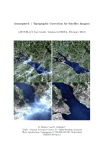
The cover image shows the principal task of an atmospheric processor in the solar reflective spectrum: the input is a digital number (DN) or scaled radiance image with a certain number of
channels, the output is surface reflectance, where the atmospheric influence has been removed.
The input signal consists of path radiance, transmitted radiance from the observed pixel, and radiation from the neighborhood (adjacency effect), schematically represented by the signal components
L1 , L2 , L3 , respectively.
The scaled radiance spectrum shows the influence of the additional path radiance L1 , which has
a strong influence in the blue-green part of the spectrum. In addition, regions with atmospheric
absorption features can be observed. In the output surface reflectance spectrum these atmospheric
features are eliminated.
ATCOR-2/3 Tutorial, Version 1.1, July 2015
Authors:
R. Richter1 and D. Schläpfer2
1 DLR - German Aerospace Center, D - 82234 Wessling , Germany
2 ReSe Applications, Langeggweg 3, CH-9500 Wil SG, Switzerland
c All rights are with the authors of this manual.
R trademark refers to the satellite and airborne versions of the software.
The ATCOR
Distribution:
ReSe Applications Schläpfer
Langeggweg 3, CH-9500 Wil, Switzerland
Updates: see ReSe download page: www.rese.ch/download
Contents
1 Getting Started with ATCOR
1.1 Installation . . . . . . . . . . . . . . . . . . . . . . . . . . . . . . . . . . . . . . . . .
2 Pre-defined sensor
2.1 Input files . . . . . . . . . .
2.2 Read meta file information
2.3 Flat terrain . . . . . . . . .
2.4 Mountainous terrain . . . .
2.5 Output files . . . . . . . . .
2.6 Tiling for very large scenes
6
6
.
.
.
.
.
.
.
.
.
.
.
.
.
.
.
.
.
.
.
.
.
.
.
.
.
.
.
.
.
.
.
.
.
.
.
.
.
.
.
.
.
.
.
.
.
.
.
.
.
.
.
.
.
.
.
.
.
.
.
.
.
.
.
.
.
.
.
.
.
.
.
.
.
.
.
.
.
.
.
.
.
.
.
.
.
.
.
.
.
.
.
.
.
.
.
.
.
.
.
.
.
.
.
.
.
.
.
.
.
.
.
.
.
.
.
.
.
.
.
.
.
.
.
.
.
.
.
.
.
.
.
.
.
.
.
.
.
.
.
.
.
.
.
.
.
.
.
.
.
.
.
.
.
.
.
.
.
.
.
.
.
.
.
.
.
.
.
.
.
.
.
.
.
.
.
.
.
.
.
.
8
8
9
11
16
16
19
3 User-defined sensor
3.1 Preparation phase . . . . . . . .
3.2 Radiometric calibration file . . .
3.3 Spectral smile characterization .
3.4 Post-processing: spectral filtering
3.4.1 Statistical filtering . . . .
3.4.2 Smile interpolation . . . .
.
.
.
.
.
.
.
.
.
.
.
.
.
.
.
.
.
.
.
.
.
.
.
.
.
.
.
.
.
.
.
.
.
.
.
.
.
.
.
.
.
.
.
.
.
.
.
.
.
.
.
.
.
.
.
.
.
.
.
.
.
.
.
.
.
.
.
.
.
.
.
.
.
.
.
.
.
.
.
.
.
.
.
.
.
.
.
.
.
.
.
.
.
.
.
.
.
.
.
.
.
.
.
.
.
.
.
.
.
.
.
.
.
.
.
.
.
.
.
.
.
.
.
.
.
.
.
.
.
.
.
.
.
.
.
.
.
.
.
.
.
.
.
.
.
.
.
.
.
.
.
.
.
.
.
.
.
.
.
.
.
.
.
.
.
.
.
.
.
.
.
.
.
.
20
21
26
26
26
26
28
.
.
.
.
.
.
.
.
.
.
.
.
4 Advanced options
30
4.1 Haze removal . . . . . . . . . . . . . . . . . . . . . . . . . . . . . . . . . . . . . . . . 30
4.2 De-shadowing . . . . . . . . . . . . . . . . . . . . . . . . . . . . . . . . . . . . . . . . 30
4.3 Cast shadow border removal . . . . . . . . . . . . . . . . . . . . . . . . . . . . . . . . 30
5 Miscellaneous
5.1 Default preference parameters
5.2 Cloud and water mask . . . .
5.3 Spectral classification . . . .
5.4 DEM smoothing . . . . . . .
.
.
.
.
.
.
.
.
.
.
.
.
.
.
.
.
.
.
.
.
.
.
.
.
References
.
.
.
.
.
.
.
.
.
.
.
.
.
.
.
.
.
.
.
.
.
.
.
.
.
.
.
.
.
.
.
.
.
.
.
.
.
.
.
.
.
.
.
.
.
.
.
.
.
.
.
.
.
.
.
.
.
.
.
.
.
.
.
.
.
.
.
.
.
.
.
.
.
.
.
.
.
.
.
.
.
.
.
.
.
.
.
.
.
.
.
.
.
.
.
.
.
.
.
.
32
32
32
32
35
36
3
List of Figures
1.1
Top level menu of ATCOR. . . . . . . . . . . . . . . . . . . . . . . . . . . . . . . . .
2.1
2.2
2.3
2.4
2.5
2.6
2.7
2.8
2.9
2.10
2.11
2.12
ATCOR input files. . . . . . . . . .
File selection of buttons. . . . . . .
Sensor meta file selection. . . . . .
Choices in ’Atm. Correction’. . . .
ATCOR2 main menu. . . . . . . .
Spectra module. . . . . . . . . . .
Image processing options. . . . . .
Menu for slope/aspect calculation.
Menu for skyview calculation. . . .
ATCOR3 main menu. . . . . . . .
Panel for DEM files. . . . . . . . .
Panel for tiling of scenes. . . . . .
.
.
.
.
.
.
.
.
.
.
.
.
.
.
.
.
.
.
.
.
.
.
.
.
.
.
.
.
.
.
.
.
.
.
.
.
.
.
.
.
.
.
.
.
.
.
.
.
.
.
.
.
.
.
.
.
.
.
.
.
9
10
11
11
12
14
14
17
17
18
18
19
Steps to define a new user-defined sensor. . . . . . . . . . . . . . . . . . . . . . . .
Sketch of sensor preparation files. . . . . . . . . . . . . . . . . . . . . . . . . . . . .
Definition of sensor parameters. . . . . . . . . . . . . . . . . . . . . . . . . . . . . .
Generation of wavelength / bandwidth file. . . . . . . . . . . . . . . . . . . . . . .
Choices for spectral response functions. . . . . . . . . . . . . . . . . . . . . . . . .
Blackbody temperature for thermal bands. . . . . . . . . . . . . . . . . . . . . . . .
Resampling of atmospheric LUTs. . . . . . . . . . . . . . . . . . . . . . . . . . . .
Post-processing filter modules. . . . . . . . . . . . . . . . . . . . . . . . . . . . . .
Statistical filter menu. . . . . . . . . . . . . . . . . . . . . . . . . . . . . . . . . . .
Example of polishing reflectance spectra of Hyperion data after atmospheric correction incl. smile (top) and using a statistical filter (bottom). . . . . . . . . . . . . .
3.11 Smile interpolation. . . . . . . . . . . . . . . . . . . . . . . . . . . . . . . . . . . . .
.
.
.
.
.
.
.
.
.
20
20
22
22
23
24
25
26
27
3.1
3.2
3.3
3.4
3.5
3.6
3.7
3.8
3.9
3.10
.
.
.
.
.
.
.
.
.
.
.
.
.
.
.
.
.
.
.
.
.
.
.
.
.
.
.
.
.
.
.
.
.
.
.
.
.
.
.
.
.
.
.
.
.
.
.
.
.
.
.
.
.
.
.
.
.
.
.
.
.
.
.
.
.
.
.
.
.
.
.
.
.
.
.
.
.
.
.
.
.
.
.
.
.
.
.
.
.
.
.
.
.
.
.
.
.
.
.
.
.
.
.
.
.
.
.
.
.
.
.
.
.
.
.
.
.
.
.
.
.
.
.
.
.
.
.
.
.
.
.
.
.
.
.
.
.
.
.
.
.
.
.
.
.
.
.
.
.
.
.
.
.
.
.
.
.
.
.
.
.
.
.
.
.
.
.
.
.
.
.
.
.
.
.
.
.
.
.
.
.
.
.
.
.
.
.
.
.
.
.
.
.
.
.
.
.
.
.
.
.
.
.
.
.
.
.
.
.
.
.
.
.
.
.
.
.
.
.
.
.
.
.
.
.
.
.
.
.
.
.
.
.
.
.
.
.
.
.
.
.
.
.
.
.
.
.
.
.
.
.
.
.
.
.
.
.
.
.
.
.
.
.
.
.
.
.
.
.
.
.
.
.
.
.
.
6
. 28
. 29
4.1
Shadow border removal tool . . . . . . . . . . . . . . . . . . . . . . . . . . . . . . . . 31
5.1
5.2
Panel for preference parameters. . . . . . . . . . . . . . . . . . . . . . . . . . . . . . 33
Spectral classification of a Landsat TM subset. . . . . . . . . . . . . . . . . . . . . . 34
4
List of Tables
3.1
Example of a sensor definition file (no thermal bands). . . . . . . . . . . . . . . . . . 21
5
Chapter 1
Getting Started with ATCOR
This tutorial is a quick start guide for the satellite version of ATCOR. It covers the essential information about software installation and licensing as well as the basic steps to perform atmospheric
correction. This tutorial is an addition to the extensive user manual provided with the software.
Please refer to the manual [1]for for details.
1.1
Installation
Please proceed as follows for a new installation of ATCOR:
1. download the software from the ReSE web site ( www.rese.ch/download/ ).
2. unzip the archive and put the created directory to any software installation path.
3. install the license file ’rese license.pro’ provided by email in the atcor 23 directory or any
other valid idl-path location.
4. start IDL and type ’atcor’ on the command line, then the save file ’atcor.sav’ should be
restored and the atcor GUI (graphical user interface) should appear.
Figure 1.1: Top level menu of ATCOR.
Potential problems:
• IDL searches for the license file ’rese license.pro’, make sure such a file does not exist in several
folders.
• IDL searches for the file ’atcor.sav’, make sure only one file exists in all IDL paths (delete or
rename older versions of ’atcor.sav’).
• If licensing fails, ask for debugging instructions at [email protected] .
6
CHAPTER 1. GETTING STARTED WITH ATCOR
7
The next chapter describes the task of atmospheric correction with a pre-defined multispectral
sensor for a flat terrain scene. It is recommended that beginners to ATCOR read this chapter
first before moving to more difficult cases, e.g. scenes with mountainous terrain or hyperspectral
(user-defined) sensors.
Chapter 2
Pre-defined sensor
The input to an atmospheric processor is a grey level or digital number (DN) image for each channel.
The digital number is proportional to the radiance L measured at the sensor:
L = c0 + c1 DN
(2.1)
where c0 , c1 are offset and gain of the radiometric calibration, respectively. Usually, all data
providers deliver scenes with a meta file containing the offset and gain values for each channel. In
addition, the meta file contains information on the solar and viewing geometry, on the geographic
location, etc.
Since different radiance units are used by different data providers, these have to be converted into
the unit employed by ATCOR, namely mW cm−2 sr−1 µm−1 .
ATCOR needs this basic information, then estimates the most important atmospheric parameters
(aerosol and water vapor) to derive the surface reflectance. The schematic sketch on the title page
shows that the total radiance signal L at the sensor consists of three components:
L = L1 + L2 + L3 = c0 + c1 DN
(2.2)
• L1 , path radiance: scattered radiation in the air volume between ground and sensor, consisting
of all photons without ground contact.
• L2 , ground reflectance radiation from a certain pixel.
• L3 , radiation reflected from the neighborhood, scattered once or more times, being propagated
into the direction of the viewed pixel.
After estimating the atmospheric parameters, ATCOR subtracts the radiance components L1 and
L3 from the total at-sensor radiance L, and finally calculates the surface reflectance ρ from the
component L2 with a knowledge of the atmospheric transmittance as well as direct and diffuse solar
flux on the ground. The corresponding atmospheric functions are pre-calculated with a radiative
transfer code (MODTRAN-5) and stored in look-up tables (LUTs) for a large range of weather
conditions and solar/view geometries.
2.1
Input files
The default image file format for ATCOR is the ENVI band sequential (BSQ) format. Other
formats (e.g. BIL = band-interleaved by line, BIP = band-interleaved by pixel, TIFF) should be
8
CHAPTER 2. PRE-DEFINED SENSOR
9
Figure 2.1: ATCOR input files.
converted, e.g. with ATCOR’s File / Export options, see figure 2.2.
After the file format conversion into ENVI band sequential (example file name: ’scene.bsq’), the
next step is the reading of the sensor meta file, which will create the calibration file (’scene.cal’)
and the ATCOR input parameter file (’scene.inn’), see figure 2.1. This completes the preparation
phase and ATCOR can then be started.
It is recommended to start with the simplest case, namely atmospheric correction in flat terrain,
see section 2.3, before moving on to the processing of scenes in mountainous terrain, where a digital
elevation model (DEM) or digital surface model (DSM) is needed, see section 2.4.
Notes of caution:
1. SPOT imagery (SPOT, Kompsat, Formosat, Pleiades) are delivered in the DIMAP format,
and often with the band sequence NIR, Red, Green. Make sure to convert the channels in
the ’scene.bsq’ with ascending wavelength.
2. Landsat-4/5 TM data: ATCOR allows a processing with or without the thermal band 6. If
band 6 is included, it must be layer 6 in the band sequential file ’scene.bsq’, and layer 7 is
the 2.2 µm band.
3. Landsat-7 ETM+ data is delivered with band 6 in the low gain (’band 61’) and high gain
(’and 62’ modes. For consistency with Landsat-4/5 TM only one thermal band can be selected
(either band 61 or band 62) and it must be layer 6 in the band sequential file ’scene.bsq’.
2.2
Read meta file information
The meta file reader provides two input files to ATCOR. When pressing the ’File’ button of the
ATCOR top level menu (see figure 1.1), the choices of figure 2.2 appear.
Select the button ’Read Sensor Meta Data’ and a list of frequently used sensors appears (figure
2.3). The example selects a Worldview-2 metafile (*.IMD). Two input files for ATCOR are created:
• ’*.cal’, containing the radiometric calibration offset and gain per band.
• ’*.inn’, containing the input parameter file for ATCOR. It includes the name of the selected
sensor, and the solar and view geometry for the current scene. Since the atmospheric visibility
(VIS) and ground elevation (h) are not known at this time, they are assigned default values
(VIS=23 km, h=0 km, i.e., sea level). These values can be updated during the ATCOR
processing.
CHAPTER 2. PRE-DEFINED SENSOR
10
Figure 2.2: File selection of buttons.
If the input scene is named ’scene.bsq’, then the ’*.inn’ file only has to be renamed as ’scene.inn’
and all ATCOR input files are supplied.
Note
The meta file reader has no information on the appropriate atmosphere. Therefore, it sets the
following defaults for the .inn file:
• US Standard atmosphere (concerning temperature, pressure, humidity profile). This choice
selects the atmospheric water vapor column and it is not critical for most multispectral
sensors, because their channels are not located in water vapor sensitive spectral regions.
• The elevation is set to zero (sea level). This value might be updated in the ATCOR GUI if
necessary. Height differences up to 300 m have a negligible impact.
• rural aerosol, VIS=23 km. This visibility is only used if no dark reference pixels are found,
see next bullet.
• Parameter npref = 1. This means the visibility is automatically calculated from the scene if
dark reference pixels (dark vegatation, dark soil, water) are found in the scene. This ’variable
visibility’ flag can be disabled, i.e. npref = 0, in the ATCOR GUI by selecting the image
processing option ’Variable Visibility .... No’. Then the specified constant visibility is used.
If the visibility estimator calculates a lower or higher visibility (say VIS=15 km) then the
default VIS=23 km will be overwritten. The meta file reader enables the visibility estimator
flag to provide the necessary flexibility.
Of course, if the scene contains no dark reference pixels, the default visibility VIS=23 km
is used, which might not be correct. However, the user can modify the VIS value (in the
ATCOR GUI) and check its influence in the SPECTRA module, see chapter 2.3.
Unknown meta file
If the reading of a meta file format is not supported for a certain sensor, the user has to generate
the corresponding ’.cal’ file. Attention: when reading the offset, gain values from the meta file take
care of the required ATCOR radiance unit (mW cm−2 sr−1 µm−1 ).
However, the ’.inn’ file is also generated by the ATCOR graphical user interface (GUI), where
widgets are provided for the solar / view geometry. The user has to take this information from the
meta file.
CHAPTER 2. PRE-DEFINED SENSOR
11
Figure 2.3: Sensor meta file selection.
2.3
Flat terrain
The most frequent case is the processing of flat terrain imagery with pre-defined sensors, e.g.
Landsat TM, ETM+, SPOT, Ikonos, Worldview-2 etc. The first prerequisite is the scene data in
the ENVI band-sequential format (’scene.bsq’). In addition, a radiometric calibration file must
exist (’scene.cal’). If the ’Read Sensor Meta Data’ was used, it also generated the input parameter
file (’scene.inn’). Otherwise, this file will be created from the ATCOR GUI, where the user has to
fill out the required widgets.
Figure 2.4 presents the available choices when pressing the button ’Atm. Correction’ of the top
level menu. In this section we describe the option ’pre-defined sensors, flat terrain’. Figure 2.5
shows the corresponding menu.
Figure 2.4: Choices in ’Atm. Correction’.
CHAPTER 2. PRE-DEFINED SENSOR
Figure 2.5: ATCOR2 main menu.
12
CHAPTER 2. PRE-DEFINED SENSOR
13
The ATCOR2 main menu contains the widgets that have a counterpart for the parameters in the
’*.inn’ file. If a widget is changed (e.g. ’Visibility’) and if one of the buttons directly above the
’MESSAGES’ is pressed, then the ’.inn’ file is updated.
The task of the bottom line buttons is
• ’SPECTRA’: calculates the surface reflectance spectrum for a small box in the scene, see
figure 2.6. It allows a coarse check whether the visibility and radiometric calibration yield
reasonable spectra. The example presents a vegetation and soil spectrum in two separate plot
windows. A comparison with some typical library spectra (click button ’reference spectrum’
in the upper right part of the SPECTRA panel) can also be conducted (green spectra in
figure 2.6). More details are given in the User Manual.
• ’AEROSOL TYPE’: proposes the suitable aerosol type (rual, urban, maritime, desert). Requires dark reference pixels in the scene.
• ’VISIBILITY’: estimates the visibility for the currently selected aerosol type. Requires dark
reference pixels in the scene.
• ’INFLIGHT CALIBRATION’: calculates an updated set of calibration coefficients if ground
reflectance spectra are available. See the corresponding chapter in the User Manual.
• ’HELP’: provides a brief help on inflight calibration.
• ’WATER VAPOR’: calculates the water vapor map (without surface reflectance cube) if the
required spectral bands exists. Can be used to test the quality of this map for different
channel combinations without having to compute the reflectance cube.
• ’IMAGE PROCESSING’: starts the image processing in the interactive mode. In case of
very large scenes an error might appear: ’not enough memory to allocate array’. Then start
ATCOR in the ’Tiling’ mode, see last button in figure 2.4.
It is recommended to select an appropiate ’ATMOSPHERIC FILE’ (e.g. mid-latitude summer,
rural aerosol), then press the ’VISIBILITY’ button to obtain the proposed scene visibility. Next,
try the SPECTRA module to check if the proposed visibility yields expected surface reflectance
spectra. Then continue with ’IMAGE PROCESSING’. Here a number of options exist (figure 2.7).
It is recommended to start with the simplest option (everything ’No’) before enabling more elaborate options.
Standard output files after atmospheric correction are:
• A map of pre-classification (’scene hcw.bsq’), containing haze, cloud, water, land, shadow etc.
The generation of this file can be suppressed if the parameter ihcw in the preference settings
is set to zero, see chapter 5.1.
• A map of employed dark reference pixels (’scene atm ddv.bsq’), which is used to calculate
the visibility / aerosol optical thickness. It is not available if the scene is processed with a
constant visibility specification.
• A map of aerosol optical thickness at 550 nm (’scene atm aot.bsq’), not available if the scene
is processed with a constant visibility specification.
• A map of columnar water vapor, if the required spectral bands exist (’scene atm wv.bsq’).
CHAPTER 2. PRE-DEFINED SENSOR
Figure 2.6: Spectra module.
Figure 2.7: Image processing options.
14
CHAPTER 2. PRE-DEFINED SENSOR
• The surface reflectance cube (’scene atm.bsq’).
15
CHAPTER 2. PRE-DEFINED SENSOR
2.4
16
Mountainous terrain
Compared to the flat terrain three additional input files are necessary:
• the digital elevation model (DEM)
• the derived slope map
• the derived aspect map
The first step is to provide a DEM file and to orthorectify the scene with this DEM. The next step
has to compute the mandatory derived files of terrain slope and aspect (unit degrees). This can be
done with the ’Topographic’ functions of ATCOR (or with other software tools):
The following nomenclature is used by ATCOR: the DEM elevation file should have an arbitrary
name (say ’xxx’) followed by ’ ele.bsq’, i.e. ’xxx ele.bsq’. Then the slope and aspect files are
named ’xxx slp.bsq’ and ’xxx asp.bsq’, respectively. The skyview and cast shadow files are optional
because they are only needed for scenes in very steep terrain.
The next two figures show the panels of the slope/aspect and skyview calculations.
Concerning the generation of the ’*.inn’ and ’*.cal’ files from the sensor meta data the reader is
referred to the previous section 2.3.
Now the ’Atm. Correction’ button can be pressed, selecting the option ’ATCOR3: pre-defined
sensors, rugged terrain’. The menu is very similar to the panel in figure 2.5, the only difference is
that the solar azimuth angle is also specified on this graphical interface.
Additionally, another panel appears for the specification of the DEM related files, see figure 2.11.
As a default, the program searches for the DEM files in the same folder as the scene. IF they are
placed elsewhere, press the button ’Update DEM Path’ to specify the appropriate folder. When
processing the scene, the average elevation is extracted from the ’* ele.bsq’ file and put into the
’*.inn’ file. In addition, the file names of the DEM files are automatically included in the *.inn” file.
The action of all other buttons (e.g. ’SPECTRA’, ’VISIBILITY’ etc) is described in the previous
flat terrain section.
2.5
Output files
For a flat terrain processing, the standard output files after atmospheric correction are:
• A map of pre-classification (’scene hcw.bsq’), containing haze, cloud, water, land, shadow etc.
The generation of this file can be suppressed if the parameter ihcw in the preference settings
is set to zero, see chapter 5.1.
CHAPTER 2. PRE-DEFINED SENSOR
Figure 2.8: Menu for slope/aspect calculation.
Figure 2.9: Menu for skyview calculation.
17
CHAPTER 2. PRE-DEFINED SENSOR
Figure 2.10: ATCOR3 main menu.
Figure 2.11: Panel for DEM files.
18
CHAPTER 2. PRE-DEFINED SENSOR
19
Figure 2.12: Panel for tiling of scenes.
• A map of employed dark reference pixels (’scene atm ddv.bsq’), which is used to calculate
the visibility / aerosol optical thickness. It is not available if the scene is processed with a
constant visibility specification.
• A map of aerosol optical thickness at 550 nm (’scene atm aot.bsq’), not available if the scene
is processed with a constant visibility specification.
• A map of columnar water vapor, if the required spectral bands exist (’scene atm wv.bsq’).
• The surface reflectance cube (’scene atm.bsq’).
For a rugged terrain, an additional file is provided containing the illumination map. This is the
cosine of the local solar zenith angle multiplied with a scale factor of 100 and byte coded. The
name is ’scene ilu.bsq’.
2.6
Tiling for very large scenes
For very large scenes a processing may fail with the error message (on the IDL command line)
’Not enough memory to allocate array’.
In this case, the tiling option should be used, see figure 2.4. Figure 2.12 presents the corresponding
menu. The number of tiles (sub-images) in x and y direction can be specified. Then the processing
is performed separately for each tile, and finally all tiles are merged to the original scene size. The
number of tiles should be as small as possible, because the result might depend on the tile definition
(since some steps evaluate statistical properties of tiles which can vary with size). The required
size depends on the memory resources of the machine and the operating system, so it has to be
tested for each machine.
If no output name is specified, the default name is the same as the input file name plus the ’ atm’
appended (i.e. ’tm essen1000 atm.bsq’ in this example).
Chapter 3
User-defined sensor
In principle, the same preparation steps apply as for a pre-defined sensor. Please read chapter 2.
However, some additional steps are needed to define the sensor and to calculate the corresponding
look-up tables for the atmospheric correction. The required additional steps are listed below the
’New Sensor’ entry of the top level ATCOR menu:
Figure 3.1: Steps to define a new user-defined sensor.
Figure 3.2: Sketch of sensor preparation files.
20
CHAPTER 3. USER-DEFINED SENSOR
21
Figure 3.2 presents a sketch of the required preparation files. The part outside the dashed rectangle
is only required for spectrometers affectd by spectral smile. Details are described in the next section.
3.1
Preparation phase
1. Definition of the sensor field-of-view (FOV), number of bands in different spectral regions,
etc. Example: a hyperion sensor with 191 bands shall be created, containing a subset of the
original 242 bands without the very noisy bands. All user-defined sensors are located in the
’../atcor/sensor/’ folder. Therefore, the new ’hyperion191’ sensor description has to be defined
in the folder ’../sensor/hyperion191/’ and the file name must be ’sensor hyperion191.dat’ or
’hyperion191.dat’. The file can be created by copying the ’.dat’ from another sensor and
editing it to update the FOV, number of bands etc.
The file ’sensor hyperion191.dat’ can also be created with a GUI: press the button ’Define
Sensor Parameters’ and fill out the required widgets, see figure 3.3. The next table presents
an example for ’sensor hyperion191.dat’. The last line is only required if the spectral smile
characterization is included, i.e. if the file ’smile poly ord4.dat’ is provided.
0.6
1
0
0
1
0
1
256
191
0
0
5
across-track FOV [degree], pixels per line
first, last reflective band (0.35-2.55 µm)
first, last mid IR band (2.6 -7.1 µm)
first, last thermal band (7.1 -14 µm)
flag for tilt capability (1=yes, 0=no)
required dummy
ismile (0=no, 1=yes), 5 = Gaussian spectral filter function
Table 3.1: Example of a sensor definition file (no thermal bands).
2. Create the wavelength and bandwidth file ’sensor hyperion191.wvl’: press the button ’Create
Wavelength File .wvl from Image Header’. The the menu of figure 3.4 will pop up. Specify the
ENVI image file (already with the subset of 191 bands) and the sensor name ’hyperion191’.
Then an ASCII file with 3 columns is created containing the band number, center wavelength,
and bandwidth for each channel.
3. Create the spectral response files for each band using the ’sensor hyperion191.wvl’, see figure
3.5. Here, different shapes of the channel filter functions can be selected: these correspond
to simple analytical functions, number 5 (Gaussian) is the likely choice for spectrometers.
Then for each channel a normalized spectral response ASCII file with 2 columns (wavelength
in µm, response from 0 to 1) is created, including a header line specifying the number of
spectral points.
These files are later used during the resampling of the high-resolution (’monochromatic’)
spectral database of atmospheric correction functions to obtain sensor-specific LUTs.
If no simple analytic function is able to describe the filter shape, then each channel has to be
defined as tabular data. This information can usually be taken from laboratory measurements.
Again, the response function of each band has to be defined in the same way as for the analytic
functions, i.e., one ASCII file per band with a header line containing the number of spectral
points, then two columns of data (wavelength, spectral response). The files must be named
’band001.rsp’, ’band002.rsp’ etc. In case of less than 100 bands, the numbering is ’band01.rsp’,
CHAPTER 3. USER-DEFINED SENSOR
22
’band02.rsp’, etc. In case of less than 10 bands, the file numbering is ’band1.rsp’, ’band2.rsp’,
etc.
The spectral binning option allows the binning of spectral response functions of the selected
type. This is of interest for sensors with programmable binning of channels, e.g. HySpex. A
binning factor of 2, for example, means that two neighoring bands are combined into a new
band, weighted with their filter functions, and the new sensor has a factor 2 less bands than
the non-binned version.
4. The blackbody functions for each band are only required in case of thermal bands, see figure
3.6. Here the first response file (’band001.rsp’) is selected, and for all thermal bands a
least squares fit of Tbb = f (Lbb ) is performed using the corresponding channel filter files
(’band*.rsp’). Results are written to a ’*.bbfit’ file in the pertaining sensor folder.
5. Sensor-specify atmospheric correction functions (LUTs) have to be calculated from the highresolution spectral database. This is performed by resampling the high-resolution data with
the spectral filter function of each band, see figure 3.7. Different resampling steps are required
for reflective and thermal bands.
Figure 3.3: Definition of sensor parameters.
Figure 3.4: Generation of wavelength / bandwidth file.
CHAPTER 3. USER-DEFINED SENSOR
Figure 3.5: Choices for spectral response functions.
23
CHAPTER 3. USER-DEFINED SENSOR
Figure 3.6: Blackbody temperature for thermal bands.
24
CHAPTER 3. USER-DEFINED SENSOR
Figure 3.7: Resampling of atmospheric LUTs.
25
CHAPTER 3. USER-DEFINED SENSOR
3.2
26
Radiometric calibration file
A radiometric calibration file is needed to convert the scaled image data (digital numbers, DN)
into a physical radiance unit L at the sensor. ATCOR requires the unit mW cm−2 sr−1 µm−1 , i.e.
L = c0 + c1 DN . The corresponding offset and gain values for each band are provided by the
manufacturer. ATCOR requires an ASCII file with 3 columns (wavelength or band number, offset,
gain), and the number of lines corresponds to the number of bands. The recommended extension
of the file name is ’.cal’, e.g. ’hyperion191.cal’. Example: the first spectrometer of Hyperion has
the gain c1=0.0025, the second spectrometer c1=0.00125, and the offset is 0 for all bands.
3.3
Spectral smile characterization
In case of a spectrometer instrument with spectral smile aberrations, the characterization can
be described by a polynomial function. ATCOR uses a 4th-order polynomial for each bannd to
describe the wavelength shift across the detector array. The smile shift is usually measured in the
laboratory. It can also be determined from the image data for certain spectral regions containing
atmospheric absorption features. ATCOR requires the smile description as an ASCII file with 6
columns: The first column contains the channel center wavelength, the remaining columns contain
the 5 coefficients of the 4th-order polynomial, starting with the constant term. For details, read the
corresponding sections in the ATCOR user manual. The file name has to be ’smile poly ord4.dat’,
located in the corresponding sensor folder.
3.4
Post-processing: spectral filtering
In many cases hyperspectral imagery require some post-processing, e.g. a spectral filtering due to
small errors in the spectral band center location, accuracy to the radiative transfer code, interpolation in the LUTs, or assumed extraterrestrial solar irradiance spectrum. Figure 3.8 shows the
post-processing options offered by ATCOR.
Figure 3.8: Post-processing filter modules.
Two options are presented here: the statistical filter and the smile interpolation.
3.4.1
Statistical filtering
Figure 3.9 shows the GUI for polishing hyperspectral data with statistical filters. Four filter types
are offered, but the best choice depends on the sensor performance. Therefore, some trial and error
is necessary to obtain the best results.
The different filters work as follows:
CHAPTER 3. USER-DEFINED SENSOR
27
• Derivative Filter: all spectral bands of the selected window size are taken into account to
calculate derivatives used to reconstruct the value of the center band.
• Neighbor Derivative: the derivatives of all bands except the center band are used to reconstruct the value of the center band.
• Lowpass Filter: only smoothing is performed, no derivatives are calculated.
• Savitzky-Golay: a 4th-order polynomial fit is performed for the total window size. Note: this
filter does not account for the wavelength-spacing of bands, i.e. it assumes equidistant bands.
The input file is usually the reflectance product after atmospheric correction. For the spectral
response the first channel is selected (’band001.rsp’). The default number of polishing bands on
each side of the center band is 3, i.e., the total number is 7 (3 on each side plus the center band).
The smoothing factor is defined as:
1. slight smoothing, weighting of bands (left/center/right) = (1/4/1)
2. moderate smoothing, weighting of bands (left/center/right) = (1/2/1)
3. standard smoothing, weighting of bands (left/center/right) = (1/1/1)
4. and higher: same as standard smoothing.
More details are described in reference [3].
Figure 3.9: Statistical filter menu.
Figure 3.10 presents examples of polishing reflecance spectra using a statistical filter, see [3].
CHAPTER 3. USER-DEFINED SENSOR
28
Figure 3.10: Example of polishing reflectance spectra of Hyperion data after atmospheric correction incl.
smile (top) and using a statistical filter (bottom).
3.4.2
Smile interpolation
Figure 3.11 presents the GUI for a smile interpolation. Three options for resampling are offered as
described in this GUI. The selected option indicates: the spectral surface reflectance cube (after
atmospheric correction) is resampled to a new reference wavelength grid using the wavelength
average over all detector columns (per band).
CHAPTER 3. USER-DEFINED SENSOR
Figure 3.11: Smile interpolation.
29
Chapter 4
Advanced options
Some of the advanced options are briefly described here or a reference is given to the User Manual.
The reasons for the reference are twofold: this tutorial is intended to present only the basic options,
and the User Manual already covers the more complex subjects. On the other hand, a quick
reference is useful where the material can be found.
4.1
Haze removal
This topic is covered extensively in the User Manual [1].
4.2
De-shadowing
This topic is also discussed in detail in the User Manual [1], chapter 10. Two de-shadowing
algorithms are available: the matched filter approach and the illumination based approach. The
last method requires a DEM and the subsequent calculation of the illumination map. However,
as a special case, a float illumination map can also be generated based on scene-derived spectral
indices, with or without the topography files. The image scene derived illumination map is stored
as the first band of a multi-layer file, coded in float. Use the ’Topographic’, ’Image Based Shadows’
module of the ATCOR main panel to create such a file. If the scene is named ’scene.bsq’, then
the corresponding illuminatiion file is named ’scene ilu.bsq’. And if the de-shadowing option is
specified, then the de-shadowing with this file has the first priority. If the matched filter method
is selected, then the ’scene ilu.bsq’ has to be (temporarily) renamed, e.g. as ’scene iluq.bsq’ or it
has to be moved to a different folder.
4.3
Cast shadow border removal
This routine can be used after cast shadow correction in case the borders of the shadows show
dark or bright artifacts. It corrects the imagery by adjusting the brightness to the direct neighbor
pixels. Using the illumination file, all pixels at the cast shadow borders are first identified and a
buffer along the borders is calculated using the border width. Secondly, a brightness correction
factor is calculated for each pixel in the border lines using the relative brightness in comparison to
its neighbors. The pixels are then corrected using this relative difference in a multiplicative way.
Input File A hyperspectral image cube, usually the output of atmospheric correction ∗ atm.bsq
30
CHAPTER 4. ADVANCED OPTIONS
31
Illumination/Cast Shadow File illumination file containing a shadow mask which had been
applied to the image during atmospheric correction.
Options Two options for alternate processing are available (try those in case the artifacts are not
well removed):
Adjust spectral mean: An average additional correction factor is applied to the border pixels
in order to correct for spectral variation of the brightness difference.
Interpolate Borders: The border pixels are interpolated from their neighbours, overwriting
the original values.
Shadow Border Width: the with of the border to be corrected/interpolated..
Output:
A cube containing the filtered image data is generated and the ENVI header is copied to the new
file.
Figure 4.1: Shadow border removal tool
Chapter 5
Miscellaneous
5.1
Default preference parameters
In addition to the processing parameters of the ”.inn” file there are a number of default settings
(e.g. thresholds for cloud and water masking, definition of atmospheric absorption regions etc)
which usually are kept constant. However, if necessary they might be edited (activate button ’Edit
Preferences’, see figure 2.2.) A detailed description of these parameters is given in the User Manual.
Figure 5.1 shows the user interface for the preference parameters.
5.2
Cloud and water mask
The cloud mask for an input file ”scene.bsq” is included in the file ”scene hcw.bsq”, which also
contains the haze (if the haze option is set) and water pixels. The calculation is solely based on a
spectral threshold criterion with the default reflectance threshold T=25% in the blue/green band.
All pixels with reflectance higher than this threshold are labeled ’cloud’. Bright soils, sand, or roofs
might exceed this threshold. Therefore, a more realistic cloud mask may need an adjustment of
this threshold (in the preference parameter file, see figure 5.1, depending on scene content.
A better cloud threshold usually also improves the haze removal (if set).
The water mask is also included in the file ”scene hcw.bsq”. Again, it is exclusively calculated with
spectral criteria set in the preference parameter file. Depending on the available spectral bands
and the turbidity of water bodies in the scene, these default thresholds might have to be modified.
5.3
Spectral classification
After atmospheric correction the surface reflectance image (”scene atm.bsq”) can be fed into a fully
automatic spectral classifier (top level menu ’Tools’, then ’SPECL: Spectral Reflectance Classifier’).
The output file (”scene atm cla.bsq”) contains a number of fixed spectral classes (e.g. bright and
dark vegetation, soil, water) which might be useful as a first orientation. However, these are not
land use classes. An example is given in figure 5.2.
32
CHAPTER 5. MISCELLANEOUS
Figure 5.1: Panel for preference parameters.
33
CHAPTER 5. MISCELLANEOUS
Figure 5.2: Spectral classification of a Landsat TM subset.
34
CHAPTER 5. MISCELLANEOUS
5.4
35
DEM smoothing
Spatial artifacts often occur in case of processing mountainous terrain data, especially for high
spatial resolution imagery. These artifacts are clearly visible in the slope and illumination maps,
and therefore also in the output surface reflectance product. There are several options to improve
the situation:
• smooth the digital elevation model and the derived products (slope, aspect) using the function
DEM Smoothing of the ’Topographic’ top level menu. The default kernel size is 3 (pixels),
but larger kernels might be necessary depending on the spatial resolution of the image. This
will reduce the high spatial frequency content.
• Better results can sometimes be obtained by using a larger kernel size for the slope / aspect
maps than for the elvation.
• The slope / aspect maps often achieve a better quality if they are expanded, then smoothed,
then shrinked to the original size. Then the following steps may be tried to improve the
results:
- FLOAT (elevation file) if integer coded
- Calculate slope and aspect with a low pass filter of 5x5 pixels
- Resize slope / aspect file: factor 4 larger
- Apply a low pass filter (7x7 pixels)
- Resize with factor 0.25 using nearest neigbor to obtain the original size.
• Switch off the cast shadow correction (by leaving the field empty where the cast shadow map
is defined in the DEM panel).
• Use the empirical BRDF correction for rugged terrain.
Bibliography
[1] Richter, R. and D. Schläpfer, ”Atmospheric / topographic correction for satellite imagery:
ATCOR-2/3 User Guide”, DLR IB 565-01/13, Wessling, Germany (2013).
[2] Richter, R., and D. Schläpfer, ”Atmospheric / topographic correction for airborne imagery:
ATCOR-4 User Guide”, DLR IB 565-02/13, Wessling, Germany (2013).
[3] , D. Schläpfer, and R. Richter, ”Spectral polishing filters of high resolution imaging spectroscopy data”, Imaging Spectroscopy (2011).
36