Download Neuralnets for Multivariate And Time Series Analysis

Neuralnets for Multivariate And Time Series Analysis
(NeuMATSA): A User Manual
(Version 3.1)
MATLAB codes for:
Nonlinear principal component analysis
Nonlinear canonical correlation analysis
Nonlinear singular spectrum analysis
William W. Hsieh
Department of Earth and Ocean Sciences,
University of British Columbia,
Vancouver, B.C. V6T 1Z4, Canada
c 2005
Copyright William W. Hsieh
1
1
1
INTRODUCTION
2
Introduction
For a set of variables {xi }, principal component analysis (PCA) (also called Empirical Orthogonal
Function analysis) extracts the eigenmodes of the data covariance matrix. It is used to (i) reduce
the dimensionality of the dataset, and (ii) extract features from the dataset. When there are
two sets of variables {xi } and {yj }, canonical correlation analysis (CCA) finds the modes of
maximum correlation between {xi } and {yj }, rendering CCA a standard tool for discovering
relations between two fields. The PCA method has also been extended to become a multivariate
spectral method— the singular spectrum analysis (SSA). See von Storch and Zwiers (1999) for a
description of these classical methods.
Neural network (NN) models have been widely used for nonlinear regression and classification
(with codes available in many computer packages, e.g. in the MATLAB Neural Network toolbox).
Recent developments in neural network modelling have further led to the nonlinear generalization
of PCA, CCA and SSA.
This manual for NeuMATSA (Neuralnets for Multivariate And Time Series Analysis) describes
the neural network codes developed at UBC for nonlinear PCA (NLPCA), nonlinear CCA (NLCCA), and nonlinear SSA (NLSSA). There are several approaches to nonlinear PCA; here, we
follow the Kramer (1991) approach, and the Kirby and Miranda (1996) generalization to closed
curves. Options of regularization with weight penalty have been added to these models. The
NLCCA model is based on that proposed by Hsieh (2000).
To keep this manual brief, the user is referred to the review paper Hsieh (2004) for details.
This and other relevant papers are downloadable from the web site:
http://www.ocgy.ubc.ca/projects/clim.pred/download.html.
This manual assumes the reader is already familiar with Hsieh (2004), and is aware of the relatively
unstable nature of neural network models because of local minima in the cost function, and the
danger of overfitting (i.e. using the great flexibility of NN models to fit to the noise in the data).
The codes are written in MATLAB using its Optimization Toolbox, and should be compatible
with MATLAB 7, 6.5, and 6.
This manual is organized as follows: Section 2 describes the NLPCA code of Hsieh (2001a),
which is based on Kramer (1991). Section 3 describes the ‘NLPCA.cir’ code, i.e. the NLPCA
generalized to closed curves by having a circular neuron at the bottleneck, as in Hsieh (2001a),
which follows Kirby and Miranda (1996). This code is also used for NLSSA (Hsieh and Wu,
2002). Section 4 describes the NLCCA code of Hsieh (2001b), which is an improved version of
Hsieh (2000). A demo problem is set up in each section. The sans serif font is used to denote
the names of computer commands, files and variables. Section 5 is on hints and trouble-shooting.
The latest version of codes is based on Hsieh (2004).
Whether the nonlinear approach has a significant advantage over the linear approach is highly
dependent on the dataset— the nonlinear approach is generally ineffective if the data record is
short and noisy, or the underlying relation is essentially linear. Because of local minima in the
cost function, an ensemble of optimization runs from random initial weight parameters is needed,
and the best member of the ensemble selected as the solution. There is no guarantee that the
best member is close to the global minimum. Presently, the number of hidden neurons and the
weight penalty parameters are determined largely by a trial and error approach. Future research
will hopefully provide more guidance on their choice.
The computer programs are free software under the terms of the GNU General Public License
as published by the Free Software Foundation. Please read the file ‘LICENSE’ in the program
directory before using the software.
2
NLPCA
2
2.1
3
Nonlinear Principal Component Analysis
Files in the directory for NLPCA
The downloaded tar file NLPCA.tar can be uncompressed with the Unix tar command:
tar -xf NLPCA.tar
and a new directory NLPCA will be created containing the following files:
setdat.m sets up the demo problem, produces a demo dataset xdata which is stored in the file
data1.mat. This demo problem is instructive on how NLPCA works. To see the demo
dataset, the reader should get onto MATLAB, and type in: setdat
which also creates a postscript plot file tempx.ps. The plot displays the two theoretical modes,
and the data xdata (generated from the two theoretical modes plus a little Gaussian noise)
(shown as dots). The objective is to use NLPCA to retrieve the two underlying theoretical
modes from xdata.
nlpca1.m is the main program for calculating the NLPCA mode 1. (Here xdata is loaded). To
run NLPCA on the demo dataset on unix, use:
matlab < nlpca1.m > out1new &
(The ‘&’ allows unix to run the job on the background, as this run could take a good fraction
of an hour). Compare the new output file out1new with the downloaded output file out1 in
this directory; they should be similar. The user should then use nlpca1.m as a template for
his/her own main program.
plmode1.m plots the output mode 1, also writing out the plot on an (encapsuled) postscript file.
Alternatively, pltmode1.m gives a more compact plot.
nlpca2.m is the main program for calculating the NLPCA mode 2, after removing the NLPCA
mode 1 from the data. On unix, use: matlab < nlpca2.m > out2new &
Compare the new output file out2new with out2.
plmode2.m plots the output mode 2, and writes out the plot on a postscript file. Alternatively,
pltmode2.m gives a more compact plot.
param.m contains the parameters for the problem. It contains the parameters for the demo
problem. After the demo, the user will need to put the parameters relevant to his/her
problem into this file.
out1 and out2 are the downloaded output files from the UBC runs of nlpca1.m and nlpca2.m for
the demo problem. Compare them with the new output files out1new and out2new generated
by the user.
mode1 m1.mat, ..., mode1 m4.mat are the extracted nonlinear mode 1, with m (the number of
hidden neurons in the encoding layer) = 1, 2, 3, 4, respectively. (These files were downloaded
originally, but if you have rerun the demo problem, nlpca1.m would overwrite these files).
After removing NLPCA mode 1 (with m = 2) from the data, the residual was put into the
NLPCA model again to extract the second NLPCA mode, again with m varying from 1 to
4, yielding the files mode2 m1.mat,... mode2 m4.mat, respectively.
linmode1.mat is the extracted linear mode 1 (i.e. the PCA mode 1).
2
NLPCA
4
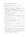
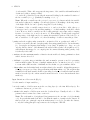
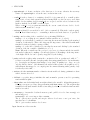
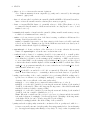
Figure 1: The NN model for calculating nonlinear PCA (NLPCA). There are 3 ‘hidden’ layers of
variables or ‘neurons’ (denoted by circles) sandwiched between the input layer x on the left and
the output layer x on the right. (In the code, xdata is the input, while xi is the output). Next
to the input layer is the encoding layer, followed by the bottleneck layer (with a single neuron
u), which is then followed by the decoding layer. A nonlinear function maps from the higher
dimension input space to the lower dimension bottleneck space, followed by an inverse transform
mapping from the bottleneck space back to the original space represented by the outputs, which
are to be as close to the inputs as possible by minimizing the cost function J = x − x 2 . Data
compression is achieved by the bottleneck, with the bottleneck neuron giving u, the nonlinear
principal component. In the current version, more than 1 neuron is allowed in the bottleneck
layer.
manual.m contains the online manual. To see manual while in MATLAB, type in: help manual
———
The remaining files do not in general require modifications by the user:
chooseTestSet.m randomly divides the dataset into a training set and a test set (also called a
validation set). Different ensemble members will in general have different training datasets
and different test sets.
calcmode.m computes the NLPCA mode (or PCA mode).
costfn.m computes the cost function.
mapu.m maps from xdata to u, the nonlinear PC (i.e. the value of the bottleneck neuron) (Fig.
1).
invmapx.m computes the inverse map from u to xi, where xi is the NLPCA approximation to the
original xdata.
nondimen.m and dimen.m are used for scaling and descaling the data. The input are nondimensionalized according to the scaling option selected, NLPCA is then performed, and the final
results are again dimensionalized.
———
extracalc.m (optional) can be used for projecting new data onto an NLPCA mode, or for examining the solution of any ensemble member from a saved NLPCA run.
2
NLPCA
2.2
5
Parameters stored in param.m for NLPCA
Parameters are classified into 3 categories, ‘*’ means the user normally has to change the value to
fit the problem. ‘+’ means the user may want to change the value, and ‘−’ means the user rarely
has to change the value.
+ iprint = 0, 1, or 2 increases the amount of printout.
Note: Printout summary from an output file (e.g. out1) can be extracted by the unix grep
command: grep # out1
− isave= 1 only saves the best solution in a .mat file, plus W (containing all weight and bias
parameters) and MSEx (mean square error) of all ensemble members. isave = 2 saves all
ensemble member solutions (more memory required).
− linear = 0 means NLPCA; linear = 1 essentially reduces to PCA. [When linear = 1, it is
recommended that m, the number of hidden neurons in the encoding layer, be set to 1, and
testfrac (see below) be set to 0].
* nensemble is the number of members in the ensemble. (Many ensemble members may converge
to shallow local minina and hence wasted).
− testfrac = 0 does not reserve a portion of the data for testing or validation. All data are used
for training. Best if data is rather clean, or a linear solution is wanted.
testfrac > 0 (usually between 0.1 to 0.2), then a fraction of the data record will be randomly
selected as test data. Training is stopped if the MSE increases in the test data by more
than the relative threshold given by earlystop tol.
Note: with testfrac > 0, different ensemble members will work with different training
datasets, so there will be more scatter in the solutions of individual ensemble members
than when testfrac = 0 (where all members have the same training dataset, as all data are
used for training).
+ segmentlength = 1 if autocorrelation of the data is not of concern; otherwise the user might
want to set segmentlength to about the autocorrelation time scale. Data for training and
testing are chosen in segments with length equal to segmentlength.
− overfit tol is the tolerance for overfitting, should be 0 (recommended) or a small positive
number (0.1 or less). Only ensemble members having MSE over the test set no worse than
(MSE over the training set)*(1+overfit tol) are accepted, and the selected solution is the
member with the lowest MSE over all the data.
When overfit tol = 0, program automatically chooses an overfit tolerence level to decide
which ensemble members to accept. [The program calculates overfit tol2, the average value
of MSExtest − MSExtrain for ensemble members where MSExtest is less than MSExtrain, i.e.
MSE for the test data is less than that for the training data. The program then also accepts
ensemble members where MSExtest exceeds MSExtrain by no more than overfit tol2].
− earlystop tol should be around 0.05 to 0.15. (0.1 recommended). This is the ‘early stopping’
method. Best if data is noisy, i.e. overtraining to fit the noise in the data is to be prevented.
* xscaling controls scaling of the x variables before performing NLPCA.
= −1, no scaling (not recommended unless variables are of order 1).
= 0, scales all the xi variables by removing the mean and dividing by the standard deviation
2
NLPCA
6
of each variable. [This could exaggerate the importance of the variables with small standard
deviations, leading to strange results].
= 1, scales all xi variables by removing the mean and dividing by the standard deviation of
the 1st x variable (i.e. x1 ). (Similarly for xscaling = 2, 3, ...)
Note: When the x variables are the principal components of a dataset and the 1st variable
is from the leading mode, xscaling = 1 is strongly preferred. [If xscaling = 0, the importance
of the higher PC modes can be greatly exaggerated by the scaling].
For instance, if the x1 variable ranges from 0 to 3, and x2 from 950 to 1050, then poor
convergence can be expected from setting xscaling = −1, while xscaling = 0 should do much
better. However, if the xi variables are the leading principal components, with x1 ranging
from 0 to 9, x2 from -1 to 2, and x3 from 0 to 1.5, then xscaling = 0 will greatly exaggerate
the importance of the higher modes by causing the standard deviations of the scaled x1 , x2
and x3 variables to be all equal to one, whereas xscaling = 1 will not cause this problem.
* penalty scales the weight penalty term in the cost function. If 0, no penalty used, while 1e−6 0.1 uses a reasonable amount of weight penalty. Increasing penalty leads to less nonlinearity
(i.e. less wiggles and zigzags when fitting to noisy data). If penalty is too large, one gets
only the linear solution— and ultimately the trivial solution (where all weights are zero),
with all input data mapped to one output point. Recommend starting with a penalty of say
0.1, then try 0.01, 0.001, . . .
+ maxiter scales the maximum number of function iterations allowed during optimization. Start
with 1, increase if needed.
+ initRand = a positive integer, initializes the random number generator, used for generating
random initial weights. Because of multiple minima in the cost function, it is a good idea
to rerun with a different value of initRand, and check that one gets a similar solution.
− initwt radius controls the initial random weight radius for the ensemble. Adjust this parameter
if having convergence problem. (Suggest starting with initwt radius = 1). The weight radius
is smallest for the first ensemble member, increasing by a factor of 4 when the final ensemble
member is reached (so the earliest ensemble members tend to be more linear than the later
members).
Input dimensions of the network (Fig. 1):
* l is the number of input variables xi .
* m is the number of hidden neurons in the encoding layer (i.e. the first hidden layer). For
nonlinear solutions, m ≥ 2 is needed.
− nbottle is the number of hidden neurons in the bottleneck layer. Usually, nbottle = 1. This
parameter has been introduced since version 3.1.
Note: The total number of (weight and bias) parameters is 2l × m + 4m + l + 1 (for nbottle
= 1). In general this number should be less than the number of samples in the dataset. If
this is not the case, principal component analysis may be needed to pre-filter the dataset,
so only the leading principal components are used as input to NLPCA.
2
NLPCA
2.3
7
Variables in the codes for NLPCA
The reader can skip this subsection if he/she does not intend to modify the basic code.
Global variables are given by:
global iprint isave linear nensemble testfrac segmentlength ...
overfit tol earlystop tol xscaling penalty maxiter initRand ...
initwt radius options n l m nbottle iter Jscale xmean xstd...
ntrain xtrain utrain xitrain ntest xtest utest xitest MSEx ...
ens accept ens MSEx ens W ens utrain ens xitrain ens utest ens xitest
If you add or remove variables from this global list, it is CRITICAL that the same changes
are made on ALL of the following files:
nlpca1.m, nlpca2.m, param.m, calcmode.m, costfn.m, mapu.m, invmapx.m, extracalc.m.
options are the options used for the m-file fminu.m in the MATLAB optimization toolbox.
n is the number of samples [automatically determined from xdata].
xdata is an l × n data matrix, as there are l ‘xi ’ variables (i = 1, . . . , l), and n samples or time
measurements.
(A common error is to input an n × l data matrix, i.e. the transpose of the correct matrix,
which leads MATLAB to complain about incorrect matrix dimensions).
If xdata contains time series data, it is useful to record the measurement time in the variable
tx (a 1 × n vector). The variable tx is not used by NLPCA in the calculations.
nbottle is the number of bottleneck neurons.
iter is the number of function iterations.
Jscale is a scale factor for the cost function J.
xmean and xstd are the means and standard deviations of the xdata variables.
ntrain, ntest are the number of samples for training and for testing.
xtrain, xtest are the portions of xdata used for training and testing.
utrain, utest are the bottleneck neuron values (the NLPC) during training and testing. [mean(utrain)
= 0 and utrain*utrain /ntrain = 1 are forced on the cost function J.]
xitrain, xitest are the model predicted values for x during training and testing.
MSEx is the mean squared error over all data (training+testing).
ens accept has value 1 if the ensemble member passed the overfit test, otherwise 0.
ens MSEx saves the MSEx, and ens W the weights W for all ensemble members.
When isave = 2, all the ensemble solutions, i.e. ens utrain ens xitrain ens utest ens xitest are saved.
(This could increase memory usage considerably).
3
NLPCA.CIR
3
3.1
8
Nonlinear Principal Component Analysis with a circular bottleneck neuron
Files in the directory for NLPCA.cir
The downloaded tar file NLPCA.cir.tar can be uncompressed with the Unix tar command:
tar -xf NLPCA.cir.tar
and a new directory NLPCA.cir will be created containing the following files:
setdat.m sets up the demo problem, produces a demo dataset xdata which is stored in the file
data1.mat, and creates a postscript plot file tempx.ps. The plot shows the two theoretical
modes, and the input data as dots. The user should go through the demo as in Sec.2.
nlpca1.m is the main program for calculating the NLPCA.cir mode 1. The user should later use
nlpca1.m as a template for his/her own main program.
nlpca2.m is the main program for calculating the NLPCA.cir mode 2.
param.m contains the parameters for the problem. The user will need to put the parameters
relevant to his/her problem into this file.
out1 and out2 are the output files from running nlpca1.m and nlpca2.m respectively.
mode1 m1.mat, ..., mode1 m4.mat are the extracted nonlinear mode 1 with m (the number of
hidden neurons in the encoding layer) = 1, 2, 3, 4, respectively.
After removing mode 1 (with m = 2) from the data, the residual is input into the NLPCA.cir
model again to extract the second mode, again with m varying from 1 to 4, yielding the files
mode2 m1.mat,..., mode2 m4.mat, respectively.
linmode1.mat is the extracted linear mode 1.
plmode1.m plots the output mode 1, also writing out the plot on an (encapsuled) postscript file.
Alternatively, pltmode1.m gives a more compact plot.
plmode2.m plots the output mode 2. Alternatively, pltmode2.m gives a more compact plot.
plotpq.m plots the data projected onto the p-q space for modes 1 and 2, and produces a postscript
plot file temppq.ps.
manual.m contains the online manual.
———
The following files do not in general require modifications by the user:
chooseTestSet.m divides the dataset into a training set and a test set.
calcmode.m computes the NLPCA.cir mode.
costfn.m computes the cost function.
mappq.m maps from the input neurons xdata to the bottleneck (p, q) (Fig. 2).
invmapx.m computes the inverse map from (p, q) to the output neurons xi, where xi is the NLPCA
approximation to the original xdata.
3
NLPCA.CIR
9
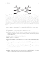
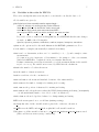
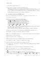
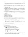
Figure 2: The NLPCA with a ‘circular neuron’ at the bottleneck. Instead of having one bottleneck
neuron u as in Fig.1, there are now two neurons p and q constrained to lie on a unit circle in
the p-q plane, so there is only one free angular parameter (θ). This is also the network used
for performing NLSSA (Hsieh and Wu, 2002), where the inputs to this network are the leading
principal components from the singular spectrum analysis of a dataset.
nondimen.m and dimen.m are used for scaling and descaling the data.
———
extracalc.m (optional) can be used for projecting new data onto an NLPCA.cir mode, or for
examining the solution of any ensemble member from a saved NLPCA.cir run.
3.2
Parameters stored in param.m for NLPCA.cir
Parameters are classified into 3 categories, ‘*’ means user normally has to change the value to
fit the problem. ‘+’ means user may want to change the value, and ‘−’ means user rarely
has to change the value.
+ iprint = 0, 1, or 2 increases the amount of printout.
− isave = 1 only saves the best solution in a .mat file, plus W (containing all weight and bias
parameters) and MSEx (mean square error) of all ensemble members.
isave= 2 saves all ensemble member solutions (more memory required).
− linear = 0 means NLPCA.cir. [linear = 1 uses linear transfer functions, which are not meaningful with a circular neuron, hence not a true option].
* nensemble is the number of members in the ensemble. (Many ensemble members may converge
to shallow local minina and hence wasted).
− testfrac = 0 does not reserve a portion of the data for testing or validation. All data used for
training. Best if data is rather clean.
testfrac > 0 (usually between 0.1 to 0.2), then a fraction of the data record will be randomly
selected as test data. Training is stopped if the MSE (mean squared error) increases in the
test data by more than the relative threshold given by earlystop tol.
3
NLPCA.CIR
10
+ segmentlength = 1 if autocorrelation of the data is not of concern; otherwise the user may
want to set segmentlength to about the autocorrelation time scale.
− overfit tol is the tolerance for overfitting, should be 0 (recommended) or a small positive
number (0.1 or less). Only ensemble members having MSE over the test set no worse than
(MSE over the training set)*(1+overfit tol) are accepted, and the selected solution is the
member with the lowest MSE over all the data.
When overfit tol = 0, program automatically chooses an overfit tolerence level to decide
which ensemble members to accept.
− earlystop tol should be around 0.05 to 0.15. (0.1 recommended). This is the ‘early stopping’
method. Best if data is noisy, i.e. overtraining to fit the noise in the data is to be prevented.
* xscaling controls scaling of the x variables before performing NLPCA.cir.
xscaling = −1, no scaling (not recommended unless variables are of order 1).
xscaling = 0, scales all the xi variables by removing the mean and dividing by the standard
deviation of each variable. [This could exaggerate the importance of the variables with small
standard deviations, leading to strange results].
xscaling = 1, scales all xi variables by removing the mean and dividing by the standard
deviation of the 1st x variable. (Similarly for 2, 3, ...)
Note: When the x variables are the principal components of a dataset and the 1st variable
is from the leading mode, xscaling = 1 is strongly preferred. [If xscaling = 0, the importance
of the higher PC modes can be greatly exaggerated by the scaling].
* penalty scales the weight penalty term in the cost function. If 0, no penalty used, while 1e−6 0.1 uses a reasonable amount of weight penalty. Increasing penalty leads to less nonlinearity
(i.e. less wiggles and zigzags when fitting to noisy data). If penalty is too large, one gets
only the linear solution— and ultimately the trivial solution (where all weights are zero),
with all input data mapped to one output point. Recommend starting with a penalty of say
0.1, then try 0.01, 0.001, . . .
+ maxiter scales the maximum number of function iterations allowed during optimization. Start
with 1, increase if needed.
+ initRand = a positive integer, initializes the random number generator, used for generating
random initial weights.
− initwt radius controls the initial random weight radius for the ensemble. Adjust this parameter
if having convergence problem. (Suggest starting with initwt radius = 1). The weight radius
is smallest for the first ensemble member, increasing by a factor of 4 when the final ensemble
member is reached.
+ zeromeanpq = 1 means the bottleneck neurons p and q will be forced to have mean(p) ≈ 0
and mean(q) ≈ 0.
zeromeanpq = 0 does not impose this constraint.
The ‘0’ option is more general, and can give either a closed curve or an ‘open’ curve, but
may have more local minima.
The ‘1’ option tends towards a closed curve.
Input dimensions of the networks:
3
NLPCA.CIR
11
* l is the number of input variables xi .
* m is the number of hidden neurons in the first hidden layer.
Note: The total number of free (weight and bias) parameters is 2l × m + 6m + l + 2. In
general this number should be less than the number of samples in the dataset. If this is not
the case, principal component analysis may be needed to pre-filter the dataset, so only the
leading principal components are used as input to NLPCA.cir.
3.3
Variables in the codes for NLPCA.cir
The reader can skip this subsection if he/she does not intend to modify the basic code.
Global variables are given by:
global iprint isave linear nensemble testfrac segmentlength ...
overfit tol earlystop tol xscaling penalty maxiter initRand ...
initwt radius options zeromeanpq n l m iter Jscale xmean xstd...
ntrain xtrain ptrain qtrain xitrain ntest xtest ptest qtest...
xitest MSEx ens accept ens MSEx ens W ens ptrain ens qtrain...
ens xitrain ens ptest ens qtest ens xitest
If you add or remove variables from this global list, it is CRITICAL that the same changes
are made on ALL of the following files:
nlpca1.m, nlpca2.m, param.m, calcmode.m, costfn.m, mappq.m, invmapx.m, extracalc.m.
options are the options used for the m-file fminu.m in the MATLAB optimization toolbox.
n is the number of samples [automatically determined from xdata].
xdata is an l × n data matrix, as there are l ‘xi ’ variables, and n samples or time measurements.
iter is the number of function iterations.
Jscale is a scale factor for the cost function J.
xmean and xstd are the means and standard deviations of the xdata variables.
ntrain, ntest are the number of samples for training and for testing.
xtrain, xtest are the portions of xdata used for training and testing.
ptrain, ptest are the bottleneck neuron values (the NLPC) during training and testing. Similarly
for qtrain, qtest.
xitrain, xitest are the model predicted values for x during training and testing.
MSEx is the mean squared error of x over all data (training+testing).
ens accept has value 1 if the ensemble member passed the overfit test, otherwise 0.
ens MSEx saves the MSEx, and ens W the weights W for all ensemble members.
When isave = 2, all the ensemble solutions, i.e. ens utrain ens xitrain ens utest ens xitest are
saved. (This could increase memory usage considerably).
4
NLCCA
4
12
Nonlinear Canonical Correlation Analysis
The downloaded tar file NLCCA.tar can be uncompressed with the Unix tar command:
tar -xf NLCCA.tar
and a new directory NLCCA will be created containing the following files:
4.1
Files in the directory for NLCCA
set2dat.m sets up the demo problem, produces two datasets xdata and ydata which are stored
in the file data1.mat. It also produces two postscript plot files tempx.ps and tempy.ps, with
tempx.ps containing the xdata (shown as dots), and its two underlying theoretical modes,
and tempy.ps containing the ydata and its two theoretical modes. The objective is to use
NLCCA to retrieve the two underlying theoretical modes from xdata and ydata.
nlcca1.m is the main program for calculating the NLCCA mode 1. (Here the datasets xdata and
ydata are loaded). The user should use this file as a template for his/her own main program.
nlcca2.m is the main program for calculating the NLCCA mode 2.
param.m contains the parameters for the problem. The user will need to put the parameters
relevant to his/her problem into this file.
out1 and out2 are the outputs from running nlcca1 and nlcca2 respectively.
mode1 h2.mat and mode1 h3.mat are the extracted nonlinear mode 1 with number of hidden
neurons l2 = m2 = 2 and 3, respectively. After subtracting mode1 (with l2 = m2 = 3) from
the data, the residual was fed into the NLCCA model to extract the second NLCCA mode—
again with the number of hidden neurons l2 = m2 = 2, 3, yielding the files mode2 h2.mat
and mode2 h3.mat, respectively.
linmode1 h1.mat and linmode2 h1.mat are the extracted linear modes 1 and 2.
plmode1.m plots the output mode 1, producing two postscript plot files, whereas pltmode1.m
produces more compact plots onto one postscript file.
plmode2.m plots the output mode 2, producing two postscript plot files, whereas pltmode2.m
produces more compact plots onto one postscript file.
manual.m contains the online manual.
———
The following files do not in general require modifications by the user:
chooseTestSet.m divides the dataset (xdata and ydata) into a training set and a test set.
chooseTestuv.m divides the nonlinear canonical variates u and v (Fig. 3) into a training set and
a test set.
calcmode.m computes the NLCCA mode (or CCA mode). NLCCA uses 3 neural networks (Fig.
3) with 3 cost functions J, J1 and J2, and weight vectors W, W1 and W2, respectively. The
best ensemble member is selected for the forward map (x, y) → (u, v), and its (u, v) become
the input to the two inverse maps.
4
NLCCA
13
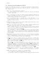
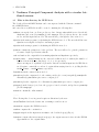
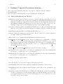
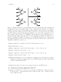
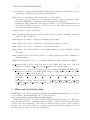
Figure 3: The three NNs used to perform NLCCA. The double-barreled NN on the left maps from
the inputs x and y to the canonical variates u and v. Starting from the left, there are l1 input x
variables, denoted by circles. The information is then mapped to the next layer (to the right)—
a ‘hidden’ layer h(x) (with l2 neurons). For input y, there are m1 neurons, followed by a hidden
layer h(y) (with m2 neurons). The mappings continued onto u and v. The cost function J forces
the correlation between u and v to be maximized. On the right side, the top NN maps from u to
a hidden layer h(u) (with l2 neurons), followed by the output layer x (with l1 neurons). The cost
function J1 minimizes the MSE of x relative to x. The third NN maps from v to a hidden layer
h(v) (with m2 neurons), followed by the output layer y (with m1 neurons). The cost function J2
minimizes the MSE of y relative to y.
costfn.m computes the cost function J for the forward map (x, y) → (u, v).
mapuv.m maps (x, y) → (u, v).
costfn1.m computes the costfn J1 for the inverse map: u → x (i.e. from u to xi).
invmapx.m computes the inverse map: u → x .
costfn2.m computes the costfn J2 for the inverse map: v → y (i.e. from v to yi).
invmapy.m computes the inverse map: v → y .
nondimen.m and dimen.m are used for scaling and descaling the data. The input are nondimensionalized according to the scaling option selected, NLCCA is then performed, and the final
results are again dimensionalized.
———
extracalc.m (optional) can be used for projecting new data onto an NLCCA mode.
4.2
Parameters stored in param.m for NLCCA
Parameters are classified into 3 categories, ‘*’ means user normally has to change the value to
fit the problem. ‘+’ means user may want to change the value, and ‘−’ means user rarely
has to change the value.
4
NLCCA
14
+ iprint = 0, 1, 2 or 3 increases the amount of printout.
Note: Printout summary from an output file (e.g. out1) can be extracted by the unix grep
command: grep # out1
− isave = 1 only saves the best solution in a .mat file, plus W and MSEx of all ensemble members.
isave = 2 saves all ensemble member solutions (more memory required).
− linear = 0 means NLCCA; linear = 1 essentially reduces to CCA. [When linear = 1, it is
recommended that the number of hidden neurons in the encoding layers be set to 1, and
testfrac be set to 0].
* nensemble is the number of members in the ensemble. (Many ensemble members may converge
to shallow local minina and hence wasted).
− testfrac = 0 does not reserve a portion of the data for testing or validation. All data used for
training. Best if data is rather clean.
testfrac > 0 (usually between 0.1 to 0.2), then a fraction of the data record will be randomly
selected as test data. Training is stopped if the MSE increases in the test data by more
than the relative threshold given by earlystop tol.
+ segmentlength = 1 if autocorrelation of the data is not of concern; otherwise the user may
want to set segmentlength to about the autocorrelation time scale.
− overfit tol is the tolerance for overfitting, should be 0 (recommended) or a small positive
number (0.1 or less). Only ensemble members having correlation of u,v over the test set no
worse than the (correlation over the training set)*(1−overfit tol), or MSE over the test set
no worse than (MSE over the training set)*(1+overfit tol) are accepted, and the selected
solution is the member with the highest correlation and lowest MSE over all the data. When
overfit tol = 0, program automatically chooses an overfit tolerence level overfit tol2 to decide
which ensemble members to accept.
− earlystop tol should be around 0.05 to 0.15. (0.1 recommended). This is the ‘early stopping’
method. Best if data is noisy, i.e. overtraining to fit the noise in the data is to be prevented.
* scaling controls scaling of the x and y variables before performing NLCCA. scaling can be
specified as a 2-element vector [scaling(1), scaling(2)], or simply as a scalar (then both
elements of the vector will take on the same scalar value).
scaling(1) = −1, no scaling (not recommended unless variables are of order 1).
scaling(1) = 0, scales all xi variables by removing the mean and dividing by the standard
deviation of each variable. [This could exaggerate the importance of the variables with small
standard deviations, leading to strange results].
scaling(1) = 1, scales all xi variables by removing the mean and dividing by the standard
deviation of the 1st x variable. (Similarly for 2, 3, ...)
Note: When the x variables are the principal components of a dataset and the 1st variable
is from the leading mode, scaling(1) = 1 is strongly preferred. [If scaling = 0, the importance
of the higher PC modes can be greatly exaggerated by the scaling].
Similarly for scaling(2) which controls the scaling of the y variables.
* penalty scales the weight penalty term in the cost function. If 0, no penalty used, while 1e−6 0.1 uses a reasonable amount of weight penalty. Increasing penalty leads to less nonlinearity
(i.e. less wiggles and zigzags when fitting to noisy data). Too large a value for penalty leads
4
NLCCA
15
to linear solutions and trivial solutions. Recommend starting with a penalty of say 0.1, then
try 0.01, 0.001, . . .
+ maxiter scales the maximum number of function iterations allowed during optimization. Start
with 1, increase if needed.
+ initRand = a positive integer, initializes the random number generator, used for generating
random initial weights.
− initwt radius controls the initial random weight radius for the ensemble Adjust this parameter
if having convergence problem. (Suggest starting with initwt radius = 1). The weight radius
is smallest for the first ensemble member, increasing by a factor of 4 when the final ensemble
member is reached.
Note: penalty, maxiter and initwt radius can each be specified as a 3-element row vector, giving the
values to be used for the forward mapping network and the two inverse mapping networks
separately. (e.g. penalty = [0.1 0.02 0.01] ). (If given as a scalar, then all 3 networks use the
same value.)
Input dimensions of the networks:
* l1 is the number of input x variables.
* m1 is the number of input y variables.
* l2 is the number of hidden neurons in the first hidden layer after the input x variables.
* m2 is the number of hidden neurons in the first hidden layer after the input y variables. For
nonlinear solutions, both l2 and m2 need to be at least 2.
Note: The total number of free (weight and bias) parameters is 2(l1 × l2 + m1 × m2) + 4(l2 +
m2) + l1 + m1 + 2. In general this number should be less than the number of samples in the
dataset. If this is not the case, principal component analysis may be needed to pre-filter
the datasets, so only the leading principal components are used as input to NLCCA.
4.3
Variables in the codes for NLCCA
The reader can skip this subsection if he/she does not intend to modify the basic code.
Global variables are given by:
global iprint isave linear nensemble testfrac segmentlength ...
overfit tol earlystop tol scaling penalty maxiter initRand ...
initwt radius options n l1 m1 l2 m2 iter xmean xstd ymean ystd...
ntrain xtrain ytrain utrain vtrain xitrain yitrain ...
ntest xtest ytest utest vtest xitest yitest corruv MSEx MSEy ...
ens accept ens accept1 ens accept2 ens corruv ens MSEx ens MSEy ...
ens W ens W1 ens W2 ens utrain ens vtrain ens xitrain ens yitrain ...
ens utest ens vtest ens xitest ens yitest
If you add or remove variables from this global list, it is CRITICAL that the same changes
are made on ALL of the following files: nlcca1.m, nlcca2.m, param.m, calcmode.m, costfn.m,
mapuv.m, costfn1.m, invmapx.m, costfn2.m, invmapy.m, extracalc.m.
5
HINTS AND TROUBLE-SHOOTING
16
n is the number of samples [automatically determined from xdata and ydata (assumed to have
equal number of samples) by the function chooseTestSet].
xdata is an l1 × n data matrix, while ydata is an m1 × n data matrix.
(A common error is to input an n × l1 data matrix for xdata, or an n × m1 matrix for ydata,
which leads MATLAB to complain about inconsistent matrix dimensions).
If xdata and ydata contain time series data, it is useful to record the measurement time in
the variables tx and ty respectively (both 1 × n vectors). The variables tx and ty are not
used by NLCCA in the calculations.
iter is the number of function iterations.
xmean and xstd are the means and standard deviations of the xi variables (Similarly, ymean and
ystd are for the yj variables).
ntrain, ntest are the number of samples for training and for testing.
xtrain, xtest are the portions of xdata used for training and testing, respectively.
ytrain, ytest are the portions of ydata used for training and testing.
utrain, utest are the canonical variate u values during training and testing. Similarly for vtrain
and vtest.
xitrain, xitest are the model predicted values for x during training and testing. (Similarly for
yitrain and yitest).
MSEx is the mean squared error of x over all data (training+testing). (Similarly for MSEy).
ens accept has value 1 if the ensemble member for the forward map passed the overfit test,
otherwise 0. Similarly, ens accept1 and ens accept2, for the 2 inverse maps.
ens corruv saves the corr(u, v) for all ensemble members. Similarly, ens MSEx, ens MSEy, ens W,
ens W1 and ens W2 save the MSEx, MSEy and the weights W, W1, W2 for the 3 NNs
respectively, for all ensemble members.
Similarly for ens utrain ens vtrain ens xitrain, ens yitrain, ens utest, ens vtest, ens xitest and
ens yitest.
When isave = 2, all the ensemble solutions, i.e. ens utrain ens vtrain ens xitrain, ens yitrain,
ens utest, ens vtest, ens xitest and ens yitest are saved. (This could increase memory usage
considerably).
5
Hints and trouble-shooting
In MATLAB 7, some of the original function M-files in the MATLAB Optimization Toolbox are no
longer available. The missing M-files can be downloaded from
http://www.ocgy.ubc.ca/projects/clim.pred/download.html.
If the data are not noisy, one can run with the weight penalty parameter(s) set to 0. With noisy
data, this will often lead to overfitting, resulting in wiggly or zigzag solutions. Increasing weight
penalty reduces the nonlinearity of the solution, resulting in smoother curves. If the penalty is
too large, one gets the linear solution, or even the trivial solution where all weights are zero (and
all data points get mapped to the same output point).
5
HINTS AND TROUBLE-SHOOTING
17
Increasing the number of hidden neurons allow more complicated nonlinear solutions to be
found, but also more chance of overfitting. One should generally follow the principle of parsimony
in that the smallest network which can do the job is the one to be favoured.
A common error message from MATLAB is: ‘Inner matrix dimensions must agree’. Use the
whos command to check the dimensions of your input data matrix xdata (ydata). For instance,
it is easy to erroneously put in an n × l data matrix for xdata in NLPCA, when it should be an
l × n matrix (i.e. the transpose).
Sometimes, the program gives the error that no ensemble member has been accepted as the
solution. One can rerun with a bigger ensemble. One can also raise overfit tol to tolerate more
overfitting. The best option may be to increase the weight penalty (and/or reduce the number of
hidden neurons) to reduce overfitting, which is usually the cause of having no ensemble members
accepted.
Sometimes, one gets the warning message about mean(u2 ) or mean(v 2 ) not close to unity.
This means the normalization terms in the cost function were not effective in keeping mean(u2 )
or mean(v 2 ) around unity. This usually occurs when large penalty were used, so the penalty terms
dwarfed the normalization term. One can either ignore the warning or scale up the normalization
term in the cost function (in invmapx.m for NLPCA, and in mapuv.m for NLCCA).
There is a known bug inside the MATLAB optimization program fmin.u. Once in a while, it
returns a ‘NaN’ (‘not a number’), presumably due to division by zero. Usually this only happens
to one of the ensemble members and does not affect the final selected solution from the ensemble.
(To check for NaN in unix, use: grep NaN output.file). If the problem affects the final solution,
simply rerun with a different value for initRand, which will generate a different set of random
initial weights.
For NLCCA, one might find the correlation to be higher than that achieved by CCA, but the
MSE to be worse than those in CCA. This means overfitting has occurred in the first network.
More penalty can be used in the first network than in the remaining two networks, e.g. penalty
= [0.1 0.02 0.01].
Finally, the most serious weakness of these nonlinear methods, namely that the number of
hidden neurons and the penalty parameters are chosen somewhat subjectively, can be largely
alleviated by using ensembles. The ensemble members can cover a range of values for number of
hidden neurons and penalty parameters. One can then choose the best 25 -30 ensemble members,
and average their solutions to yield the final solution.
5
HINTS AND TROUBLE-SHOOTING
18
References
Burnham, K.P. and Anderson, D.R. 1998. Model Selection and Inference. Springer, New York,
353 pp.
Hsieh, W.W. 2000. Nonlinear canonical correlation analysis by neural networks. Neural Networks,
13, 1095-1105.
Hsieh, W.W., 2001a. Nonlinear principal component analysis by neural networks. Tellus, 53A,
599-615.
Hsieh, W.W. 2001b. Nonlinear canonical correlation analysis of the tropical Pacific climate variability using a neural network approach. Journal of Climate, 14, 2528-2539.
Hsieh, W.W. 2004. Nonlinear multivariate and time series analysis by neural network methods.
Reviews of Geophysics, 42, RG1003, doi:10.1029/2002RG000112.
Hsieh, W.W. and A. Wu. 2002. Nonlinear multichannel singular spectrum analysis of the tropical
Pacific climate variability using a neural network approach. Journal of Geophysical Research
107(C7), 3076, DOI: 10.1029/2001JC000957.
Kirby, M.J. and Miranda, R. 1996. Circular nodes in neural networks. Neural Computation, 8,
390-402.
Kramer, M.A. 1991. Nonlinear principal component analysis using autoassociative neural networks. AIChE Journal, 37, 233-243.
von Storch, H. and Zwiers, F.W. 1999. Statistical Analysis in Climate Research. Cambridge Univ.
Pr., 484 pp.