1
User guide for 1+1D Var shallow water model
Amos S. Lawless, The University of Reading
This document provides brief documentation to run simple variational assimilation experiments on the 1D shallow water model with no rotation. This system is
essentially a simple 4D-Var system, but has just one space dimension plus a time
dimension.
1
1.1
Setting up the system
Microsoft
You are given a compressed folder SW norot.zip, copy it to the place you want
your project to live, right click on the file and select Extract All, then follow the
instructions in the WinZip wizard. If you do not have WinZip then it needs to be
downloaded and installed. It is recomended that you use a compiler with an intergrated development environment for example Salford. A free version of Salford F95
can be downloaded from: www.silverfrost.com/32/ftn95/ftn95 personal edition.asp
If you are using Salford then the Fortran project is already made for you, simply
open the file my SW.ftn95p in the top level of the new directory structure. If you
are using a different environment then you will have to select all .f and .f90 files
in directories minim, Model/fort, Model/PFM, Model/PFM Adj, Model/TLM and
var/code and add them to a new project.
1.2
UNIX
Copy the file ‘SW norot.zip’ into the directory under which you want to create your
shallow water assimilation and unzip the file with the ‘unzip’ command.
Note that this will create a directory called ‘SW norot’ in the directory in which you
unzip the file and then all other files will be under the SW norot directory. Hence
you do not need to create a special directory first.
2
Directory structure
By following the instructions in the previous section, you will automatically set up
the following directory structure under the directory SW norot.
Case 1 Contains the input variables file, ‘vars user mod test1.f90’, for example assimilation 1. All output files are found here aswell.
1
Case 2 Contains the input variables file, ‘vars user mod test2.f90’, for example assimilation 2. All output files are found here aswell.
data in Directory from which any input files will be read. By default this contains
an example input data file (nl t25.dat) and grid file (grid) for a domain of 200
points.
data out Directory into which all output will be written.
doc Contains documentation of the system.
minim Contains the minimization routine conmin.f. No other minimization routines are presently provided.
Model Contains source code for the nonlinear, linear and adjoint models, with the
following subdirectories
fort Source code for nonlinear model.
PFM Source code for perturbation forecast model.
PFM Adj Adjoint routines for PFM.
TLM Source code for tangent linear model.
TLM Adj Adjoint routines for PFM.
plot Contains Matlab routines for viewing output.
var Contains code and scripts for running the assimilation, with the following subdirectories
code Source code for assimilation scheme.
exec Default directory where code is executed.
3
3.1
Running an assimilation
Microsoft
Once you have a project set up inside the compiler’s development environment
simply click ‘build’ or ‘compile and link’, then ‘run’.
3.2
UNIX
The script to run the assimilation is called ‘Unix Compilation script.txt’ and is
found at the top of the new directory structure. To run the script simply type
’./Unix Compilation script.txt’ from the command line. It may, on some systems, be
necessary to run the command ‘dos2unix Unix Compilation script.txt’, or a similar
command, first.
2
4
Input Files - Assimilation Variables and Namelists
You are provided with two assimilation versions which use different input data and
generate different output. The input variables can be found in the files
‘Case 1/vars user mod test1.f90’ and ‘Case 2/vars user mod test2.f90’. The output
from both of these examples has also been stored in these directories. When a new
version of the assimilation is run it is recommended that you edit a copy of one of
these files and create a new directory to store it and the new output files in.
There are other input files, found in the directory ‘data in’, but these should not
be changed. The ‘vars user mod.f90’ files store all of the input data in namelists,
the variables are listed below (a default value is in brackets):
Namelist &general
This namelist controls the timing information for the assimilation and forecast.
x len Number of grid points in domain [1000]
problem number Choice of initial set up (1=Erbes data, 2=Houghton and Kasahara data, 3=Read in dataset). [3]
delta x Model spatial step [0.01]
timestep Model time step [9.2D-3]
number of assim timesteps Number of assimilation time steps [250]
number of forecast timesteps Number of forecast time steps [250]
model error Include error in all model runs except the truth, where the model
error is given by halving the size of the orography (0=Perfect model, 1=model
error) [0]
Namelist &model
This namelist controls the running of the numerical model.
linear model Linear model used in inner loop (1=Tangent linear model, 2=Perturbation forecast model) [1]
sl iterations Number of iterations for departure point calculation [3]
interp scheme Interpolation for semi-Lagrangian scheme (1=Cubic Lagrange, 2=Linear) [1]
solver diag level Level of output diagnostics for solver (0=None, 1=Residual norm,
2=Maximum and minimum values) [1]
solver max iterations Maximum number of iterations for elliptic equation solver
in model [50]
3
solver tolerance Tolerance for convergence of elliptic equation solver within model
[1.0D-8]
alpha 1, alpha 2, beta 1, beta 2 Time weighting parameters for semi-implicit
scheme [0.6]
alpha 1p, alpha 2p Extra time weighting paramteres for PF model [0.6]
phi bar Basic state φ in numerical model [1.5]
Namelist &observations
This namelist controls when and where the observations are in the assimiliation.
The variables for observations of u are listed here. Control of observations of φ are
by means of similar variables, with u replaced by phi in the variable names (eg.
first u ob timestep becomes first phi ob timestep).
first u ob timestep First time step on which observations of u are present [0]
last u ob timestep Last time step on which observations of u are present (-1
indicates till the end of the assimilation window) [-1]
time frequency of u obs Time frequency of u observations in number of time
steps [1]
first u ob point First spatial point at which there are observations of u [1]
last u ob point Last spatial point at which there are observations of u (-1 indicates
till end of domain) [-1]
space frequency of u obs Spatial frequency of u observations in number of grid
points [1]
variance of u obs If non-zero then add random noise to the observations with
specified variance [0.0D0]
Namelist &var control
This namelist controls how the assimilation is performed.
assim scheme Assimilation scheme to use (1=Incremental 4D-Var, 2=3D-FGAT,
3=Incremental 3D-Var) [1]
background setup Definition of background field (1=truth+random noise, 2=constant, 3=truth with phase error, 4=zero everywhere) [1]
variance of u background Variance of random noise to add to u to form background if background setup=1. Also used as variance if cov B matrix=3
[0.0D0]
variance of phi background Variance of random noise to add to φ to form background if background setup=1. Also used as variance if cov B matrix=3
[0.0D0]
4
corr length Correlation length in number of grid points if cov B matrix=3 [1].
max number of outer loops Maximum number of outer loops to perform [1]
minim diag Controls output from minimization (0=No printed output from minimization, > 1 = Values written out every minim diag iterations) [1]
minim max iterations Maximum number of minimization iterations to perform
in each inner loop [Default 50]
cov B matrix Specification of background error covariance matrix (1=Zero, ie.
ignore this term, 2=Identity, 3=Laplace operator) [2]
cov R matrix Specification of observation error covariance matrix (1=Zero, ie.
ignore this term, 2=Identity, 3=True error variance) [2]
filter steps If > 1 then the increment is added on to the linearization state over
this number of time steps, to provide a simple filter [1]
stop criteria Choose which criteria to stop the inner loop on (1=Relative gradient,
2=Absolute gradient, 3=Relative change in function, 4=Gradient relative to
initial gradient) [1]
low res factor Ratio of outer loop: inner loop spatial resolution [1]
inner tolerance Stopping tolerance for inner loop [1.0D-6]
outer tolerance Stopping tolerance for outer loop. Note that the outer loop stops
when the absolute norm of the gradient is less than this tolerance [1.0d-6]
mach accuracy Estimate of machine accuracy, used in CONMIN routine [10.D-20]
Namelists &diags and &luns
The variables in these namelists set up the output files and so in general should not
be changed. The only one which may be of use is the variable L gradient test in the
namelist &diags. If this is set to .true. then the gradient test is run instead of the
assimilation. The default is false.
5
Output Files
The output data files used are found in the directory ‘data out’ and their apperance
in the code is in the file ‘main.f’; you may wish to rename the outputs. The output
files are as follows:
outfile.dat A text file which shows all of the standard output information as the
code runs. At the end of this file there is the number of points required for
making the plots with the Matlab scripts.
costfn.dat Iterations of the cost function and gradient for plotting using routines
conv.m and convt.m.
5
analysis.dat Analysis data file for plotting using routines plotanal.m and plotanal2.m.
background.dat Background data file.
truth.dat Truth data file.
These files will be overwritten every time the code runs, so if they are to be stored
they should be renamed or moved elsewhere, for example in the same directory
where your edited input variable file ‘vars user mod.f90’ lives.
6
Plotting the output using Matlab
6.1
Plotting Routines
The routines for plotting output can be found in the directory plot. There are four
routines.
conv.m
This routine plots the cost function and gradient convergence for a given run, using
the costfn.dat output file. The user should set the variable data dir at the top of the
routine to the directory of where the output files of the run are held and the name
of the costfn.dat file to be read. The routine is then called using the command
conv(N)
where N is the number of lines in the costfn.dat file written out during the minimization process. This number is printed out at the end of the corresponding output.dat
file.
conv2.m
This routine works in exactly the same way as conv.m, but allows the convergence
of two runs to be compared, for example one with a TLM and one with a PFM.
The user must now set two directory paths at the top of the routine, data dir and
data dir2, and the routine is called using the command
conv(M,N)
where M and N are the numbers described above for the respective runs.
plotanal.m
This routine plots the truth, background and analysis at various times throughout
the run. The user must set the following options at the top of the routine:
• number of times: The number of output times to plot.
• times: A vector consisting of the output times to plot (Units: time steps).
• data dir : Full pathname of data directory.
6
The name of the analysis file also needs to be specified. The output consistes of two
figures. Figure 1 shows a comparison of the truth, background and analysis for the
u and φ fields at the times requested. The truth is shown by a black solid line, the
background by a red solid line and the analysis by a black dashed line. Figure 2
shows the error in each of the fields (truth-analysis).
N.B. If you have set the background term to zero in your analysis (cov B matrix=1)
then you should comment out the plotting of the background field.
plotanal2.m
This routine works in exactly the same way as plotanal.m, but allows comparison
from two different assimilations. The only difference in the set up now is that the
user must specify two data directories at the start of the routine. The output is the
same as previously, with the extra analysis being indicated by a black dotted line.
6.2
Example Plots
The routines conv.m and plotanal.m are used to make example plots for the test
cases 1 and 2, and can be found in the corresponding directories.
Figure 1: The cost function convergence for input test case 1.
7
Figure 2: The cost function convergence for input test case 2.
8
Figure 3: A comparison of the truth, background and analysis for the u and φ fields
for test case 1. Truth: black solid line. Background: red solid line. Analysis: black
dashed line.
9
Figure 4: The error in the u and φ fields for test case 1. Truth: black solid line.
Analysis: black dashed line.
10
Figure 5: A comparison of the truth, background and analysis for the u and φ fields
for test case 2. Truth: black solid line. Background: red solid line. Analysis: black
dashed line.
11
Figure 6: The error in the u and φ fields for test case 2. Truth: black solid line.
Analysis: black dashed line.
12