1
Beginners Guide to Khepera Robot Soccer
Narongdech Keeratipranon and Joaquin Sitte
Smart Devices Lab
School of Software Engineering and Data Communications
Queensland University of Technology
Brisbane, Qld, Australia
e-mail: [email protected]
Brisbane 2003
1
Section 1
Introduction
The purpose of this guide is provide initial help for setting up Khepera robots to play an
autonomous simplified game of soccer whether it is just for the fun of it or for participating in
the Kheperasot robot soccer tournament organized by the Federation of International Robotsoccer Association (FIRA). This guide has the following sections: FIRA Kheperasot game
rules. The Khepera robot soccer facility consists set up a Khepera robot soccer environment
consists of a playing field, robot-computer communication, and software development.
1.1
Background
Playing a soccer-like game with small mobile robots is not only great fun for technology fans
but also great technical challenge and educational experience. Numerous categories are open to
competitors under the umbrella of two international championships: the RoboCup and the
FIRA World Cup.
The various leagues are quite demanding though in terms of resources and effort required from
the participants. Often quite sophisticated robots have to be built. Five or more of them are
required for a team and the playing fields are of the size of small room. In many cases powerful
computer vision are required. Not surprisingly teams of advanced undergraduate and
postgraduate engineering students from universities dominate the tournaments.
The Kheperasot (http://www.fira.net) league from FIRA (Federation of International RobotSoccer Associations) offers a challenging game yet the entry cost is significantly lower than
for most other leagues. There is no need to build robots as the Khepera robots are commercially
available general purpose research robots. A Khepera robot is of the size of a small coffee cup
and thus the playing field can be small enough to fit on a desk or table. There is no expensive
external vision system and no wireless communication. In its simplest form only one robot is
needed per team. The technical challenge in this league resides in programming the robots to
play a truly autonomy of soccer playing robots. Once a robot is let loose on the playing field it
has to fend with its own sensors and computing resources. The robot has be capable of locating
itself in a simplified environment, recognize landmarks (goals) and other moving objects (ball,
opponent) and move quickly and purposefully to outsmart the adversary. And it has to achieve
all this with the sensing and computing devices fitting in such a small robot. A C programming
environment and two simulators support software development. Creating a moderately
competent player is within the reach of a two student team in couple of weeks and is suitable
as a practical semester assignment in an embedded systems programming, control or
computational intelligence course.
Khepera is a miniature robot originally designed as a research and teaching tool in the Swiss
Research Priority Program. It was first implemented in 1992, by a research team from the
Microprocessor and Interface Laboratory (LAMI) at the Swiss Federal Institute of
Technology, Lausanne (EPFL) and is currently developed by K-TEAM SA, Switzerland. The
Khepera robot is now widely used around the world as a platform for various robotics
experiments and applications. Researchers can easily extend Khepera’s capability by
attaching it with additional desired modules such as a gripper module, video module or linear
2
vision module. It has two motor driven wheels and is equipped with 8 infra-red sensors
allowing it to detect obstacles all around it in a range of about 5 cm.
The Khepera robot is a two wheeled robot with a cylindrical shape 70 mm in diameter and 30
mm high. The robot has 8 infra-red proximity sensors, two independent motors for differential
steering and two encoders to measure wheel rotation. Because there are several expansion
modules, called turrets, that can be stacked on the top of the Khepera robot the bare Khepera
robot is also called the Khepera base,.
Proximity sensors alone are not enough to allow the robot to play a soccer game. The K213
linear camera turret provides simple vision capability enough to perceive objects at a distance.
The linear camera has a detector with 64 pixels arranged along a horizontal line. Each pixel
gives 256 gray-levels. Thus the linear camera produces an image of the light intensity along a
horizontal line in the scene covering 36 degrees. The limited amount of visual data can be
processed by the microprocessor on the Khepera enabling autonomous operation.
The line scanned by the camera is about 50 mm above the ground. For a ball to be seen its
diameter has to be larger than this height. For this reason a tennis ball is used as soccer ball.
The colour is bright yellow to make it easier to discriminate from the other object in the
playing field. To make it easier to distinguish the opponent robot from the ball the robots are
dressed with a jerse, which is simply a paper cylinder with alternating black and white stripes.
The goals are painted black inside to distinguish them from the walls of the playing field
which are painted in a medium shade grey.
Section 2
The K213 linear vision turret
Because the key role of the vision sensor we start by describing the characteristics of the
linear camera useful for recognising the ball, the goals, and the opponent robot and for
determining the robot's position in the playing field.
2.1 Output from the Linear Camera
The K213 linear camera can provide up to 64 pixels in horizontal line with 256 grey-scale
with a variable frame rate of a maximum of 5 Hz. The angle of view is 36 degrees. The optics
of the camera is fixed and set for objects between 50 and 500 mm to be in focus. However
considering that one pixel covers 0.5 of a degree which at 500 mm makes 4.3 mm on can see
that resolution is set by the number of pixels and not by the focus. There is not noticeable
deterioration of resolution well beyond 500 mm distance.
The linear photosensor array (TSL213) consists of 64 discrete photo sensing areas called
pixels.. Photons striking a pixel generates a charge in the region under the pixel. The amount
of charge accumulated in each element is directly proportional to the amount of incident light
and the integration time. After the integration period is finish, the signals in each pixels are
transferred to the TSL213 output, and the charge values in each pixels are reset.
Normally, a pixel from a bright object will give a higher value than a dark object. The bright
tennis ball should give the highest value follow by the grey wall, and the black goal will be
3
the lowest. However if the scene is very bright all pixels could have a high value and the
brighter parts could make the pixels saturate.
To maintain the image contrast over a wider range of scene brightness the K213 linear vision
also has ambient light sensor (TSL230). The ambient light sensor controls the exposure, that
is, the time available for integrating the light incident the photosensitive array. The function
of TSL230 is to control the scanning speed to TSL213 to suit the current lighting condition.
The more ambient light, the shorter scanning speed to prevent the saturation of photo sensing
elements in TSL213. Such as at the goal region which has a less light than the wall region, the
frequency output from the TSL230 will lesser, that mean the TSL213 will use more time to
collect the image information and smaller differences in the low light intensity area will be
enhanced.
Unfortunately the usefulness of this exposure control method greatly diminished by what
seems to be a design fault. The problem is that the aperture of the ambient light sensor is not a
narrow slit corresponding to the linear camera but a cone of approximately the same hight and
width. Thus the brightness of the scene above and below the line scanned by the TSl213 will
contribute to the ambient light signal. For example a light background above the goal will
keep the scan rate higher than desired. From this reason, it has been found that it is better to
disable the adaptive scanning frequency from TSL230 and use a constant frame rate all over
the playing field.
To get a constant frame rate we need to send a constant frequency to TSL213. Two effective
solutions are available to accomplish this. First, a normal LED will be attached in the ambient
light aperture to provide constant illumination of the TSL230. The second solution is to
replace the TSL230 with an adjustable frequency oscillator and feed the output into the
TSL213. These modifcationa are described in detail in section 2.4 below. The LED solution is
easy to implement and gives good results.
A further advantage of disabling the automatic scan rate control is that the scan rate can be
adjusted fit the overall illumination level, for example when setting up the playing field in a
different place.
2.2 Typical Images
This section will provide examples of output received from the linear camera in both original
and modification case, additional light and normal ambient light, near and far from the
objects, and also with different soccer objects.
We will set the variable resistance of LED circuit to 55k Ω if only normal ambient light is
used ( a photo meter measured 200 lux at this condition. ) And will set the variable resistance
to 40k Ω in case of using additional 150 W halogen light ( a photo meter measured 500 lux at
this condition. )
We will use three distances, 10, 30, and 50 centimetres away from the objects, to test the
robot vision.
4
We used following situations to test the camera
1 The ball in front of the wall, the results are shown in Figure 2 – 1.
2 The ball in front of the goal, the results are shown in Figure 2 – 2.
3 The ball in front of the wall and the goal, the results are shown in Figure 2 – 3.
4 The opponent robot in front of the wall, the results are shown in Figure 2 – 4.
5 The opponent robot in front of the goal, the results are shown in Figure 2 – 5.
6 The opponent robot in front of the wall and the goal, the results are shown in
Figure 2 – 6.
7 The ball and the opponent in front of the wall, the results are shown in Figure 2 –
7.
8 The ball and the opponent in front of the goal, the results are shown in Figure 2 –
8.
9 The ball and the opponent in front of the wall and the goal, the results are shown in
Figure 2 – 9.
In Figure 2 – 1 to Figure 2 – 9, different lines style will correspond to the different distances
from the object as shown below.
10 centimeters apart from the object
30 centimeters apart from the object
50 centimeters apart from the object
In Figure 2 – 1 to Figure 2 – 9, subfigures (a) display the location of the objects in the playing
field corresponding to each situation. Subfigures (b) are display the images when using the
modified turret with addition halogen light. Subfigures (c) display the images when using the
modified turret with normal ambient light. Subfigures (d) display the images when using the
original turret with addition halogen light. Subfigures (f) display the images when using the
original turret with normal ambient light. Subfigures (g) display the results when applying
noise filtering to the image of subfigure (b) using mode method with mask sizes 3, 5, and 7.
5
(b) Modified turret, additional light
10 cm
30 cm
50 cm
(a) Playing field situation
(c) Modified turret, normal light
(d) Original turret, additional light
(e) Original turret, normal light
(f) Noise filtering from figure (b)
Figure 2 – 1 The image received from situation 1, the ball in front of the wall.
6
10 cm
30 cm
50 cm
(b) Modified turret, additional light
(a) Playing field situation
(c) Modified turret, normal light
(d) Original turret, additional light
(e) Original turret, normal light
(f) Noise filtering from figure (b)
Figure 2 – 2 The image received from situation 2, the ball in front of the goal.
7
10 cm
30 cm
50 cm
(b) Modified turret, additional light
(a) Playing field situation
(c) Modified turret, normal light
(d) Original turret, additional light
(e) Original turret, normal light
(f) Noise filtering from figure (b)
Figure 2 – 3 The image received from situation 3, the ball in front of the wall and the goal.
8
(b) Modified turret, additional light
10 cm
30 cm
50 cm
(a) Playing field situation
(c) Modified turret, normal light
(d) Original turret, additional light
(e) Original turret, normal light
(f) Noise filtering from figure (b)
Figure 2 – 4 The image received from situation 4, the opponent in front of the wall.
9
10 cm
30 cm
50 cm
(b) Modified turret, additional light
(a) Playing field situation
(c) Modified turret, normal light
(d) Original turret, additional light
(e) Original turret, normal light
(f) Noise filtering from figure (b)
Figure 2 – 5 The image received from situation 5, the opponent in front of the goal.
10
10 cm
30 cm
50 cm
(b) Modified turret, additional light
(a) Playing field situation
(c) Modified turret, normal light
(d) Original turret, additional light
(e) Original turret, normal light
(f) Noise filtering from figure (b)
Figure 2 – 6 The image received from situation 6, the opponent in front of the wall and the goal.
11
(b) Modified turret, additional light
10 cm
30 cm
50 cm
(a) Playing field situation
(c) Modified turret, normal light
(d) Original turret, additional light
(e) Original turret, normal light
(f) Noise filtering from figure (b)
Figure 2 – 7 The image received from situation 7, the ball and the opponent in front of the wall.
12
10 cm
30 cm
50 cm
(b) Modified turret, additional light
(a) Playing field situation
(c) Modified turret, normal light
(d) Original turret, additional light
(e) Original turret, normal light
(f) Noise filtering from figure (b)
Figure 2 – 8 The image received from situation 8, the ball and the opponent in front of the goal.
13
10 cm
30 cm
50 cm
(b) Modified turret, additional light
(a) Playing field situation
(c) Modified turret, normal light
(d) Original turret, additional light
(e) Original turret, normal light
(f) Noise filtering from figure (b)
Figure 2 – 9 The image received from situation 9, the ball and the opponent in front of the wall and the goal.
14
2.3 Panoramic Images
This section will provide examples of panoramic image received from the modified linear
camera with additional 150 W halogen light in different positions over the playing field.
The panoramic image received by taking the image at the front then rotate 36 degrees
clockwise direction and take a new image, the robot will iterate this action until rotated 360
degrees around itself.
The situations that we used to test the vision were
1 The robot stands at the centre of the playing field, turned to the side wall, and the ball
is at the back. The results are shown in Figure 2 – 10.
2 The robot has pushed the ball until stuck at the opponent wall. The results are shown
in Figure 2 – 11.
3 The ball is at the centre and the robot facing the opponent goal direction. The results
are shown in Figure 2 – 12.
15
Figure 2 – 10 The panoramic image received from situation 1.
16
Figure 2 – 11 The panoramic image received from situation 2.
17
Figure 2 – 12 The panoramic image received from situation 3.
18
2.4 Vision Turret Modifications
As mentioned earlier the automatic control of the frame rate of the K213 turret is a nuisance
rather than an asset for robot soccer and it should be turned off.
To achieve this task we need to send a constant frequency to the linear light sensor chip,
TSL213. Two effective solutions are available to accomplish this. First, a normal LED will be
attached in the ambient light aperture to give constant illumination to the TSL230. The
second solution is to replace the TSL230 with an adjustable frequency oscillator and use the
output from the oscillator to control the scan rate of the TSL213.
(a) LED solution
For the LED approach we can use a simple LED circuit with variable resistors. This circuit
will provide varying brightness according to the current value of a set of resistors. A sample
of LED circuit is shown in figure C – 2. This circuit has a 270 Ω fixed resistor and two
variable resistors, 50k Ω and 5k Ω. Having two variable resistors will easier to settle
brightness as compared with only one variable resistor.
To use this LED circuit with the vision turret, we need to connect ground and Vcc to pin 2
and 5 of the outer pin of K213 turret respectively. The first pin is on the left side when
looking from the back of the camera as shown in figure C – 3. In fact we can connect the
ground of the LED circuit to any ground pin, 4, of the TSL230 or pin 6 or 7 of the TSL213
and also can connect the Vcc to any Vcc pin, 5, of the TSL230 or pin 4 or 8 of the TSL213 as
shown in figure C – 4. For the example in figure C – 3, we connect ground to pin 6 of
TSL213 and connect Vcc to pin 5 of TSL230.
After connecting the circuit with K213, we have to put the LED in TSL230 hole and block it
with black electrical tape to make the LED stable and prevent intervention between LED and
environmental light. For the tuning process, we should set a 5k resistor to approximately 2.5k
then using a 50k resistor as a rough tuning and 5k as a fine tuning.
VCC (pin 5 of the turret which
is pin 5 of TSL230)
R=270Ω
Variable R = 0-50kΩ
Variable R = 0-5kΩ
LED
GND (pin 2 of the turret which
is pin 6 of TSL213)
Figure 2 – 13 LED circuit with two variable resistors
19
Figure 2 – 14 Connect LED circuit with K213 vision turret
Figure 2 – 15 Schematic of K213
20
(b) Oscillator solution
For this solution, we can use a 555 oscillator circuit with variable resistors. This circuit will
overtake a function of TSL230, create a refresh rate signal, and will send the output directly to
TSL213. From this concept, we can achieve any refresh rate of K213 by varying the value of
a resistors. A sample of an oscillator circuit is shown in figure 2 – 16, this circuit has a 100k
Ω variable resistors. The output frequency from the oscillator can compute by using equation
2–1
1.44
f =
(2–1)
(R1 + 2 × R 2) × C
From the equation, we can select any desired-frequency by tuning variable resistor. Table 2 –
1 show the major frequencies and their correspondent resistor values.
Table 2 – 4 Oscillator frequencies and value of variable resistors
Frequency ( Hz )
102
Variable resistor ( k Ω)
0
10
To use this oscillator circuit with the vision turret, we need to remove the TSL230 chip from
the camera and connect ground, Vcc, and output of oscillator circuit to pin 4, 5, and 7 of the
inner pin of K213 turret respectively. The first pin is on the right side when looking at the
back of the camera ( opposite of the LED solution where the first pin is on the left side. ) If
we look at schematic of TSL213 and TSL230 in Figure C – 4, we connect ground to pin 4 of
TSL213, Vcc to pin 5 of TSL230, and output to pin 6.
To remove TSL230 chip, first we need to take the black plastic case around the sensors off.
The case is fixed on the PCB with a soft silicone joint. We need to cut gently through this
joint using a slim cutting tool. After this, we can easily remove TSL230 from its socket.
21
Figure C – 16 Oscillator circuit with one variable resistor
22
2.5 Keperasot robot jersey template
23
Section 3
Set up and Using Khepera
The Khepera robot can operate with or without a connection cable, execute received over the
serial connection or executed program downloaded program and use an internal or external
power source. Khepera can also be used with text-mode terminal program or use with Matlab
or LabVIEW, which can provide a nice graphic user interface.
3.1 Configuration for Robot-Computer Communication
Download a program to the Khepera robot we need to connect it a host computer. The host
computer will send any commands to the Khepera through a serial link using a standard
RS232 line, while the interface module converts the RS232 signal into an S serial signal to
communicate with the robot. In another way, the robot also sends back any information via S
serial signal and will be converted to RS232 signal by the interface module.
From the above description, the robot-computer communication system is composed of
mainly six components
- Host computer
- Standard RS232 cable
- Interface module
- S serial cable
- AC/DC adapter power supply
- Khepera
Figure 3 – 1 shows the configuration for communication between the Robot and a host
computer. If we want to use an internal battery power we can neglect AD/DC adapter
connection and set the battery switch to ON position. In general, we only use internal battery
when working in fully-autonomous mode.
Figure 3 – 1 Configuration for communication between the Robot and a host computer
3.2 Running Modes of Khepera II
A Khepera can be set to work in many configuration modes such as serial communication, S
loader or user application. Different modes will have different operations and also different
24
methods to handle. We can simply set a Khepera II mode by tuning an encoding wheel on the
top of the Khepera to one of the sixteen modes. The sixteen modes of the Khepera II can be
divided into 4 main modes which are serial communication, S loader, user application and
supporting mode. Table 3 – 1 summarizes the available modes for the Khepera II.
3.2.1 Serial communication mode
This mode is designed to control all Khepera’s functions using a RS232 serial line. The host
computer and the Khepera robot are communicating with ASCII messages. Each single
interaction is composed of
- A command, begin with one or two ASCII capital letters and followed, if
necessary, by numerical or literal parameters separated by a comma and
terminated by a carriage return or a line feed, sent by the host computer to the
Khepera robot.
- A response, beginning with the same one or two ASCII letters of the command but
in lower case and followed, if necessary, by numerical or literal parameters
separated by a coma and terminated by a carriage return and a line feed, sent by
the Khepera to the host computer.
The commands which the host computer can send to the Khepera are of two different types
- Tool command, used to set up the robot configuration from the host computer such
as the “serial” command use to set a speed for the serial line communication or
“memory” command will show the system’s memory usage.
- Control protocol, used to set controls and request sensors value form the robot
such as set the motor speeds, read proximity sensor values.
3.2.2 S loader mode
The S loader mode is used to load any user application into the robots RAM and execute it
when finished downloading. Two different methods are available to start the S loader. First,
when booting the Khepera in the S loader . Second, booting in serial communication mode
and sent the command “run sloader”.
Once started, the S loader simply waits for an executable file to be transferred through the
serial line. Different terminal emulators will have different methods to send a file but the most
common is to use a “send file” command from the terminal emulator. As soon as the loading
process is initiated, one of the Khepera's LED indicator is switched on. The indicator should
stay on during the entire loading process and be turned off when the download is completed.
The downloaded application is executed as soon as the transfer is achieved.
3.2.3 User application mode
This mode is used for a completely autonomous execution of a user application. The
application has to be uploaded in the robot's non volatile memory, using a serial link, and can
be executed at boot time.
25
To upload an application in non volatile memory, the instructions below have to be followed
- Set the robot to serial communication mode
- Use the “sfill” command to start the loader. The message “S format Motorola
loader mode” should be displayed
- Send the application file to the serial line, the same way as using in S loader mode.
As soon as the transfer is in progress, an LED indicator is switched on, and will
stay on until the transfer is completed. The application is transferred into the
robot's RAM, and still needs to be flashed. When completed, the message “S:
download terminated” should be displayed
- Erase the robot's non volatile memory using the “flash E” command. When
completed, the message “FLASH user segments erased” should be displayed
- Write the application into the flash memory using the “flash W” command. When
completed the message “FLASH user segments written” should be displayed
After uploading the application into non volatile memory, it will stay there until it is erased,
using the “flash E” command. The loaded application can be executed at any time using one
of the two following methods;
- If a serial communication link is already up, we can use the command “run userflash” to execute the user flash segment. The messages “Run the selected
application...” and “Execute a user FLASH application” should be displayed.
- For a completely autonomous execution, set the encoding wheel position to the
user application mode and reset the robot. The user flash segment is automatically
executed at boot time.
3.2.4 Supporting mode
This mode is an additional mode to support usage of the Khepera. The supporting modes are;
- Demonstration mode : Braitenberg vehicle algorithm for obstacle avoidance.
- Test mode: Successive tests are performed and the results are displayed using the
serial link.
- Flash Erasing mode : The user segment of the non volatile memory is erased.
- uKos upgrade mode: Khepera BIOS upgrade mode.
_
26
Table 3 – 1 summarized the available modes of Khepera II
Mode
User
application
Mode
Number
1
2
3
8
9
5
6
A
4
B
Supporting
0
Serial
communication
S loader
Baud rate
(bits/s)
9600
19200
38400
57600
115200
9600
38400
57600
9600
57600
Description
Mode to control the robot using the Serial
communication protocol. The robot should be
connected to a terminal using the S cable.
Robot waits for an application to be transferred
in RAM and executes it when fully uploaded.
Start an application stored in the robot's non
volatile memory. The application should be
flashed first using the S loader.
9600 Demonstration mode for Braitenberg vehicle
algorithm for obstacle avoidance.
Test mode, successive tests are performed and
the results are displayed using the serial link.
38400 Flash Erasing mode, The user segment of the
non volatile memory is erased.
38400 Khepera BIOS upgrade mode.
Reserved
7
E
_
F
C,D
The serial link set up is always 8 bit, 1 start bit, 2 stop bit, no parity. Only the baud rate can be
changed. The encoding wheel position can be changed at any time. If the robot is running, a
reset is necessary for the set up to be effective. The reset button can be used at any time to
reset the robot.
_
_
3.3 Installation and Using KTProject Package
As we mention above in section 3.2, the Khepera robot has the ability to run fully autonomous
by executing the program in its RAM or flash memory. Executable files which can be loaded
into the Khepera have to be compiled and converted into Motorola S format. K-Team
provides a GNU C cross-compiler, and the KTProject, interface which can generate the
executable files.
KTProject is a graphical C development environment for Windows platform. This package
provides a library of all the low-level functions for Khepera and its extension turrets including
motor control, sensor reading, communication, multi-tasking management, and linear camera
reading. The package also includes the GNU C compiler, the Cygwin Environment (copyright
RedHat Inc.), Source Navigator (copyright RedHat Inc.), KTDebug, and serial port terminal
Tera Term Pro.
27
3.3.1 KTProject Step-by-step Installation Guide
Information in this section is based on KTProject Version 2.2 by P.Bureau, K-Team 2002.
The package is self executable, 26Mb, compatible with Windows 32bits environment ( such
as Win 95, 98, 98SE, Me, NT, 2000 and XP ) and can be downloaded for free at ftp://ftp.kteam.com/pub/cross-compiler/KTProject/KTProject.exe.
After downloading KTProject 2.2, double click on the download file. The complete download
version is called KTProject.exe
Step 1: Confirmation of Installation
Set up package will ask to confirm installation KTProject, click Yes.
Step 2: Greeting Message
This screen will provide a greeting message and some recommendations to close all
applications before continuing, click Next.
Step 3: Destination Direction
28
This screen will ask the folder where it will keep the KTProject application. We recommend
to keep the destination direction as it was, in this case C:\Program Files\KTProject, thus
reducing the trouble for future assistance from any other sources, click Next.
Step 4: Start Menu Folder
This screen will ask for the start menu folder name. We recommend to keep the folder name
as it was, in this case KTProject, click Next.
29
Step 5: Select Additional Task
This screen will ask what additional tasks should be performed. In this case it only has one
option, create a desktop icon, that should be ticked, then click Next.
Step 6: Confirmation
This screen will summarize what is going to be installed, if everything is correct then click
Install.
Step 7: Progress of Installation
The installation has begun and KTProject will be ready to launch soon.
30
Step 8: Finish
The installation package will show the completed installation screen, click Finish
3.3.2 Using KTProject
After installation is finished we will get the start menu group KTProject which provide the
short cut to KTProject and the short cut to Uninstall KTProject.
31
We also get a short cut to "C:\Program Files\KTProject\KTProject\KtProject.exe" on a
desktop.
.
We now show step-by-step below how to use KTProject by demonstrating opening and
compiling an example in the package. First execute KtProject.exe ( please not confuse with
installation package KTProject.exe ) by double click on the desktop icon, click on the short
cut menu, or directly select "C:\Program Files\KTProject\KTProject\KtProject.exe"
Step 1: Choose project option
This screen will ask whether to create a new project or open an existing project. For both
creating and opening a project task it is better to choose an “Open Existing Project” option.
The reason forI not useing “Create New Project” option is that the software tends to crash and
needs to be reopened when trying to create a new project by using an available example file
but the problem does not occur when using “Open Existing Project” option. Click “Open
Existing Project”
Step 2: Source-Navigator Projects Control Menu
This screen will display all projects which already opened from current machine. In this case
no project was opened, therefore no projects are display on the screen.
- “New Project” is use to create a new project from an existing source file or create
from a template file.
- “Browse” is use to select an existing project which never opened from current
machine.
32
“Open” is use to open an existing project which already opened from current
machine, the button will be active when we selected any project in the list box on
the left.
- “Delete” is use to delete selected project in the list box on the left.
Our objective is to create a new project from existing source file then click “New Project”
-
Step 3: Create Project
This screen will provide an easy way to create a new project. In this example, we will create a
project from an existing example, Braitenberg vehicle obstacle avoidance algorithm, using
Khepera II robot.
First, we need to provide the new project file name and its path. Click “…” next to the
text box of Project File, when the open dialog has poped-up change the directory to
“C:\Program Files\KTProject\kh2pack601\examples\braiten” and input “braiten.proj” in the
File name text box. Then click “Save”.
Second, in Add Directory text box we need to provide the project directory which is
“C:\Program Files\KTProject\kh2pack601\examples\braiten”.
Third, we need to copy a “Makefile”, a file that contains compilation options, from
“C:\Program Files\KTProject\kh2pack601\examples\Makefile” which has the suitable options
for Khepera II into
“C:\Program Files\KTProject\kh2pack601\examples\braiten”.
To do this we can use any file management program such as Windows Explorer.
When you have finish these three steps, click “OK” button.
33
Step 4: Source-Navigator Symbols Main Menu
This screen will provide information of the current project and also detail of each files. More
information on how to use Source-Navigator please consult Online manual by clicking at
Help menu and then Online manuals.
To modify some source code we can double click on that particular file.
Step 5: Source Code Editor
34
This screen will display the source code of desired file. We can modify any code directly via
this interface. More information on how to write C-Code for Khepera II please consult
Khepera II programming manual and Khepera BIOS reference manual (http://www.kteam.com/download/khepera/documentation/Kh2ProgrammingManual.pdf,
http://www.kteam.com/download/khepera/documentation/KheperaBIOSRefManual.pdf )
To compile a project click on the menu bar Tools -> Build from Source-Navigator Symbols
Main Menu Window or Source Code Editor Window.
35
Step 6: Build Main Menu
We will use this screen use to compile and build a project file into a Motorola S format. Any
error messages or instruction guide will display in the list box below. More information for
Motorola S format please consult appendix C of Motorola M68000PRM manual (ewww.motorola.com/collateral/M68000PRM.pdf )
To create a Motorola S format ( *.s37 ) click “Start”
After finishing these 6 steps, if we look in the main project directory “C:\Program
Files\KTProject\kh2pack601\examples\braiten” will have
-
braiten.c
braiten.o
braiten.proj
braiten.s37
-
Makefile
.snprj
a source file
an object file
a project file
an executable file in Motorola S format which will be
downloaded into Khepera
a compilation script file
a directory used in the compilation process
36
3.4 Using Tera Term Pro
Tera Term Pro is a free terminal emulator for Microsoft-Windows operating systems. The
emulator is included in KTProject package and will be installed in directory “C:\Program
Files\KTProject\Kterm”. Tera Term Pro can used to communicate with Khepera in every
running mode. Before using the emulator, the serial link between the host computer and the
robot has to be properly configured. Please refer to section 3.1 for a detailed description of
necessary connections and configuration.
We will show step-by-step below how to use Tera Term Pro to communicate with Khepera.
More information in using Tera Term Pro please refer to Tera Term Pro homepage (
http://hp.vector.co.jp/authors/VA002416/teraterm.html ). First execute “C:\Program
Files\KTProject\Kterm\ttermpro.exe”
Step 1: Choose connection type
This screen will ask the connection type, to connect with Khepera select Serial and choose the
connect communication port. Click “OK”
Step 2: Serial port setup
To set up serial port click Setup Æ Serial port. This screen will use to configure serial port
property according to Khepera mode.
- Port, select according to current connection port
- Baud rate, select according to Khepera mode ( please refer to section 3.2 ), in this
case using mode 8, serial communication with baud rate 57600.
- Data, always set to 8 bits
- Parity, always set to none
- Stop, always se to 2
- Flow control and transmit delay, use its default values
37
Step 3: Main screen of Tera Term Pro
After finishing with setting up the serial port, press reset button of the Khepera. The screen
should look like figure below ( this example the running mode is set to mode 8, serial
communication )
Step 4: Terminal setup
To work in serial communication mode, we better enable “Local echo” function because we
will able to see the command we typed. To open the terminal setup screen, click Setup Æ
Terminal. If we want to enable “Local echo” property check the box in front of “Local echo”.
38
Step 5: Test some protocol commands
Now we are ready to communicate with Khepera II via the serial link. Below is a sample of
protocol command for the Khepera II.
-
Type the capital letter B followed by a carriage return or a line feed.
The robot must respond with b followed by an indication of the version of
software running on the robot and terminated by a line feed.
Type the capital letter N followed by a carriage return or a line feed.
The robot must respond with n followed by 8 numbers separated by a comma and
terminated by a line feed. These numbers are the values of the robot proximity
sensors.
Retry the same command (N) putting some obstacles in front of the robot. The
response must change.
Type the protocol command D,5,-5 followed by a carriage return or a line feed.
The robot must start turning on the spot and respond with d and a line feed.
To stop the robot type the protocol command D,0,0 followed by a carriage return
or a line feed.
Type the protocol command H followed by a carriage return or a line feed.
The robot must respond with h followed by 2 numbers separated by a comma and
terminated by a line feed. These numbers are the values of the position counters of
each wheel.
Type the protocol command G,0,0 followed by a carriage return or a line feed.
This command set the position counters to the 2 values given as parameters. The
answer is composed by a g and a line feed.
Retry the protocol command H to verify that the G command has been executed.
Type the protocol command C,1000,1000 followed by a carriage return or a line
feed.
The robot respond with c and goes forward 80 mm.
Retry the protocol command H to verify the final position.
39
For more protocol commands please refer to appendix A of Khepera II user manual
(http://www.k-team.com/download/khepera/documentation/Kh2UserManual.pdf )
Step 6: Test to send executable file in Motorola S format ( *.s37 )
Before we can send any files to the Khepera, we have to change the running mode to S loader
mode. Two different methods are available to start the S loader. First, when booting the
Khepera in the S loader mode ( please refer to Table 3 – 1 ). Second, booting in serial
communication mode and command “run sloader”.
Currently we are`already in serial communication mode then type “run sloader”. After typing
the command, the messages “Run the selected application…” and “S format Motorola loader
mode” should display, we have to select the file we want to send in this case will use
Æ
Send
file
and
then
select
“C:\Program
“braiten.s37”.
Click
File
Files\KTProject\kh2pack601\examples\braiten\braiten.s37” which we receive after building
braiten project ( to build a project please refer to section 3.3 ). The download dialog will popup while downloading the file. The downloaded application is executed as soon as the transfer
is achieved. In this case the Khepera will move around and avoid any obstacles ( please put
the Khepera on a flat surface that is safe for the robot because it will move rather quickly and
cover long distances in a short time )
40
3.5 Using MATLAB
MATLAB is well-known software produced by The MathWorks, Inc. that allows powerful
computation and visualization of scientific data. K-Team provides MATLAB modules to
access the robot functionality via an RS232 serial cable using K-Team's SerCom
communication protocol. These modules are available for free at http://www.kteam.com/download/khepera/matlab/KheperaMatlab-win32.zip
When have KheperaMatlab-win32.zip, please extract all "kMatlab" files to a directory on
your hard disk. Then run MATLAB and add the kMatlab directory to the MATLAB path. To
do this click File Æ Set Path and then click “Add Folder”, enter (or Browse for) the kMatlab
directory, click OK, Save, and Close.
To use MATLAB to communicate with a Khepera, we need to set the running mode to serial
communication ( please refer to section 3.2 ) in this example will use running mode 8, serial
communication with baud rate 57600.
We will step-by-step below show how to use MATLAB to communicate with Khepera. More
information please refer to readme.txt and *.m in kMatlab directory
Step 1: Open serial port
kMatlab has provided “kopen” function to open serial port, which is of the form
port_reference = kopen([ com_port, baud_rate, timeout])
In our case, we will use COM1, at 57600 baud, with 1 second timeout ( for the first argument
0 means COM1, 1 means COM2, and so on )
>> ref = kopen([0,57600,1])
If message “??? Undefined function or variable 'kopen'.” occur, then you are not in the correct
directory, or you have not set up your path correctly.
41
Step 2: Send commands
Command which can be sent to Khepera can be divided into two group, first the command
return a single line response and the second return a multiple line response.
To send a command that returns a single line response, we have to use
return_value = kcmd( port_reference, 'khepera_command')
To send a command that returns a multiple line response, we have to use
return_value = kcmd( port_reference, 'khepera_command', 1)
The reason why we have to distinguish these two command type is the single-line command
returns everything it receives from Khepera until it receives a newline character. In the other
way, the multi-line command waits for ‘timeout’ seconds, and then returns everything in the
buffer. For the multi-line we have to do like this because it doesn't know how long the
response will be.
The choice of timeout is therefore important. Too small, multi-line responses will be
truncated; too long, the command will take a long time to return. One second (timeout = 1) is
recommended, and corresponds to 48 lines of 80-column text at 38400 baud.
Below is the sample of command for the Khepera II.
- To return the system bios version (single-line)
>> kcmd(ref,'B')
ans =
b,6.00,6.01
-
To list currently running processes (multi-line)
>> kcmd(ref,'process',1)
ans =
Process N. 00000000 IDLE process for the uKOS micro-kernel
EF-2001, Rev. 2.00
Process N. 00000001 Start-up process of the KII
EF-2001, Rev. 6.01
-
Graphical histogram or polar plot display of proximity sensor readings
kProximityG(port_reference)
>> kProximityG(ref)
42
-
Graphical demonstration of a Braitenberg vehicle ('gain' is optional)
kBraitenbergG(port_reference, gain)
>> kBraitenbergG(ref)
-
Gets ambient light sensor readings as an 8-element vector
kAmbient(port_reference)
>> kAmbient(ref)
ans =
456
452
448
448
43
440
440
432
444
-
Gets proximity sensor readings as an 8-element vector
kProximity(port_reference)
>> kProximity(ref)
ans =
76
44
556
1020
180
144
4
60
-
Gets 2-element vector of current wheel encoder values
kGetEncoders(port_reference)
>> kGetEncoders(ref)
ans =
19914
23198
-
Sets the wheel encoder positions.
kSetEncoders(port_reference, left, right)
>> kSetEncoders(ref, 0, 0)
ans =
0
-
Sets the motor speeds, regulated by PID control
kSetSpeed(port_reference, left, right)
>> kSetSpeed(ref,5,-5)
ans =
0
-
Gets 2-element vector of current speeds
kGetSpeed(port_reference)
>> kGetSpeed(ref)
ans =
5
-5
-
Stop Khepera (set speed to zero)
kStop(port_reference)
>> kStop(ref)
-
Use the position controller to move to a position specified by encoder counts
kMoveTo(port_reference, left, right)
44
>> kMoveTo(ref, 0, 0)
-
Set the two LEDs.
kLED(port_reference, n, action)
>> kLED(ref, [0 1], [2 1])
-
Sends a text string command to an extension turret
kTurret(port_reference, turretID, textString)
This example will get 64 pixels with 256-grey level image from linear
camera ( The robot has attached K213 linear camera, more information about
linear camera please see detail at section.2 )
>> kTurret(ref, 2, 'N')
ans =
n,28,28,26,23,23,19,20,19,20,18,18,19,18,22,17,21,19,21,22,20,20,2
0,19,22,21,19,21,26,22,32,48,112,160,240,240,240,240,240,240,240,240,
240,240,240,240,240,240,240,240,192,144,96,48,24,21,19,17,18,18,17,18
,18,18,16
If the robot doesn’t attach K213 linear camera the MATLAB response
should be
ans =
-1
For more protocol command please refer to appendix A of Khepera II user manual
(http://www.k-team.com/download/khepera/documentation/Kh2UserManual.pdf )
Step 3: Close serial port
kMatlab has provided “kclose” function to close serial port, which is of the form
kclose(port_reference)
In this case, we use ref as a variable for port_reference
>> kclose(ref)
45