Download Flowan software User Guide - Process Tomography Limited

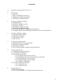
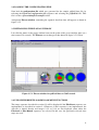
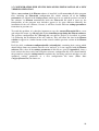
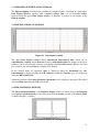
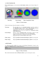
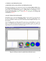
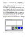
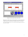
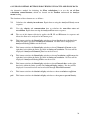
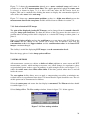
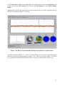
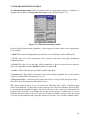
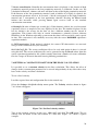
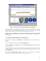
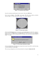
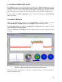
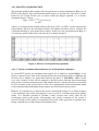
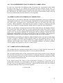
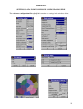
TOMOFLOW
FLOWAN USER GUIDE
Software version 1.33
Issue 2
May 2006
Tomoflow Ltd
86, Water Lane,
Wilmslow,
Cheshire.
SK9 5BB
United Kingdom
+44 1625 536672
[email protected]
CONTENTS
(i)
Summary of changes made since v1.21
1.
Introduction
1.1 Overview
1.2 The use of Matlab Scroll boxes
1.3 Software instruction conventions
1.4 The Flowan configuration file
2.
Setting up the Flowan software
2.1 Starting Flowan
2.2 Details of example data files
2.3 Loading a data file
2.4 Loading the configuration file
2.5 Initialising the Flowan window
2.6 Use of the File/Reset/Load/Reload menu functions
2.7 Configuration file status following installation of a new version of flowan
3.
Overview of Flowan window
3.1 The Data display window
3.2 The Statistics window
3.3 The Circular images
3.4 The text box
4.
Viewing concentration data
4.1 Identifying plotted concentration data
4.2 The basic screen functionality
4.3 Zooming the display
4.4 Use of control buttons to display concentration data
5.
Viewing velocity data
5.1 Calculating the golf ball velocity
5.2 Correlation considerations
5.3 Correlation tips and hints
5.3.1 Setting the time limits for analysis
5.3.2 Defining the flow direction and velocity convention
5.3.3 Determining the direction of flow
5.3.4 Setting the displayed speed limits
5.3.5 Additional information
5.4 Use of the velocity test data file
5.4.1. loading the data
5.4.2 analysing the data
6.
Viewing flow data
6.1 Flow rate calculation
6.2 Use of control buttons for viewing velocity and flow data
2
7.
Other important program options
7.1 Display parameters
7.1.1 Concentration scale
7.1.2 Gain of circular ect images
7.2 Zeroing options
7.3 The Reconstruction menu
7.4 Setting a constant Velocity for the flow calculation
7.5 Changing the sensitivity and zone maps
8.
Analysing particulate flows
8.1 Loading the data
8.2 Zeroing the captured data
8.3 Viewing the concentration data
8.4 calculating the velocity and flow data
8.5 Extended menu options (data display menu)
9.
Operation in batch mode
9.1 To analyse a set of capacitance data files
10.
FlowanRT
10.1 Introduction
10.2 Overview of software operation
10.3 Initialising Flowan
10.4 Initialising FlowanRT
10.5 Initialising ECT32
10.6 Setting the flowanRT display parameters
10.6.1 The flowanRT window
10.6.2 Setting up FlowanRT
10.7 Streaming the data
10.8 Interpretation of data
10.9 Further information about the FlowanRT window
10.10 To process another data file
10.11 Processing real-time data
Appendix 1
Measurement of velocity profiles in ECT systems
A1.1 Basic principle
A1.2 Practical realisation
A1.2.1 Velocity resolution enhancement by use of interpolation
techniques
A1.2.2 Effect of width of correlation window
A1.3 Appodisation
A1.4. Normalisation of correlation coefficients
A1.5 Use of differentiation to improve correlation
A1.6 Effect of flow patterns on correlation
A1.7 Correlation window size
A1.8. Calculation of flow
Appendix 2
Parameter settings in Refconfig.ini file
Appendix 3
Flowan parameter list
3
1 INTRODUCTION
1.1 OVERVIEW
Flowan is an off-line program which processes capacitance data captured using a twinplane ECT sensor and measurement system (such as the Tomoflow R100/PTL300E
equipment) to produce velocity and flow profiles and overall flow data for a mixture of 2
dielectric materials.
Flowan generates instantaneous concentration profiles of the flow inside the ECT sensor, at
two axial measurement locations (planes) for each frame of capacitance data. These
concentration profiles can be calculated for a relatively small number (typically 13) of userdefined zones in the flow cross-section. Cross-correlation techniques can then be used to
derive the instantaneous velocity in each zone from the concentration profiles at the 2
measurement planes. The overall flow profile can also be calculated from the concentration
and velocity profiles. The Flowan software displays very detailed informaton about the flow
structure in both numerical and graphical formats. A typical Flowan screen is shown in figure
1.1 below.
Figure 1.1 A Typical Flowan screenshot
Detailed information about the operation of the Flowan software is given in the Tomoflow
User Manual.
This additional Flowan User Guide is intended for new users of the Tomoflow R100 system
and demonstrates some of the most important aspects of the Flowan software by the use of
two example data files, which are supplied with the Flowan software.
The remaining paragraphs in this introductory section describe some background information
about the way the Flowan software operates and should be read carefully before attempting to
use the Flowan software for the first time.
4
1.2 USE OF MATLAB SCROLL BOXES
Flowan is a Matlab program and is controlled by a Windows-style user interface. However,
Matlab user interfaces operate slightly differently from standard Windows user interfaces,
particularly in the way options are selected in Matlab scroll boxes. This section describes
how to use Matlab scroll boxes.
Figure 1.2 A Matlab window containing a scroll box
The From box in figure 1.2 above is a scroll box. In a scrollbox, parameters are selected by
left-clicking the mouse on the up/down arrow buttons at the RH side of the scroll box. The
available options scroll up or down as black text on a light grey background.
When the required option appears, it is selected by left clicking inside the scroll box, when
its appearance changes to highlit grey text on a dark blue background. This is equivalent
to clicking an "OK" or similar button in a Windows interface to confirm the parameter
selection.
Note that it is not sufficient to merely scroll to the required option, it must be selected as
described above, otherwise the previously selected (or default) option will remain in effect.
1.3 SOFTWARE INSTRUCTION CONVENTIONS
The Flowan user interface window contains a combination of menus and control buttons.
In this Flowan User Guide, we describe menu use in terms of sequences in "shorthand"
format, such as:
File>Load>filename.
This means:
Left click on the File menu in the Windows menu bar (a drop-down menu appears)
Left click on Load in the drop-down menu.
Select the required Filename (after locating the appropriate folder if necessary)
1.4 THE FLOWAN CONFIGURATION (.INI) FILE
When Flowan starts up, it loads a special default Configuration file (Flowan.ini). This file
contains software control parameters which are defined by the user in the Flowan Settings
menu. These settings parameters are automatically saved to this special file each time the
Flowan program is exited. As the data in this file is overwritten each time the Flowan
program is run, it is a good idea to save an additional custom configuration file with a
unique file name, each time the program is run for a new set of input data. This ensures
that the data can be re-processed using the optimum parameter set.
5
2. SETTING UP THE FLOWAN SOFTWARE
2.1 STARTING FLOWAN
Open the ECT program group window by double-clicking on the ECT program group
icon on the PC desktop. Then double click on the Flowan icon in the ECT program group
window. The startup Flowan window, similar to the one shown in figure 2.1 below, will
appear.
Figure 2.1 Blank Flowan window
The top window is shown blank in figure 2.1 above, but in practice may display some
experimental data if a data file was loaded during previous use of the software.
Select File>Reset to clear any previously-loaded data. The Flowan window should now
revert to that shown in figure 2.1.
2.2 DETAILS OF EXAMPLE DATA FILES
The operation of the Flowan software will be demonstrated initially, using a set of test data
generated by dropping a thin-walled plastic ball of OD 50mm, filled with polypropylene
beads, down a vertical plastic tube of OD 60mm and ID 53mm. An 8-electrode twin-plane
ECT sensor, with a spacing between the measurement planes of 13cm, was located on the
outside of the tube and a Tomoflow R100 measurement system, operating at a rate of 200
frames per second (fps) was used to capture data over a 10 second period, during which the
ball was dropped down the tube. The ECT sensor was calibrated using air and densely-packed
polypropylene beads. The file name of the sample data file containing this captured data is
golf ball.bcp.
6
2.3 LOADING A DATA FILE
Load the captured twin-plane ECT data file golfball.bcp using the File>Load sequence. This
opens a select file to open window as shown in figure 2.3.1 below.
Figure 2.3.1 Select file to open window
Select the required file which is in the c:\Flowan\Datafiles\Examples folder. The Flowan
Zone and Pixel Chooser window appears, as shown in figure 2.3.2 below.
Figure 2.3.2 Zone and Pixel Chooser window
Click on the load Zone (map) button. The Select Zone (map) file window (as shown in
figure 2.3.3 below) appears.
Figure 2.3.3 Select Zone File window
7
The Zonemaps folder contains a number of preset zone-maps for 8 and 12-electrode
sensors. For example, zonemap8_4 is a 4-zone map for an 8-electrode sensor.
Select zonemap8_13 and click the Open button. The 13-zone map shown in figure 2.3.4
below appears in an updated Zone and Pixel chooser window.
Figure 2.3.4 Updated Zone and Pixel chooser window
Click the Finish button to accept this zone map. The loaded data will appear in the upper
Data Display window, which will appear similar to that shown in figure 2.3. below.
Figure 2.3.5 Flowan window with loaded golf ball data
8
2.4 LOADING THE CONFIGURATION FILE
Now load the configuration file which was generated for the sample golfball data file, by
selecting the File>Load configuration file sequence and selecting the golfball.ini file. This
file is in the c:\flowan\datafiles\examples folder.
An updated Flowan window, containing the captured data flow data will appear as shown in
figure 2.3.5.
2.5 INITIALISING THE FLOWAN WINDOW
Left click the mouse in the upper window between the peaks of the green and blue plots (at a
time around 5.9 seconds). The Flowan screen changes to that shown in figure 2.5.1 below.
Figure 2.5.1 Flowan window for golf ball data at 5.905 seconds
2.6 USE OF FILE/RESET/LOAD/RELOAD MENU FUNCTIONS
The image sequence described in section 2.3 will be displayed if the File>Reset sequence was
implemented as described in section 2.1. However, if this sequence is not implemented, the
data file is loaded directly and images 2.3.2 to 2.3.4 are not displayed when either the
File>load or File>Reload sequences are selected. In this case, the previously-selected zone
maps are used.
9
2.7 CONFIGURATION FILE STATUS FOLLOWING INSTALLATION OF A NEW
VERSION OF FLOWAN
When a new version of the Flowan software is installed, it will over-write all of the program
files, including the Flowan.ini configuration file, which contains all of the settings
parameters (as defined in the Settings menu) which were in use with the previous version of
the software. As Flowan automatically loads the Flowan.ini file when it starts up, the
functionality of the program may therefore appear to be quite different following the
installation of the new software, because it will have loaded different settings parameters
from those in previous use.
To avoid this problem, it is therefore important to save the current Flowan.ini file to a new
and unique file name (eg oldconfig.ini) before installing or updating the Flowan software.
The previous configuration file (oldconfig.ini) can then be loaded (as described in section
2.4) following the installation of the new software. This will allow the data in the Flowan
window to appear in a similar format to that viewed with the previous version of the Flowan
software.
If all else fails, a reference configuration file (refconfig.ini), containing basic setings which
should allow almost any normal data file to be analysed, is is now supplied with the Flowan
software. The values of the settings parameters in this file are given in Appendix 2. Once a
basic analysis has been caried out using this reference configuration file, users should modify
the parameters using the settings menu to optimise the data being analysed and then save the
optimised settings parameters to a new configuration file name (File> Save
confige>filename.ini) for future use.
10
3 OVERVIEW OF THE FLOWAN WINDOW
The Flowan window is divided into a number of component parts, consisting of a large upper
Data Display Window, together with a statistics window and a set of 4 circular images
located below the upper Data display window. A text box is located at the bottom of the
Flowan window.
3.1 THE DATA DISPLAY WINDOW
Figure 3.1 Data display window
The upper Data Display window shows zone-based, time-related data, which can be
concentration, velocity and/or flow rate. Data for individual frames for display in the lower
windows can be selected with a mouse or keyboard-controlled time cursor. When a new data
file is loaded, the data for Zone 1 is displayed by default.
In the normal mode of operation, time is displayed along the horizontal (x) axis,
concentration is displayed along the LH vertical (y) axis and Velocity (speed) is displayed
along the RH vertical axis.
Alternative options allow inter-electrode capacitances to be displayed along the LH vertical
axis and Flow rate along the RH vertical axis.
3.2 THE STATISTICS WINDOW
The lower left hand window is the Statistics display, which can show either a correlogram
or the power spectral density for the data centred on the frame selected at the cursor point,
as shown in figure 3.2 below.
Figure 3.2 Statistics display in correlogram mode
11
3.3 CIRCULAR IMAGES
Four circular images are located under the data display window and are shown in figure 3.3
below.
Zone Map
Derived image
Plane 2 image Plane 1 image
Figure 3.3 Circular images
Details of the images (from left to right) are as follows:
Zone map:
The zone map shows the electrode locations around the outside of
the capacitance sensor, together with the zone locations inside the
sensor. Data for individual zones (or the inter-electrode
capacitances) can be selected and displayed by clicking the mouse
on the required zone.
Derived image:
Displays selected zone-based data (concentration, velocity or flow
rate) over the time period displayed in the upper Data display
window. Note that image is displayed using a colour scale where
largest pixel value is red and smallest values as blue.
Plane 2 image:
Displays pixel-based concentration image for plane 2 at cursor point
Plane 1 image:
Displays pixel-based concentration image for plane 1 at cursor point
3.4 TEXT AREA
An additional text box window for messages and additional information is located at the
bottom of the Flowan window as shown in figure 3.4.
Figure 3.4 Flowan Text Box
More detailed information about the Flowan window is given in subsequent sections.
12
4. VIEWING CONCENTRATION DATA
4.1 IDENTIFICATION OF PLOTTED CONCENTRATION DATA
Following the loading of a new experimental data file, the top Data display window shows
the average concentration (expressed as a percentage of the zone when full, in the nominal
range 0-100%) for the selected zone (shown as a white section in the zone map) at each of
the two measurement planes as a function of time. The Green trace corresponds to the
average zone concentration at Plane 1 and the Red trace corresponds to the average zone
concentration at Plane 2.
4.2 BASIC WINDOW FUNCTIONALITY
Left click the mouse in the upper Data display window at a time around 5.9 seconds (between
the red and green peaks in the concentration plots. Note that the time cursor can be
incremented a frame at a time using the PC cursor keys (left and right arrow keys on the
PC keyboard).
Select the centre zone in the Zone map (LH circular image) by left clicking on it with the
mouse. The Flowan window should now resemble that shown in figure 4.2.1 below and
shows the passage of the golf ball through the two measurement planes of the ECT sensor
approximately 5.9 seconds after the start of data capture.
Figure 4.2.1 Flowan window for golf ball data (ball inside sensor)
13
Move the time cursor one frame at a time using the PC cursor keys and note how the
circular images at the two measurement planes change. The concentration plots and the
image sequences both show that the ball passes through measurement plane 1 first, and then
passes through measurement plane 2, that is, plane 1 of the sensor is the upper plane.
The figures above the plane 1 and plane 2 concentration images give the concentration
values for the selected centre zone (100% when the ball is present) and for the overall
sensor volume (around 60%) for each frame of data.
Adjust the time cursor location using the cursor keys until the ball image size is maximised
at one of the measurement planes (eg at 5.910 seconds). Now select different zones with the
mouse and notice how the measured concentration varies over the cross-section of the
sensor. It is a maximum at the centre of the sensor and reduces towards the edge of the
sensor because the diameter of the ball is less than that of the sensor. Note that the
concentration values are higher in the zones at the side of the tube nearest to electrodes 6
and 7, showing that the ball passed down this side of the tube.
Also note the correlogram, (statistics display) which shows a very strong peak (with an
amplitude of 97.7% of maximum) at a time delay of 0.055 seconds and a frame delay of 11
frames. (As the time for each image frame at 200 fps is 0.05S, a figure of 0,055S corresponds
to 11 frames). Moreover, as the spacing between the sensor planes is 13cm, thevelocity can be
calculated approximately as 236.4 cm/S. A more accurate value, calculated from the
correlogram peak is 237.2 cm/S, as shown in the correlogram.
Now left click the mouse in the top window, well away from the time for which the ball is
inside the sensor (eg around 3 seconds). The new Flowan screen display is shown in figure
4.2.2 below.
Figure 4.2.2 Flowan window for golf ball data (ball outside sensor measurement planes)
14
Note that the two circular ECT images are now showing 0% concentration, as the sensor is
empty and also note that the correlogram is now showing no correlation peak, as there are
no concentration signals present (other than measurement noise).
4.3 ZOOMING THE DISPLAY
As the only area of real interest is the time perod for which the ball is inside the sensor, we
can examine this time interval in more detail using the zoom controls. We will use these tools
to examine the measured data between the new time limits of 5.5 and 6.5 seconds, as follows:
Left click the mouse on at a point approximately 5.5 seconds in the upper Data display
window, Right click the mouse and select start point.
Left click the mouse on at a point approximately 6.5 seconds in the upper window, Right
click the mouse and select end point.
Right click the mouse again and select the Zoom option. The screen display will change to
that shown in figure 4.3.1 below.
Figure 4.3.1 Flowan window for golf ball data (ball inside sensor, display zoomed)
The passage of the ball through the sensor can now be seen much more clearly, as the green
and red concentration plots show.
Note that the display can be unzoomed by right-clicking on the upper window and
selecting Zoomout.
15
4.4 USE OF CONTROL BUTTONS TO DISPLAY CONCENTRATION DATA
As an alternative to the use of the menus, much of the program functionality can be
controlled using the buttons located on the Toolbar located underneath the menu bar. The
buttons which control the display of concentration data are listed below:
Nw
The New button has the same effect as using the File>Reset menu sequence, which
removes all of the loaded data from memory. It is not necessary to use this
button before loading new data if the previously selected zonemap is to be re-used.
Ld
The Load button has the same effect as using the File>Load menu sequence,
rL
The Reload button reloads data for the previously loaded data file. It allows the
original data to be reloaded, without having to reselect the zone map, if the current
data file has been modified.
Zr
This applies a correction for zero drift in a similar manner to that implemented by
the Settings>zero menu sequence. The parameters used are those defined in the Zero
Settings data window. See section 7.2 for additional information.
St
This button defines the current cursor position on the Data display window to be
the start point of the zoom settings. This function may also be implemented using
Settings>Display>Zoom position or from Start point on the context sensitive
menu obtained by right-clicking on the Data display. The start time cursor is
displayed as a vertical green dotted line.
En
This button defines the current cursor position on the Data display window to be
the end point of the zoom settings. This function may also be implemented using
Settings>Display>Zoom position or from End point on the context sensitive menu
obtained by right-clicking on the Data display. The end time cursor is displayed as
a vertical red dotted line.
ful
This button shows the full (unzoomed) data set in the Data display window. This
function may also be implemented using Zoomout on the context sensitive menu,
obtained by right-clicking on the Data display.
Mk
This button shows the zoomed data set in the Data display window. This function
may also be implemented using Zoom on the context sensitive menu, obtained by
right-clicking on the Data display.
<
This button reverts to the previous zoom position on the Data display window set
through the use of the ful or Mk buttons.
>
This button reverts to the next zoom position on the Data display window set
through<.
The operation of the remaining control buttons is given in section 6.2 and further more
detailed information about the functions of all of the control buttons is given in the
Tomoflow User Manual.
16
5. VIEWING VELOCITY DATA
The principle of the method used in the Flowan to calculate velocity and flow data is
described in detail in Appendix 1, which contains detailed information about the choice of
parameters used to calculate the flow velocities.
5.1 CALCULATING THE GOLF BALL VELOCITY
The velocity of the ball can be calculated by correlating the concentration images on a
zone-by-zone basis between the two measurement planes. This is carried out as follows:
Click the LH mouse cursor between the two concentration peaks (at a time around 5.88
seconds).
Select Analyse>Velocity field. The average velocity in each zone will be calculated and the
velocity of the ball in the selected zone will be displayed as a blue line, as shown in figure
5.1 below.
Figure 5.1 Zoomed Flowan screen showing velocity plot for centre zone
In this case, the velocity in the selected centre (white) zone is constant, with a value around
240 cm/sec. The velocity in other zones can be displayed by clicking on the required zone in
the zone map. In this case, as there is a single object, all of the zone velocities are similar.
Note that the velocities in each zone for each frame of data are stored in a temporary file so
that they can be displayed as required and also used in any calculations of flow or flow rate
(see section 6).
17
5.2 CORRELATION CONSIDERATIONS
It is important to understand that the velocity can only be calculated if there is correlatable
data present. This can be demonstrated by un-zooming the upper window display (right
click and select Zoomout), where the results are shown in figure 5.2.1 below.
Figure 5.2.1 Unzoomed Flowan screen showing velocity plot
In this case, the blue velocity plot only exists for a short time period during the passage of
the ball through the sensor measurement planes. Outside this period, there is no
correlatable data. The period for which the velocity plot exists, depends to a large extent on
the width of the correlation window selected.
Further detailed information about correlation techniques can be found in Appendix 1.
18
5.3 CORRELATION TIPS AND HINTS
When the Analyse menu is used to generate velocity and flow rate data, the correlation
calculation is carried out using the parameters defined in the correlation settings window
shown in figure 5.3.1 below. This window is diplayed using the Settings>correlation menu
sequence.
Figure 5.3.1 Correlation settings window
5.3.1 SETTING THE TIME LIMITS FOR ANALYSIS
All of the frames in the loaded .bcp data file are analysed to produce the velocity and flow
data unless the Correlate zoomed only box in the correlation settings window is ticked. In
this case, only the data between the start and end points of the zoomed data is used for the
correlation calculations.
5.3.2 DEFINING THE FLOW DIRECTION AND VELOCITY CONVENTION
If the Plane 1 leads box is checked, the velocity is defined to be positive if the flow is from
plane 1 to plane 2 and negative if the flow is from plane 2 to plane 1.
If the box is unticked, flow from plane 2 to plane 1 is considered positive.
5.3.3 DETERMINING THE DIRECTION OF FLOW
Once the flow direction convention has been set defined as described in section 5.3.2 above,
the actual flow direction at any point in time can be easily determined by clicking the mouse
pointer in the concentration display and observing the correlogram. If the correlogram
peak is to the right of the central axis, the velocity is positive and if it is to the left of the
central axis, it is negative.
19
5.3.4 SETTING THE DISPLAYED SPEED LIMITS
The two numbers entered in the Speed limits boxes in the correlation settings window set the
lower and upper limits of the right hand velocity scale in the data display window. Sensible
speed limits should be set, otherwise spurious velocities may be generated that have no
physical meaning, and the analysis process may take an un-necessarily long time.
The correlation process will find positive and negative values of time delay and hence
velocity. If the direction of flow is unknown it is safest to set symmetrical positive and
negative speed limits initially, to ensure that the velocity plot is visible. Otherwise, for
example, if the speed scale is set to be only positive and the actual velocities are negative, no
velocity trace will be displayed.
5.3.5 ADDITIONAL INFORMATION
More detailed information about all of the correlation settings parameters can be found in
section 8.9 of the Tomoflow User Manual.
5.4 USE OF THE VELOCITY TEST DATA FILE
A pair of test files have been included in the Examples folder which allow the operation of
the velocity calculation in Flowan to be checked. The first file, (veltest.bcp) contains 2
seconds of forward flow at 50% concentration and two seconds of reverse flow, also at at
50% concentration, with a net flow of zero. The secondfile (veltest.ini) contains the
initialisation data for the velocity test file.
5.4.1. LOADING THE DATA
Use File>Load and elect the veltest.bcp data file, which is
c:\Flowan\Datafiles\examples folder. Click the Open button to load this data file.
in
the
Use File>Load config to load the veltest.ini configuration file, which is in the
c:\Flowan\Datafiles\examples folder.
5.4.2 ANALYSING THE DATA
Click on the All button to analyse the test data.
Select the centre zone in the Flowan window, which should now appear as shown in figure
5.4.1
20
Figure 5.4.1 Flowan window showing velocity testdata
The two sets of 2 seconds of data are shown commencing at t=2 and t=6 seconds for the
forward and reverse flows respectively. The velocity is constant during both periods at
+1000cm/S during the forward flow period and -1000cm/S during the reverse flow period.
The text box shows that the net flow is zero, made up from equal and opposite f positive and
negative flows of 990cm3.
21
6. VIEWING FLOW DATA
Once the velocity profiles have been calculated for each zone, it is possible to calculate the
flow profiles and overall flow rate for each frame of data.
6.1 FLOW RATE CALCULATION
The flow calculations are carried out by multiplying the average concentration and velocity
values in each zone and then multiplying this figure by the zone area, which gives the
instantaneous flow rate in each zone. These individual zone flow rates are then summated
over the pipe cross-section for each frame of data to give the average flow rate per frame.
These average frame flow rates are then summated over all of the frames of captured data to
give the overall flow.
It should be noted that these calculations give the volumetric flow rates and overall
volumetric flow. These figures can be converted into mass flow rates if the density of the
material is known and entered in the Settings>Correlations>Density box. The configuration
file golfball.ini contains the correct value of density (0.57) for the golf ball.
To calculate the flow rates, select Analyse>Flow.
The calculation is carried out for all of the zones in the zone map and all of the frames of
data and the results are displayed immediately in the text box as an overall volumetric and
mass flow in cm3 or g, assuming that a material density value has been entered in the
settings>correlation menu.
The flow rates in the individual zones can be displayed via the Settings>Display menu by
setting the Plot scroll box to Flow Rate. The flow rates are shown as a violet plot as shown in
figure 6.1.1 below.
Figure 6.1.1 Flow rate plot for central zone
22
*** Note that in this modse of operation, the Flowan software shows the overall frame flow
rate, irrespective of which zone is selected. ***
The overall flow reported in the text box in figure 6.1 is 57cm3, or 33g, which aproximates to
the nominal volume and mass of the golf ball used in the experiment (63 cm3/36g).
However, it is possible to increase the accuracy of the flow rate calculation by correcting for
any zero offset areas in the concentration calculation. The effect of this can be seen by
clicking on the All button, when the flow data is recalculated and the new data appears as
shown in figure 6.1.2 below.
Figure 6.1.2 Corrected flow data
The reported flow in the text box is now the correct value (63 cm3 and 36g ). Further
information about the use of the zero correction option is given in section 7.2.
Note that the flow rate plot exists for a wider time period than that for the actual physical
flow. This is a function of the width of the correlation window used for the calculation and
illustrates the averaging which occurs in the velocity/flow calculations. The use of a narrow
correlation window will reduce this effect and allow more rapid changes in velocity to be
viewed, although it will also result in poorer correlation. The use of a wider correlation
window will give a much slower response to velocity changes but with improved
correlation quality.
23
6.2 USE OF CONTROL BUTTONS FOR VIEWING VELOCITY AND FLOW DATA
An alternative method for initiating the Flow calculations is to use the set of flow
calculation control buttons, which are located on the Toolbar underneath the Analyse
menu heading.
The functions of these buttons are as follows:
Vl
Calculates the velocity in each zone. Equivalent to using the Analyse>Velocity menu
sequence.
Fl
Uses the velocity and concentration data to calculate the zone flow rates and
overall flow. Equivalent to using the Analyse>Flow menu sequence.
All
The use of this button effectively applies the Zl, Vl and Fl buttons in sequence and
allows the flow to be analysed in one button press.
Sp
This button switches the Data display window to show Speed on the right hand axis
within the limits specified in Settings>Correlation. No data will be displayed if
Analyse>Velocity field has not been used.
Fr
This button switches the Data display window to show Volumetric flowrate on the
right hand axis within the limits specified in Settings>Correlation. No data will be
displayed if Analyse>Volumetric flow has not been used.
Cp
This button switches the Data display window to show Correlation coefficient on the
right hand axis within the limits specified in Settings>Correlation. No data will be
displayed if Analyse>Velocity field has not been used.
Ex
This button switches the Data display window to show External data on the right
hand axis within the limits specified in Settings>Display settings. No data will be
displayed if external data has not been loaded through File>Load external.
Cr
This button switches the Statistics display window to show correlation coefficient
psd
This button switches the Statistics display window to show power spectral density.
24
7. OTHER IMPORTANT PROGRAM OPTIONS
A full listing of the functionalitity of the Flowan menu options is given in the Tomoflow
User Manual. The use of the some of the more important menu options in the Settings menu
will be discussed briefly in this section.
7.1 DISPLAY PARAMETERS
7.1.1 Concentration scale
The range of concentration values displayed in the upper display can be set using the
Settings>display>concentration plot limit boxes. To show the effect of changing these
values, select File>display>Concentration plot limits and input the values -0.1 and 0.1 into
the limit boxes as shown in figure 7.1.1 below.
Figure 7.1.1 Display settings sub-menu
Click on OK and a the screen will be updated. Now click on the rL button to re-load the
experimental data and select the centre zone. The modified Flowan window is shown below:
Figure 7.1.2 Flowan window using modified concentration scale
25
Figure 7.1.2 shows the concentration plotted over a more restricted range and it now is
possible to see the ECT measurement noise. This applies particularly when the centre zone
is selected, as shown in figure 7.1.2, as this is the zone where the ECT noise levels are
highest. This can be confirmed by clicking the mouse to display the concentration signals in
some of the other zones in the zone map.
Figure 7.1.2 shows up a measurement problem, as there is a slight zero offset between the
measurement data for the two planes and this will be discussed further in section 7.2.
7.1.2 Gain of circular ECT images
The gain of the displayed circular ECT images can be changed from its normal value of 1
using the image gain scroll box. To show the effects of this, first move the time cursor to a
position where an image of the ball is displayed as a circular ECT image at either plane 1 or
plane 2.
Now select Settings>display and use the scroll box to set a new image gain of 5. Click on the
OK button and the change in the circular ECT image will be obvious. Note that the
concentration scale in the upper window and the concentration values in the lower ECT
images remain unchanged.
Ths facility is useful for displaying ECT images at weak concentration levels.
Reset the image gain to 1 in the image gain scroll box.
7.2 ZERO OPTIONS
All measurement systems are subject to drift and offset problems to some extent and ECT
measurement systems, which attempt to measure very small changes in capacitance values
are particularly prone to these types of problem. A good example can be seen in figure 7.1.2,
where the centre zone shows finite offset shifts in the time periods where there is no ball
inside the sensor.
The zero option facility allows users to apply a compensating zero offset to minimise any
residual offsets in experimental data where it is known that the signal should be zero. The use
of this option can be demonstrated as follows:
Select the centre zone and ensure the data display is unzoomed. The Flowan window should
ressemble figure 7.1.2.
Select Settings>Zero. The Zero settings window, shown in figure 7.2.1 below appears.
Figure 7.2.1 Zero settings window
26
Set the From box to start, set the start (time) box to 0 (seconds) and set the Length box to 4
seconds. Click on the Zero button, then Click on the Close button to exit the Zero settings
menu.
All of the data will be auto-zeroed, based on the data in the first 5 seconds of the data file and
the efects are shown in figure 7.2.2 below.
Figure 7.2.2 Flowan screen following zeroing based on first 5 seconds of data.
Comparison between figures 7.1.2 and 7.2.2 shows that the sets of data for each measurement
plane are now fairly well-superimposed (figure 7.2.2), whereas previously (figure 7.1.2) there
was a positive vertical offset between the plane 1 data (green) and the plane 2 data (red).
27
7.3 THE RECONSTRUCTION MENU
The Reconstruction menu, which determines how the permittivity image is calculated, is
displayed by clicking on Settings>Reconstruction. and is shown in figure 7.3.1.
Figure 7.3.1 The Reconstruction window
Details of the Reconstruction parameters (with suggested default values where appropriate)
are as follows:
1. Model: The concentration/permittivity model to be used (Parallel, Series or Maxwell).
2. K: The ratio (>1) of the permittivity of the mixture at the lower and upper permittivity
calibration points.
3. Ksolid: The ratio (>1) of the bulk (solid) permittivity of the two materials in the mixture.
Note, for a liquid/gas mixture, Ksolid should be set equal to K.
4. Gain(1): The feedback gain used in the iteration algorithm
5. Iterations (0): The number of iterations used in the iteration algorithm. To set no iterations
(equates to simple LBP reconstruction) set = 0.
6. Image truncation: Calculated pixel values outside the set range will be truncated to have
the values set in the image truncation limits boxes.
This allows physical limits to be set to limit the allowable pixel values. Confining these
values between 0 and 1 is physically realistic, but may not always be optimum. Because ECT
is an approximate imaging technique, the pixel (and hence zone) values may fall outside the
nominal range of 0 and 1, even though the average for the image as a whole may be correct.
Limiting the pixel values to 0 and 1 may lose useful correlatable structure from the signal
cause the speed estimation to be degraded. Limits of -0.4 and 1.4 are sensible common values.
28
7. Invert normalisation: Normally the concentration data is displayed as the fraction of high
permittivity material present in the low permittivity material, as calibrated. In this case, the
calculation of flowrate, volumes and mass will then be that of the higher permittivity material.
If the flowrate of the low permittivity material (such as bubbles in a liquid) is required, the
concentration parameter needs to be inverted, s that 0 (corresponds to the high permittivity
material and 1 corresponds to the low permittivity material. Pressing the Invert button
initiates this inversion, while pressing Invert again reverses back to the standard
concentration convention.
8. Resample (In units of frames per second (fps)): If this button is clicked, the set of measured
capaciance data is re-sampled at the rate displayed in the box. The number displayed in the
box by default is the average for the data set, but a different number may be entered if
appropriate. This feature may help in certain circumstances, primarily because inherent
limitations in the Windows operating system mean that data is not necessarily evenly spaced
in time. This correction is not normally necessary with the newer DAM200E capacitance
acquisition module.
9. C/K Linearisation: If this option is checked, the sensor C/K charcteristics are corrected
using a sensor coefficients file (see 10 below).
10. Pick Coeff. file: The sensor coefficients file to be used with option 9 above is selected
using this box. The sensor coefficients file can be generated using the Recal softare from the
sensor capacitance/permittivity file, which contains data from a number of sensor calibration
files for a range of dielectric materials havving differing permittivities.
7.4 SETTING A CONSTANT VELOCITY FOR THE FLOW CALCULATION
It is possible to set a constant velocity for the flow calculation. This allows the effect of
changes in the reconstruction parameters to be viewed independently of any effects these may
have on the velocity and flow calculations.
To set a fixed velocity:
Load the required data and configuration files in the normal way.
Select the Settings> Set fixed velocity menu option. The Velocity window shown in figure
7.4.1 below will appear.
Figure 7.4.1 Set fixed velocity window
Type in the required velocity (in this case, 1000 cm/S) and click The OK button. The set
velocity will be shown in the data window as a blue line. Figure 7.4.2 shows a typical
example.
29
Figure 7.4.2 Data window showing constant velocity of 1000cm/S
To analyse the flow using this constant velocity, first click on the Zr button to zero any
residual offsets in the concentration plots (details in section 7.2) and then click on the Fl
button to analyse the flow, details of which will be displayed in the text area.
Note: Do not use the All button, as this will over-ride the constant velocity setting and will
calculate the flow by deriving the velocity from the concentration plots using correlation in
the normal way.
7.5 CHANGING THE SENSITIVITY AND ZONE MAPS
The method for changing the sensitivity and zone maps used for reconstruction, is as
follows:
1. Copy the required sensitivity map to the Flowan\smaps folder.
2. Select the Settings > Sens maps menu option. The Sensitivity maps window will appear as
shown in figure 7.5.1.
3. Type in the relative address of the new sensitivity map against the sensor type in use. In the
example in figure 7.5.1, the new map for an 8-electrode (28 meassurements) sensor has the
name Sintef8_32.sif
Note that in the measurements column in figure 7.5.1, 15 corresponds to a 6-electrode
sensor, 28 to an 8-electrode sensor and 66 to a 12-electrode sensor.
30
Figure 7.5.1 Sensitivity map window
Once the sensitivity map filename has been entered, click on the OK button.
Now select the Settings > Zone Maps menu option. The Zone maps window, previously
shown in figure 2.3.2 and repeated here as figure 7.5.2, will be displayed.
Figure 7.5.2 Zone maps window
Click on the Load zone button and select the required zone map as described in section 2.3.
Finally, click on the Finish button. The Zone map will be generated from the new sensitivity
map and the user is asked to confirm that the new map is to be used in the window shown in
figure 7..5.3 below.
Figure 7.5.3 Zone map confirmation window
Click on the Yes button. All further processing of the measured data will be carried out using
the new sensitivity and zone maps.
The new map configuration can be made permanent by saving the configuration file.
31
8. ANALYSING PARTICULATE FLOWS
The golfball data gives a good insight into the operation of the Flowan software but this data
is not typical of most practical flow regimes. In this section we will use a set of more realistic
flow data, captured by monitoring plastic beads falling vertically under gravity. The tube
and ECT sensor used to produce this data were identical to those used for the golf ball data.
In this section, the software operation will be demonstrated using the control buttons
wherever possible.
8.1 LOADING THE DATA
Click on the Ld button and select the gravityflow.bcp data file, which is in the
c:\Flowan\Datafiles\examples folder. Click the Open button to load this data file.
Use File>Load config to load the gravityflow.ini configuration file, which is in the
c:\Flowan\Datafiles\examples folder.
Select the centre zone in the Flowan window, which should now appear as shown in figure
8.1 below.
Figure 8.1 Flowan window for gravity flow of plastic beads
The window shows that the plastic beads flow for approximately 4 seconds during the 13
seconds of captured data.
32
8.2 ZEROING THE CAPTURED DATA
Figure 8.1 shows that there is a zero offset problem in the captured data and it is therefore
worth dealing with this problem before processing the data further.
Select Settings>Zero and set the menu to zero the first 6 seconds of data as shown in figure
8.2.1 below.
Figure 8.2.1 Zero settings window
Click on the Set Zero button and then close the window. The corrected Flowan window
shown below will appear. Select the centre zone.
Figure 8.2.2 Gravity flow data after zero correction
Note that the Plane 1 concentration data (green) is at a higher overall level than that for the
plane 2 (red) data. This is not a measurement error but is simply a result of lowered
concentration caused by the acceleration of the plastic beads under gravity between the two
measurement planes (which are separated by a distance of 13cm).
33
8.3 VIEWING THE CONCENTRATION DATA
Use the Zoom controls to display the main region of flow as follows:
Left click in the Data display window at a time around 6 seconds and then click the St (start
zoom) button.
Left click in the Data display window at a time around 11 seconds and then click on the En
(end zoom) button.
Finally click the mouse cursor in the centre of the flow data, at a time around 8.5 seconds.
The Flowan screen should now resemble that shown in figure 8.2.3 below:
Figure 8.2.3 Flow data with zoom points set.
Now click on the Mk (Zoom in) button. The screen changes to that shown in figure 8.2.4 and
shows the flow of beads on an expanded time scale.
34
8.2.4 Zoomed Data
8.4 CALCULATING THE VELOCITY AND FLOW DATA
From figure 8.2.4, it is clear (even from the apparently semi random concentration
measurements), that the data in Plane 1 (green) leads that in plane 2 (red).
In fact, the data is relatively well-correlated, as can be seen by clicking the mouse cursor in
the data at various time points and examining the correlogram for a range of zones.
Now click on the All button to analyse the data to produce the velocity and flow information.
The velocity in the centre zone will be displayed as shown in figure 8.2.5.
By clicking on the zone map to select a range of zones, explore how the particle velocity
changes over the tube cross-section. It is highest at the centre of the tube and reduces
towards the walls, as expected for this type of flow.
Note that the text box gives the overall flow of materials as 927 cm3.
35
Figure 8.2.5 Velocity plot for centre zone
8.5 EXTENDED MENU OPTIONS (Data Display menu)
If the right hand button of the mouse is clicked inside the main data window area, a further
menu apears as shown in figure 8.2.6.
Figure 8.2.6 Extended menu
This window has already been used (section 4.3) to zoom the display. It also contains a
number of useful plotting and export options, which are described fully in section 8.3 of the
Tomoflow User Manual.
36
9. OPERATION IN BATCH MODE
The Flowan software can be used to process one or more data files automatically in Batch
Mode, which is selected using the File menu.
The parameters used in the analysis will be those previously entered in the Settings menu.
Batch mode operates as follows:
9.1 TO ANALYSE A SET OF CAPACITANCE DATA FILES
The capacitance data files to be analysed must first be located in a single folder and the
parameters to be used in the analysis must be set in the Settings menu as for operation in
normal (single file) mode. Once this has been completed, the files can be analysed as follows:
Use the File > Batch Analysis menu sequence to open the Batch mode window shown in
figure 9.1.
Figure 9.1 Batch mode window in data selection mode
Click on the Choose file dir button and select the folder containing the data files to be
analysed. The file names will appear in the data area.
To analyse all of the data files, click on the Analyse all button. The data files will be
analysed and the results will appear in the data area of the window as shown in figure 9.2
Figure 9.2 Batch mode window in results mode
The results can be saved as a text file by clicking on the Save Text button and entering a
suitable file name. Note that the file name should contain the extension .txt.
The following points should be noted when using batch mode:
37
1. If the data files are large, the analysis will take a considerable time, typically many
minutes.
2. If a constant velocity is set, the Auto zero option in the batch window must not be
checked.
3. The results will be processed for a period of time nominally equal to that of the recording
period. However, some data will be missrd at the start and end of the file equal to the length
of the correlation window set in the correlation settings menu. So, if there is 10 seconds of
data and the correlation window is set to 1 second, only the middle 8 seconds of data will be
processed.
4. The batch analysis option can be used to measure the average concentration by entering a
fixed velocity for the data file (eg 100cm/S) and calculating the volumetric flow for this
velocity. It can then be compared with the maximum possible flow, which can be calculated
using the formaula Max flow = A * V* T , where A is the internal cross-sectional area of the
sensor in cm^2 , V is the set velocity (100 cm/S) and T is the period of the analysed data (=
measurement duration - 2* correlation window length) in seconds.
5. The remaining control buttons in the batch window allow individual (high-lighted) files to
be analysed [Analyse] or set to be the first file to be analysed in the list displayed in the
window [Analyse from here].
A typical set of output data is shown in figure 9.3.
Wheat_AH_m1_loose_full.bcp vol 28226cm^3 mass 28226g Ave Vel(cm/sec) Min 100(z1) Max 100(z1) Unacc. 0.0%
Wheat_AH_m2_loose_full.bcp vol 28230cm^3 mass 28230g Ave Vel(cm/sec) Min 100(z1) Max 100(z1) Unacc. 0.0%
Wheat_AOH_m1_loose_full.bcp vol 28225cm^3 mass 28225g Ave Vel(cm/sec) Min 100(z1) Max 100(z1) Unacc. 0.0%
Wheat_AOH_m2_loose_full.bcp vol 28239cm^3 mass 28239g Ave Vel(cm/sec) Min 100(z1) Max 100(z1) Unacc. 0.0%
Wheat_APW_m1_loose_full.bcp vol 28219cm^3 mass 28219g Ave Vel(cm/sec) Min 100(z1) Max 100(z1) Unacc. 0.0%
Wheat_APW_m2_loose_full.bcp vol 28221cm^3 mass 28221g Ave Vel(cm/sec) Min 100(z1) Max 100(z1) Unacc. 0.0%
Wheat_CH_m1_loose_full.bcp vol 28229cm^3 mass 28229g Ave Vel(cm/sec) Min 100(z1) Max 100(z1) Unacc. 0.0%
Wheat_CH_m2_loose_full.bcp vol 28222cm^3 mass 28222g Ave Vel(cm/sec) Min 100(z1) Max 100(z1) Unacc. 0.0%
Wheat_CH_m3_loose_full.bcp vol 28233cm^3 mass 28233g Ave Vel(cm/sec) Min 100(z1) Max 100(z1) Unacc. 0.0%
Wheat_FR_m1_loose_full.bcp vol 28228cm^3 mass 28228g Ave Vel(cm/sec) Min 100(z1) Max 100(z1) Unacc. 0.0%
Wheat_FR_m2_loose_full.bcp vol 28222cm^3 mass 28222g Ave Vel(cm/sec) Min 100(z1) Max 100(z1) Unacc. 0.0%
Wheat_FR_m3_loose_full.bcp vol 28223cm^3 mass 28223g Ave Vel(cm/sec) Min 100(z1) Max 100(z1) Unacc. 0.0%
Wheat_TR_m1_loose_full.bcp vol 28252cm^3 mass 28252g Ave Vel(cm/sec) Min 100(z1) Max 100(z1) Unacc. 0.0%
Wheat_TR_m2_loose_full.bcp vol 28228cm^3 mass 28228g Ave Vel(cm/sec) Min 100(z1) Max 100(z1) Unacc. 0.0%
Wheat_TR_m3_loose_full.bcp vol 28236cm^3 mass 28236g Ave Vel(cm/sec) Min 100(z1) Max 100(z1) Unacc. 0.0%
Figure 9.3 Typical set of output data in batch mode
For further information about the use of the Flowan software, please refer to the Tomoflow
User Manual.
38
10. FLOWAN RT
10.1 INTRODUCTION
FlowanRT (Flowan Real-Time) is an additional real-time component of the Flowan
software suite. It operates on data streamed from the ECT32 software and allows live or
captured ECT data to be processed and displayed in real-time. FlowanRT calculates
speed, flow rate and accumulated volumetric and mass flow online and enables the Tomoflow
R100 system to operate as a real-time flow meter. FlowanRT is supplied as experimental
software, as it is still under development at present.
FlowanRT uses the same algorithms as the standard batch mode Flowan software, but is a
separate application. In principle, the accuracy should be similar to that of the Flowan
software when run on a modern fast PC. However, as FlowanRT runs in real-time under the
MS Windows operating system, small errors may be introduced because of the way in
which the operating system software interacts with the FlowanRT software. This will
become apparent if FlowanRT is used repetitively to analyse the same set of streamed
captured data.
The FlowanRT software operates as follows:
The Flowan software is used initially to set up the operating and flow algorithm parameters,
which are saved automatically in the Flowan.ini configuration file. These parameters are then
read automatically into the FlowanRT program when it is started. The ECT32 software is
then configured to control the capacitance measurement system and then FlowanRT is
configured to display and process the streamed data data in the required format. Once all of
the software has been configured, ECT32 is set to stream live or captured capacitance data
and this is displayed simultaneously in both the ECT32 and FlowanRT windows.
10.2 OVERVIEW OF SOFTWARE OPERATION
FlowanRT can be used with either live or experimental data. It's operation will be described
initially using the example data files supplied with the Flowan software. FlowanRT requires
the ECT32 program to be running simultaneously with FlowanRT and it is therefore
necessary to adjust the PC display screen to show both the ECT32 and FlowanRT windows
simultaneously.
10.3 INITIALISING FLOWAN
Open the Flowan software (NOT FlowanRT) by clicking on the Flowan icon in the ECT
Software group window and load the gravityflow.ini configuration file, as described in
section 2.4. Then close the Flowan software. This will automatically save the settings in the
gravityflow.ini file to the Flowan.ini configuration file.
Note that to use FlowanRT with any other data file or live data, the correct sensitivity and
zone maps must be loaded when Flowan is initialised.
10.4 INITIALISING FLOWANRT
Start FlowanRT by clicking on the FlowanRT icon in the ECT Software group window.
39
Figure 10.4.1. The FlowanRT window
The FlowanRT window will appear as shown in figure 10.4.1 above and the Flowan.ini
configuration file will be loaded automatically. Now temporarily minimise the FlowanRT
window to the Windows Task Bar.
10.5 INITIALISING ECT32
Start ECT32 and set up the Configuration window as shown below. Select the example data
file gravityflow.bcp, which is in the Flowan/datafiles/examples folder and use the
ssm8_32.sif sensitivity map.
Figure 10.5.1 ECT32 Configuration window
40
Click on the Setup System button. The main ECT32 window will appear.
Check that the example data file data plays back correctly in ECT32 by selecting Playback
mode and replay the data using the forward play ( > ) button in the ECT32 Control Panel.
Set ECT32 to Idle mode by clicking on the Idle mode button in the ECT32 control panel.
Now adjust the ECT32 window so that it appears as shown in figure 10.5.2, with only the
upper circular images and the ECT Control Panel displayed. To do this, ensure that the
ECT window is in the Restore Down mode (single square only displayed in the top RH
corner of the window, next to the close (X) box). Use the mouse to drag the top section of the
ECT image window to reduce its height, so that it just includes the two ECT images. Then
move the image window upwards, so that the PC screen is similar to that shown below.
Figure 10.5.2. Adjusted ECT32 window
Note that the ECT32 Control Panel can only be moved if it is in Idle mode.
Maximise the FlowanRT window by clicking on it in the Windows Task bar.
Now adjust the size and position of the FlowanRT window so that it can be viewed
simultaneously with the ECT32 windows, as shown in figure 10.5.3.
41
Figure 10.5.3 Adjusted ECT32 and FlowanRT windows
In the FlowanRT window, note the FlowanRT listening port number displayed in the
connection status box (lower left hand box at bottom of FlowanRT window). This will
typically be 3001 unless other software has already claimed that port.
In the main ECT32 window, open the ECT32 network connection dialog window. (File>Remote data streaming). The Network Connection window shown below will appear.
Figure 10.5.4. Network connection window
In the Target Network Address box, enter the network address of the computer running
FlowanRT, followed by a colon and then the FlowanRT listening port number. For
example, in figure 10.5.4, the network address is 192.168.0.100 and the port number is
3001. Note that PCs supplied with PTL ECT systems are all set up to have this network
address.
42
Click the Connect button. The Network Connection window changes to show that the
connection has been established, as shown below.
Figure 10.5.5. Network connection window following connection
Click on the Finish button. The display reverts to that shown in figure x.
ECT32 is now connected to FlowanRT.
The next step is to configure the FlowanRT window to display the data to be streamed from
ECT32.
10.6 SETTING THE FLOWANRT DISPLAY PARAMETERS
10.6.1 THE FLOWANRT WINDOW
Figure 10.6.1 The FlowanRT window
The FlowanRT window contains a number of real time values, a time series plot of one or
more of these values and a status area, as shown in figure 10.6.1 above. More detailed
information about the FlowanRT window is given in section 10.9.
43
10.6.2 SETTING UP FLOWAN RT
In the FlowanRT window, Select (tick) the Holdup (Concentration) box and unselect all of
the remaining boxes.
Set the upper holdup limit to 10(%) (box at top right of window) and the lower limit to 0(%)
(box above Set button), by typing the required values into the upper and lower y scale limit
set boxes. Confim these values using the Set button. The FlowanRT window should be
similar to that shon below in figure 10.6.2.
Figure 10.6.2 FlowanRT window holdup settings
Now unselect the Holdup box and select the Ave Speed box.
Set the upper speed limit to 500(cm/S) and the lower limit to 0(cm/S) by typing the required
values into the upper and lower y scale limit set boxes. Confirm these values using the Set
button. The FlowanRT window should now ressemble that shown below in figure 10.6.3.
Figure 10.6.3. FlowanRT window Speed settings
44
Now re-select the Holdup box. The upper set box will be greyed out and the lower set box
now determines the horizontal axis display time in seconds. Enter 10 (S) into the lower limit
box and confirm this value using the Set button. The FlowanRT software is now set up to
receive streamed data.
10.7 STREAMING THE DATA
In the ECT32 Control Panel window, select Playback mode and then click on the forward
play button. Data will be streamed and displayed to the FlowanRT window as shown in
figure 10.7.1 below.
Figure 10.7.1. FlowanRT window showing streamed data.
10.8 INTERPRETATION OF DATA
In figure 10.7.1, the Red trace is the average Concentration (Holdup) per frame inside the
sensor and the Green trace is the average velocity (speed) per frame inside the sensor.
The figures for Holdup, Average speed and FlowRate are instantaneous values. If the
Holdup and flow are zero at the end of data streaming, these values will also be zero in the
Flowan RT window at the end of data streaming.
The volume and mass flow figures are the integrated flows over all of the data frames on a
rolling basis. The final figure reported is the total flow.
10.9 FURTHER INFORMATION ABOUT THE FLOWAN WINDOW
The time series plot can display a selectable number of the realtime values, which are
selected using the plot selection check boxes as described in section 10.6.2. The y axis limits
are also configurable, but only when a single plot is selected. The Set button (not enter) is
used to confirm the data for each setting.
A scroll bar is located underneath the plot and facilitates viewing of the data after streaming
has finished. Under the scrollbar, there are two numbers, which indicate the time at the left
and right extremes of the plot.
45
If the initzero box is checked, a zeroing operation is carried out every time FlowanRT
starts. This is similar to the zeroing operation in Flowan, but is always carried out for a fixed
period – (400 frames or 2 seconds @200fps), one window length after streaming commences.
This is a useful option for lean flow conditions as it removes calibration or drift errors which
would otherwise integrate into a flow error over the flow period. These errors can dominate
the flow figures for lean flow conditions.
The following points should also be noted:
1. The real-time figures are correct at the time displayed by the time axis upper limit. There
will always be a delay of one window length between the real time data and the input stream –
this is a natural consequence of the algorithm used in FlowanRT.
2. The units and displayed resolution (number of decimal points) can be set in Flowan using
the Settings>Display menu sequence.
3. Holdup is the concentration or volume ratio averaged over all of the zones.
4. The Average speed is calculated from data for zones with valid velocities only.
5. The Flowrate is calculated from data for zones with valid velocities only. If the flowrate
window (set in Flowan->Settings->Display) is greater than zero, a second figure in brackets
indicates a rolling average over this window.
6. Volume is the Volumetric flowrate, accumulated from the start of data streaming.
7. Mass is the Mass flowrate, accumulated from the start of streaming.
10.10 TO PROCESS ANOTHER DATA FILE
Set the ECT32 software to Idle mode. This will reset the ECT Control Panel playmarker to
the start of the currently-loaded data file.
To replay and process the existing loaded data file, set ECT32 to Playback mode and start
the data playback. FlowanRT will automatically reset and will process the new set of
streamed data.
Alternatively, load a new data file to ECT32. This new data file can then be streamed to
FlowanRT in a similar manner.
***NB. If attempts are made to play back the data file backwards, this will cause the
FlowanRT software to crash. You have been warned!***
10.11 PROCESSING REAL-TIME DATA
The procedure for processing live data from an ECT system is almost identical to that for
recorded data. The only difference is that the ECT software must be set to Capture mode
rather than to Playback mode to start the streaming of data. Additional information on the
use of the FlowanRT software can be found in section 9 of the Tomoflow User Manual.
46
APPENDIX 1
MEASUREMENT OF VELOCITY PROFILES IN ECT SYSTEMS
This appendix explains how flow velocity profiles are extracted from capacitance data which
has been captured using a twinplane ECT system.
A1.1 BASIC PRINCIPLE
Concentration profiles are measured at two imaging planes which are separated by a finite
distance L. Equivalent pixels or zones (groups of pixels) in each measurement plane are then
correlated between the two image planes using the correlation equation:
R(τ) = (1/T) T/2C1(t). C2(t+τ)dt
(1)
-T/2
where R(τ) is the correlation coefficient, τ is a time delay parameter, C1 is the pixel or zone
value in the concentration profile at plane 1, C2 is the concentration value of the equivalent
zone or pixel at plane 2, t is the time (seconds) at which the measurements are made and and
T is the integration period (correlation window) in seconds.
Figure 1 shows the correlation coefficient (R) plotted against against time delay τ for one
zone of a typical set of ECT data. This graph is known as a correlogram and has a peak at the
time delay value τ which corresponds to the distance L between the image planes divided by
the flow velocity V. That is, at τ = L/V, which is known as the "flow structure transit time".
Note that as the integral is a continuous function, the correlogram is a continuous curve. If the
concentration profile images were identical in the two planes, the measurement system was
noise-free and the correlation window was infinite, the correlogram would have a normalised
value of 1 at this value of time delay and zero values everywhere else. However, for any real
system, the correlogram will have a peak coefficient less than 1, depending on the degree of
dispersion of the fluid flow, and finite, but lower values at other values of τ, as shown in
figure 1.
Figure 1. Sample correlogram
47
A1.2 PRACTICAL REALISATION
The principle outlined above implies that measurements are made continuously. However, an
ECT system captures data (concentration profile images) at specific time slots and at a finite
frame rate per second. In this case, we must rewrite the integral equation 1 as a discrete
summation process. That is:
R(p) = (1/N) Σ n=N/2 C1(n). C2(n+ p)
(2)
n=-N/2
where p is an integer frame number offset in the range (-N/2 < n <N/2), n is the measurement
frame number and N is the correlation window (the number of frames used to calculate the
correlation factor R(p) at the frame offset value p). In this case, the correlation factor R(p) is a
set of discrete points, plotted for each value of p, as shown in figure 2.
Figure 2. Discrete correlogram from equation 1
A1.2.1 Velocity resolution enhancement by use of interpolation techniques
In current ECT systems, the maximum data capture rate is limited to around 200fpS, ie one
frame is captured every 5mS. If the spacing between the measurement planes is 200 mm and
the flow rate is 10m/sec, the transit time between the planes is 200/10000 = 20mS. In this
case, only 4 frames of data will be captured as the flow moves from the first measurement
plane to the second measurement plane. This implies that the velocity will only be resolvable
to 25% accuracy at this speed because of the severe quantisation of the measurement which
results from the limited maximum frame capture rate of the measurement system.
However, if a smooth curve is fitted to the discrete correlogram of figure 2, as shown in figure
3, the maximum value of the correlogram is seen to occur at a location between the plotted
points. It is therefore possible to estimate a more accurate time delay value for the
correlogram peak by this means. Consequently, the velocity resolution of the system is
increased because of the ability to interpolate between the values generated by equation 2 by
fitting a smooth curve to the measured correlation values.
48
Figure 3 Continuous correlogram generated by curve fitting
A1.2.2 Effect Of Width of Correlation Window
The width of the correlation window determines the time constant of the velocity
measurement and the quality of the correlation. The correlation window must be always be
larger than the transit time of the flow between the 2 measurement planes (but see note A1.6).
If the two sets of measurements are poorly-correlated (ie the correlated/uncorrelated signal
ratio is low) then increasing the width of the correlation window will improve the amplitude
of the correlation peak in the correlogram. An example is shown in figure 4 below for the
same data processed with a narrow correlation window (red) and a wider window (blue).
Figure 4. Effect of changing width of correlation window
The wider correlation window improves the amplitude of the correlation peak relative to the
rest of the correlogram values but also increases the measurement time constant, reducing the
ability to see rapid changes in velocity.
49
A1.3 APODISATION
It is well-known that the use of a correlation window of finite width can cause problems if
there are major changes in the data sets to be correlated near the ends of the correlation
window. A typical example would occur when a slug is artificially truncated in one of the two
time variant functions by the correlation window. In this case, the truncated edge in one
function would be incorrectly correlated against the real edge in the other function.
To overcome this problem, the data within the correlation window is normally weighted to
give more prominence to the data close to the centre of the window by tapering the data
smoothly down to zero at the edges of the sampled region (window). This weighting process
is known as apodisation and there are a number of weighting functions which are commonly
used for this purpose, including Cosine and Hanning. The weighting is applied to each of the
constituent concentration profiles C1(t) and C2(t) before they are correlated.
Apodisation suppresses spurious peaks which would otherwise be produced in the
correlogram. One of the effects of apodisation is that a somewhat wider window is needed to
get the same effective window length. It also removes artefacts such as the velocity apparently
increasing exponentially as it would otherwise do in the above example.
A1.4. NORMALISATION OF CORRELATION COEFFICIENTS
The correlation factor R(τ) is normalised so that its maximum value is 1 for perfect
correlation whatever the amplitudes of the time variant signals (functions).
As we need to introduce the concept of autocorrelation for this normalisation process, we will
modify the terminology used so far to avoid confusion. The correlation coefficient between 2
different functions 1 and 2 will be written as R12, whereas the correlation coefficient between
2 identical functions (autocorrelation) will be written as R11.
The autocorrelation coefficient R11(τ) of C1(t) is defined as follows:
R11 (τ) = (1/T) T/2C1(t). C1(t+τ)dt
-T/2
(3)
The normalised correlation coefficient R12norm(τ) is calculated using equattion 4.
R12norm(τ)=R12(τ) / [R11(0) R22(0)]1/2
(4)
where R12(τ) is the cross correlation coefficient of of C1(t) & C2(t) and R11(τ) & R22(τ) are the
autocorrelation coefficients of C1(t) & C2(t) respectively.
50
A1.5 USE OF DIFFERENTIATION TO IMPROVE CORRELATION
In some cases, particularly for horizontal slugs of material, the concentration values within
the body of the slug are very uniform and correlation becomes difficult. In this case, it is
preferable to first differentiate the measurement data with respect to time and then correlate
the differentiated data. Differentiation works well for sudden concentration changes between
two levels without much structure otherwise (as in slug flow).
A1.6 EFFECT OF FLOW PATTERNS ON CORRELATION
The time delay τ, is the time by which the second plane information is delayed to calculate the
correlogram. It forms the x-axis of correlograms and therefore has many possible values. The
time delay at the correlogram peak is conventionally taken to be the transit time of the flow
structure. This assumption is valid when the flow structure is 'frozen' or identical at the two
planes, but is otherwise an approximation, which is however good for most normal flows.
If there are two distinct velocities present in the flow pattern then the correlogram will have
two separate and valid peaks. However, in many practical flow regimes there will be a range
of flow velocities, and the velocity information will be blurred together, producing multiple
peaks in the correlogram. Although the correlogram will (in principle) contain all of the
information about multiple delay times and dispersion (range of velocities), this complicated
information is difficult to extract from the correlogram in this type of flow situation.
Peak-finding by curve-fitting (or simply by taking the highest peak) can lead to sudden jumps
in what is actually a smoothly varying situation, when one peak gradually increases at the
expense of another and at one point or another has a higher numerical value. In this type of
situation, peak location using a centre of area calculation technique can produce smoother
velocity profiles, but in practice seems less reliable overall.
A1.7 CORRELATION WINDOW SIZE
The condition that the correlation window must be always be larger than the transit time of
the flow between the 2 measurement planes is necessary but not sufficient.
The correlation window must be long enough for the largest flow structures to pass from the
first end of the first plane to the second end of the second plane. Because of the finite lengths
of the measurement electrodes, this time will be longer than the nominal spacing between the
centres of the measurement electrode.
If the length between the centres of the measurement electrodes is L and each set of
measurement electrodes is of axial length l, then for any approximately spherical feature of
the same scale as the pipe diameter D, the time t taken from first arrival at the first electrode
to departure from the second is given by the equation:
t = V/(L+2l+D)
(5)
51
In practice V/(L+2l+D) is about twice the nominal transit time, though it may be more
depending on the sensor geometry. Equation 5 assumes the largest flow structures are at the
pipe diameter, which is reasonable for many flows, but not necessarily so for coherent slug
flows.
Although apodisation itself does not widen the peak, a wider correlation window is normally
used when apodisation (which is almost always used) is applied and this will widen the
correlation peak. Apodisation is part of the need to have correlation windows much greater
than the transit delay (see below).
Using apodisation means that the minimum effective window width is doubled. So allowing
an increased window width of 2x for flow structures and 2x for apodisation means that the
minimum realistic correlation window width is 4x the nominal value. As typical flow patterns
are statistically variable, in practice even wider windows are found to be necessary (up to 20x
the transit time). However, this will clearly have an adverse effect on the ability to see
rapidly changing velocities. In general, the use of wider correlation windows averages out
variations in velocity whereas the use of shorter windows allows more velocity structure to be
seen. The optimum choice of window size depends ultimately on the application.
For the closest approximation to mathematical exactness, high resolution concentration
profiles (using zones containing only a few individual pixels and captured using a sensor with
short electrodes) should be used.
A1.8. CALCULATION OF FLOW
Once the velocity profile has been calculated, it is necessary to take the products of the
concentration and velocity profiles and integrate these across the pipe section to obtain the
total flow. The default flowan method is to take the average of the concentration in the same
zone in each of the two measurement planes and to multiply this average value by the velocity
in the same zone. Alternatively, the concentration in either plane can be used if there are
known problems with the absolute concentration values in the other plane.
52
APPENDIX 2
SETTINGS DATA IN REFCONFIG.INI CONFIGURATION FILE
The reference configuration file refconfi.ini contains the settings in the windows below.
53
APPENDIX 3
FLOWAN PARAMETER LIST
The following is a list of the parameters used in the Tomoflow User Manual
A
Ai
Cross-sectional area of flow.
cross sectional area of ith zone
Cmax maximum inter-electrode capacitance which can be measured by ECT system
Cmin minimum inter-electrode capacitance which can be measured by ECT system
C1
C2
concentration in zone (plane 1)
concentration in zone (plane 2)
D
Df
Ds
pipe diameter (normally = Ds)
flow diameter of sensor contents
internal diameter of sensor
E
en
number of measurement electrodes in each measurement plane
nth electrode segment
f
sampling frequency (frames per second)
fc
anti-aliasing filter frequency **
k
integer multiplier parameter to determine required minimum spacing Ls between
measurement planes.
K1
Effective average relative permittivity of sensor contents with sensor filled with
lower permittivity material
Effective average relative permittivity of sensor contents with sensor filled with
higher permittivity material
K2
Le
Lf
Lg
Lm
Ls
axial length of earthed electrode
axial length of flow structure
axial length of driven guard electrode
axial length of measurement electrode
axial separation distance between centres of sets of measurement electrodes
R
Correlation coefficient
q1
q2
Volumetric flow rate of lower permittivity component of 2-phase mixture.
Volumetric flow rate of higher permittivity component of 2-phase mixture.
Q
Flow volume
s
sampling interval ( = 1/f) seconds
S
separation between centres of measurement planes (= Ls)
54
t
time interval between succesive frames (= s)
T
Time period window for correlation calculation
t1
start of flow measurement period
t2
end of flow measurement period
transit time of flow structure between measurement planes
also time delay in correlation equation
V
flow velocity between measurement planes
Z1
Typical capacitance per unit length measured between adjacent electrodes for a
practical ECT sensor
Typical capacitance per unit length measured between opposite electrodes for a
practical ECT sensor
Z2
55
(i) LIST OF CHANGES SINCE V1.21
1. An error in version 1.21 caused negative velocities to be ignored. This problem has been
corrected in V1.30
2. An additional example data file has been generated to allow the velocity measurement
characteristics to be checked. This file (veltest.bcp) contains 2 seconds of forward flow at
50% concentration and two seconds of reverse flow, also at at 50% concentration, with a net
flow of zero. The use of this file is described in a new section (5.4).
3. The implementation of the Maxwell and Series concentration/permittivity corrections has
been improved in the Reconstruction Window. An additional permitivity parameter, Ksolid,
corresponding to the ratio of the bulk (or solid) permittivities of the two materials inside the
sensor must now be entered in addition to the existing figure (K) which is the ratio of the
permittivities of the mixture at the lower and upper permittivity calibration points. More
details of the use of the Reconstruction parameters window are given in section 7.3.
4. A new facility has been introduced to allow the sensor Capacitance/Permittivity (C/K)
characteristics to be linearised using a sensor coefficients file which contains data derived
from a number of sensor calibration files for materials having a range of permittivity values.
The use of this lineraisation process improves both the image and concentration measurement
accuracies and is again described in section 7.3.
5. A facility to impose a constant velocity on the flow calculation has been included in section
7.4. This option allows the effect of changes in the concentration calculation to be seen more
clearly.
6. The method for changing sensitivity and zone maps has been improved and is described in
section 7.5.
Changes from v1.30 to 1.31
Problems loading new sensitivity maps have been corrected.
Changes from v1.31 to v 1.33
Batch processing mode modified to allow constant velocity to be set and used in batch mode.
Note auto zero setting in batch mode. Allows calculation of overall concentration. But must
correct for correlation window length.
UG notes: Extra zone map for one zone
Inversion problems K inverts
Derived image problems, normalisation, etc.
Display of plotting
Flow is overall, not zone-based
Reverse play of ECT32 crashes Flowan.
56