1
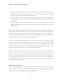
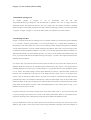
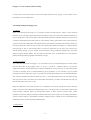
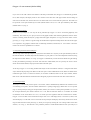
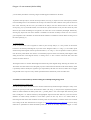
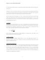
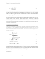
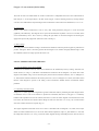
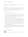
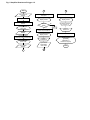
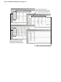
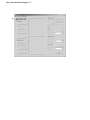
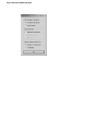
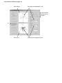
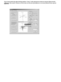
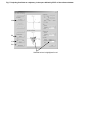
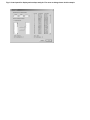
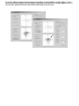
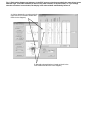
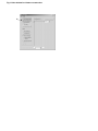
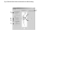
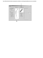
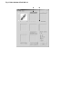
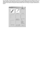
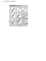
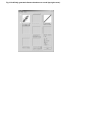
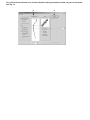
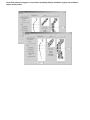
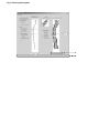
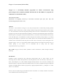
Polygon 1.5 user manual (18/Oct./2008) Polygon 1.5, a user-friendly Windows programme for climate reconstruction using palaeoecological data (seamlessly bundled with PolCalib 3.0 and PolHist 2.5: programs for calibration of reconstruction results). Takeshi NAKAGAWA Department of Geography, University of Newcastle, Newcastle upon Tyne, NE1 7RU, UK ([email protected]) Abstract This paper is a brief instruction of Polygon 1.5, the newly developed free PC software that principally performs quantitative climate reconstruction by modern analogue technique using palaeoecological datasets (pollen, diatom, etc.). The reconstruction can be done using either percentage values of all taxa or selected EOF axes. The program package also provides some other useful features including (i) visualisation of the distribution pattern of the reference dataset using 2-D or 3-D graphics of the space defined by EOFs, (ii) visualisation of the fossil dataset as the trajectory in the same EOF space, (iii) identification of outliers among the fossil dataset (envelope analysis), (iv) drawing temporary pollen diagram, (v) generation of error models specific to the reconstruction method and datasets, (vi) calibration of the reconstruction results using the error model, and (vii) the ability to export result figures to the clipboard. Polygon 1.5 has a very user-friendly graphical interface that helps users adapt to the software easily. An installer package of the software can be downloaded free of charge from the website <http://dendro.naruto-u.ac.jp/~nakagawa/ >. Key words: Polygon, PolCalib, PolHist, quantitative climate reconstruction, modern analogues technique, Palynology. Introduction Quantitative climate reconstruction using multivariate palaeoecological data (i.e. pollen, diatom, etc.) has increasingly become common and important in the field of Quaternary science since the early to mid 1990’s (e.g. Guiot, 1990; Nakagawa et al., 2002). Modern analogues technique (MAT) is one of the most commonly used methods among tens of proposed reconstruction methods because of its relatively straightforward logical background and ability of handling datasets without any regression by applying simplified models (e.g. Nakagawa et al., 2006; Tarasov et al., Submitted). However, when one intends to apply the method to his/her fossil dataset, it is normally inevitable to encounter a series of difficulties due to the following reasons: -1- Polygon 1.5 user manual (18/Oct./2008) (1) Most of the existing computer programs were not user-friendly, and were virtually impossible to use by people other than the developers and their colleagues (an exception to this rule is C2 developed by Juggins (http://www.campus.ncl.ac.uk/staff/Stephen.Juggins/software.htm)); (2) Reference datasets (i.e. surface pollen datasets in the case of palynology) were exclusively possessed by limited community members, and were not readily accessible (though this is not really true, most researchers were under this impression); (3) Even if one managed to obtain a reference dataset and figure out how to operate the software, it remained difficult to understand instinctively what the software was actually doing, because the output was normally only in the text format. Polygon 1.5 was developed in an attempt to solve all these problems. A key effort was made to provide a graphical and user-friendly interface. The installer package also includes Japanese surface pollen dataset established by Gotanda et al. (2002). The algorithms (both for reconstruction and calibration) are basically similar to Nakagawa et al. (2002) unless otherwise stated in this paper. The software is not protected by copy right, and can be freely downloaded from our web site <http://dendro.naruto-u.ac.jp/~nakagawa/>. A key strength of the method proposed by Nakagawa et al. (2002) is that it provides a new technique of estimating error ranges to the reconstructed climatic indices. The specific PC programs for this calibration (PolCalib 3.0 and PolHist 2.5) are still available on the same website. However, they are seamlessly integrated in Polygon 1.5, and users can calibrate their reconstruction results using the same (or slightly improved) algorithms, nearly without feeling that some modules of the Polygon 1.5 were originally independent programs. Polygon 1.5 is already becoming the software of choice for many users across the world. However, the author has received a lot of requests from users to provide written instruction, which did not previously exist. The aim of this paper is to meet these requests and provide the first complete instruction of Polygon 1.5. Hereafter, the instructions will be written assuming that the user is reconstructing climate in Japan using fossil and surface pollen datasets, just for clarity. However, this choice is essentially arbitrary and precisely the same approach can be applied to any other region for any environmental parameter. 0. Framework of Polygon 1.5 Fig. 1 is a simplified flowchart, showing only the main stream of climate reconstruction and results calibration by Polygon 1.5. Almost all the steps are performed either automatically or by clicking a single button. Normally the next action that needs to be made is indicated by (usually) one highlighted button. -2- Polygon 1.5 user manual (18/Oct./2008) 1. Installation of Polygon 1.5 An installer package of Polygon 1.5 can be downloaded from the web page <http://dendro.naruto-u.ac.jp/~nakagawa/>. The download has no limitation and is free of charge. Extract the downloaded zip file and double-click SetUp.exe file. Next, simply follow the ordinary procedures of installing Windows software. If successfully installed you will find a shortcut to the Polygon software in your Start menu (Start > Programs > Polygon > Polygon 1.5). You do not need to restart your computer to activate the software. 2. Formatting data files Polygon 1.5 requires at least three (or preferably four, if you intend to calibrate your reconstruction results) datasheets, i.e. (i) a surface (=reference) pollen dataset, (ii) a fossil pollen dataset. (iii) a climate dataset estimated at (or interpolated to) each surface pollen site, and (iv) an error model for climate estimation/interpolation (one datasheet for each climatic parameter). As for the scientific meaning of those datasets, please refer to our previous paper on the reconstruction/calibration methods (Nakagawa et al., 2002). If you are doing pollen-based climate reconstruction in Japan using the Gotanda et al. (2002) datasets, the files (i), (iii), and (iv) are all included in the installer package. The file (ii) is your data, which must be formatted according to the Polygon 1.5 protocol. This chapter describes how the datasheets must be formatted. It is crucial to keep your pollen taxa names and surface pollen site names as well as their order consistent across all datasheets. Make sure that all cells out of the data field are blank (having invisible “space” is one typical mistake in formatting datasheets). The easiest way to avoid this mistake is to copy the data field into a new spreadsheet and save it in csv format. The installer package contains sample datasheets for reference. Check the format carefully and harmonise your own datasheets in the same way as the sample data files. Choice of taxa is not essential for the software. Users can include any number of taxa in any order, as far as they are consistent between surface and fossil pollen data files. There is no limitation for either the taxa or pollen site name lengths. Users can also include as many climatic parameters as they want, but again the site names and their order need to be consistent between the surface pollen dataset and the dataset of climatic values estimated/interpolated to each surface pollen site (Fig. 2). All datasheets must be saved in csv format. Polygon has a function to re-calculate percentage values for the surface pollen values; i.e. you do not necessarily need to type-in percentage values instead of raw counts to the surface pollen dataset. However, fossil dataset must be expressed in percentage values, taking the sum of all pollen taxa included in the datasheet as 100%. If you put additional lines at the top and the bottom of the fossil data series and input zero value for all taxa, the depths (or ages) of those “void” horizons will be used as the top and bottom of the range of time series diagrams. If -3- Polygon 1.5 user manual (18/Oct./2008) you insert such “void” horizon with zero values in the middle of the data series, Polygon 1.5 will consider it as the discontinuity of curves at that horizon. 3. Envelope analysis by Polygon 1.5 3.1. Outline Before reconstructing climate, Polygon 1.5 is required to perform “envelope analysis”, which is a newly proposed method to check if the surface pollen dataset has wide enough coverage to be used for the climate reconstruction of the given fossil dataset. The envelope analysis starts from standard principal component analysis (PCA) (also known as empirical orthogonal function (EOF) analysis) of the reference (surface) pollen dataset. This is then followed by projection of the fossil pollen dataset in the multi-dimension space defined by the EOFs of the reference dataset. If a fossil pollen spectrum is within the area covered by the surface pollen dataset, then Polygon 1.5 considers that the fossil spectrum is “safe” to infer climate indices. For the fossil spectra that are out of the area covered by the reference dataset, Polygon 1.5 gives warning for those horizons as being presumably inappropriate to reconstruct climates using the reference dataset. The only solution for the latter case is to include more sites in the reference dataset and enlarge both the geographical and climatic coverage. 3.2. Data pre-treatment Fig. 3 shows the main window of Polygon 1.5, as viewed when you have just started the program. Click the “Import reference data” button at the left-upper corner (“A” in Fig. 3), choose the “1_Reference_data.csv” file from the sample data collection. Another small window of data pre-treatment for PCA will open (Fig. 4). If the surface dataset is already in percentage values (or contains different types of parameters) it is not necessarily a rule to perform percentage conversion. In that case, however, you need to be sure that the percentage values are calculated taking the sum of all taxa included in the reference dataset as 100%, i.e. not the total pollen sum nor the AP (arboreal pollen) sum. If you do not want to use certain taxa for the climate reconstruction, you need to exclude those taxa from your reference dataset and create a new csv file. Minor taxa enhancement can be done by square root or logarithmic conversion by clicking the check box and radio buttons. You can also choose between two different types of PCA: one using variance-covariance matrix and the other using correlation coefficient matrix, by clicking radio buttons. In short, variance-covariance matrix reflects dominance of each taxon, whereas correlation coefficient matrix treats all taxa equally. For an ordinary pollen dataset, variance-covariance matrix is recommended. Correlation coefficient matrix is suitable for cases of multidisciplinary datasets that contains variables expressed in different units. 3.3. EOF analysis -4- Polygon 1.5 user manual (18/Oct./2008) If you click on the “OK” button at the bottom of the data pre-treatment form, Polygon 1.5 automatically performs PCA (=EOF analysis) and display results on two windows in the main form. The upper window shows loadings of each taxon to the EOF axes, whereas the lower one shows EOF scores of each reference pollen site. The results can be expressed in 2-D space defined by two EOFs (default: EOF-1 and 2) or in 3-D space defined by three EOFs (default: EOFs 1-3) (Fig. 5). 3.4. How to save results? Results of every analysis (i.e. not only the PCA) performed by Polygon 1.5 can be saved both graphically and numerically. The easiest way is to put your cursor on the graphic window and click the right button of mouse. If the window is showing results of analyses, a popup menu will appear and options of “Copy” and “Save matrix” will be given (Fig. 6). “Copy” means to copy the image into the Windows clipboard in bitmap format. This allows the figure to be exported to any graphical software such as Photoshop, Illustrator, PowerPoint, etc. “Save matrix” allows the results to be saved in a spreadsheet in csv format. 3.5. Projecting fossil data in the EOF space The next step of the envelope analysis is to project the fossil dataset as a trajectory in the space defined by EOFs of the reference dataset. To do this, import the fossil dataset (“2_fossil_data.csv” file in the sample data collection) using the “Import fossil data” button (“A” in Fig. 5). Polygon 1.5 automatically converts the fossil dataset using the settings of data pre-treatment (percentage conversion and minor-taxa enhancement) that are precisely the same as those chosen for the surface dataset, and projects fossil data in the EOF space. At this step, Polygon 1.5 is not doing another EOF analysis of the fossil dataset. Instead, it is using the EOFs of the surface dataset and projecting fossil dataset in the same space. In more mathematical words, EOFs are defined as the normalised eigen vectors of variance-covariance (or correlation coefficient) matrix of the surface dataset, and the EOF scores of the fossil dataset are defined as the orthogonal projections of the fossil data values to the EOF axes. 3.6. Envelope analysis “Envelope” is a user-friendly word to replace “convex hull”, which is mathematically defined as the “minimal convex set containing set of points”, but can be better understood as a “package wrapping by rubber film” of a set of points (Fig. 8). Envelope analysis, Polygon’s unique feature, enables you to check if a fossil pollen spectrum is in or out of the envelope defined by the reference dataset. If it is out, then the reference dataset is not suitable for climate reconstruction of the fossil dataset. If it is in, we cannot reject the hypothesis that the reconstruction is reliable. Polygon 1.5 uses two EOF axes to define the envelope when it is in 2-D display mode, or uses three (or more) axes when the display is in 3-D mode. Axes to use for the envelope analysis and display can be freely chosen from a whole range of EOFs from the control panel (Fig. 9), which you can open by clicking the “Axis setting” button on the main window (“A” in Fig. 7). This function is also potentially useful to exclude human influence from your analyses, if -5- Polygon 1.5 user manual (18/Oct./2008) you can identify an EOF that is showing a degree of anthropogenic disturbance on the forest. To perform envelope analysis, click the “Envelope” button (“B” in Fig. 8). Open red circles on the trajectory indicate fossil assemblages that are not included in the envelope. The surface sites that constitute corner points are shown in blue colour. Obviously, the more axes you include for the analysis, the more horizons tend to come out of the envelope (Fig. 10). If you include all EOFs, as an extreme case, presence/absence of only one minor taxon may cause otherwise quite normal assemblages be recognised as an outlier. This is not scientifically meaningful. Realistically, choosing only major EOF axes whose cumulative contribution to the total variability exceeds 70 or 80 % will be a good compromise. The contribution of each EOF and the cumulative contribution of chosen EOFs are both given on the control panel (Fig. 9). 3.7. Pollen diagram If one or more horizons were recognised as outliers by the envelope analysis, it is also possible to check these horizons in conventional pollen diagram. If you click on the “Diagram” button (“C” in Fig. 7), a new window opens and shows the pollen diagram, red lines represent the outliers (“A” in Fig. 11). It is also possible to select any horizon from the fossil pollen dataset and visualise it in both EOF projection and the conventional pollen diagram. Either sliding the blue line in the diagram window, or clicking “Next” or “Prev.” buttons of the fossil data in the main window can do this selection. The diagram window is resizable. Both height and width of the pollen diagram change following the window size. The window also shows EOF scores (orthogonal projection of fossil data onto the EOFs of the surface dataset), which is potentially useful to identify the vegetation types represented by the EOF axis. However, authors do not suggest using the EOF scores as proxies of any climatic parameters because theoretically it does not make sense. 4. Climate reconstruction by modern analogues technique using Polygon 1.5 4.1. Reconstruction by default setting Once the envelope analysis has been done, the climate reconstruction by modern analogues technique is ready. A new window will open if you click on the “Reconstruction” button (“D” in Fig. 7), and you will be requested to import the dataset of climate estimated at surface pollen sites (“3_climate_data.scv” file in the sample data collection; please refer to Nakagawa et al. 2002 for details) by the highlighted “Import climate data” button. If you do not have the datasheet of climate already estimated at each surface pollen site but only have a raw climate dataset at meteorological observatories and coordinates of surface pollen site, use Polation 1.0 software which is also available free of charge at the same download site as Polygon 1.5 (http://dendro.naruto-u.ac.jp/~nakagawa/). You will easily obtain the csv spreadsheet of climate estimated at pollen sites, which can be readily imported to Polygon 1.5. Once -6- Polygon 1.5 user manual (18/Oct./2008) the climate dataset is imported, Polygon 1.5 automatically performs modern analogues technique and displays the results (Fig. 13). The blue curve is the raw reconstruction and the red curve is the running average. Both age/depth and climate indices are averaged for the number of nearby horizons defined by the slider at the top of the diagram. Graph range and the climatic parameter to display can be changed using text boxes at the bottom of the diagram. The red horizontal thin lines in the diagram (“A” in Fig. 13) represent fossil horizons that were detected as being outliers by the envelope analysis. These correspond to the open red circles in the EOF diagram (“A” in Fig. 11). The blue horizontal thin line (“B” in Fig. 13) is the manually selected horizon, which corresponds to the closed red circle in the EOF diagram (“B” in Fig. 11). 4.2. Threshold Interruptions in the reconstructed climate curve (“C” in Fig. 13) means that the fossil horizons did not have any close enough analogues (no-analogue situation), and thus it was not appropriate to infer climate indices to those horizons. The threshold value is changed by using the slider (“F” in Fig. 13). For the reason of consistency with existing pioneer studies, the threshold is defined by squared chord distance that is defined as: § ∆P · C = ¦¨ i ¸ i =1 © 100 ¹ n 2 2 p (1) where Cp2 denotes squared chord distance, ∆Pi denotes difference in percentage values of taxa number i, and n denotes the number of taxa used for the reconstruction. 4.3. Number of analogues The number of analogues is changed by a different slider (“E” in Fig. 13). The default setting of Polygon 1.5 is 8, which means Polygon 1.5 chooses from 1st to maximum 8th analogues from the reference dataset unless the chord distance exceeds the threshold value. 4.4. Reconstruction using EOF scores Determination of the modern analogues is normally performed in the multi-dimension space defined by all taxa percentage values. However, Polygon 1.5 is also capable of finding modern analogues in the space defined by selected EOF axes. The choice can be instantly made by clicking a radio button (“D” in Fig. 13). Because the EOF scores are normalized to the average and standard deviation (the latter of which is proportionally equivalent to the contribution of EOF to the total variability), here the squared chord distance needs to be calculated with weighting by contribution of each EOF to the total variability; i.e. -7- Polygon 1.5 user manual (18/Oct./2008) § w ∆S · C = ¦¨ i i ¸ i =1 © 100 ¹ k 2 2 e (2) where Ce2 denotes squared chord distance, k denotes numbers of selected EOF axes, wi denotes contribution of EOF axis number i expressed in percentage, and ∆Si denotes difference in normalised EOF scores on the selected EOF number i. If all EOF axes are taken into account, theoretically it must give identical value as the chord distance defined using percentages (Cp2 in equation 1). This function of EOF-based modern analogues technique is potentially useful to exclude non-climatic factor in the vegetation variability, typically like human influences and/or ecological succession. For the EOF-based reconstruction, Polygon 1.5 uses the set of EOFs selected for envelope analysis (i.e. the reconstruction window and envelop analysis window are synchronised). Selection of EOFs can be changed using the control panel, which opens by clicking the “Axis setting” button. 4.5. Weighting and minor taxa enhancement Climatic indices are calculated as the weighted average of the climates interpolated to the selected modern analogues sites (Nakagawa et al. 2002). Weighting factor can be defined as either inverse or squared inverse of the chord distance between fossil pollen data and surface pollen data. Minor taxa can be enhanced using square root or logarithmic conversions; i.e. ¦ {f (C k CRi = j =1 ij )CE j } (3) k ¦ f (C j =1 ij ) g ( pi ) − g ( p j ) ½ Cij = ¦ ® ¾ 100 i =1 ¯ ¿ m 2 (4) f ( x) = x n ( n = -1 or -2) (5) g ( x) = x (6) or x or log10 x Where CRi denotes reconstructed climate at fossil horizon i, k denotes the numbers of surface sites which are determined as the modern analogues of the fossil horizon i (see section 4.3), CEj denotes climate indices estimated at the surface site j, and m denotes the number of taxa used for the reconstruction. The n value in the equation 5 and the g function of the equation 6 can be chosen by the users (“G” and “H” in Fig. 13). [Important notice] -8- Polygon 1.5 user manual (18/Oct./2008) The mode of minor taxa enhancement for climate reconstruction is independent from minor taxa enhancement for EOF analysis (i.e. for envelope analysis). In other words, Polygon 1.5 allows detecting outliers by envelope analysis with minor taxa enhancement, and performing climate reconstruction without minor taxa enhancement, or vice versa. 4.6. Saving data Results of the climate reconstruction, as well as every other result generated by Polygon 1.5 can be saved both graphically and numerically. The diagram can be copied into the Windows clipboard or saved in csv format, which can be read/edited by Excel. This is done by clicking the right button on the drawn diagram and choosing the appropriate option in the popup menu. (Please also refer to the Fig. 6.) 4.7. Stereo image One weak point of the animated 3-D image is the fact that the animation cannot be printed on paper for publication in journals. Ticking the “Stereo” check box generates the same figure in two windows at slightly different angle, so that the combination of the two images provides the stereo view. 5. Error estimation and results calibration 5.1. Cross validation by leave-one-out method Estimation of reconstruction error by leave-one-out method can be automatically done by clicking “Generate error model” button (“I” in Fig. 13). The details of the method are described in full in Nakagawa et al. (2002). The scatter diagram in the middle of Fig. 14 shows the discrepancy between the reconstructed climates (“Vrec” in Nakagawa et al., 2002) and the climates estimated at the surface pollen sites (“Vest” in Nakagawa et al. 2002). It should be noted that the scatter diagram is specific to the setting of the reconstruction method and the reconstructed climatic parameter. 5.2. Generating calibration model Nakagawa et al. (2002) proposed an algorithm to generate calibration model by smoothing the scatter diagram of the reconstruction error, as well as the software to perform the calculation (PolCalib 2.0). Polygon 1.5 is seamlessly bundled with an updated version of the software (PolCalib 3.0). Once the scatter diagram of reconstruction error has been drawn, the “Generate error model” button changes its name into “PolCalib” (“A” in Fig. 14). Click this button and a new window of PolCalib 3.0 opens (Fig. 15). The original algorithm of PolCalib version 2.0 or earlier is described in full in Nakagawa et al. (2002). First, import dataset of climate estimation error (in case of the mean annual temperature, import “4_Tann-EstObs.csv” file from the sample data collection) (“A” in Fig. 15) and the scatter diagram showing relationships between Vest and Vobs in -9- Polygon 1.5 user manual (18/Oct./2008) Nakagawa et al. (2002) will be given on the second graphic window. Now click the “Start” button (“A” in Fig. 16) and all the following steps will be completed automatically (Fig. 17). [Warning!] Choose proper csv file of the estimation error model so that it is consistent to the climate parameter of the curve that you are going to calibrate (“B” in Fig. 14). For example, the “4_Tann-EstObs.csv” file is only good for the mean annual temperature (Tann). If you care calibrating other parameters such as mean temperature of the warmest months (MTWA), you need to use other estimation error file such as “4_MTWA-EstObs.csv” accordingly. [Changes from PolCalib 2.0] There are some important changes between PolCalib 2.0 and 3.0: (1) If you do not have the dataset of estimation error, PolCalib 3.0 allows you to generate an artificial error model using a check box (“B” in Fig. 15). Another solution for such case is to use Polation 1.0 and estimate climate at surface pollen sites using an original meteorological dataset. As a bi-product of that estimation, Polation 1.0 will also generate a scatter diagram of the estimation error calculated by the leave-one-out method, and save the results in csv format that can be immediately imported to Polygon 1.5. (2) PolCalib 2.0 normalises the probability density distribution only once along the vertical axis (“A” in Fig. 17). Before this step, PolCalib 3.0 is able to insert another step of normalisation along the horizontal axis by clicking a check box (“B” in Fig. 17 and Fig. 18). Insertion of this step helps to reduce the effect of uneven distribution of the surface pollen dataset. However, distortion of the calibration model towards the marginal parts (end effect) tends to become larger. In other words, if your reference dataset covers a large climatic range but has considerably uneven site distribution, it is recommended to insert this step. If by contrast your dataset is not so extensive but has more or less even coverage for the whole range of climate, it is recommended to skip this step. (3) In order to reduce the end effect, it is possible by PolCalib 3.0 to reject areas represented by too small number of sites. Users can define threshold by sliders (“C” in Fig. 17). (4) In the final calibration model expressed in probability density distribution (“A” in Fig. 17), PolCalib 2.0 leaves some areas blank when the probability density value is below arbitrary threshold. In PolCalib 3.0, blank means that the area is not within the confidence regions, which is statistically more meaningful. This difference also applies to the all following steps. 6. Calibration of reconstructed curve 6.1. Outline The calibration model generated by PolCalib 3.0 can be returned to Polygon 1.5 by clicking “Return” button of - 10 - Polygon 1.5 user manual (18/Oct./2008) PolCalib 3.0 (“D” in Fig. 17). The final step of the whole package of Polygon 1.5, which is calibration, can be done by a single action of clicking the “PolHist” button (“A” in Fig. 19). Result can be saved both graphically and numerically in the same way as the other diagrams generated by Polygon 1.5. Results can be expressed in both probability density distribution and confidence regions (Fig. 20). Users can also choose between whether or not to show lines indicating mode and average of the probability density distribution. 6.2. Calibration target (important!) Calibration is not done on the original curve (blue curve) but on the smoothed curve of the running average (red curve). If you need to calibrate the original curve, cancel the function of smoothing by moving the slider to the value of 1 (running average of only 1 sample = no smoothing). 6.3. Resizing Resizing the diagrams can be easily done by moving a slider (resizing vertical scale; “A” in Fig. 21) and stretching the window using mouse (resizing horizontal scale; “B” in Fig. 21). You can copy resized images into your Windows clipboard by clicking the right button of your mouse on the target window. 7. Questions and bug reports Queries and bug reports should be sent directly to the author (E-mail: [email protected]). Acknowledgements The author thanks Pavel E. Tarasov for introducing me to the world of numerical approaches of palaeoecology, Yoshiharu Akahane for introducing me to the world of programming, Kotoba Nishida for helping me in mathematics, and anonymous Yahoo! Japan community members for assisting me for coding grammar. References Guiot, J., 1990. Methodology of the last climatic cycle reconstruction in France from pollen data. Palaeogeography, Palaeoclimatology, Palaeoecology 80, 49-69. Gotanda, K., Nakagawa, T., Tarasov, P.E., Kitagawa, J., Inoue, Y., Yasuda, Y., 2002. Biome classification from Japanese pollen data: application to modern-day and Late Quaternary samples. Quaternary Science Reviews 21, 647-657. Nakagawa, T., Tarasov, P.E., Nishida, K., Gotanda, K., Yasuda, Y., 2002. Quantitative pollen-based climate reconstruction in central Japan: application to surface and Late Quaternary spectra. Quaternary Science Reviews 21, 2099-2113. - 11 - Polygon 1.5 user manual (18/Oct./2008) Nakagawa, T., Kitagawa, H., Yasuda, Y., Tarasov, P.E., Nishida, K., Gotanda, K., Sawai, Y., Yangtze River Civilization Program Members, 2003. Asynchronous Climate Changes in the North Atlantic and Japan During the Last Termination. Science 299, 688-691. Nakagawa, T., Tarasov, P., Kitagawa, H. Yasuda, Y. Gotanda, K., 206. Seasonally specific responses of the East Asian monsoon to deglacial climate changes. Geology 34, 521-524. Tarasov, P., Bezrukova, E., Karabanov, Nakagawa, T., Wagner, M., Kulagina, N., Letunova, P., Abzaeva, A., Granoszewski, W., Riedel, F. (Submitted) Late glacial and Holocene vegetation and climate dynamics derived from the Buguldeika pollen record from Lake Baikal, Russia. Palaeogeography, Palaeoclimatology, Palaeoecology. - 12 - Fig.1 Simplified flowchart of Polygon 1.5. Start 1 2 Input reference dataset Perform modern analogues technique Generate calibration model Data pre-treatment Display results Display results EOF analysis of reference dataset Display results (2D or 3D) Input fossil dataset Calibrate results Yes Accuracy test by Leave-one-out method Display results Envelop analysis (detecting outlying fossil data) Display results (2-D or 3-D) Input climate dataset 1 Launch PolCalib 2.0 Input climate interpolation error model 2 Return results to Polygon 1.5 No End Launch PolHist 2.0 Perform calibration Display results (probability distribution or confidence regions) End Fig.2 Formatting of datasheets for Polygon 1.5. Taxa names must be consistent between surface and fossil pollen datasheets. Site names must be consistent between surface pollen and interpolated climate datasheets. blank data (optional) defines ! These upper and lower limits of diagrams. Fig.3 Initial window of Polygon 1.5. A Fig.4 Data pre-treatment prompt. Fig.5 Results of PCA by Polygon 1.5. EOF loadings Selected taxa is highlighted in red. Several display modes can be chosen. A EOF scores Selected site is highlighted in red. Fig.6 Saving results by right-clicking graphics. “Copy” in the popup menu means to copy the figure into the clipboard. “Save matrix” means to save results as numerical spreadsheet in csv format (which can be opened by Excel). Fig.7 Projecting fossil data as a trajectory in the space defined by EOFs of the reference dataset. A B C D Selected horizon is highlighted in red. Fig.8 Tight (solid line) and loose (dotted line) envelopes in 2-dimension space. Tightness of the loose envelope is defined as the departure (A) form the tightest envelope (unit: EOF scores where 1 means one standard deviation). Grey color of dots indicates that the dot constitutes corner points of the envelope. A Fig.9 Control panel for display and envelope analysis. Five axes are being chosen in this example. Fig.10 Two different results of envelop analyses using EOFs 1-3 (left) and EOFs 1-5 (right). EOFs 1, 4, and 5 are being used for the display of the 5-D image. All fossil data are included in the envelope (tightness = 0.1) in case of 3 axes, whereas one horizon (A) becomes outlier when 5 axes are used. A Fig.11 Both pollen diagram and trajectory in the EOF space are showing essentially the same things in two different ways. Those two windows (as well as every other window) are synchronized, i.e. if you change selection of horizon in one window, the display in the other window automatically follows it. A: Outliers detected by envelope analysis (open red circle in the main window and red line in the diagram) B: Manually selected horizon (closed red circle in the main window and blue line in the diagram) Fig.12 New window for climate reconstruction. A Fig.13 Result of the climate reconstruction in default setting. I D A E F G H C B Fig.14 Result of the climate reconstruction and the error model generated by leave-one-out method. A B Fig.15 New window of PolCalib 3.0. A B Fig.16 PolCalib 3.0 showing climate reconstruction error (scatter diagram in the first window) and the error in climate estimation at the surface pollen sites (second window). Special attention must be paid to use proper estimation error model according to the climate parameter of the curve that you are going to calibrate (“B” in Fig.14). A Fig.17 End product of PolCalib 3.0. C B A D Fig.18 Artificially generated climate estimation error model (top-right corner). Fig.19 Reconstructed climate curve and the calibration model generated by PolCalib 3.0; just one step ahead from Fig. 14. B A Fig.20 End product of Polygon 1.5 expressed in probability density distribution (upper) and confidence regions (lower) modes. Fig.21 Resizing the diagrams. A B