Download project documentation

Acknowledgements
In the name of Allah, the Merciful, the Compassionate…
Before indulging into the technical details of our project, we would like to start by
thanking our dear supervisor, Prof. Dr. Mohammad Saeed Ghoneimy, for his
continuous support, endless trust, and encouraging appreciation of our work. He
indeed was a very important factor in the success of this project, as he smoothed away
our uneven road, and helped us get past all of the problems that we faced. He was
very considerate and understanding, kindly appreciating the circumstances that forced
us to be sometimes behind the deadlines. We hope that our work in this document and
the final product will acquire his content and satisfaction.
Also, we would like to thank Eng. Mohammad Samy, our assistant supervisor, whose
simplicity and genius are indeed a wonderful mixture. He was very careful to observe
our work and to look closely into technical details, providing us with precious advice
and innovative suggestions to improve various aspects of our product. During that, he
was a close friend, and we indeed felt him as one of the team members rather than a
supervisor.
In addition to official supervisors, we would like to thank Eng. Sally Sameh, and our
friend Sameh Sayed, who provided us with very useful material and advice for the
IDE. We are very thankful indeed to Sameh, who was really there whenever we
needed him, and never refrained from granting all what he had. We hope his
wonderful project, MIRS, will be a real success; as it really deserves.
And we mustn't forget our proficient designer, Mostafa Mohie, who designed the
CCW logo and the cover of this document, however busy he was. We hope that his
project will be one of the best projects ever prepared in our dear faculty.
In the end, we thank our parents who supported us throughout the whole year, and
suffered hard times during our sleepless nights and desperate moments. We've worked
hard to make their tiredness fruitful, and we hope our success will be the best gift we
present to them.
Regards,
CCW Team
Mohammad Saber AbdelFattah
Mohammad Hamdy Mahmoud
Hatem AbdelGhany Mahmoud
Mohammad El-Sayed Fathy
Omar Mohammad Othman
Abstract
Compilers are extremely important programs that have been used since the very
beginning of the modern "computing era". Developers have tried writing manual
compilers for long. They faced too many problems, but this was their only available
option.
In general, compiler writing has always been regarded as a very complex task. In
addition to requiring much time, a massive amount of hard and tedious work has to be
done. The huge amount of code meant – inevitably – a proportional number of
mistakes that normally lead to syntax and even logical errors. In addition, the larger
the code gets, the harder the final product can be debugged and maintained. A minor
modification in the compiler specification usually resulted in massive changes to the
code. The result was usually an inefficient and a harder-to-maintain compiler.
Scientists have observed that much of the effort exerted during compiler writing is
redundant as the same principal tasks were repeated excessively. These observations
strengthened the belief that some major phases of building compilers can be
automated. By automating a process it's generally meant that the developer is only to
specify what, rather than how, that process is to be done. The developer's mission is
much easier – more specifications, less coding; and less errors as well.
Up till now, it's widely acceptable that the phases that are – practically – "fullyautomatable" are building the lexical analyzer as well as building the parser. Attempts
to automate semantic analysis and code generation were much less successful,
although the latter is improving rapidly.
The proposed project is mainly to develop a tool that takes a specification of the
lexical analyzer and/or the parser and generates the lexical analyzer and/or the parser
code in a specific programming language. This will be introduced to the user through
a dedicated IDE that also offers a number of tools to help him/her achieve the mission
in minimum time and effort.
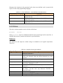
Table Of Contents
LIST OF ILLUSTRATIONS .................................................................................- 7 TABLES .............................................................................................................. - 7 EXAMPLE TABLES................................................................................................ - 8 FIGURES ............................................................................................................. - 9 EXAMPLE FIGURES ............................................................................................ - 10 -
PART I: A GENERAL INTRODUCTION
1. BASIC CONCEPTS.....................................................................................- 13 1.1 DEFINITION ................................................................................................. - 13 1.2 HISTORICAL BACKGROUND .......................................................................... - 13 1.3 FEASIBILITY OF AUTOMATING THE COMPILER CONSTRUCTION PROCESS......... - 14 -
2. THE COMPILER CONSTRUCTION LIFECYCLE................................................- 16 2.1 FRONT AND BACK ENDS .............................................................................. - 16 2.2 BREAKING DOWN THE WHOLE PROCESS INTO PHASES .................................. - 18 -
2.2.1 The Analysis Phases........................................................................... - 19 2.2.1.1 Linear (Lexical) Analysis ....................................................................- 19 2.2.1.2 Hierarchical (Syntactic) Analysis ........................................................- 20 2.2.1.3 Semantic Analysis................................................................................- 21 -
2.2.2 The Synthesis Phases ......................................................................... - 21 2.2.2.1 Intermediate Code Generation .............................................................- 21 2.2.2.2 Code Optimization...............................................................................- 21 2.2.2.3 Final Code Generation .........................................................................- 21 -
2.2.3 Meta-Phases....................................................................................... - 22 2.2.3.1 Symbol-Table Management.................................................................- 22 2.2.3.2 Error Handling .....................................................................................- 22 -
3. PROBLEM DEFINITION ...............................................................................- 23 3.1 HISTORICAL BACKGROUND .......................................................................... - 23 3.2 COMPILER CONSTRUCTION TOOLKITS: W HY?................................................ - 23 3.3 PRACTICAL AUTOMATION OF COMPILER W RITING PHASES ............................. - 24 3.4 MOTIVATION ................................................................................................ - 26 -
4. RELATED WORK .......................................................................................- 27 4.1 SCANNER GENERATORS – LEX.................................................................... - 27 4.2 PARSER GENERATORS – YACC .................................................................... - 28 4.3 FLEX AND BISON ......................................................................................... - 28 4.4 OTHER TOOLS............................................................................................. - 29 4.5 CONCLUSION .............................................................................................. - 31 -
5. OUR OBJECTIVE .......................................................................................- 32 6. DOCUMENT ORGANIZATION .......................................................................- 33 -
PART II: TECHNICAL DETAILS
1. ARCHITECTURE AND SUBSYSTEMS ............................................................- 35 2. THE LEXICAL ANALYSIS PHASE .................................................................- 38 -
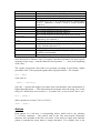
2.1 MORE ABOUT LEXICAL ANALYSIS .................................................................. - 38 -
2.1.1 Definition ........................................................................................... - 38 2.1.2 Lexical Tokens ................................................................................... - 38 2.1.3 Regular Expressions .......................................................................... - 40 2.1.4 Deterministic Finite Automata........................................................... - 42 2.1.5 Nondeterministic Finite Automata..................................................... - 43 2.2 LEXCELLENT: AN INTRODUCTION ................................................................. - 45 2.3 THE INPUT STREAM ..................................................................................... - 46 -
2.3.1 Unicode Problems.............................................................................. - 46 2.3.1.1 What is Unicode?.................................................................................- 46 2.3.1.2 The Problem.........................................................................................- 46 2.4 INPUT FILE FORMAT ..................................................................................... - 49 -
2.4.1 Top File Definition............................................................................. - 49 2.4.2 Class Definition ................................................................................. - 53 2.4.3 Rules................................................................................................... - 53 2.4.4 Extended Definitions (1) .................................................................... - 55 2.4.5 Extended Definitions (2) .................................................................... - 56 2.5 INPUT FILE ERROR HANDLING ...................................................................... - 56 2.6 THOMPSON CONSTRUCTION ALGORITHM ...................................................... - 63 2.7 SUBSET CONSTRUCTION ALGORITHM ........................................................... - 69 -
2.7.1 The Basic Idea.................................................................................... - 69 2.7.2 The Implementation ........................................................................... - 70 2.7.3 Contribution....................................................................................... - 72 2.8 DFA MINIMIZATION ...................................................................................... - 74 2.9 DFA COMPRESSION .................................................................................... - 77 -
2.9.1 Redundancy Removal Compression................................................... - 78 2.9.2 Pairs Compression............................................................................. - 78 2.10 THE GENERATED SCANNER ....................................................................... - 79 -
2.10.1 The Transition Table........................................................................ - 80 2.10.1.1 No Compression ................................................................................- 80 2.10.1.2 Redundancy Removal Compression ..................................................- 81 2.10.1.3 Pairs Compression .............................................................................- 81 -
2.10.2 The Input Mechanism....................................................................... - 82 2.10.2.1 Constructor.........................................................................................- 82 2.10.2.2 Data Members....................................................................................- 83 2.10.2.3 Methods .............................................................................................- 83 -
2.10.3 The Driver........................................................................................ - 84 2.10.4 The Lexical Analyzer Class.............................................................. - 86 2.10.4.1 Constructors .......................................................................................- 86 2.10.4.2 Constants............................................................................................- 86 2.10.4.3 Data Members....................................................................................- 87 2.10.4.4 Methods .............................................................................................- 87 2.11 HELPER TOOLS ......................................................................................... - 87 -
2.11.1 Graphical GTG Editor..................................................................... - 87 2.11.1.1 Definition ...........................................................................................- 88 2.11.1.2 Why GTGs? .......................................................................................- 89 2.11.1.3 GTG to Regular Expression: The Algorithm.....................................- 90 2.11.1.4 Implementation Details......................................................................- 92 2.11.1.5 Geometric Issues................................................................................- 93 -
3. THE PARSING PHASE ................................................................................- 98 3.1 MORE ABOUT PARSING ................................................................................ - 98 -
3.1.1 A General Introduction ...................................................................... - 98 -
3.1.2 Advantages of using Grammars......................................................... - 99 3.1.3 Syntax Trees vs. Parse Trees ........................................................... - 100 3.2 RECURSIVE DESCENT PARSERS ................................................................. - 101 3.3 LL(1) PARSERS ......................................................................................... - 107 -
3.3.1 Definition ......................................................................................... - 107 3.3.2 Architecture of an LL Parser ........................................................... - 107 3.3.3 Constructing an LL(1) Parsing Table.............................................. - 109 3.4 INPUT FILE FORMAT ................................................................................... - 110 -
3.4.1 Input File Syntax: The Overall Picture............................................ - 111 3.4.2 Input File Syntax: The Details ......................................................... - 111 3.4.3 Resolvers .......................................................................................... - 113 3.4.4 Comments......................................................................................... - 113 3.4.5 The LL(1) Input File Differences ..................................................... - 114 3.5 INPUT FILE ERROR HANDLING .................................................................... - 114 -
3.5.1 Semantic Errors and Warnings........................................................ - 114 3.5.1.1 Warnings............................................................................................- 114 3.5.1.2 Errors .................................................................................................- 115 -
3.5.2 Syntactic Errors ............................................................................... - 116 3.6 SYNTACTIC ANALYZER GENERATOR FRONT-END (SAG-FE) ........................ - 117 -
3.6.1 Scanning the Input File.................................................................... - 117 3.6.1.1 Reserved Keywords ...........................................................................- 117 3.6.1.2 Macro Representation of Other Tokens .............................................- 118 3.6.1.3 Data Structure for Scanning...............................................................- 118 -
3.6.2 Parsing the Input File ...................................................................... - 119 3.6.2.1 Recursive Descent Parser Generator CFG .........................................- 119 3.6.2.2 LL(1) Parser Generator CFG .............................................................- 120 3.6.2.3 The Tree Data Structure.....................................................................- 121 3.6.2.4 Building an Optimized Syntax-Tree ..................................................- 124 3.6.2.5 Syntax Error Detection ......................................................................- 130 3.7 SYNTACTIC ANALYZER GENERATOR BACK-END (SAG-BE) .......................... - 131 -
3.7.1 Code Generation Internals - RD Parser Generator ........................ - 131 3.7.2 Code Generation Internals – LL(1) Parser Generator.................... - 133 3.8 HELPER TOOLS ......................................................................................... - 136 -
3.8.1 Left Recursion Removal ................................................................... - 136 3.8.1.1 The Input............................................................................................- 136 3.8.1.2 The Output .........................................................................................- 136 3.8.1.3 The Process ........................................................................................- 137 3.8.1.4 Generating the Output File.................................................................- 140 -
3.8.2 Left Factoring Tool .......................................................................... - 142 3.8.2.1 The Input............................................................................................- 142 3.8.2.2 The Output .........................................................................................- 142 3.8.2.3 The Process ........................................................................................- 143 -
PART III: CONCLUSION AND FUTURE WORK
1. LEXCELLENT .........................................................................................- 146 1.1 SUMMARY ................................................................................................. - 146 1.2 FUTURE W ORK .......................................................................................... - 147 -
2. PARSPRING ...........................................................................................- 148 2.1 SUMMARY ................................................................................................. - 148 2.2 FUTURE W ORK .......................................................................................... - 148 -
3. THE GENERAL CONCLUSION ...................................................................- 149 REFERENCES .............................................................................................- 150 BOOKS ........................................................................................................... - 150 URLS ............................................................................................................. - 150 -
APPENDICES
A. USER'S MANUAL....................................................................................- 153 B. TOOLS AND TECHNOLOGIES ...................................................................- 166 C. GLOSSARY ............................................................................................- 167 -
List Of Illustrations
Tables
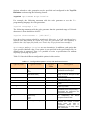
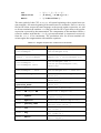
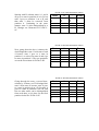
TABLE II-1: CONFIGURABLE OPTIONS IN TOP FILE DEFINITION SECTION............- 50 TABLE II-2: TOP FILE DEFINITION – USER-DEFINED-CODE PLACEMENT ............- 53 TABLE II-3: CLASS DEFINITION – USER-DEFINED-CODE PLACEMENT ................- 53 TABLE II-4: REGULAR EXPRESSION PATTERNS ...............................................- 54 TABLE II-5: EXTENDED DEFINITIONS (1) – USER-DEFINED-CODE PLACEMENT ...- 56 TABLE II-6: EXTENDED DEFINITIONS (2) – USER-DEFINED-CODE PLACEMENT ...- 56 TABLE II-7: REGULAR EXPRESSION CONTEXT-FREE GRAMMAR........................- 65 TABLE II-8: CODESTREAM CLASS DATA MEMBERS .........................................- 83 TABLE II-9: CODESTREAM CLASS METHODS ..................................................- 83 TABLE II-10: LEXICAL ANALYZER CLASS CONSTANTS ......................................- 86 TABLE II-11: LEXICAL ANALYZER CLASS DATA MEMBERS ................................- 87 TABLE II-12: LEXICAL ANALYZER CLASS METHODS .........................................- 87 TABLE III-1: MACRO REPRESENTATION OF TOKENS ......................................- 118 TABLE A-1: MAIN TOOLBAR DETAILS ...........................................................- 167 -
Example Tables
EXTAB 2-1: RESERVED WORDS AND SYMBOLS ...............................................- 38 EXTAB 2-2: EXAMPLES OF NONTOKENS .........................................................- 39 EXTAB 2-3: EXAMPLE REGULAR EXPRESSIONS ..............................................- 41 EXTAB 2-4: OPERATORS OF REGULAR EXPRESSIONS .....................................- 41 EXTAB 2-5: MORE EXAMPLES ON REGULAR EXPRESSIONS..............................- 42 EXTAB 2-6A: DFA STATE TABLE ...................................................................- 71 EXTAB 2-6B: DFA STATE TABLE ...................................................................- 72 EXTAB 2-6C: DFA STATE TABLE ...................................................................- 72 EXTAB 2-7A: DFA NEXT-STATE TABLE ..........................................................- 71 EXTAB 2-7B: DFA NEXT-STATE TABLE ..........................................................- 71 EXTAB 2-8A: DFA TRANSITION MATRIX .........................................................- 75 EXTAB 2-8B: DFA TRANSITION MATRIX .........................................................- 75 EXTAB 2-8C: DFA TRANSITION MATRIX .........................................................- 76 EXTAB 2-8D: DFA TRANSITION MATRIX .........................................................- 76 EXTAB 2-8E: DFA TRANSITION MATRIX .........................................................- 76 EXTAB 2-8F: DFA TRANSITION MATRIX .........................................................- 77 -
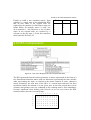
Figures
FIGURE I-1: THE COMPILER, ABSTRACTLY ......................................................- 13 FIGURE I-2: THE COMPILER CONSTRUCTION PROCESS ...................................- 16 FIGURE I-3: INTERMEDIATE REPRESENTION ....................................................- 17 FIGURE I-4: THE W HOLE PICTURE .................................................................- 18 FIGURE II-1: THE GENERAL ARCHITECTURE ....................................................- 35 FIGURE II-2: LEXCELLENT AND PARSPRING – THE MAIN COMPONENTS ............- 37 FIGURE II-3: LEXCELLENT – THE PROCESS....................................................- 45 FIGURE II-4: LEXCELLENT – THE FORMAT OF THE INPUT FILE ..........................- 49 FIGURE II-5: NFA FOR A ONE-SYMBOL REGEX ...............................................- 66 FIGURE II-6: NFA FOR TWO ORED REGEX'S ..................................................- 66 FIGURE II-7A: NFA FOR TWO CONCATENATED REGEX'S .................................- 66 FIGURE II-7B: NFA FOR TWO CONCATENATED REGEX'S .................................- 66 FIGURE II-8: NFA FOR A REGEX CLOSURE .....................................................- 67 FIGURE II-9: NFA FOR THE EMPTY W ORD ......................................................- 67 FIGURE II-10: NFA FOR A REGEX POSITIVE CLOSURE ....................................- 67 FIGURE II-11: NFA FOR AN OPTIONAL REGEX ................................................- 68 FIGURE II-12A: CLASS DIAGRAM FOR THE COMPRESSED DFA .........................- 77 FIGURE II-12B: CLASS DIAGRAM FOR THE COMPRESSED DFA .........................- 80 FIGURE II-13: THE DRIVER FLOWCHART.........................................................- 85 FIGURE II-14: REGEX AS A GTG ...................................................................- 88 FIGURE II-15: THE "C-COMMENT" REGULAR LANGUAGE ..................................- 89 FIGURE II-16: THE "EVEN-EVEN" REGULAR LANGUAGE ...................................- 90 FIGURE III-1: PARSER-LEXER INTERACTION ....................................................- 99 FIGURE III-2: ARCHITECTURE OF A TABLE-BASED TOP-DOWN PARSER ...........- 107 FIGURE III-3: PARSPRING – THE SYNTAX OF THE INPUT FILE .........................- 111 FIGURE III-4: THE PARSER GENERATOR FRONT-END ....................................- 117 FIGURE III-5: RD PARSER GENERATOR CODE GENERATION CLASS DIAGRAM .- 136 FIGURE III-6: LL1 PARSER GENERATOR CODE GENERATION CLASS DIAGRAM - 138 FIGURE III-7: SYNTAX ANALYZER HELPER TOOLS .........................................- 139 FIGURE III-8: LEFT-RECURSION-REMOVAL TOOL ..........................................- 140 FIGURE III-9: LEFT-FACTORING TOOL ..........................................................- 145 -
Example Figures
EXFIG 2-1: AN EXAMPLE DFA ......................................................................- 43 EXFIG 2-2: AN EXAMPLE NFA ......................................................................- 44 EXFIG 2-3: AN EXAMPLE NFA WITH Ε-TRANSITIONS .......................................- 44 EXFIG 2-4: NFA OF THE REGEX (A B C) .........................................................- 68 EXFIG 2-5: REDUNDANT OR AVOIDANCE ........................................................- 68 EXFIG 2-6: NFA FOR ( A * | B ) ......................................................................- 70 EXFIG 2-7: THE FINAL DFA .........................................................................- 72 E XFIG 2-8: IDENTIFIER NFA .........................................................................- 73 EXFIG 2-9: IDENTIFIER DFA – THE TRADITIONAL ALGORITHM ..........................- 73 EXFIG 2-10: IDENTIFIER DFA – THE ENHANCED ALGORITHM ...........................- 74 EXFIG 2-11: A TRANSITION MATRIX SUITABLE FOR COMPRESSION...................- 77 EXFIG 2-12: REDUNDANCY REMOVAL COMPRESSION .....................................- 78 EXFIG 2-13: PAIRS COMPRESSION ................................................................- 79 EXFIG 2-14: EXAMPLE GTG .........................................................................- 88 EXFIG 2-15A: CONVERTING THE "C-COMMENT" REGEX TO THE CORRESPONDING
GTG....................................................................................................- 91 EXFIG 2-15B: CONVERTING THE "C-COMMENT" REGEX TO THE CORRESPONDING
GTG....................................................................................................- 92 EXFIG 2-15C: CONVERTING THE "C-COMMENT" REGEX TO THE CORRESPONDING
GTG....................................................................................................- 92 EXFIG 2-15D: CONVERTING THE "C-COMMENT" REGEX TO THE CORRESPONDING
GTG....................................................................................................- 92 EXFIG 2-15E: CONVERTING THE "C-COMMENT" REGEX TO THE CORRESPONDING
GTG....................................................................................................- 92 EXFIG 2-16: THE GUI OF THE GTG EDITOR – STATES ....................................- 93 EXFIG 2-17: THE GUI OF THE GTG EDITOR – EDGES .....................................- 94 EXFIG 2-18: FINDING THE ENDPOINTS OF AN EDGE.........................................- 94 EXFIG 2-19A: THE EDGE-CLICKING PROBLEM ................................................- 96 EXFIG 2-19B: THE EDGE-CLICKING PROBLEM ................................................- 96 EXFIG 2-19C: THE EDGE-CLICKING PROBLEM ................................................- 97 EXFIG 3-1: SYNTAX TREE ...........................................................................- 101 -
Part II
Part
A General Introduction
1. Basic Concepts
1.1 Definition
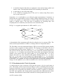
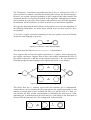
A compiler is a program that reads a program written in one language – the source
language – and translates it into an equivalent program in another language – the
target language. It can be simply stated alternatively, that a compiler is a program that
produces itself as an output if it were fed itself as an input!
Source Language
Target Language
Error Messages
Figure I-1: The Compiler, Abstractly
1.2 Historical Background
Compilers have been used since the very beginning of inventing the computers, and
have taken several shapes with varying ranges of complexity. Primarily, they were
invented to facilitate writing programs, because the only language that a computer
comprehends – the binary language (mere zeroes and ones) – are extremely
unreadable by humans, and early programmers exerted tremendous efforts just writing
the simplest of programs we run today.
Early computers did not use compilers; because they had just a few opcodes and a
confined amount of memory. Users had to enter binary machine code directly by
toggling switches on the computer console/front panel.
During the 1940s, programmers found that the tedious machine code could be denoted
using some mnemonics (assembly language) and computers could translate those
mnemonics into machine code. The primitive compiler, assembler, emerged.
During the 1950s, machine-dependent assembly languages were still found not to be
that ideal for programmers; and high level, machine-independent programming
languages evolved. Subsequently, several experimental compilers were developed (for
example, the seminal work by Grace Hopper [49] on the A-0 language), but the
FORTRAN team led by John Backus at IBM is generally credited as having
introduced the first complete compiler in 1957. Three years later, COBOL – an early
language to be compiled on multiple architectures – emerged [39].
The idea of compilation quickly caught on, and most of the principles of compiler
design were developed during the 1960s.
Programming languages emerged as a compromise between the needs of humans and
the needs of machines. With the evolution of programming languages and the
increasing power of computers, compilers are becoming more and more complex to
bridge the gap between problem-solving modern programming languages and the
various computer systems, aiming at getting the highest performance out of the target
machines.
Early compilers were written in assembly language. The first self-hosting compiler (a
compiler capable of compiling its own source code in a high-level language) was
created for Lisp by Hart and Levin at MIT in 1962. The use of high-level languages
for writing compilers gained added impetus in the early 1970s when Pascal and C
compilers were written in their own languages. Building a self-hosting compiler is a
bootstrapping problem [1] – the first such compiler for a language must be compiled
either by a compiler written in a different language, or (as in Hart and Levin's Lisp
compiler) compiled by running the compiler on an interpreter.
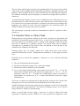
1.3 Feasibility of Automating the Compiler Construction Process
Compiler writing is a very complex process that spans programming languages,
machine architectures, language theory, algorithms and software engineering.
Although a few people are likely to build or even maintain a compiler for a major
programming language, the ideas and techniques used throughout the compiler
writing process (or the compiler construction process – I'll use the two terms
interchangeably) are widely applicable to general software design.
May be the first question that may come into the reader's mind is: Do we have a new
programming language every day? Programming languages – though numerous – are
limited to a few hundreds, most of which are already running and whose compilers
have been well-tested and optimized… so why do we need to automate the compiler
construction process? And is it worth the effort and time exerted doing that?
The following address these – and other questions – regarding the feasibility of
automating the compiler construction process, or at least, some of its phases [2]:
(1) The systematic nature of some of its phases.
The variety of compilers may appear overwhelming. There are hundreds of source
languages, ranging from traditional programming languages to specialized languages
(that have arisen in virtually every area of computer application). Target languages
are equally as varied; a target language may be another programming language or the
machine language of any computer between a microprocessor and a supercomputer.
Despite this apparent complexity, the basic tasks that any compiler must perform are
essentially the same. By understanding these tasks, we can construct compilers for a
wide variety of source languages and target machines using the same basic
techniques, and thus many phases of the compiler construction process are
automatable.
(2) The extreme difficulty encountered in implementing a full-fledged
compiler.
The first FORTRAN compiler – for example – took 18 staff-years to implement.
(3) The need for compilers in various applications, not only compilerrelated issues.
The string matching techniques for building lexical analyzers have also been used in
text editors, information retrieval systems, and pattern recognition programs. Contextfree grammars and syntax-directed definitions have been used to build many little
languages; such as the typesetting and figure drawing systems used in editing books.
In more general terms, the analysis portion (described shortly) in each of the
following examples is similar to that of a conventional compiler [2]:
I.
Text Formatters: A text formatter takes its input as a stream of characters,
most of which is text to be typeset, but some of which include commands
to indicate paragraphs, figures or mathematical structures like subscripts
and superscripts.
II.
Silicon Compilers: A silicon compiler has a source language that is similar
or identical to a conventional programming language. However, the
variables of the language represent not locations in memory, but logical
signals (0 or 1) or groups of signals in a switching circuit. The output is a
circuit design in an appropriate language.
III.
Query Interpreters: A query interpreter translates a predicate containing
relational and Boolean operators into commands to search a database for
records satisfying that predicate.
IV.
XML Parsers: The role of XML in modern database applications can't be
overestimated.
V.
Converting Legacy Data into XML: For updating legacy systems. This is an
extremely important application for large, old corporations with much data
that can't be lost when switching to newer systems.
VI.
Internet Browsers: This is one of the interesting applications that assures the
fact that the output of the process is not necessarily "unseen". In internet
browsers; the output is drawn to the screen.
VII. Parsing structured files: This is the most practical and widely used
application of parsers. Virtually any application needs to take its input
from a file. Once the structure of such a file is specified, a tool like ours
can be used to construct a parser easily (along with any parallel activity,
such as loading the contents of the file into memory) in a suitable data
structure.
VIII. Circuit burning applications using HDL specifications: This is another
example from the world of hardware.
IX. Checking spelling and grammar mistakes in word processing applications:
This is very common in commercial packages, like Microsoft Word®. The
importance of such an application stems from saving the great efforts
exerted when revising large, formal documents.
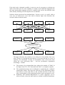
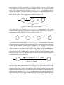
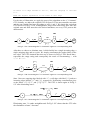
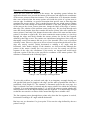
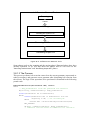
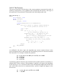
2. The Compiler Construction Lifecycle
Source Program
Analysis
Lexical Analysis
Front End
Error Handling
Symbol Table Management
Syntactic Analysis
Semantic Analysis
Intermediate Code Generation
Code Optimization
Back End
Code Generation
Synthesis
Target Program
Figure I-2: The Compiler Construction Process
2.1 Front and Back Ends
Often, the phases (described shortly) are collected into a front end and a back end.
The front end consists of those phases, or parts of phases, which depend primarily on
the source language and are largely independent of the target machine. These
normally include lexical and syntactic analysis, the creation of the symbol table,
semantic analysis, and the generation of intermediate code. A certain amount of code
optimization can be done by the front end as well. The front end also includes the
error handling that goes along with each of these phases.
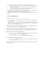
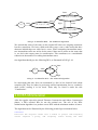
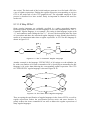
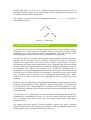
Intermediate Representation: A More-Than-Justified Overhead
It has become fairly routine to take the front end of a compiler and redo its associated
back end to produce a compiler for the same source language on a different machine.
If the back end is designed carefully, it may not even be necessary to redesign too
much of the back end. It is also tempting to compile several different languages into
the same intermediate language and use a common back end for the different front
ends, thereby obtaining several compilers for one machine.
Software design experience has mandated that; "whenever you're in trouble, add an
extra layer of abstraction". Let's start with an abstract figure that illustrates this
concept with no technical details:
Source 1
Source 2
Source 3
Source 4
Target 1
Target 2
Target 3
Target 4
Source 1
Source 2
Source 3
Source 4
Intermediate Form
Target 1
Target 2
Target 3
Target 4
Figure I-3: Intermediate Representation
The figure illustrates the problem we are facing if no intermediate form were
used. We have to redesign the back-ends for every front-end and vice versa. In
summary, the advantages of using an intermediate form; which more than
offsets the extra processing layer – and the performance degradation
accordingly – include:
(1)
The presence of an intermediate layer reduces the number of "links" in
the figure from N2 to 2*N. Note that each "link" is a complete compiler.
(2)
The optimization phase can be dedicated to optimizing the "standard"
intermediate format. This raises the efficiency of the optimization phase
and reduces its time and effort as the research increases in this area,
where certain phases of the optimization phase can be automated as well.
(3)
Portability and machine-independence in source languages can be
achieved easily, where the back-ends are realized on different platforms.
This approach is widely adopted nowadays; common examples include
Java TM and .NET-Compliant languages.
Now it's time to view the situation realistically:
Figure I-4: The Whole Picture
2.2 Breaking down the Whole Process into Phases
Conceptually, a compiler operates in phases, each of which transforms the source
program from one representation to another. There are two main categories of phases:
analysis and synthesis. Another category, which we prefer to name "meta-phases",
will be described shortly. The analysis part breaks up the source program into
constituent parts and creates an intermediate representation of it. The synthesis part
constructs the desired target program from the intermediate representation.
2.2.1 The Analysis Phases
2.2.1.1 Linear (Lexical) Analysis
The stream of characters making up the source program is read in a linear fashion (in
one direction, according to the language) and grouped into tokens – sequences of
characters having a collective meaning [3].
In addition to its role as an "input reader", a lexical analyzer usually handles some
"housekeeping chores" that simplify the remaining phases – especially the subsequent
phase; parsing [2]:
White space elimination:
Many languages allow "whitespace" (blanks, tabs, and newlines) to appear between
tokens. Comments can likewise be ignored by the parser as well as the translator, so
they may also be treated as white space.
Matching tokens with more than a single character:
The character sequence forming a token is called the lexeme for the token. Normally,
the lexemes of most tokens will consist of more than a character. For example,
anytime a single digit appears in an expression, it seems reasonable to allow an
arbitrary integer constant in its place. So the lexical analysis phase can't be simply
reading the input character by character (except in very special cases). In other words,
the character stream is usually different than the token stream.
Correlating error handling information with the tokens:
The lexical analyzer may keep track of the number of newline characters seen, so that
a line number can be associated with an error message.
Efficiency issues:
Since the lexical analyzer is the only phase of the compiler that reads the source
program character-by-character, it is possible to spend a considerable amount of time
in the lexical analysis phase, even though the later phases are conceptually more
complex. Thus, the speed of lexical analysis is a concern in compiler design [2].
Isolating anomalies associated with different encoding formats:
Input alphabet peculiarities and other device-specific anomalies can be restricted to
the lexical analyzer. The representation of special or non-standard symbols, such as ↑
in Pascal, can be isolated in the lexical analyzer.
There is much more stuff the lexical analyzer can handle, according to the specific
implementation at hand. The lexical analysis phase, together with the parsing phase, is
actually our concern. For that we defer a detailed description of both to two dedicated
chapters, in part II of this document. Consult section 6 in this part for more
information about the document organization.
2.2.1.2 Hierarchical (Syntactic) Analysis
It involves grouping the tokens of the source program into grammatical phrases that
are used by the compiler to synthesize output. Characters or tokens are grouped
hierarchically into nested collections with collective meaning; these nested collections
are what we call statements.
For any context-free grammar there is a parser that takes at most O(n3) time to parse a
string of n tokens [2]. However, this is very expensive when we engage into practical
applications. So, researchers have exerted intensive efforts to find "smarter"
techniques for parsing.
Most practical parsing methods fall into one of two classes, called the top-down and
bottom-up methods. These terms refer to the order in which nodes in the parse tree are
constructed. In the former, construction starts at the root and proceeds towards the
leaves, while in the latter, construction starts at the leaves and proceeds towards the
root. (A parse tree is a visual representation of the hierarchical structure of a
language statement, in which the levels in the tree depict the depth and breadth of the
hierarchy. We will have more to say about different types of trees later).
The popularity of top-down parsers is due to the fact that efficient parsers can be
constructed more easily by hand using top-down methods. Bottom-up parsing,
however, can handle a larger class of grammars and translation schemes.
Lexical Analysis vs. Parsing
I. The Rationale behind Separation
There are several reasons for separating the analysis phase of compiling into lexical
analysis and parsing, the most important of which are [2]:
1. Simpler design is perhaps the most important consideration. The separation of
lexical analysis from syntactic analysis often allows us to simplify one or the other of
these phases. For example, a parser embodying the conventions for comments and
whitespace is significantly more complex than one that can assume comments and
whitespace have already been removed by a lexical analyzer. If we are designing a
new language, separating the lexical and syntactic conventions can lead to a cleaner
overall language design.
2. Compiler efficiency is improved. A separate lexical analyzer allows us to
construct a specialized and potentially a more efficient processor for the task. A huge
amount of time is spent reading the source program and partitioning it into tokens.
Specialized buffering techniques for reading input characters and processing tokens
can significantly speed up the performance of a compiler.
3. Compiler portability is enhanced. Input alphabet peculiarities and other devicespecific anomalies can be restricted to the lexical analyzer. The representation of
special or non-standard symbols, such as ↑ in Pascal, can be isolated in the lexical
analyzer.
4. Specialized tools have been designed to help automate the construction of
lexical analyzers and parsers when they are separated. These tools are actually the
core of CCW, more about their importance, details and input specifications are
presented in the relevant chapters later in the document.
II. A Special Relation?
The division between lexical and syntactic analysis is somewhat arbitrary. One factor
in determining the division is whether a source language construct is inherently
recursive or not. Lexical constructs do not require recursion, while syntactic
constructs often do. The lexical analyzer and the parser form a producer-consumer
pair. The lexical analyzer produces tokens and the parser consumes them. Produced
tokens can be held in a token buffer until they are consumed. The interaction between
the two is constrained only by the size of the buffer, because the lexical analyzer
cannot proceed when the buffer is full and the parser cannot proceed when the buffer
is empty. Commonly, the buffer holds just one token. In this case, the interaction can
be implemented simply by making the lexical analyzer be a procedure called by the
parser, returning tokens on demand.
2.2.1.3 Semantic Analysis
Certain checks are performed to ensure that the components of a program fit together
meaningfully. The semantic analysis phase checks the source program for semantic
errors and gathers type information for the subsequent code-generation phase. It uses
the hierarchical structure determined by the syntax-analysis phase to identify the
operators and operands of expressions and statements.
2.2.2 The Synthesis Phases
2.2.2.1 Intermediate Code Generation
After syntax and semantic analysis, some compilers generate an explicit intermediate
representation of the source program. We can think of this intermediate representation
as an assembly program for an abstract machine.
2.2.2.2 Code Optimization
The code optimization phase attempts to improve the intermediate code, so that fasterrunning machine code will result. There is a great variation in the amount of code
optimization different compilers perform. In those that do the most – called
"optimizing compilers" – a significant fraction of the compilation time is spent on this
phase. However, there are simple optimizations that significantly improve the running
time of the target program without slowing down the compilation performance
noticeably.
2.2.2.3 Final Code Generation
Memory locations are selected for each of the variables used by the program. Then,
intermediate instructions are each translated into a sequence of machine instructions
that perform the same task. A crucial aspect is the assignment of variables to registers,
since the intermediate code is the same for all platforms and machines and should not
be dedicated to a specific one.
2.2.3 Meta-Phases
2.2.3.1 Symbol-Table Management
An essential function of a compiler is to record the identifiers used in the source
program and collect information about various attributes of each identifier. These
attributes may provide information about the storage allocated for an identifier, its
type, its scope (where in the program it is valid), and – in the case of procedure names
– such things as the number and types of its arguments, the method of passing each
argument (e.g. by reference), and the type returned, if any.
A symbol table is a data structure containing a record for each identifier, with fields
for the attributes of the identifier. The data structure allows us to find the record for
each identifier and to store or retrieve data from its record quickly.
2.2.3.2 Error Handling
Each phase can encounter errors. However, after detecting an error, a phase must
somehow deal with that error, so that the compilation can proceed, allowing further
errors in the source program to be detected. A compiler that stops when it finds the
first error is not as helpful as it could be.
The syntax and semantic analysis phases usually handle a large fraction of the errors
detectable by the compiler. The lexical phase can detect errors where the characters
remaining in the input do not form any token of the language. Errors where the token
stream violates the structure rules (syntax) of the language are determined by the
syntax analysis phase. During semantic analysis the compiler tries to detect constructs
that have the right syntactic structure but no meaning to the operation involved, e.g., if
we try to add two identifiers, one of which is the name of an array, and the other the
name of a procedure.
3. Problem Definition
3.1 Historical Background
At about the same time that the first compiler was under development, Noam
Chomsky [50] began his study of the structure of natural languages. His findings
eventually made the construction of the compilers considerably easier and even
capable of partial automation. Chomsky's studies lead to the classification of
languages according to the complexity of their grammars and the power of the
algorithms to recognize them. The Chomsky Hierarchy (as it's now called) [51]
consists of four levels of grammars, called the type 0, type 1, type 2 and type 3
grammars; each of which is a specialization of its predecessor. The type 2, or contextfree grammars, proved to be the most useful for programming languages – and today
they are the standard way to represent the structure of programming languages. The
study of the parsing problem (the determination of efficient algorithms for the
recognition of context-free languages) was pursued in the 1960s and 70s, and lead to a
fairly complete solution of this problem, which today has become a standard part of
compiler theory. Context-free languages and parsing algorithms are discussed in the
relevant chapters later in this document.
Closely related to context-free grammars are finite automata and regular expressions,
which correspond to Chomsky's type 3 grammars. Their study led to symbolic
methods for expressing the structure of words (or tokens). Finite automata and regular
expressions are discussed in detail in the chapter on lexical analysis.
As the parsing problem became well understood, a great deal of work was devoted to
developing programs that will automate this part of compiler development. These
programs were originally called compiler-compilers, but are more aptly referred to as
parser generators, since they automate only one part of the compilation process. The
best-known of these programs, Yacc (Yet Another Compiler-Compiler), was written
by Steve Johnson in 1975 for the UNIX system. Similarly, the study of finite
automata led to the development of another tool called a scanner generator, of which
LEX (developed for the UNIX system by Mike Lesk about the same time as Yacc) is
the best known.
During the late 1970s and early 1980s a number of projects focused on automating the
generation of other parts of compilers, including code generation. These attempts
have been less successful, possibly because of the complex nature of the operations
and our less-than-perfect understanding of them. For example, the automaticallygenerated semantic analyzers have a general performance degradation of 1000%!!
(This means that they run ten times slower than manually-written semantic analyzers).
3.2 Compiler Construction Toolkits: Why?
Is it worth automating the compiler writing process? The following – very briefly –
discusses the main difficulties a compiler writer encounters when writing a compiler
code manually:
• Compiler writing is a complex, error-prone task that needs much time and effort.
•
The resulting (manual) code is usually hard to debug and maintain.
•
The code walkthrough is hard due to the amount of the written code and the
diversity of the available implementations.
•
Any small modification in the specification of the compiler results in big changes
to the code, and subsequently to severe performance deterioration on the long run
as the structure of the code is continuously modified.
•
The class of algorithms that suits manual implementation of compilers is generally
inefficient.
For these and other problems, tremendous research efforts were exerted in the 1970s
and 80s to automate some phases of the compiler writing process. Following the
"bulletin board" convention used above; the following are some of the advantages that
a compiler writer gains when using compiler construction tools:
•
The developer is responsible only for providing the specifications. No tedious,
repeated work is required; thus avoiding the aforementioned difficulties.
•
Adopting the most efficient algorithms in its construction; thus providing the
developer with an easy means to generating efficient programs that would
otherwise have been too difficult to implement. Manually-written compilers have
proven to lack the required efficiency and maintainability.
•
Ease of maintenance. Only the specifications are to be modified if a desired
amendment is to be introduced.
•
Providing developers unfamiliar with the compiler theory with an access to the
uncountable benefits of using compiler writing techniques in compiler-unrelated
applications.
3.3 Practical Automation of Compiler Writing Phases
The compiler writer, like any programmer, can profitably use software tools such as
debuggers, version managers, and profilers … to implement a compiler. These may
include:
•
Structure Editors: A structure editor takes as an input a sequence of commands
to build a source program. The structure editor not only performs the text-creation
and modification functions of an ordinary text editor, but it also analyzes the
program text, putting an appropriate hierarchical structure on the source program.
Thus, the structure editor can perform additional tasks such as checking that the
input is correctly formed, supplying keywords automatically (such as supplying a
closing parenthesis for an opened one, or auto-completing reserved keywords),
and highlighting certain keywords. Furthermore, the output of such an editor is
often similar to the output of the analysis phase of a compiler; that is – imposing a
certain hierarchical structure on the input program.
•
Pretty Printers: A pretty printer analyzes a program and prints it in such a way
that the structure of the program becomes clearly visible. For example, comments
may appear in a special font, and statements may appear with an amount of
indentation proportional to the depth of their nesting in the hierarchical
organization of the statements.
Both of these tools are implemented in CCW 1.0.
In addition to these software-development tools, other more specialized tools have
been developed for helping implement various phases of a compiler. I mention them
briefly in this section; the tools implemented in CCW are covered in detail in the
appropriate chapters.
Shortly after the first compilers were written, systems to help with the compilerwriting process appeared. These systems have often been referred to as compilercompilers, compiler-generators, or translation-writing systems; as was discussed in
the historical background above. Largely, they are oriented around a particular model
of languages, and they are most suitable for generating compilers of languages similar
to the model.
For example, it is tempting to assume that lexical analyzers for all languages are
essentially the same, except for the particular keywords and signs recognized. Many
compiler-compilers do in fact produce fixed lexical analysis routines for use in the
generated compiler. These routines differ only in the list of keywords recognized, and
this list is all that's needed to be supplied by the user.
Some general tools have been created for the automatic design of specific compiler
components, these tools use specialized languages for specifying and implementing
the component, and many use algorithms that are quite sophisticated. The most
successful tools are those that hide the details of the generation algorithm and produce
components that can be easily integrated into the remainder of a compiler. The
following is a list of some useful compiler-construction tools:
I. Parser Generators. These produce syntax analyzers, normally from input that is
based on a context-free grammar. In early compilers, syntax analysis consumed not
only a large fraction of the running time of a compiler, but also a large fraction of the
intellectual effort of writing it. This phase is now considered one of the easiest to
implement. Many "little languages", such as PIC and EQN (used in typesetting
books), and any file with a definitive structure; were implemented in a few days using
parser generators. Many parser generators utilize powerful parsing algorithms that are
too complex to be carried out by hand.
II. Scanner Generators. These automatically generate lexical analyzers, normally
from a specification based on regular expressions. The basic organization of the
resulting lexical analyzer is in effect a finite automaton – both to be detailed soon.
III. Syntax-Directed Translation Engines. These produce collections of routines
that walk the parse tree, generating intermediate code. The basic idea is that one or
more "translations" are associated with each node of the parse tree, and each
translation is defined in terms of translations at its neighbor nodes in the tree.
IV. Automatic Code Generators. Such a tool takes a collection of rules that define
the translation of each operation of the intermediate language into the machine
language for the target machine.
3.4 Motivation
Among the aforementioned tools, the first two are the core of our project. There are a
number of reasons that restricted us to implementing these two, the most important of
which are:
•
Not all of these tools have gained wide acceptance due to the lack of efficiency,
standardization and practicality. As mentioned before, the semantic analyzers –
for example – generated automatically are about ten times slower than their adhoc counterparts.
•
Practical lexical analyzers and parsers are widely applicable to other fields of
application, unrelated to the compiler construction process. Page 8 contains some
of the applications a parser (together with its lexical analyzer) can be useful in.
•
The available lexical analyzers and parsers – though numerous – share some
drawbacks discussed in details in the next chapter on the market survey. We
decided to implement a tool that – as much as the time limit permits – avoid these
drawbacks.
4. Related Work
We have performed a survey on the currently available compiler construction toolkits.
It was found that the most significant tools available are LEX and Yacc. However,
numerous tools exist. Many of the disadvantages of LEX and Yacc were solved by
other tools. However, so far no single tool has solved all of the problems normally
encountered in such products. We are going to investigate some of them here:
4.1 Scanner Generators – LEX
As previously stated, lexical analyzer generators take as input the lexical
specifications of the source language and generate the corresponding lexical
analyzers. Different generator programs have different input formats and vary in
power and use. We shall describe here LEX, which is one of the most powerful and
widely used lexical analyzer generators. LEX was the first lexical analyzer generator
based on regular expressions. It is still widely used. It is the standard lexical analyzer
(scanner) generator on UNIX systems, and is included in the POSIX standard.
LEX reads the given input files, or its standard input if no file names are given, for a
description of a scanner to be generated. The description is in the form of pairs of
regular expressions and C code, called rules. After that, LEX generates as output a C
source file that implements the lexical analyzer. This file is compiled and linked to
produce an executable. When the executable is run, it analyzes its input for
occurrences of the regular expressions. Whenever it finds one, it executes the
corresponding C code.
Some Disadvantages of LEX
We have examined LEX from several perspectives and finally we were able to decide
the following drawbacks in it:
o The generated code is very complex and completely unreadable. Consequently, its
maintainability is low.
o The generated lexical analyzer can be generated only in the C language (Another
version of LEX has been developed to support object oriented code in C++, but it
is still under testing).
o There is only one DFA compression technique utilized.
o There is no clear interface between the scanner module and the application that is
going to use the module.
o It doesn't support Unicode, so the only supported language is English.
o Some of the header files used by the generated scanner are restricted to the UNIX
OS. Thus, its portability is low.
o It lacks a graphical user interface.
4.2 Parser Generators – Yacc
Syntactic analyzer generators take as an input the syntactic specifications of the target
language – in the form of grammar rules – and generate the corresponding parsers. It
holds for automated parser generation as well that different generator programs have
different input formats and vary in power and use. However, the variation here is
more acute due to the different types of parsers that might be generated (top-down
parsers vs. bottom-up parsers). We shall describe here Yacc, which is one of the most
powerful and widely used parser generators. Indeed, LEX and Yacc were designed so
that seamless effort is exerted in order to integrate the generated lexical analyzer and
the generated parser.
Yacc (Yet Another Compiler Compiler) is a general-purpose parser generator that
converts a grammar description for an LALR(1) context-free grammar into a C
program to parse that grammar. Yacc is considered to be the standard parser generator
on UNIX systems. It generates a parser based on a grammar written in the BNF
notation. Yacc generates the code for the parser in the C programming language.
Some Disadvantages of Yacc
The disadvantages of Yacc are almost the same as the disadvantages of LEX. They are
repeated here for convenience:
o The generated code is very complex and completely unreadable. Consequently, its
maintainability is low.
o The generated parser can be generated only in the C programming language
(Another version of Yacc has been developed to support object oriented code in
C++, but it is still under testing).
o There is only one type of parsers that may be generated which is the LALR(1)
bottom-up parser.
o There is no clear interface between the parser module and the application that is
going to use the module.
o Some of the header files used by the generated parser are restricted to the UNIX
OS. Thus, its portability is low.
o It lacks a graphical user interface.
4.3 Flex and Bison
LEX and Yacc have been replaced by Flex and Bison and, more recently, Flex++ and
Bison++. Such enhancements have solved the problems of portability and provided
the user with a means to generate object oriented compilers in C++ but still the rest of
the drawbacks remain.
4.4 Other Tools
Other than LEX and Yacc, we will make a brief survey on the available tools and
packages related to our product together with their drawbacks. The references [8] –
[30] are used in this section. We preferred not to attach every reference to its program
to avoid cluttering this page.
ANTLR
o Only the recursive descent parsing technique is supported.
o It has no graphical user interface.
o It has some problems with Unicode.
Coco/R
o The only parsing technique available is the LL table-based parsing technique.
o It doesn’t support Unicode.
o There is no graphical user interface.
Spirit
o
o
o
o
o
The only output language supported is C++.
Only the recursive descent parsing technique is supported.
There is no graphical user interface.
It doesn't support Unicode.
It doesn't provide a scanner generation capability.
Elkhound
o
o
o
o
o
The only output languages supported are C++ and Ocaml.
Only the bottom-up table based parsing technique is supported.
There is no graphical user interface.
It doesn't support Unicode.
It doesn't provide a scanner generation capability.
Grammatica
o The only parsing technique used is the recursive descent parsing technique.
o There is no graphical user interface.
o The scanner produced by its scanner generator is inefficient.
LEMON
o
o
o
o
o
The only output languages available are C and C++.
The only parsing technique is the LALR(1) table-based parsing technique.
There is no graphical user interface.
It doesn't provide a scanner generation capability.
It doesn't support Unicode.
SYNTAX
o It works only on the UNIX OS.
o There is no graphical user interface.
o The only output language available is C.
o Only the LALR(1) table-based parsing technique is supported.
o It doesn't support Unicode.
GOLD
o Only the LALR(1) table-based parsing technique is supported.
o Doesn't generate the driver programs (only the tables).
o There is no graphical user interface.
AnaGram
o The only output languages allowed are C and C++.
o Only the LALR(1) table-based parsing technique is supported.
o It doesn't support Unicode.
SLK
o Only the LL(k) table-based parsing technique is supported.
o There is no graphical user interface.
Rie
o
o
o
o
The only output language available is C.
Only the LR table-based parsing technique is supported.
There is graphical user interface.
It doesn't support Unicode.
Yacc++
o
o
o
o
The only output language available is C++.
Only the ELR(1) table-based parsing technique is supported.
There is no graphical user interface.
It doesn’t support Unicode.
ProGrammar
o It uses a separate ActiveX layer which degrades performance.
o It is not clear what type of parsing technique it uses.
YaYacc
o
o
o
o
o
o
The only output language available is C++.
The only parsing technique available is LALR(1) table based parsing.
It works only on FreeBSD.
It doesn't have a graphical user interface.
It doesn't support Unicode.
It doesn’t provide a scanner generation capability.
Styx
o The only output language available is C.
o Only the LALR(1) table-based parsing technique is supported.
o It doesn't have a graphical user interface.
PRECC
o
o
o
o
The only output language available is C.
Only the LL table-based parsing technique is supported.
There is no graphical user interface.
It doesn't support Unicode.
YAY
o
o
o
o
o
The only output language available is C.
Only the LALR(2) table-based parsing technique is supported.
There is no graphical user interface.
It doesn't support Unicode.
There is scanner generation capability.
Depot4
o
o
o
o
The only output languages available are Java and Oberon.
The only parsing technique available is recursive descent parsing.
There is no graphical user interface.
There is no scanner generation capability.
LLGen
o
o
o
o
o
The only output language available is C.
Only the ELL(1) table-based parsing technique is supported.
There is no scanner generation capability.
It doesn't support Unicode.
There is no graphical user interface.
LRgen
o
o
o
o
o
It is designed so that the output is mainly written in C++.
The only parsing technique is LALR(1) table based parsing.
It is a commercial application.
There is no Unicode support.
There is no graphical user interface.
4.5 Conclusion
Most of the available tools don’t provide the choice among table-based and recursive
descent parsing. And it is rare to find a tool with a graphical user interface. Such a
tool is usually a commercial one (i.e., it costs a lot of money).
Unicode support is also missing in most of the tools surveyed. Also we can notice that
only a few tools support multilingual code generation. That is, other than C and C++,
it is not common to find a non-commercial tool that fulfills your needs.
Some tools do provide a scanner generator besides the parser generator, but as we've
just seen; this is not always the case.
5. Our Objective
As it's now obvious from the previous section, there are a number of common
drawbacks shared by most of the available products. Most of the parser generators
implement a single parsing technique, or at most two. Most of them are mere console
applications, without a user interface. Unicode is supported in a few of them; even
those tools that support Unicode suffer from some shortcomings that make them
generally unpractical. Code generation is usually in one or two languages. Scanner
generators are sometimes existent, but most often you have to implement them
yourself.
So we've decided to develop a tool that overcomes most of these drawbacks. Because
of the time limit, we adopted extensibility as a principal paradigm, so that – for
example – the LR parsing technique can be introduced in version 2.0 easily, even
though version 1.0 currently supports recursive descent and LL(1) parsing techniques
only. Unicode is supported in version 1.0, and some demos are available on the
companion CD illustrating Arabic applications. Code generation is currently
supported in three languages; namely ANSI C++, C# and Java. It's a trivial matter to
add a new language, as will be illustrated in details in the chapter on parsing later in
the document. LEXcellent, our lexical analyzer generator, is available to support its
companion, ParSpring, the parser generator.
Our interface for integrating the process is CCW (Compiler Construction
Workbench), a user friendly interface that supports most of the nice features
introduced in IDEs, such as syntax highlighting, line numbers, breakpoints and
matching brackets. More advanced features such as auto-completion are included in
the future work plan. It's expected that version 2.0 is to eliminate all the drawbacks
evident in most commercial applications. Currently, version 1.0 eliminates about 80%
of them, given the extensible framework it's based upon.
6. Document Organization
After the field and the problem have been introduced, we turn now to briefly
discussing the organization of this document.
Part I – which the reader has probably surveyed before reaching this section – mainly
introduces the topic and clarifies the overall picture. Chapters 1 and 2 discuss the
basic concepts. The problem is defined precisely in chapter 3. A market survey is
carried out in chapter 4, and chapter 5 discusses our objective from implementing our
tool.
Part II, which is the bulk of this document, is dedicated essentially to those developers
who will use our tool, together with those interested in any implementation details.
Chapter 1 contains mainly a block diagram depicting the overall system architecture,
together with a brief discussion of each component.
Chapter 2 is dedicated to the lexical analysis phase. Section 1 is an introduction;
augmenting what was presented in the 'Basic Concepts' chapter in Part I. Section 2
introduces LEXcellent; our lexical analyzer generator. Section 3 discusses its input
stream, and sections 4 and 5 are dedicated to its input file format. Sections 6, 7, 8 and
9 illustrate in full details the algorithms used in our implementation for LEXcellent.
Section 10 is dedicated to describing the generated lexical analyzer. Section 11
describes the graphical GTG editor; which is a helper tool used to create regular
expressions easily via a sophisticated graphical user interface.
Chapter 3 is dedicated to the parsing phase. Sections 1, 2 and 3 are introductory; again
augmenting the material presented in Part I. Sections 4 and 5 are dedicated to the
input file format of ParSpring, the parser generator. Sections 6 and 7 are pure
implementation details. Finally, two helper tools are discussed in section 8.
Part III finalizes the document by providing the general conclusion; together with a
summary for each tool and its future work plan. Then the tools, technologies and
references used in this project are listed. The appendices are attached to the end of the
document.
This document may be used by more than one reader. If you are new to the whole
issue, the following sections in Part I are recommended for first reading: 1.1, 1.3, 2.1,
2.2, 3.1, 3.2, 3.3, 5, and sections 2.1, 3.1, 3.2 and 3.3 in Part II.
If you know what you want to do, and you prefer to start using the tool directly; read
the following in Part II: 2.4, 2.5, 3.4 and 3.5. Section 2.10 will be useful also; though
not necessary to get started. Don't forget the user manual in the appendices.
For using the helper tools, consult sections 2.11 and 3.8 in Part II.
Finally, when you're done using the tool; you may want to take a look at the
implementation details – and you're welcome to augment our work. The source code
is provided on the companion CD. Sections 2.3, 2.6, 2.7, 2.8 and 2.9 discuss in full
details the implementation details for LEXcellent. Its companion's details are outlined
in sections 3.6 and 3.7.
Part II
Part
II
Technical Details
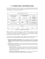
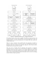
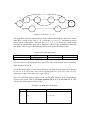
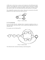
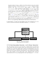
1. Architecture and Subsystems
Our Compiler Construction Toolkit consists of several components that interact with
each other to facilitate the process of compiler development. The general architecture
of the package can be represented in figure II-1:
Figure II-1: The General Architecture
While the IDE was developed using the .NET platform, almost all the other
components of the system were developed in native C++. Such combination allowed
us to gain the powerful GUI capabilities of the .NET framework without sacrificing
the efficiency and portability of the C++ unmanaged code.
The following is a brief investigation of each component in the system. Each of these
components is to be fully detailed in a dedicated chapter later in the document.
•
Integrated Development Environment: It the environment in which the compiler
developer creates and maintains projects, edits specification files, uses the utilities
and helper tools and invoke the scanner and parser generator tools to generate his
compiler.
•
Lexical Analyzer Generator: It is the software component that is responsible for
generating the lexical analyzer (scanner), given the user specifications. It consists
of the following general modules:
o Input File Parser: This module is responsible for parsing the specifications
file that contains the regular definitions of the tokens to be returned by the
generated scanner. The regular definitions are converted into an NFA then into
a DFA. More on both later.
o Optimization (Minimization/Compression): This module is responsible for
optimizing the produced DFA obtained from the previous phase.
o Scanner Code Generator: This module is responsible for generating the
source code of the required scanner.
•
Syntactic Analyzer Generator: It is the software component that is responsible for
generating the syntactic analyzer (parser), given the user specifications. It consists
of the following general modules:
o Input File Parser: This module is responsible for parsing the specifications
file that contains the grammar specifications of the language to be recognized
by the generated parser. The grammar rules are converted into a tree inside the
program memory.
o LL(1) Parser Code Generator: If the user specifies that the generated parser
should be an LL(1) parser, then this module should assume responsibility for
generating the parser.
o Recursive-Descent Parser Code Generator: If the user specifies that the
generated parser should be a recursive-descent parser, then this module should
assume responsibility for generating the parser.
•
Helper Tools: A set of tools that facilitates the process of writing the
specifications of the desired scanner and parser. They are mainly invoked from the
IDE.
o GTG to Regular Expression Converter: A tool that gives the developer the
capability to specify his regular definition in terms of a Generalized Transition
Graph instead of a regular expression. This may be easier in some cases.
o Regular Expression Manipulator: A tool that allows the developer to
generate new regular expressions from the union, intersection or negation of
input regular expressions.
o Left Factoring/Left Recursion Removal: A tool that performs left factoring
and left recursion removal on a given CFG, which are two essential operations
that must be performed if a recursive-descent parser is to be generated. Such
facility frees the developer from doing all that effort manually.
•
Back End: It is the set of classes that generate the required scanners and parsers in
any of the supported languages. Currently, only C++, C# and Java are available,
but more languages may be supported easily.
Figure II-2 gives a brief illustration of the two main components of the system, the
scanner generator LEXcellent and the parser generator ParSpring. This block diagram
is just for reference, more details about both tools are presented in the appropriate
chapters later in this part.
Figure II-2: LEXcellent and ParSpring – The Main Components
The package consists of three main executables: The IDE, the scanner generator and
the parser generator. The user runs the IDE to start his development, to create and
maintain projects, to edit the specification files in a tailored editor and to utilize the
available helper tools.
When it is time to generate code, the IDE invokes the appropriate executable to
generate a scanner or a parser, as required by the user. If the operations succeed, the
generated code will be released in a code file, otherwise a list of errors will be
returned from the code generator to the IDE.
Thus, the process of dealing with the underlying code generators is completely
transparent to the user. However, the user has the choice whether to use our IDE to
invoke the scanner and parser generators, to use another IDE (such as the Visual
Studio IDE) or to invoke the generators directly without an IDE. Our IDE, however,
offers a group of functionalities and utilities that makes it the best choice for dealing
with the scanner and parser generators.
2. The Lexical Analysis Phase
2.1 More about Lexical Analysis
2.1.1 Definition
Lexical analysis is usually the first phase of the compilation process in which the
lexical analyzer takes a stream of characters and produces a stream of names,
keywords, and punctuation marks that the parser uses for syntax analysis. In addition,
it may discard whitespace and comments between the tokens to simplify the operation
of later phases. It would unduly complicate the parser to have to account for possible
whitespace and comments at every possible point; this is one of the main reasons for
separating lexical analysis from parsing. For example [2], in lexical analysis the
characters in the assignment statement
position := initial + rate * 60
would be grouped into the following tokens:
1. The identifier position.
2. The assignment symbol :=.
3. The identifier initial.
4. The plus sign +.
5. The identifier rate.
6. The multiplication sign *.
7. The number 60.
The blanks separating the characters of these tokens would normally be eliminated
during lexical analysis.
2.1.2 Lexical Tokens
A lexical token is a sequence of characters that can be treated as a unit in the grammar
of the source language [3]. Lexical tokens are usually classified into a finite set of
token types. For example, some of the token types of a typical programming language
are listed in the table below.
Some tokens have special meaning in programming languages such as IF, VOID and
RETURN. These are called reserved words and, in most languages, cannot be used as
identifiers. Some of these are illustrated in ExTab 2-1 on the next page.
ExTab 2-1: Reserved words and symbols
Type
ID
IF
COMMA
NOTEQ
LPAREN
RPAREN
NUM
REAL
Examples
foo n14 last
if
,
!=
(
)
73 0 00 515 082
66.1 .5 10. 1e67 5.5e-10
The input file might contain sequences of characters that are either ignored by the
lexical analyzer or not tackled by the language grammar. These are called nontokens.
Examples of nontokens are illustrated in ExTab 2-2.
ExTab 2-2: Examples of nontokens
comment
preprocessor directive
preprocessor directive
macro
blanks, tabs, and newlines
/* try again */
#include<stdio.h>
#define NUMS 5, 6
NUMS
In languages weak enough to require a macro preprocessor, the preprocessor operates
on the source character stream, producing another character stream that is then fed to
the lexical analyzer. It is also possible to integrate macro processing with lexical
analysis.
Given a program such as
float match0(char *s) /* find a zero */
{
if (!strncmp(s, "0.0", 3))
return 0.;
}
the lexical analyzer will return the stream
FLOAT
LBRACE
COMMA
RETURN
ID(match0)
LPAREN
CHAR
STAR
ID(s)
RPAREN
IF
LPAREN
BANG
ID(strncmp)
LPAREN
ID(s)
STRING(0.0)
COMMA
NUM(3)
RPAREN
RPAREN
REAL(0.0)
SEMI
RBRACE
EOF
where the token-type of each token is reported; some of the tokens, such as identifiers
and literals, have semantic values attached to them, giving auxiliary information in
addition to the token-type. For example, the second identifier is attached the string
“match0”.
There many ways to describe the lexical rules of a programming language. For
example, we can use English to describe the lexical tokens of a language. A
description of identifiers in C or Java is provided on the following paragraph [1]:
An identifier is a sequence of letters and digits; the first character must be a letter. The
underscore (_) counts as a letter. Uppercase and lowercase letters are different. If the
input stream has been parsed into tokens up to a given character, the next token is
taken to include the longest string of characters that could possibly constitute a token.
Blanks, tabs, newlines and comments are ignored except as they serve to separate
tokens. Some whitespace is required to separate otherwise adjacent identifiers,
keywords, and constants.
A more compact, precise, and formal way to specify the lexical tokens of a source
language makes use of the formal language of regular expressions. Not only can
automated checks be performed on this form of specification, but it can be used to
generate efficient lexical analyzers as well.
2.1.3 Regular Expressions
Regular expressions provide a mathematical way to specify patterns. Each pattern
matches a set of strings. So, a regular expression will stand for a set of strings. Before
providing a definition for regular expressions, we define some of the technical terms
that will be used again and again during the discussion of lexical analysis and regular
expressions.
The term alphabet or character class denotes any finite set of symbols. Typical
examples of symbols are letters and characters. The set {0, 1} is the binary alphabet.
ASCII and EBCDIC are two examples of computer alphabets.
A string over some alphabet is a finite sequence of symbols drawn from that alphabet.
In language theory, the terms sentence and word are often used as synonyms for the
term "string" [2]. The length of a string s, usually written as |s|, is the number of
occurrences of symbols in s. For example, banana is a string of length six. The empty
string, denoted by ε, is a special string of length zero.
The term language denotes any set of strings over some fixed alphabet. This
definition is very broad. Abstract languages like •, the empty set, or {ε}, the set
containing only the empty string, are languages under this definition. If A and B are
two languages over some fixed alphabet, then we define the concatenation of the two
languages A.B is a language defined by:
A.B = {xy: x ∈ A and y ∈ B}
k
0
L refers to k concatenations of the language L. If k = 0, then L contains only the
empty word ε. The Kleene Closure of a language L denoted by L* is the language
containing all strings that can obtained by forming zero or more concatenations of
words from L, or mathematically:
∞
L* =
U
Li.
i=0
A regular expression describing a given language L over some alphabet Σ can be any
of the following [1]:
•
•
•
•
•
•
If a is a symbol in Σ (a ∈ Σ), then a is a regular expression with L(a) = { a }.
ε, where L(ε) = { ε } (The empty string).
If r is a regular expression over Σ, then (r) is a regular expression over Σ, with
L( (r) ) = L(r).
If r is a regular expression over Σ, then r* is a regular expression over Σ, with
L(r*) = L*(r).
If r and s are regular expressions over Σ, then their concatenation, r.s or
simply r s, is a regular expression over Σ, with L(r s) = L(r).L(s).
If r and s are regular expressions over Σ, then their union, r | s is a regular
expression over Σ, with L(r | s) = L(r) U L(s).
A language is regular if and only if it can be specified by a regular expression. Some
regular expressions and descriptions of the languages they define are listed as
examples in ExTab 2-3:
ExTab 2-3: Example regular expressions
(0 | 1)* 0
Binary numbers that are multiples of two.
b* ( a b b* )* ( a | ∊ ) Strings of a's and b's with no consecutive a's.
( a | b )* a a ( a | b )* Strings of a's and b's containing consecutive a's.
In writing regular expressions, we will sometimes omit the concatenation symbol, and
we will assume that Kleene closure "binds tighter" than concatenation, and
concatenation binds tighter than alternation; thus the regular expression a b | c means
(a . b) | c, and the regular expression ( a | b c * ) means a | ( b . (c)* ).
ExTab 2-4: Operators of regular expressions
a
∊
M|N
M.N
MN
"a.+*"
M*
M?
+
M
[a − zA − Z]
.
An ordinary character stands for itself.
The empty string. Another way to write it.
Alternation, choosing from M or N.
Concatenation, an M followed by an N.
Another way to write concatenation.
Quotation, a string in quotes stands for itself
literally.
Repetition (zero or more times).
Optional, zero or one occurrence of M.
Repetition, one or more times.
Character set alternation.
A period stands for any single character
except newline.
Next, we present some of the useful abbreviations that are commonly used to write
regular expressions. [abcd] means (a | b | c | d), [b-g] means [bcdefg], [b-gM-Qkr]
+
means [bcdefgMNOPQkr], M? means (M | ∊), and M means (M · M*). These
extensions are convenient, but none of them extend the descriptive power of regular
expressions: Any set of strings that can be described using these abbreviations could
also be described using the basic set of operators. All the operators are summarized in
ExTab 2-4 on the previous page.
Using this language, we can specify the lexical tokens of a programming language as
follows:
ExTab 2-5: More examples on regular expressions
if
[a-zA-Z_][a-zA-Z_0-9]*
[0-9]+
([0-9]+"."[0-9]*)|([0-9]*"."[0-9]+)
("\\"[a-z]*"\n")|(" "|"\n"|"\t")+
.
IF
ID
NUM
REAL
no token, just white space
error
The fifth entry of ExTab 2-5 recognizes comments or whitespace but does not report
back to the parser. Instead, the white space is discarded and the lexical analysis
process is resumed. The comments for this lexical analyzer begin with two slashes,
contain only alphabetic characters, and end with a newline.
Finally, a lexical specification should be complete, always matching some initial
substring of the input; we can always achieve this by having a rule that matches any
single character (and in this case, prints an illegal character error message and
continues).
These rules are a bit ambiguous. For example, if8 can be matched as a single
identifier or as the two tokens if and 8. Moreover, the string if can be considered an
identifier or a reserved word. There are two important disambiguation rules to resolve
such ambiguities that are used by LEXcellent:
•
Longest match: The longest initial substring of the input that can match any
regular expression is taken as the next token.
•
Rule priority: For a particular longest initial substring, the first regular
expression that can match determines its token-type. This means that the order of
writing down the regular-expression rules has significance.
Thus, if8 matches as an identifier by the longest-match rule, and if matches as a
reserved word by rule-priority.
2.1.4 Deterministic Finite Automata
A deterministic finite automaton consists of [2]:
1. A finite set of states, often denoted by Q.
2. A finite set of input symbols, often denoted by Σ.
3. A transition function that takes as arguments a state and an input symbol and
returns a state. The transition function will commonly be denoted δ.
4. A start state q0, one of the states in Q.
5. A set, of final or accepting states F. The set F is a subset of Q. There can be
zero or more states in F.
Sometimes, it is comfortable to use informal graph representation of automata, in
which states are represented by circles or nodes, and the transition from a give state qi
to state qj on symbol a is represented by a directed edge from state (node) qi to state
(node) qj, labeled with a. The start state is marked by an incoming edge, and
accepting states are marked by an extra inner circle inside the node.
ExFig 2-1 is a graph representation of a DFA with Σ = {a, b}:
ExFig 2-1: An example DFA
A deterministic finite automaton will often be referred to by its acronym: DFA. The
most succinct representation of a DFA is a listing of the five components above.
The first thing we need to understand about a DFA is how the DFA decides whether
or not to accept a sequence of input symbols. The language of the DFA is the set of
all strings that the DFA accepts. Suppose al a2 ... an is a sequence of input symbols.
We start out with the DFA in its start state, q0. We consult the transition function δ,
say δ(q0, a1) = q1 to find the state that the DFA enters after processing the first input
symbol a1.We process the next input symbol, a2, by evaluating δ(q1, a2); let us
suppose this state is q2. We continue in this manner finding states q3, q4 ... qn where
δ(qi-1, ai) = qi, for each i. If qn is a member of F, then the input a1, a2 … an is accepted,
and if not then it is rejected. The set of all strings that the DFA accepts is the language
of that DFA. For example, the DFA in the figure above accepts the language of all
strings over the alphabet {a, b} with even number of a’s and even number of b’s.
2.1.5 Nondeterministic Finite Automata
A nondeterministic finite automaton (NFA) has the power to be in several states at
once. This ability is often expressed as an ability to "guess" something about its input.
It guesses which state to go next such that if there is a sequence of guesses that leads
the string to be accepted by the machine, then this sequence of guesses is chosen by
the NFA. We introduce the formal notions associated with nondeterministic finite
automata. The differences between DFAs and NFAs will be pointed out as we do.
An NFA consists of [2]:
1. A finite set of states, often denoted Q.
2. A finite set of input symbols, often denoted Σ.
3. A start state q0, one of the states in Q.
4. F, a subset of Q, is the set of final (or accepting) states.
5. The transition function δ is a function that takes a state in Q and an input
symbol in Σ or the empty word ε as arguments and returns a subset of Q.
Notice that the only difference between an NFA and a DFA is in the type of
value that δ returns: a set of states in the case of an NFA and a single state in
the case of a DFA.
Here is an example of an NFA:
ExFig 2-2: An example NFA
In the start state, on input character a, the automaton can move either right or left. If
left is chosen, then strings of a's whose length is a multiple of three will be accepted.
If right is chosen, then even-length strings will be accepted. Thus, the language
recognized by this NFA is the set of all strings of a's whose length is a multiple of two
or three.
On the first transition, the machine in ExFig 2-2 must choose which way to go. It is
required to accept the string if there is any choice of paths that will lead to acceptance.
Thus, it must "guess", and must always guess correctly.
Edges labeled with ∊ may be taken without using up an input symbol. ExFig 2-3 is
another NFA that accepts the same language:
ExFig 2-3: An example NFA with ∊-transitions
Again, the machine must choose which ∊-edge to take. If there is a state with some ∊edges and some edges labeled by symbols, the machine can choose to eat an input
symbol (and follow the corresponding symbol-labeled edge), or to follow an ∊-edge
instead.
2.2 LEXcellent: An Introduction
LEXcellent is the component responsible for generating the lexical analyzer based on
the specifications given in an input file. Since lexical analysis is the only phase in a
compiler that deals with input files, special care should be given to dealing with
Unicode streams.
The main components of LEXcellent are illustrated here. This is just a general
overview and a thorough description of each phase of the generation process is
provided in the appropriate sections of this chapter.
Figure II-3: LEXcellent – The Process
2.3 The Input Stream
The input stream is represented by the class LexerInputReader. This class
encapsulates all the fields and methods necessary for reading and parsing the input
file. The class was designed principally to deal with Unicode files. Its functionalities
can be summarized in two main functions:
•
Read the user options (such as the output language and the compression
technique) and pass it to the following phases to control the scanner generation
process.
•
Parse the regular definitions and produce the corresponding NFAs. Constructing
an NFA from a regular definition should be a straight forward task. The NFAs are
then grouped into a single NFA to be passed to the next stage.
2.3.1 Unicode Problems
One of the main features of LEXcellent is its ability to deal with the Unicode character
set, and to generate lexical analyzers capable of dealing with Unicode. This
guarantees that LEXcellent will have a widespread use because most systems are now
Unicode-enabled and commercial lexical analyzer generators generally lack this
feature.
2.3.1.1 What is Unicode?
Unicode [34] is an industry standard designed to allow text and symbols from all of
the writing systems in the world to be consistently represented and manipulated by
computers. Unicode characters can be encoded using any of several schemes termed
Unicode Transformation Formats (UTF).
The Unicode Consortium has as its ambitious goal the eventual replacement of
existing character encoding schemes with Unicode, as many of the existing schemes
are limited in size and scope, and are incompatible with multilingual environments. Its
success in unifying character sets has led to its widespread and predominant usage in
the internationalization and localization of computer software. The standard has been
implemented in many recent technologies, including XML, the Java programming
language, and modern operating systems.
2.3.1.2 The Problem
Since we have chosen to use the C++ programming language in the implementation of
LEXcellent, and to restrict ourselves to the ANSI standards; we have used the
IOStream library to implement the input and the output. The input to LEXcellent is
the text file containing the description of the lexical analyzer. The output is the
generated lexical analyzer, along with errors (if any) and the statistics of the
construction process.
Changing the definition of a certain macro converts the program from the ASCII build
mode to the Unicode build mode. This switches the program from using narrow
characters and their related character processing functions and IOStream classes to
using wide characters and their related character processing functions and IOStream
classes. Narrow-character programs tend to be faster and smaller. If the user needs are
limited to narrow characters, it would be an overhead to use a Unicode program. On
the other hand, the user might want to develop a set of programs for the Arabic
language or the Chinese language, for instance. So, a Unicode-enabled lexical
analyzer generator will be great. Consequently, two builds will be available: an ASCII
release and a Unicode release.
During the development process, the program was compiled and tested under the
ASCII build. When the application was complete, it was the time to try the Unicode
build. We thought defining the aforementioned macro would get things work as
expected. Unicode-encoded test files were prepared and all what remained was to
build the application under Unicode. It was true that the application compiled
successfully with no problems, but it failed to read the input files of all test cases. The
failures ranged from detecting invalid sequence of characters at the beginning of the
file to reading spurious null before or after each character. When the input included
Arabic letters, nothing related to Arabic was processed. We tried the same files with
simple programs developed with C# and faced no problem.
We started to write simple, “Hello World” text files under different Unicode
encodings and use binary editors to view the contents of these files. We found that all
Unicode files always begin with a fixed sequence of bytes that are independent of the
actual text stored in the file. The bytes in that sequence differ according to the
encoding under use. We correctly concluded that this was to help the application
determine the specific encoding under use in the file. But this was not enough to tell
how to solve the problem.
Indeed, this problem exhausted an excessive amount of time from us. Such a problem
was never expected. See references [40] – [48] for more about this problem. We made
a research plan for the whole matter. The plan was organized as a set of questions to
be answered as follows:
-
What are the different encodings used to represent Unicode?
How does IOStream internally work and how does it deal with wide
characters and different file encodings?
How did other tools deal with Unicode?
The answer to the first question is quite long and is beyond the scope of this
document. The answer of the second question is the topic of many books merely
dedicated to the IOStream library. For the third question, we were not surprised with
the number of forums and websites that tackled the topic. However, we shall briefly
and collectively illustrate the results of the three questions and the solution of the
problem in the following outline [35].
•
C++ IOStream classes use some type of encoder/decoder classes to convert
between the internal representation of characters and their external
representation. If the characters are externally encoded using some encoding
scheme, then an appropriate encoder/decoder object should be ‘imbued’ with
the stream object.
•
The most famous Unicode encodings are UTF-8, UTF-16 BE, and UTF-16
LE. UTF-32 BE and LE are not as famous. UTF-8 is an 8-bit, variable-width
encoding, compatible with ASCII that uses one to four bytes per character.
UTF-16 is a 16-bit, variable-width encoding that uses from two to four bytes
per character. UTF-16 is available in two flavors: Little-Indian and BigIndian; which differ in the ordering of bytes in each character. UTF-32 is 32bit fixed-width encoding that is available either as Little-Indian or Big-Indian.
UTF-32 encodings are less commonly used.
•
The C++ standard library has not implemented encoder/decoder classes for
Unicode encodings. It defines the template, but does not implement it. The
C++ standard library implements something like a fake encoder/decoder class
for dealing with wide characters. All it has to do is to convert a two-byte
character into a single byte when writing to a file (or the opposite if reading
from a file). If this is not bad enough, how this conversion is performed is
implementation-dependent.
•
The number of characters in the Unicode character set exceeds 65,536. Thus, a
Unicode character needs more than two bytes for storage. Despite this fact, a
wide character variable in Microsoft Visual C++.NET 2003™ takes only two
bytes. Thus, some characters took more than two bytes in memory. This
means that in-memory characters have variable lengths.
•
We were able to find implementations of the encoder/decoder classes for
UTF-8 and UTF-16 LE. When it was the time to retry the testing process, we
found that it is the responsibility of the developer to determine which encoding
scheme is used in the text file, and ‘imbue’ the appropriate encode/decoder
object to deal with before opening the file. This means that the file must be
opened twice, once to determine its encoding and another to read it.
•
Microsoft Visual C++.NET 2003™ implementation of IOStream library is not
that good. It works very well with IOStream classes based on narrow
characters, but it fails miserably to operate with wide characters and different
‘imbued’ encoder/decoder objects. The most predominant failure occurs when
trying to reposition the read pointer (seek) although the address sought is
given as an absolute address rather than a relative one. The latter feature is
crucial for any lexical analyzer to be able to deal with arbitrary lookaheads.
The last observation was extremely painful to us, since it meant that we had to either
stop trying to support the Unicode character set or to find an alternative method to
process the input. In addition, any alternative method for processing the input should
comply with the standards; otherwise our top goal (which is platform independence)
is to be sacrificed.
At last, we decided to make our own input classes that wrapped the C file I/O routines
included in the C++ standard library. The input classes we have developed support
UTF-8, UTF-16 BE and UTF-16 LE. The application was then tested under the
Unicode build over Unicode test files and it operated smoothly and without problems.
We implemented a successful sample application that deals with the Arabic language.
You can view it on the companion CD.
2.4 Input File Format
The input file format of LEXcellent is very similar to that of LEX. This is because
LEX is widely used and its input format explained in many compiler books. Thus,
anyone familiar with LEX should be able to use LEXcellent with little trouble.
The LEXcellent input file consists of five sections, a line beginning with %% separates
each two:
Top File Definition
%%
Class Definition – User Code
%%
Rules
%%
Extended Definitions (1) – User Code
%%
Extended Definitions (2) – User Code
Figure II-4: LEXcellent – The Format of the Input File
The specializations of these sections differ depending on the programming language
used for code generation. For example, the 'Extended Definitions (1)' section specifies
user code to be copied into the generated files. If the lexical analyzer is to be
generated in C++, this section will be copied onto the top of the C++ source code file
(.cpp file). If the lexical analyzer is to be generated in C#, this section will be copied
onto the C# source code file (.cs file) just after the lexical analyzer class definition but
inside the same namespace.
Each section is detailed below.
2.4.1 Top File Definition
This section can be used for the following purposes:
•
•
•
Specifying options related to code generation.
Declaring macros for latter use in the specification.
Writing some code that is placed, as-is, at the top of the generated file.
These can be specified in any order, and can be mixed together in the specification. In
addition, comments can be freely added anywhere in this section and are copied
without changes to the generated code. There are two types of comments:
i) Single-line comments. The line should begin with //
ii) Comments delimited by /* */. The delimiters should be placed at the
beginning of the line without any indentation. Otherwise, their effect is
ignored.
The format of each of the above purposes is detailed below:
Options
Options related to code generation can be specified and configured in the Top File
Definition section using the following format:
%option OptionName = OptionValue
For example, the following statement tells the code generator to use the C++
programming language for code generation:
%option Language = C++
The following statement tells the code generator that the permitted range of Unicode
characters is from 0x0000 to 0x007F:
%option CharacterSet = [\d0-\d127]
Lines describing options should be unindented. Otherwise, it will be considered userdefined code that should be copied as-is into the generated code. This anomaly is
found in the LEX input file format, too. That's why we preferred not to modify it.
OptionName and OptionValue are case insensitive. In addition, each option has
a pre-specified default value. If an option is not specified in the specification file, its
default value is assumed. Thus, it is possible to write a specification file without
explicitly specifying any option.
Table II-1 lists the different configurable options in this section:
Table II-1: Configurable Options in Top File Definition Section
Option Name
Language
Option Values
Default
Value
Description
C++
C#
Java
Character class
(described below)
C++
The programming language of the
generated lexical analyzer.
[d0-d127]
Namespace
Identifier
Compiler
ClassName
FunctionName
Identifier
Identifier
LexicalAnalyzer
ReturnType
Identifier
int
FileName
Name and path of the file
Lex
CompressionTechniqu
e
None
Redundancy
Pairs
Best
A nonnegative integer
Redundancy
The subset of Unicode character
range to use for the input of the
lexical analyzer.
The namespace of the generated
lexical analyzer class.
The lexical analyzer class name.
The pattern matching function
name.
The Return type of the pattern
matching function.
The path and name of the
generated lexical analyzer file(s) –
Appropriate file extensions are
appended automatically.
The compression technique to use
for compressing the lexical
analyzer transition table.
CharacterSet
PairsThreshold
GetNextToken
8
If pairs compression is used, this
specifies the number of items
above which, the state is
considered
dense
and
is
represented by an array rather
than a linked list.
InvalidTokenAction
Value to be returned by
the function.
-2
EOFAction
Value to be returned by
the function.
-1
If the lexical analyzer faced an
invalid token, then the pattern
matching function returns by
executing:
return InvalidTokenAction;
If the lexical analyzer reaches the
end of file, then the pattern
matching function returns by
executing:
return EOFAction;
Macros
Macros provide a way to give frequently used regular expressions more user-friendly
names for later use. They help improve readability as well as maintainability of the
specification. Indeed, macros provide a way for centralizing the changes; i.e. if we
have a macro used in more than one regular expression and it is required to change the
value of this macro, then the change is made only at the macro definition statement.
This section contains declarations of simple macro definitions to simplify the scanner
specification. Macro definitions have the form:
MacroName Definition
The MacroName is a word beginning with a letter or an underscore ('_') followed by
zero or more letters, digits, or '_'. The Definition is to begin at the first nonwhite-space character following the name and continuing to the end of the line. For
example,
DIGIT
[0-9]
The definition can subsequently be referred to using {MacroName}, which will
expand to (Definition). It is possible to invoke previously defined macros in the
definition of the current macro. For example,
DIGIT
LETTER
ID
[0-9]
[a-zA-Z]
{LETTER}({LETTER}|{DIGIT})*
defines DIGIT to be a regular expression which matches a single digit, LETTER to
be a regular expression which matches an English letter (either in upper-case or
lower-case), and ID to be a regular expression which matches a letter followed by
zero-or-more letters or digits. A subsequent reference to
{DIGIT}+"."{DIGIT}*
is identical to
([0-9])+"."([0-9])*
and matches one-or-more digits followed by a '.' followed by zero-or-more digits.
Lines describing macros should be unindented. Otherwise, it will be considered userdefined code that should be copied as-is into the generated code. This anomaly is
found in the LEX input file format, too. That's why we preferred not to modify it.
User-Defined Code
This is the code to be copied as-is into the generated file. Indented lines represent
user-defined code, which is copied in order into the generated code. An alternative is
to delimit a section of code by %{ %} (copied as-is into the generated code after
removing the delimiters). For example,
#include <iostream>
%{
#include <cmath>
using namespace std;
%}
These will be copied to the top of the generated header file as follows:
#include <iostream>
#include <cmath>
using namespace std;
The delimiters are to be placed at the beginning of the line. Otherwise, they will be
ignored. The exact location in the generated code where user-defined code is pasted
differs depending on which programming language the code uses. The following table
illustrates the location in the generated code where user-defined code is pasted with
respect to the used programming language.
Table II-2: Top of Definition – User Defined Code Placement
Programming Language
C++
Java
C#
Location
At the top of the header file (.h).
At the top of the source file (.java).
At the top of the source file (.cs).
2.4.2 Class Definition
In this section, the user writes code to be placed inside the lexical analyzer class
definition. For a C++ developer, this allows declaring member variables, member
functions, static variables and/or static functions. For a C#/Java developer, this allows
declaring member/static variables and defining member/static functions. The code is
copied as-is into the generated code.
The exact location in the generated code where user-defined code is pasted differs
depending on which programming language the code uses. The following table
illustrates the location in the generated code where user-defined code is pasted with
respect to the used programming language.
Table II-3: Class Definition – User Defined Code Placement
Programming Language
C++
Location
Inside the lexical analyzer class definition, in the
header file (.h).
Inside the lexical analyzer class definition, in the
source file (.java).
Inside the lexical analyzer class definition, in the
source file (.cs).
Java
C#
2.4.3 Rules
The rules section contains a series of rules of the form:
pattern
action
where pattern must be unindented and the action must begin on the same line. A
detailed discussion of patterns and actions is provided below.
Patterns
The patterns in the input are written using an extended set of regular expressions.
These are:
Table II-4: Regular Expression Patterns
Regular Expression
X
.
[xyz]
[abj-oZ]
[ab[-]
[^A-Z]
[^]
[^A-Z\n]
[]
Description
match the character x
any character except newline (Note that any character
means any character from the defined character set in the
options)
a "character class"; in this case, the pattern matches either
an x, a y, or a z
a "character class" with a range in it; matches an a, a b, any
letter from j through o, or a Z
a "character class"; in this case, the pattern matches either
a, b, [, or -.
a "negated character class", i.e., any character but those in
the class. In this case, any character EXCEPT an
uppercase letter.
match ^
any character EXCEPT an uppercase letter or a newline
an empty word; a[]b matches ab
r*
r+
r?
{Macro}
\x
"[xyz]\"foo"
\O12
\o12
\x43F
\X1212FF
\D48
\d434344
(r)
rs
R | s
zero or more r's, where r is any regular expression
one or more r's
zero or one r's (that is, "an optional r")
the expansion of the "Macro" definition
if x is an a, b, f, n, r, t, or v, then the ANSI-C interpretation
of L'\x'. Otherwise, a literal x (used to escape operators
such as *)
the literal string: [xyz]"foo
the Unicode character with octal value 12
the Unicode character with octal value 12
the Unicode character with hexadecimal value 0x043F
the Unicode character with hexadecimal value 0x1212
followed by two capital F's.
the Unicode character with decimal value 48
the Unicode character with decimal value 43434 followed
by the Unicode character L'4'
match an r; parentheses are used to override precedence
the regular expression r followed by the regular expression
s; called "concatenation"
either regular expression r or regular expression s
Note that inside a character class, all regular expression operators lose their special
meaning except escape \ and the character class operators, -, ], and, at the beginning
of the class, ^.
The regular expressions listed above are grouped according to precedence, higher
precedence first. Those grouped together have equal precedence. For example,
foo | bar*
is the same as
(foo) | (ba(r*))
since the * operator has higher precedence than concatenation, and concatenation is
higher than alternation |. This pattern therefore matches either the string "foo" or the
string "ba" followed by zero-or-more r's. To match "foo" or zero-or-more "bar"'s, use:
foo | (bar)*
and to match zero-or-more "foo"'s-or-"bar"'s:
(foo | bar)*
Actions
Each pattern in a rule has a corresponding action, which can be any arbitrary
C++/C#/Java statement. The pattern ends at the first non-escaped whitespace
character; the remainder of the line is its action. If the action is empty, then when the
pattern is matched the input token is simply discarded. For example, here is the
specification for a regular expression, which deletes all occurrences of the single-line
C++ comment from the input:
"//".*
If the action contains a {, then the action spans until the balancing } is found, and the
action may cross multiple lines. LEXcellent knows about strings and comments and
will not be fooled by braces found within them. Actions are allowed to begin with %{
and will consider the action to be all the text up to the next %} (regardless of ordinary
braces, comments, and strings inside the action).
2.4.4 Extended Definitions (1)
This section and the next are optional and the input file may be terminated without
specifying them. This section is used to write code that is placed as-is into the
generated files. Thus, no syntactic checks are performed on the contents of this
section.
For a C++ developer, the code in this section is placed at the top of the generated
source (.cpp) file. This can be used to include header files, declare/define external
and/or static variables and define macros. For Java and C# developers, the code in this
section is placed right after the end of the definition of the lexical analyzer class, but
inside the same namespace. This can be used to define other classes, structures, and
enumerations under the same namespace. The following table summarizes the
placement of the code in the generated files according to the programming language
under use.
Table II-5: Extended Definitions (1) – User Defined Code Placement
Programming
Language
Location
C++
Java
At the top of the generated source file (.cpp).
Right after the end of the lexical analyzer class, but inside the
same namespace in the generated source file (.java).
Right after the end of the lexical analyzer class, but inside the
same namespace in the generated source file (.cs).
C#
2.4.5 Extended Definitions (2)
This section is also used to write code that is placed without modifications into the
generated files. Hence, the tool does not perform syntactic checks on the contents of
this section.
For a C++ developer, the code in this section is placed at the end of the generated
source (.cpp) file. Thus, it can be used to implement any member functions declared
in the 'Class Definition' section or add any required code. For C# and Java developers,
the code is placed at the bottom of the generated source file, after the end of the
namespace. This can be used to define other namespaces along with their classes. The
following table summarizes the placement of the code in the generated files according
to the programming language used.
Table II-6: Extended Definitions (2) – User Defined Code Placement
Programming
Language
Location
C++
Java
At the bottom of the generated source file (.cpp).
At the bottom of the generated source file, right after the
namespace of the lexical analyzer class (.java).
At the bottom of the generated source file, right after the
namespace of the lexical analyzer class (.cs).
C#
2.5 Input File Error Handling
In this section, we describe the error messages that LEXcellent provides for various
types of errors encountered in input files, and indicate some of the situations that
cause such errors.
Unexpected End of File.
Causes
The input file terminates before defining the Rules section.
Example
The following sample generates the specified error.
%option CharacterSet = [\x00-\x7F]
%option Language = C++
sin (S|s)(I|i)(N|n)
%%
Bad Directive.
Causes
The Top File Definition section contains an invalid directive. The three valid
directives are
o
%option name = value.
This line specifies modifying the value of an option such as the language to be
used for code generation. Although the option name is not case-sensitive, the
keyword option is case-sensitive.
o
%{
This begins a block of code that will be placed as-is in the generated file. This
block is terminated by %}. For further information, see “LEXcellent Input File
Format”.
o
%%
This terminates the Top File Definition section.
Example
The following sample includes two lines that generate the specified error.
%option CharacterSet = [\x00-\x7F]
/* The following line is valid. */
%option LanGuage = C++
/* The following line is invalid. */
%OPTION ClassName = Lexer
/* The following line is invalid. */
%unknown_directive
Invalid Option Specification.
Proper option format:
%option some_thing = some_value.
Causes
The option format is invalid.
Example
The following sample includes three lines that generate the specified error.
%option CharacterSet = [\x00-\x7F]
/* The following line is invalid. */
%option
/* The following line is invalid. */
%optionLanguage = C++
/* The following line is invalid. Missing = */
%option ClassName Lexer
The Specified Option is not Supported.
Causes
Although the format of the option is valid, it specifies an unsupported option.
Example
The following sample includes three lines that generate the specified error.
%option CharacterSet = [\x00-\x7F]
/* The following line is invalid. */
%option Lang = C++
/* The following line is invalid. */
%OPTION aBrandNewOption = Lexer
/* The following line is invalid. */
%option Class Name = Lexer
Invalid Macro Definition. Eliminate the Trailing Characters.
Causes
The macro definition is followed by spurious characters.
Example
The following sample generates the specified error.
%option CharacterSet = [\x00-\x7F]
%option Language = C++
Macro1 [a-z]+
/* A valid line. */
/* The following line is invalid. */
InvMacro [0-9]+ spurious characters are the cause of the error
The Specified Macro Name is Already Defined.
Causes
The user is trying to redefine a macro.
Example
The following sample generates the specified error.
%option CharacterSet = [\x00-\x7F]
%option Language = C++
/* The following line is valid. */
Macro1 [a-z]+
/* The following line is invalid. */
Macro1 [0-9]+
The Invoked Macro is Undefined.
Causes
The user invokes a macro within a regular expression that has not been defined.
Example
The following sample includes three lines that generate the specified error.
%option CharacterSet = [\x00-\x7F]
%option Language = C++
/* The following two lines are valid. */
Macro1 [a-z]
Macro2 {Macro1}+
/*The following line is invalid*/
Macro3 {Macro4}+
Macro4 (a|b)*
/*The following line is invalid due to self-reference*/
Macro5 a|{Macro5}
%%
/*Top class definition*/
%%
/* The following definition is invalid */
[0-9]{UndefinedMacro}
{
cout<<”I
am
invoking
undefined macro.”<<endl; }
an
%%
Invalid Macro Invocation within the Regular Expression. The Macro
Name Contains Invalid Characters.
Causes
The name of the macro invoked by the user is not a valid identifier. The valid
format for a macro name is:
[a-zA-Z_][a-zA-Z_0-9]*
Example
The following sample includes two lines that generate the specified error.
%option CharacterSet = [\x00-\x7F]
%option Language = C++
/* The following two lines are valid. */
GoodMacro [a-z]
BadOrGoodMacro {Macro1}+
/*The following two lines are invalid*/
Macro3 {Good Macro}+
Macro4 {Bad|GoodMacro}+
Bad Character Set Definition. Check the Supplied %option
Character Set.
Causes
The user specifies an invalid character set. If the user does not specify a
character set to use in the input file, then the default character set (ASCII [\x00-
\x7F]) is assumed. Otherwise, the valid format for character sets is the same as
that for a valid character class.
Example
The following samples generate the specified error.
/* The following line is invalid */
%option CharacterSet = ][
/* The following line is invalid. Unexpected end of character
class*/
%option CharacterSet = [\x00-\x7F
Invalid Use of Parentheses within the Regular Expression. Check
Balancing.
Causes
The user has put a spurious closing parenthesis ")" inside the regular expression.
Example
The following sample generates the specified error.
%option CharacterSet = [\x00-\x7F]
%option Language = C++
%%
%%
/* The following regular definition is invalid. */
(a|b)*)abcd
{ cout<<”I am closing something that I did not
open.”<<endl; }
Unexpected End of the Regular Expression. Check Balance of
Parentheses.
Causes
The user has opened one or more parentheses and the regular expression has
terminated before balancing them.
Example
The following sample includes two lines that generate the specified error.
%option CharacterSet = [\x00-\x7F]
%option Language = C++
%%
%%
/* The following regular definition is invalid. */
((a|b)*
{ cout<<”The regex should have terminated with
)”<<endl; }
/* The following regular definition is valid. */
\((a|b)*
{ cout<<”The first ( is escaped is by
the
backslash.”<<endl; }
Unexpected End of Regular Expression.
Causes
The user has opened double quotes “ but has forgotten to close them. It may be
the case also that the user has opened a character class [ but has forgotten to
close it. Finally, the user might have tried to invoke a macro but have forgot the
closing brace }.
Example
The following sample includes three lines that generate the specified error.
%option CharacterSet = [\x00-\x7F]
%option Language = C++
%%
%%
/* The following regular definition is invalid. */
“bad
{ cout<<”bad 1”<<endl; }
{bad2
/* The following regular definition is invalid. */
{ cout<<”bad 2”<<endl; }
[a-z
/* The following regular definition is invalid. */
{ cout<<”bad 3”<<endl; }
Illegal Spaces within Regular Expression.
Causes
The regular expression contains white spaces. White spaces are not allowed
inside a regular expression except after backslashes, inside double quotes, or
inside character classes.
Example
The following sample generates the specified error.
%option CharacterSet = [\x00-\x7F]
%option Language = C++
%%
%%
/* The following regular definition is invalid. */
((a| b)*
{ cout<<”The fifth character is invalid.”<<endl;
}
/* The following regular definition is valid. */
((a|\ b)*” “[ ]
{
cout<<”All
spaces
here
legal.”<<endl; }
are
Negative Ranges within a Character Class are not Allowed.
Causes
A character class contains one or more range from a later character to an earlier
one.
Example
The following sample generates the specified error.
%option CharacterSet = [\x00-\x7F]
%option Language = C++
%%
%%
/* The following regular definition is invalid. */
[z-a] {cout<<”It should have been a-z.”<<endl;}
One or More Characters within the Regular Expression are
Outside the Range of the Defined Character Set.
Causes
Some characters in a regular expression are not covered by the character set
defined by the user or by the default character set if the user has not specified a
one.
Example
The following sample generates the specified error.
%option CharacterSet = [a-z]
%option Language = C++
%%
%%
/* The following regular definition is invalid. */
A|b
{ cout<<”A is outside [a-z].”<<endl; }
Unknown Error.
Causes
An error has occurred that is not classified under any of the previous classes of
errors.
Example
The following sample generates the specified error.
%option CharacterSet = [\x00-\x7F]
%option Language = C++
/* The following line is invalid. */
/
/* The following line is invalid. */
/43
2.6 Thompson Construction Algorithm
This phase in the lexical analyzer construction process is that responsible for
converting the set of regular expressions specified in the input file into a set of
equivalent Nondeterministic Finite Automata (NFAs). Thompson’s Construction is
the algorithm we apply to transform a given regular expression into the corresponding
NFA. The resulting NFA has a special structure that we exploit so that the remaining
phases are performed more efficiently.
Regular Expression Context-Free Grammar
The language of all regular expressions is not regular, i.e., there is no regular
expression characterizing the general pattern of any regular expression. This fact is
easy to prove by observing that the language
{
n
( a )
n
: n
≥ 0 }
which was proved to be irregular by the pumping-lemma for regular languages, is a
mere subset of the language of all legal regular expressions. However, the language of
all regular expressions can be expressed by means of a CFG. The production rules of
the CFG employed in our application is listed below in EBNF:
Regex
→
Regex or ConcateRegex | ConcateRegex
ConcateRegex
→
ConcateRegex Term | Term
Term
→
Term plus | Term star |
Term question_mark | Atom
Atom
→
LB Regex RB | quoted_text | symbol |
any | epsilon | ccl | macro
The following are the lexical definitions (the regular definitions of terminals, using
regular expressions):
or
plus
star
question_mark
LB
RB
quoted_text
symbol
any
epsilon
→
→
→
→
→
→
→
→
→
→
‘|’
‘+’
‘*’
‘?’
‘(‘
‘)’
\“(\\.|[^\”])*\”
.
‘.’
“[]”
ccl
identifier
macro
→
→
→
“[“([^\]]|\\.)+”]“
[a-zA-Z_][a-zA-Z_0-9]*
“{“identifier”}”
The start symbol of this CFG is Regex. All nouns beginning with a capital letter are
non-terminals. All nouns beginning with small letters are terminals. Since we need to
find an NFA that accepts the same language as the parsed regular expression, we add
to all non-terminals the attribute nfa that provides the NFA equivalent to the regular
expression expressed by that nonterminal. The computation of that attribute follows a
recursive manner such that the nfa of a given nonterminal is constructed recursively
from the nfa’s of its constituents. The production rules for all non-terminals are
written again after augmentation with attribute equations:
Table II-7: Regular Expression Context-Free Grammar
Production
Semantic Rules
Regex1 → Regex2 or
ConcateRegex
Regex1.nfa = Or(Regex2.nfa,
ConcateRegex.nfa)
Regex → ConcateRegex
Regex.nfa = ConcateRegex.nfa
ConcateRegex1 →
ConcateRegex2 Term
ConcateRegex1.nfa =
Concat(ConcateRegex2.nfa,
Term.nfa)
ConcateRegex → Term
ConcateRegex.nfa = Term.nfa
Term1 → Term2 plus
Term1 → Term2
question_mark
Term1.nfa
Term2.nfa
Term1.nfa
Term2.nfa
Term1.nfa
Term2.nfa
Term → Atom
Term.nfa = Atom.nfa
Atom → LB Regex RB
Atom.nfa = Regex.nfa
Atom → symbol
Atom.nfa = NfaFromSymbol(
symbol.value )
Atom → epsilon
Atom.nfa = NfaFromEpsilon()
Term1 → Term2 star
Atom → quoted_text
Atom → ccl
Atom → any
Atom → macro
= Closure_plus(
)
= Closure_star(
)
= Closure_quest(
)
Atom.nfa = NfaFromQuotedText(
quoted_text.value )
Atom.nfa = NfaFromCCL(
ccl.value )
Atom.nfa = NfaFromCCL(
all_symbols )
Atom.nfa = ParseRegex(
macro.regex )
The Thompson’s Construction algorithm provides a way to construct the NFA of
some part from its subparts, such that the resulting NFA accepts the desired language.
However, the regular expression grammar we have employed has other features and
operations that are not explicitly described in the algorithm. Although these features
can be defined in terms of the basic features and operations covered in the algorithm,
the definition will be inefficient, as will be seen later as we describe the algorithm.
We begin by describing the basic features and operations covered in the algorithm. In
the following illustrations, the states drawn outside boxes are those that have been
newly added.
If we have a regular expression consisting of only one symbol s, then an NFA that
accepts the same language is given by:
Figure II-5: NFA for a One-Symbol RegEx
This shows how the function NfaFromSymbol is implemented.
Now, suppose that we have the regular expression r | s, where r and s represent any
two regular expressions. Suppose that we have successfully constructed the NFA of
the regular expression r and that of the regular expression s. We can construct an
NFA that accepts the same language of the regular expression r | s as follows:
Figure II-6: NFA for Two ORed RegEx's
This shows how the Or function used in the first semantic rule is implemented.
Assume that we are to construct the NFA equivalent to the regular expression r s, and
inductively assume that we have available the NFA of r and the NFA of s. Then, we
can construct the NFA of their concatenation by eliminating the start state of s after
duplicating all its transitions into the final state of r, and setting as the final state of
the new NFA the final state of s. The configuration is shown below:
Figure II-7A: NFA for Two Concatenated RegEx's
It could have been alternatively made as follows:
Figure II-7B: NFA for Two Concatenated RegEx's
However, the former configuration takes less storage due to the elimination of one of
the states. We have implemented the Concat used in the third semantic rule so that
it achieves the former configuration.
Assuming that we have the regular expression r* and that the NFA of the regular
expression r is available. Then the final operation described in the method, which is
the Kleene Closure (*), is implemented as follows:
Figure II-8: NFA for a RegEx Closure
The above NFA indeed accepts zero or more occurrences of r. This shows how the
Closure_star is implemented. Next, we describe how the other features and
operations are implemented. We begin by constructing the NFA of the empty word
(epsilon or [] in our grammar):
ε
Figure II-9: NFA for the Empty Word ( )
This is how the function NfaFromEpsilon is implemented. The regular
expression r+ means one or more occurrences of r. Although this could have been
implemented as r r*; we have used another method to implement it that takes much
less space than the former technique. The configuration is shown below:
Figure II-10: NFA for a RegEx Positive Closure
If the number of states in the NFA of r is M, the number of states in the resulting
NFA would be M+2. However, the former technique results in an NFA that has 2M+1
states. This shows how the function Closure_plus is implemented. By the
regular expression r?, we mean at most one occurrence of r. Implementing this as r |
[] will result in an NFA that has M+3 states. However, we implemented it so that it
takes only M+1 states. The configuration is shown in figure II-11:
Figure II-11: NFA for an Optional RegEx
This shows how the function Closure_quest is implemented. The regular
expression a b c should be interpreted as a followed by b followed by c. Hence, it is
implemented as a b c. The NFA of a b c is shown in ExFig 2-4:
ExFig 2-4: NFA of the regex (a b c)
This shows how the function NfaFromQuotedText is implemented. The reason
behind enclosing a string by double quotes rather than writing it directly is that many
of the special symbols, having special meaning in the language of all regular
expressions, lose that special meaning inside the double quotes. For example, “|”
means exactly one occurrence of the symbol |. The regular expression [abA-Zde] is
equivalent to the regular expression a | b | A | B | … | Y | Z | d | e. However,
constructing the NFA of the regular expression using the latter mechanism wastes
much space since each “Or” adds new states. We have made an informal technique to
implement this as seen in ExFig 2-5:
ExFig 2-5: Example
That is, we represent this transition by an edge labeled with a set of symbols. We
move from the start to the final state if we read any of the characters included in that
set. We associate with each edge a pointer that is initially set to null. If the
transition of the edge is based on a character class, then we allocate a portion in the
memory to store a representation of that set, and store its address in that pointer. This
shows how the function NfaFromCCL is implemented. If the regular expression is a
mere invocation of a previously defined macro, then we parse the regular expression
of that macro. The resulting NFA is the NFA of the macro. Thus, any valid regular
expression can be converted into an equivalent NFA using the aforementioned
guidelines.
As we previously stated, the NFA resulting from the above procedures has a special
structure that allows efficient implementation of the next phase which is the subset
construction. The properties of the obtained NFA are:
•
•
•
The NFA has a unique, non-enterable start state.
The NFA has a unique, non-exitable final state.
A given state has exactly one outgoing edge labeled by a symbol, a set of
symbols (in case a character class), or at most two edges labeled ε.
2.7 Subset Construction Algorithm
Now we need to convert the NFA obtained from the Thomson Construction phase,
into a DFA to be used in the next phases. The basic idea here is that sets of states in
the NFA will correspond to just one state in the DFA.
•
From the point of view of the input, any two states that are connected by an εtransition may as well be the same, since we can move from one to the other
without consuming any input characters. Thus states which are connected by a εtransition will be represented using the same states in the DFA.
•
If it is possible to have multiple transitions based on the same symbol, then we can
regard a transition on a symbol as moving from a state to a set of states (i.e. the
union of all those states reachable by a transition on the current symbol). Thus
these states will be combined into a single DFA state.
2.7.1 The Basic Idea
To perform this operation, let us define two functions:
o The ε-closure function takes a state and returns the set of states reachable
from it based on (one or more) ε-transitions. Note that this will always include
the state itself. We should be able to get from a state to any state in its εclosure without consuming any input.
o The function move takes a state and a character, and returns the set of states
reachable by one transition on this character.
We can generalize both these functions to apply to sets of states by taking the union of
the application to individual states. For example, if A, B and C are states;
move({A,B,C},‘a’)
‘a’).
=
move(A,
‘a’)
U
move(B,
‘a’)
U
move(C,
1) Create the start state of the DFA by taking the ε-closure of the start state of the
NFA.
2) Perform the following for the new DFA state: For each possible input symbol:
a. Apply move to the newly-created state and the input symbol; this will
return a set of states.
b. Apply the ε-closure to this set of states, possibly resulting in a new set.
This set of NFA states will be a single state in the DFA.
3) Each time we generate a new DFA state, we must apply step 2 to it. The process is
complete when applying step 2 does not yield any new states.
4) The finish states of the DFA are those which contain any of the finish states of the
NFA.
2.7.2 The Implementation
BuildDFA(list_of_states, list_of_actions)
o list_of_states: A vector of the states in the NFA to be converted into a
corresponding DFA.
o list_of_actions: A vector of the actions to be performed if the input string
terminates while the machine is at the corresponding state. The non-accepting
states have a corresponding action of NULL.
This procedure takes an NFA as a parameter in the form of two parallel vectors: The
vector of states and the vector of corresponding actions.
The procedure is a member function in the DFA class; when the procedure is invoked,
the host DFA will be set in such a way that it becomes equivalent to the input NFA.
The procedure makes use of the following classes:
o IntermediateState: This class holds a subset of the states in the input
NFA corresponding to one state in the output DFA.
o IntermediateStateList: A linked list of intermediate states.
Besides using the following helper functions:
o eClosure(): This function takes an NFA state as a parameter and returns
the ε-closure of that state.
For example: Given the following NFA which is obviously equivalent to the regular
expression (a* | b):
ε
ε
2
3
a
4
ε
ε
5
ε
1
6
ε
7
8
ε
ε
b
ExFig 2-6: NFA for ( a * | b )
The procedure starts by constructing a single subset containing the start states of the
input NFA, which, in our case, is {1}. It runs the eClosure() procedure to obtain
the ε-Closure of the subset. This will give {1, 2, 3, 5, 6, 7} in our case. Such subset
becomes an intermediate state and it should be added to the intermediate states list
(the DFA). This will give the following initial value to the DFA State Table:
ExTab 2-6A: DFA state table
DFA State
NFA Subset
{1, 2, 3, 5, 6, 7}
A
Next State (a)
Next State (b)
The next step is to determine the next state of the DFA if the current state is A and the
input character is a or b.
Given the current state is A and input character is a then the next state can be defined
as "the set of all NFA states that can be reached from any of the NFA states in A by
following an edge labeled a in the original NFA."
Thus, for each NFA state x, where x Є A, run the NFA against ( x, a). Then take the
closure of the result. That is, ε-Closure (nxtStat (NFA, x, 'a')), for each x Є A. This
will give the following Next State Table:
ExTab 2-7A: DFA next-state table
State
1
2
3
5
6
7
Next State (a)
{4}
-
Closure (Next State(a))
{3, 4, 5, 6}
-
Since the subset {3, 4, 5, 6} is not already in the intermediate states list (that is, to the
constructed DFA), then we have to add it. And we shall give it a name, say B. Thus,
nxtStat(DFA, A, 'a') = B.
Repeating the same steps for nxtStat(DFA, A, 'b') we get the following Next State
Table:
ExTab 2-7B: DFA next-state table
State
1
2
3
5
6
7
Next State (b)
{8}
Closure (Next State(b))
{6,8}
Similarly the resulting subset {6, 8} doesn't belong to the DFA, then we have to add a
new state, let it be C, to the DFA, such that nxtStat(DFA, A, 'b') = C. This will give
the following DFA Table:
ExTab 2-6B: DFA state table
DFA State
A
B
C
NFA Subset
{1, 2, 3, 5, 6, 7}
{3, 4, 5, 6}
{6, 8}
Next State (a)
B
Next State (b)
C
Now we repeat all the above mentioned steps on the next incomplete row in the DFA
State Table. The operations continue until all the intermediate states are fully
determined.
The final table configuration will be like ExTab 2-6C:
ExTab 2-6C: DFA state table
DFA State
A
B
C
NFA Subset
{1, 2, 3, 5, 6, 7}
{3, 4, 5, 6}
{6, 8}
Next State (a)
B
B
-
Next State (b)
C
-
A state (whether deterministic or not) is said to be an accepting state if there is an
action associated with it. That is, the ith state in the list_of_states is an
accepting state if the ith action in the list_of_actions is not NULL.
A DFA state is said to be an accepting state if at least one of the NFA states that it
contains is an accepting state. In our case, all the DFA states contain NFA accepting
states, since the only NFA accepting state available, which is state 6, belongs to all the
states in the new DFA. We can say that all the DFA states A, B and C are accepting.
The resulting DFA is shown in the next figure. Obviously it corresponds to the regular
language (a* | b), which is that same as that of the NFA.
a
a
B
A
C
b
ExFig 2-7: The final DFA
2.7.3 Contribution
It has been noticed that the traditional subset construction algorithm produces so
much intermediate states than needed. We have modified such algorithm to get rid of
redundant states.
For example, given the following NFA:
ε
letter
5
6
ε
ε
letter
1
2
ε
ε
3
ε
4
9
ε
digit
7
8
3
ExFig 2-8: Identifier NFA
The traditional subset construction should give the following DFA:
ε
10
letter
{4, 5, 6, 7, 9, 10}
letter
{1}
letter
letter
digit
{2, 3, 4, 5, 7, 10}
digit
{4, 5, 7, 8, 9, 10}
digit
ExFig 2-9: Identifier DFA – The traditional algorithm
We noticed that some of the states in the original NFA have no outgoing transitions
but the ε-transitions. We have called such states empty states; other states that have
character-labeled-edges are called active states. When comparing intermediate states,
two intermediate states are said to be the same if there active states are the same, that
is, we don’t take empty states in consideration. This contributes to a considerable
reduction in the number of resulting intermediate states.
Our algorithm should give the following DFA, as illustrated in ExFig 2-10:
letter
1
letter
2
digit
ExFig 2-10: Identifier DFA – The enhanced algorithm
It's noteworthy that this idea was mentioned by Aho in his classical book about
compilers [2]. Thus it's indeed a previously realized optimization, but we reached it
alone before reading it in his book. That's why we listed it under the title
"Contribution".
2.8 DFA Minimization
After the regular expression passed Thomson Construction and Subset Construction
phases; a DFA resulted. But it's not the optimal one. The role of the DFA
minimization algorithm is to produce a new DFA with the minimum number of states.
The algorithm can be illustrated by the following pseudo-logic mentioned below.
INITIALLY
Partition the original states into a series of groups. Non-accepting
states comprise a group, and accepting states having the same
accepting string are grouped together. A one-element-group containing
a single accepting state is permissible. Groups are stored in a
Variable called Groups.
REPEAT UNTIL NO NEW GROUPS ADDED
BEGIN
FOREACH (GROUP G in Groups)
BEGIN
GROUP new
= Empty.
STATE first = First state in group G.
STATE next = Next state in Group G or NULL if none.
WHILE (next != NULL)
BEGIN
FOREACH (CHARACTER C)
BEGIN
STATE goto_first = State reached by making a transition
on C out of first.
STATE goto_next = State reached by making a transition
on C out of next.
IF(goto_first is not in the same group as goto_next)
THEN
Move next from the G into new.
ENDIF
END_FOREACH
next
= The next state in group G or NULL if none.
END_WHILE
IF(new is not empty)
THEN
Add it to Groups.
END_IF
END_FOREACH
ENDREPEAT
// Generate the new DFA
DFA Min_DFA
FOREACH (GROUP G in Groups)
BEGIN
Min_DFA.CREATE(NEW_STATE)
FOREACH (CHARACTER CH)
BEGIN
ADD transition on NEW_STATE on C to the group in which
the destination exists.
END_FOREACH
END_FOREACH
For example if we have as an input to the algorithm the following DFA represented in
transition matrix of ExTab 2-8A:
ExTab 2-8A: DFA transition matrix
Lookahead
State
0
1
2
3
4 (The Current State)
D
1
4
3
4
.
2
5
2
Accepting
No
No
No
Yes
No
5
5
7
6
7
7
-
Yes
Yes
Yes
ExTab 2-8B: DFA transition matrix
Initially, the matrix is partitioned into
two parts; one for the accepting states (0,
1, 2, 4) and another for the non-accepting
states (3, 5, 6, 7). ExTab 2-8B with the
illustration.
D
State
.
0
1
2
4
1
4
3
4
2
5
2
3
5
6
7
6
7
7
-
Group
0
1
ExTab 2-8C: DFA transition matrix
Starting with D column, states 0, 1 and 4
all go to a state in partition 0 on a D, but
state 2 goes to partition 1 on a D, and
thus state 2 must be removed from
partition 0. Continuing in the same
manner, state 3 is also distinguished by a
D. Changes are illustrated in ExTab 28C.
D
State
0
1
4
2
3
5
6
7
1
4
4
3
6
7
7
.
2
5
2
-
Group
0
2
3
1
ExTab 2-8D: DFA transition matrix
Now, going down the dot (.) column, the
dot distinguishes state 1 from states 0 and
4 because state 1 goes to a state in
partition 1 on a dot, but states 0 and 4 go
to states in partition 2. The new partitions
are on the last column in ExTab 2-8D.
D
State
0
4
1
2
3
5
6
7
1
4
4
3
6
7
7
.
2
2
5
-
Group
0
4
2
3
1
ExTab 2-8E: DFA transition matrix
Going through the array a second time,
column by column, now D distinguishes
state 0 from state 4 because state 0 goes
to a state in partition 4 on a D, but state 4
goes to a state in partition 0 on a D, and
here no other states can be distinguished
from each other, so it's done. So the final
partition looks like ExTab 2-8E.
D
State
.
Group
0
1
2
0
4
4
2
5
1
2
3
5
6
7
4
3
6
7
7
5
-
4
2
3
1
ExTab 2-8F: DFA transition matrix
Finally we build a new transition matrix. Each
partition is a single state in the minimized DFA
and all next states in the original table are
replaced by the partition in which these states are
found. Hence, for example, states 5, 6 and 7 are
all in partition 1. All references to one of these
states in the original table are replaced by a
reference to the new state 1. So the new transition
table looks like ExTab 2-8F.
D
State
0
1
2
3
4
5
4
1
3
5
5
.
2
1
2
2.9 DFA Compression
Figure II-12A: Class Diagram for the Compressed DFA
The DFA generated from the scanner generator is always represented in the form of a
two dimensional transition matrix with one dimension representing the states and the
other representing the input; an element in the matrix indexed as (state, character)
merely determines the next state of the DFA if a certain input character has been
encountered while the machine is in the given state. It has been noticed that several
columns (and perhaps rows) are redundant in the resulting matrix. Such redundancy
becomes significant when dealing with Unicode (as in our case) where the DFA
transition matrix becomes extremely large.
0 1 2 3 4 5 6 7 8 9
0
1 1 1 1 1 1 1 1 1 1
1
1 1 1 1 1 1 1 1 1 1
2
2 2 2 2 2 2 2 2 2 2
3
2 2 2 2 2 2 2 2 2 2
4
4 4 4 4 4 4 4 4 4 4
5
4 4 4 4 4 4 4 4 4 4
ExFig 2-11: A transition matrix suitable for compression
Several techniques were devised to remove such redundancy, that is, to compress the
transition matrix. Amongst the techniques used we use two in our package:
Pairs Compression (with its two flavors, normal and default) and Redundancy
Removal Compression.
Another choice given to the user is to let the package choose the Best Compression
technique in terms of the compression ratio. We shall give more details about the two
techniques used in our package in the following two subsections:
2.9.1 Redundancy Removal Compression
The basic idea behind this technique is to create two supplementary arrays to
eliminate the redundant rows and columns.
Column Map
Row Map
0
1
2
3
4
4
0------010---0222222220----030-----0
-1
-1
-1
-1
-1
3
2
-1
-1
-1
1
1
2
2
4
-1
5
5
-1
-1
The Compressed Matrix
ExFig 2-12: Redundancy removal compression
All the redundant rows are eliminated into one row. The resulting unique rows are
grouped together in the compressed matrix. Such matrix cannot be accessed directly
using the state number; rather it is accessed using a "row map"; that is, a one
dimensional array indexed by the state number and holding in each of its elements a
pointer to a row in the compressed matrix.
Thus, the transition matrix is now accessed indirectly in two steps. Use the state
number to index the row map and to get a pointer to the appropriate row. Then use
this pointer to access the appropriate row. A -1 indicates a "Hell" state.
The same steps are applied to columns to eliminate the redundant ones, using a
"column map". The final transition matrix is shown in ExFig 2-12.
2.9.2 Pairs Compression
This technique gives a better compression ratio if the transition matrix is sparse,
however, access time is usually longer. The basic idea behind this technique is to
convert the rectangular transition matrix to a jagged matrix. The new matrix is simply
a group of one-dimensional rows of unequal length.
The compressed matrix is represented in memory as an array of pointers; the length of
such an array equals the number of rows in the original matrix. Each pointer points to
a row, represented as a one-dimensional array, where the different rows are not
necessarily the same length. ExFig 2-13 illustrates the logical memory organization.
0
1
2
3
4
4 | 'a', 1 | 'b', 2 | 'c', 2 | 'd', 2
3 | 'b', 3 | 'c', 2 | 'f', 2
5 | 'a', 0 | 'b', 2 | 'c', 3 | 'd', 2 | 'f', 1
2 | 'c', 1 | 'b', 2
0 | 1 | 2 | 2 | 2 | 3 | 1
ExFig 2-13: Pairs compression
Each row begins with an integer that determines the number of character / next state
pairs in the row. If the number at the beginning is 0 then the row is not compressed at
all, that is, the compressed row is the same as the original one. Such case occurs when
the compressed row is more memory extensive than the original row itself. The row
is, therefore, accessed normally by using the input character as an index in the onedimensional array that represents the row.
In the typical case, however, the number at the beginning of the row is a positive
integer that determines the number of pairs in the compressed row. The row is then
searched pair by pair for the right one. If the search is terminated without a result then
the next state is the "Hell" state, or -1.
Accessing the transition table this way is apparently O(n), but its compression ratio is
much better if the original transition table is sparse.
2.10 The Generated Scanner
The code generation phase is the last step in the scanner generation process. By then,
the regular expressions, which the user provided as an input, have been converted into
a NFA, converted into a DFA, minimized, and finally compressed by any of the
available compression techniques (or may be not compressed at all).
Each of the compressed DFA classes (or the uncompressed DFA class) has its own
code generation functions. Generally speaking, the scanners generated by any of the
three possibilities (DFA, Pairs Compression, Redundancy Removal) are essentially
the same except for the transition mechanisms, that is, the mechanism by which the
machine switches from one state into another.
Every scanner can be divided into three parts: the transition table, the input
mechanism and the driver.
•
The transition table is a two-dimensional data structure, usually represented as a
rectangular matrix or a jagged matrix; it determines the next state of the scanner
given the current state and the current input symbol.
•
The input mechanism is the mechanism by which the scanner deals with the input
data; its functionality includes dealing with the Unicode encoding schemes in a
transparent manner, keeping track of the current line number and column number
in the input file for buffering and error handling purposes.
•
The driver is the software module that invokes the input mechanism to read the
input file symbol by symbol. It uses the transition table, together with a data
variable that keeps track of the current state, to execute the DFA that represents
the regular grammar specified by the compiler developer. When the machine
reaches an accepting state, it executes the appropriate action code associated with
the given state.
Figure II-12B: Class Diagram for the Compressed DFA
We will describe each of these components separately, and then we will provide a
complementary explanation of the Scanner class itself.
2.10.1 The Transition Table
The structure of the transition table depends on the compression settings specified by
the compiler developer in the input file. More details about the compression of
transition tables may be found in the "DFA Compression" section (2.9).
2.10.1.1 No Compression
In case no compression is applied to the DFA, the generated transition table is merely
a 2-dimensional matrix where the row index represents the state and the column index
represents the input symbol. Determining the next state is achieved by substituting the
current state and the current input symbol in the row and column indexes respectively;
the resulting matrix cell holds the next state of the machine.
For example, in C# the transition table will be defined as follows:
private int [,] transitionTable = new int [numberStates, sizeCharSet];
Where numberStates is the number of states in the DFA representing the regular
language specified by the compiler developer, and sizeCharSet is the size of the
character set to be used by the generated scanner.
Accessing the table will be as follows:
currentState = transitionTable[currentState, currentSymbol];
2.10.1.2 Redundancy Removal Compression
In case of Redundancy Removal compression, the transition table is compressed into
a 2-dimensional array whose size is smaller than or equal to the original matrix size.
The new matrix is obtained by removing the redundant rows and columns from the
original one. Two linear vectors (1-dimensional arrays) are used to index the new
compressed matrix:
•
The Row Map: Its size equals the number of states in the original matrix. It may
be indexed by the state number to determine, for a given current state, which row
in the compressed matrix is to be used in next-state lookup.
•
The Column Map: Its size is equal to the size of the character set of the scanner. It
may be indexed by symbols to determine, for a given current symbol, which
column in the compressed matrix is to be used in looking up the next-state.
For example, in C# the transition table will be defined as follows:
int [] rowMap = new int [numberStates];
int [] columnMap = new int [sizeCharSet];
int [,] transitionTable = new int [newRowsCount, newColumnsCount];
Where numberStates is the number of states in the DFA representing the regular
language specified by the compiler developer, sizeCharSet is the size of the
character set to be used by the generated scanner, newRowsCount is the number of
rows in the new compressed matrix, and newColumnsCount is the number of columns
in the new compressed matrix.
Accessing the table will be as follows:
currentState = transitionTable [rowMap[currentState],
columnMap[currentSymbol]];
2.10.1.3 Pairs Compression
In case of Pairs Compression, the transition table is compressed into a jagged matrix
together with a linear vector (1-dimensional array) whose length equals the number of
states in the DFA. Each element in the linear vector points to one of the rows in the
jagged matrix, that is, it determines which of the rows in the jagged matrix is to be
used while looking up the next state.
For example, in C# the transition table will be defined as follows:
int [][] transitionTable = new int [numberStates][];
where numberStates is the number of states in the DFA representing the regular
language specified by the compiler developer.
Accessing the transition table is not as easy as the previous two techniques. Since the
matrix is jagged, we cannot lookup the next state by simple array indexing. We have
to search the appropriate row (the one corresponding to the current state) as if we
were searching a linked list. This is done by the driver.
2.10.2 The Input Mechanism
LEXcellent generates an input stream class, called CodeStream, to act as an
interface between the generated lexical analyzer and its input files. The main tasks
performed by CodeStream are:
•
Decoding the Unicode input files in a transparent manner, that is, the lexical
analyzer shouldn't care whether the input file is in the Unicode format or not.
•
Keeping track of the current line number and column number so that the lexical
analyzer might make use of them is error handling or other purposes.
•
Giving the lexical analyzer the capability to bookmark positions within the input
file. The lexical analyzer can backup an arbitrary number of positions in a stack to
be restored later. This gives the lexical analyzer higher flexibility in looking ahead
and backtracking.
Now, we shall give a brief description of the CodeStream class, we shall assume –
without loss of generality – that the output language, specified by the compiler
developer, is C++. However, such claim should never affect our description since all
the lexical analyzers generated by LEXcellent share essentially the same structure.
2.10.2.1 Constructor
The CodeStream class has only one constructor:
CodeStream(tifstream& _stream):
stream(_stream),
curlineno(1),
curcolumn(1),
nextlineno(1),
nextcolumn(1),
position(0)
{}
It takes an STL input stream as a parameter and stores it in the local variable stream.
Besides, it initializes the data members of the class so that the current position is
adjusted to the beginning of the input file and the line and column numbers are
initialized by 1.
2.10.2.2 Data Members
Table II-8: CodeStream Class Data Members
Data Member
Description
private tifstream&
stream
The STL input stream wrapped by the code stream. It should
be obtained through the constructor.
A stack that allows the lexical analyzer to backup the current
line number. Changes in that stack are always accompanied
by changes in other stacks to accomplish the overall task of
backup-restore of positions.
A stack that allows the lexical analyzer to backup the current
column number. Changes in that stack are always
accompanied by changes in other stacks to accomplish the
overall task of backup-restore of positions.
A stack that allows the lexical analyzer to backup the current
stream position (in bytes). Changes in this stack are always
accompanied by changes in other stacks to accomplish the
overall task of backup-restore of positions.
Holds the line number at the beginning of the last consumed
token.
Holds the column number at the beginning of the last
consumed token.
Holds the line number at the end of the last consumed token.
private stack<int>
lines
private stack<int>
cols
private stack<int>
positions
private int
curlineno
private int
curcolumn
private int
nextlineno
private int
nextcolumn
private int
position
Holds the column number at the end of the last consumed
token.
The current stream position (in bytes). That is, the number
of bytes that have been consumed up till now.
2.10.2.3 Methods
Table II-9: CodeStream Class Methods
Methods
int CurrentLineNo() const
int CurrentColumn() const
int NextLineNo() const
int NextColumn() const
TCHAR Peek()
Description
Returns the line number before the last consumed
token. It merely returns the value of the curlineno
data member.
Returns the column number before the last
consumed token. It merely returns the value of the
curcolumn data member.
Returns the line number after the last consumed
token. It merely returns the value of the
nextlineno data member.
Returns the column number after the last consumed
token. It merely returns the value of the
nextcolumn data member.
Peeks the input stream, that is, returns the next
symbol without consuming it. The symbol may be
more than one byte depending on the encoding
scheme.
The position, curlineno and
curcolumn variables aren't affected by this
method.
Void Advance
Advance the position of the stream to after the next
symbol. That is, skip the next symbol. It makes one
symbol-size jump in the input file.
TCHAR ReadChar()
Read the next symbol and advance your position.
The symbol may be more than one byte depending
on the encoding scheme. The position,
curlineno and curcolumn variables are affected
by this method.
Void Backup()
Save the current position, line number and column
number values in the appropriate stacks.
Void Restore()
Restore the last saved position, line number and
column number values from the appropriate stacks.
That is, pop the tops of the stacks.
Void ReplaceLastBackup()
Delete the last saved position, line number and
column number values from the appropriate stacks.
Then save the current position, line number and
column number values.
Void RemoveLastBackup()
Delete the last saved position, line number and
column number values from the appropriate stacks.
Void SaveCurrentPosition() This function should be called by the lexical
analyzer before consuming any token. It updates
the line and column numbers by making the
current column and line numbers equal to the next
column and line numbers respectively. That is, set
the current line and column numbers to the
beginning of the next token.
2.10.3 The Driver
The driver is the component of the lexical analyzer that keeps track of the current
state and invokes the input mechanism (the CodeStream class) to get the next symbol
from the input file. Then, given the current state and input symbol, it looks up the
transition table for the next state.
During the process of consuming a token, the driver keeps track of the last accepting
state it had encountered. When it eventually crashes into an error state it backtracks to
that last accepting state and it executes the code associated with that state. This allows
the driver to match the longest possible token given the regular definition. For
example, on confronting the input
intex
it matches the identifier intex rather than the keyword int. After executing the action
code, the driver will go on consuming the next token unless the action code does
make a return statement.
On the other hand, if the driver doesn't encounter any accepting states before entering
the error state, it executes the invalid-token action; that is, the action determined by
the compiler developer to be executed when an invalid token is consumed. Such
action must be either a function to be called or a value to be returned. The driver must
return immediately after executing the invalid-token action.
Execution continues until the driver encounters the EOF (End-Of-File) symbol, where
it executes the EOF-action and returns immediately. Further invocation of the driver
will do nothing but executing the EOF-action again. Similar to the invalid-token
action, the EOF-action must be either a function to be called or a value to be returned.
Figure II-13: Driver Flowchart
Note that if the action code of the last accepting state doesn't return, the driver will not
return until an invalid-token or an EOF is encountered.
2.10.4 The Lexical Analyzer Class
Now we will give a brief explanation of the structure of the lexical analyzer class. The
name of such a class is provided as an option in the LEXcellent input file. The class
encapsulates the driver as a member function (whose name is a developer option, too);
and encapsulates the transition table as a member variable, besides other helper
functions and data members.
2.10.4.1 Constructors
The constructor of the lexical analyzer class performs necessary initializations. It
takes, as a parameter, an STL input stream, and then calls the constructor of its
CodeStream object and passes the former STL stream as a parameter to it.
Other initializations include setting the last accepting state to the error state -1,
setting the current state to the start state index 0, setting the backup length to 0 and
negating the EOF flag. Such initialization steps will be repeated before reading each
token.
<LexicalAnalyzerClassName> (tifstream& stream) :
fin(stream),
lastAccepting(errorState),
currentState(startStateIndex),
backupLength(0),
endOfFile(FALSE)
{}
2.10.4.2 Constants
The generated lexical analyzer class contains a set of constants whose values are set
by LEXcellent at generation time. These are listed in table II-10.
Table II-10: Lexical Analyzer Class Constants
Constant
private static const
int startStateIndex
private static const
UTCHAR startSymbol
Description
The index of the start state. The default value is 0.
The first symbol in the character set of the lexical
analyzer, provided as an option in the LEXcellent input
file.
private static const The last symbol in the character set of the lexical analyzer,
UTCHAR finalSymbol
provided as an option in the LEXcellent input file.
private static const An array whose size is equal to the number of states. It
BOOL accepting[]
determines, for each possible state, whether it is accepting
or not.
Besides, the lexical analyzer class contains the transition map as a constant private
member. The data members declared differ according to the compression technique
utilized, as mentioned in the Transition Table subsection.
2.10.4.3 Data Members
Table II-11: Lexical Analyzer Class Data Members
Data Member
private CodeStream fin
private TCHAR currentChar
public int lastAccepting
private int backupLength
private int currentState
private tstring lexeme
private BOOL endOfFile
Description
The code stream that the lexical analyzer deals
with.
The most recently consumed character obtained
from the input stream.
The last accepting state encountered.
The number of characters consumed since the last
accepting character.
The current state.
The lexeme of the most recently consumed token.
Determines whether the end of file has been
encountered or not.
2.10.4.4 Methods
Table II-12: Lexical Analyzer Class Methods
Function Name
private static int
indexOf(UTCHAR c)
CodeStream& CodeStream()
tstring Lexeme()
Description
Checks if the given character is in the character set,
if so, return its numeric order.
Returns a reference to the code stream used by the
lexical analyzer. It merely returns the value of the
private data member fin.
Returns the lexeme of the most recently consumed
token. It merely returns the value of the private
data member lexeme.
Besides, the lexical analyzer class contains a parameterless function that represents
the driver of the lexical analyzer. The name and the return type of the driver function
are provided by the compiler developer as options in the LEXcellent input file.
2.11 Helper Tools
As was stated in the introductory part of this document, the main goal behind our tool
is to facilitate the compiler construction process. For that end we provide – both in the
lexical analysis and parsing phases – a set of helper utilities that automate some tasks
normally encountered during the process.
2.11.1 Graphical GTG Editor
The set of patterns that the lexical analyzer recognizes are specified as regular
languages. A regular language over a certain character set is the set of all strings over
that character set that have the same pattern as a particular regular expression, i.e., a
language that can be defined by a regular expression is called a regular language.
Relying only on regular expressions to specify the regular patterns of the lexical
analyzer can often be cumbersome and error-prone. Indeed, not every regular pattern
is best specified by a regular expression. In some situations, it is very hard to deduce
the regular expression of a particular regular pattern. In such cases, using an
alternative – yet equivalent – method to express the regular pattern can be helpful and
straightforward. A generalized transition graph (GTG) is one such alternative.
2.11.1.1 Definition
A generalized transition graph (GTG) is a collection of three items:
1. A finite set of states, with one or more start states and some (may be none)
accepting (final) states.
2. An alphabet Σ of input letters (the character set of the input language).
3. Directed edges connecting some pairs of states, each labeled with a regular
expression.
For example, we can represent the language of all strings over the alphabet {a, b, c}
that begins with bb or have exactly two a’s by the GTG in ExFig 2-14:
ExFig 2-14: Example GTG
It is easy to see that every DFA is a GTG and every NFA is a GTG, as well. However,
the converse is not true.
Figure II-14: RegEx as a GTG
It is also straight forward to see that any regular expression can be specified by a GTG
with two states, one as a start state, and the other is a final state, and a single edge
from the start state to the final state having that regular expression as a label. Figure
II-14 illustrates. These observations are the key behind the feasibility of the tool, as
will be later illustrated.
In general, automata provide a mathematical way of describing algorithms for
recognizing regular patterns. Recall that Deterministic Finite Automata (DFAs) give
the description of the algorithm in a deterministic manner. NFAs, TGs and GTGs are
nondeterministic. It was proved that for any language expressible via a regular
expression, there exists a DFA that recognizes the same language (and thus a GTG
also exists). The basic task of the lexical analyzer generator is to find such a DFA for
a set of regular expressions. Finding the regular expression corresponding to a given
GTG is the main task of the GTG graphical tool. The algorithm employed in the
process is described in a later section, firstly its important to illustrate the need for
such a tool.
2.11.1.2 Why GTGs?
Some regular languages are originally specified in a rather procedural manner.
Deducing regular expressions for such languages is not often straightforward. The ‘C
Comment’ regular language is an example. Any string in that language begins with
“/*” and continues until reading the first “*/”. As seen, the description takes the form
of a procedure and thus, the associated regular language is more suitably described by
means of an automaton rather than a regular expression. A GTG for this language is
shown in figure II-15.
Figure II-15: The "C Comment" Regular Language
Another example is the language ‘EVEN-EVEN’ of all strings over the alphabet {a,
b} with even number of a’s and even number of b’s. Specifying an automaton for this
language is far easier than deducing the corresponding regular expression. The GTG
for ‘EVEN-EVEN’ regular language is shown in figure II-16.
Figure II-16: The "Even-Even" Regular Language
Thus, accepting the specification of regular languages in the form of GTGs, as well as
regular expressions, makes the specification process easier and more intuitive. It
greatly reduces the errors committed if one tries to deduce the regular expressions of
many regular languages.
2.11.1.3 GTG to Regular Expression: The Algorithm
As previously stated, a regular expression r can be represented as a GTG (look at
figure II-14). Thus, if we can convert any general GTG to an equivalent GTG having
the same structure depicted in figure II-14, we can obtain the corresponding regular
expression. We can repeatedly reduce the number of states in the given GTG, without
changing the language it accepts, until we get the structure depicted in figure. This is
illustrated in the following pseudo code:
Given a GTG G = (S, E), where S = {s1, s2, …, sn} is the set of
states, and E is the set of edges, with each edge labeled by a
regular expression.
Step 1:
Create a non-enterable start state s0 and for each other start state
sj, add the edge (s0, sj), label it as •, and remove the start
attribute from sj. By the end of this step, the GTG will have a
unique, non-enterable start state.
Step 2:
Create a non-exitable final state sn+1 and for each other final state
sj, add the edge (sj, sn+1) and label it as •, then remove the final
attribute from sj. By the end of this step, the GTG will have a
unique non-exitable final state.
Step 3: (Elimination)
WHILE ( S – {s0, sn+1} • • ) do
Select a state sj from S.
IF there is a self-edge on sj labeled with M,
THEN set SelfLabel = (M)*
ELSE set SelfLabel = •
FOREACH edge (sk, sj) labeled with R, DO
FOREACH edge (sj, sm) labeled with Q, DO
Let NewRegex = R.SelfLabel.Q
IF there is an edge (sk, sm) labeled with OldRegex
THEN set the label of that edge as OldRegex | NewRegex
ELSE add the edge (sk, sm) with the label NewRegex
to the set E
END_FOREACH
END_FOREACH
Remove state sj from S
END_WHILE
IF there is no edge between s0 and sn+1, then the language of this GTG
is •.
ELSE the regular expression is the label of that edge.
For the sake of illustration, we apply the steps of the algorithm on the “C Comment”
GTG. Initially, we add to the original GTG in figure II-15 the non-enterable start state
and the non-exitable final state according to steps 1 and 2. We obtain the equivalent
GTG shown in ExFig 2-15A. Although these steps seem unnecessary here since the
original start and final states have the desired attributes, not every GTG possess this
characteristic.
ExFig 2-15A: Converting the "C-Comment" regex to a corresponding GTG
After that, we choose to eliminate state 1 which luckily has a single incoming edge, a
single outgoing edge and no cycles. We simply concatenate the regular labels of the
two edges. The GTG obtained after this step is shown in ExFig 2-15B. Recall that •
represents the empty string and consequently the result of concatenating • with
“/*” is “/*”.
ExFig 2-15B: Converting the "C-Comment" regex to a corresponding GTG
State 2 has one outgoing edge labeled with “*”, a self-edge with label [^*], and two
incoming edges labeled “/*” and [^*], respectively. Performing concatenation gives
us the labels “/*”[^*]*”*” and [^/*][^*]*”*”. The GTG is shown again in ExFig 215C after eliminating state 2.
ExFig 2-15C: Converting the "C-Comment" regex to a corresponding GTG
Eliminating state 3 is rather straightforward. ExFig 2-15C shows that the GTG after
the elimination of state 3 becomes:
ExFig 2-15D: Converting the "C-Comment" regex to a corresponding GTG
After eliminating state 4, the final GTG results; as illustrated in ExFig 2-15E. The
label on the edge (0, 5) is the regular expression for the “C Comment” language.
ExFig 2-15E: Converting the "C-Comment" regex to a corresponding GTG
2.11.1.4 Implementation Details
The GTG is represented as a list of states. Each state contains a list of the edges
emanating from that state as well as a list of the edges entering it. There is an
additional field for the self-edge of that state. This field is kept NULL if no self-edge
exists. Each state contains two Boolean fields to indicate whether the state is a start
and/or a final state. Each edge contains pointers to the source and destination states, in
addition to a string representing its label. Whether the label is valid or not is checked
once and the result of the check is stored along with the edge to help speed up the
application. The validity check is made again only when the label is changed or the
character set of the GTG is changed.
Since this is a visual tool, additional geometric data are kept in the data structure. For
example, each state contains a Point structure to keep track of the x and ycoordinates of the center of that state. Furthermore, geometric data are cached and
maintained along each edge to help speed up the execution of the program.
The GTG-to-Regular Expression algorithm is implemented with minor modifications.
For example, we never try to eliminate those states that are not reachable from the
unique start state or those that have no paths to the unique final states. This reduces
the execution time of the algorithm. Specifically, we perform, as a preprocessing
stage, a depth-first search starting from the unique start state to identify those states
that are reachable from the start state. Then, we perform a depth-first search starting
from the unique final state (the orientation of the edges is reversed in that case) to
identify those states that have paths to the unique final state. The result of both
searches is kept as an array of Booleans indicating whether a given state can be
ignored from elimination or not.
2.11.1.5 Geometric Issues
During the development of the user interface of the graphical GTG tool, we faced
certain geometric problems, but we were able to solve them successfully and
elegantly. The following subsections contain descriptions of some of these problems
and how we solved them, both the idea and the implementation. However, we start by
a brief description of the UI of the GTG tool.
Each state is represented as a circle of a certain constant radius R. Edges are
represented by lines connecting the circles of the two states as shown in ExFig 2-16.
The label of each edge has the same orientation as that edge.
ExFig 2-16: The GUI of the GTG Editor - States
Edges
As seen in the above figure, each edge has the same direction as the vector connecting
the start state and the end state. The problem is to find the coordinates of the endpoints a, b of a given edge, given the coordinates of the centers c1, c2 of the two
states the edges connect. As a further constraint, the line segment should have a small
offset h on the perpendicular vector of the vector connecting the two centers c1 and c2
so that if the edge of the inverse direction is present, the two edges do not cover each
other. (For an example, look at the two edges between the states S1 and S2 in the
figure above). The end-point a must lie on the circle of radius R around c1 and the
end-point b must lie on the circle of radius R around c2. The whole issue is illustrated
in ExFig 2-17.
ExFig 2-17: The GUI of the GTG Editor - Edges
We now show how to compute the coordinates of the point a. Since a lies on the
circle of radius R around c1, the line segment c1a has length R (a constant value). The
line segment ka (which is normal to c1c2 ) has length h (a constant value). Let w
denote the length of the line segment c1k . Thus, w can be computed by applying
Pythagorean Theorem on the triangle c1 a k. The whole picture becomes:
ExFig 2-18: Finding the endpoints of an edge
The value of w can be computed and fixed at compile time. We reach the point a from
v
c1 by taking a step w along the direction of the vector V , followed by a step h along
the direction of the perpendicular vector n. The equations are listed below:
w = R2 − h2
All the remaining computations are performed at runtime.
v
V = c 2 − c1
v
n = ( − yV , xV ) (normal vector on Vv )
v
r
M =|| n ||=|| V || (magnitude of both vectors is the same)
v
1
v
v
u src =
( w.V + h.n )
M
v
a = c1 + u src
v
1
v
v
udst = (− w.V + h.n )
M
v
b = c2 + udst
The above computations guarantee that the edge of the reverse direction (the edge
from state c2 to state c1) takes the small offset h on the reverse direction of the
v
perpendicular vector n , computed above. This is because the vector from c2 to c1 is
v
v
the inverse of V . Thus, the new normal will be the inverse of n .
Selection of States and Edges
When the user clicks the button of the mouse, the operating system informs the
application that the user pressed the button of the mouse and supplies the coordinates
of the mouse pointer at that time instance. The problem here is to determine whether
that event occurred when the mouse pointer was inside the circle of a given state or
near an edge. In addition, we need to determine that specific state or that edge that
contained the mouse pointer. This is needed because the user might want to change
the label of the state, change the start/final attributes of the state, change the position
of the state on the screen, remove that state, change the label of the edge, or remove
that edge. The solution of the problem seems pretty easy. We just loop through each
state and check whether that state contains the mouse pointer (the state contains the
mouse pointer if and only if the distance between the center of the state and the mouse
pointer is less than or equal to R). If no state contains the mouse pointer, we just loop
through the edges and check whether the mouse pointer lies on the line segment
defined by that edge or not. The routine was implemented using these ideas, and was
thoroughly tested, but matters did not go as were intended. There was no problem
selecting a state. However, edges were never selected except when the direction of the
edge was strictly vertical, strictly horizontal or making a 45° angle with the
horizontal. After further analysis of the situation, we discovered that although the
pointer of the mouse visually lies very near to (or even lies exactly on) the line
segment of the edge, the coordinates of the mouse are integral and would rarely
represent a point on the line at the specified x-coordinate of the mouse pointer. The
situation is illustrated in the following figure:
ExFig 2-19A: The edge-clicking problem
To solve this problem, we enclosed each edge in an imaginary rectangle having one
side parallel and equal in length to the edge, and the other perpendicular side has a
predefined, fixed length 2U. The situation is illustrated again on the next page. An
edge is selected if no state is selected and the mouse pointer lies within the enclosing
rectangle. It is worth noting that setting U = 0 will be the same as testing whether the
mouse pointer lies on the edge defined by that line segment. U is chosen large enough
so that the area sensitive to mouse clicks around the edge has a suitable value.
The line segment passes through these points only when the line segment is vertical,
horizontal or making a 45° angle with the horizontal.
But how can we determine if a given point Z lies near the edge defined by the two
points P and Q?
ExFig 2-19B: The edge-clicking problem
Let z denote the vector from the point P to the point Z. Let v be the vector from the
point P to the point Q, and n be the vector perpendicular to v. We resolve z into its
components along v and n. This is illustrated in the figure below. Thus, we can write z
as a linear combination of both vectors v and n as follows:
z = M ⋅v + K ⋅n
If ||Kn|| ≤ U and 0 ≤ M ≤ 1, then z lies inside the enclosing rectangle. Otherwise, it is
outside.
ExFig 2-19C: The edge-clicking problem
M can be found by forming the dot product of both sides by v:
z ⋅ v = Mv ⋅ v
Dividing both sides by v.v gives us M:
M=
z.v
v.v
Of course, we must check that P and Q are not coincident so that v.v is nonzero.
Similarly, ||Kn|| can be found by forming the dot product of both sides by n:
z ⋅ n = Kn ⋅ n
Dividing both sides by n.n gives us K:
K=
z.n
n.n
Hence;
Kn = K ⋅ n
3. The Parsing Phase
The bulk of this part is devoted to parsing methods that are typically used in
compilers. We first present the basic concepts, then the techniques we used in our
tool. Since programs may contain syntactic errors, we extend the parsing methods so
they recover from commonly occurring errors. We also present the input file
specifications as a guide to the user to build a parser using our tool, as well as the
helper tools we provide to aid the user adjust the input grammar to suit the parsing
methods we provide.
3.1 More about Parsing
3.1.1 A General Introduction
Every programming language has rules that prescribe the syntactic structure of wellformed programs. In Pascal, for example, a program is made out of blocks, a block
out of statements, a statement out of expressions, an expression out of tokens, and so
on. The syntax of programming language constructs can be described by context-free
grammars or BNF (Backus-Naur Form) notation.
A context-free grammar (grammar, for short), also known as BNF (Backus-Naur
Form) notation, is a notation for specifying the syntax of a language. A grammar
naturally describes the hierarchical structure of many programming language
constructs. For example, an if-else statement in C has the form
if ( expression ) statement else statement
That is, the statement is the concatenation of the keyword if, an opening parenthesis,
an expression, a closing parenthesis, a statement, the keyword else, and another
statement. (In C, there is no keyword then.) Using the variable expr to denote an
expression and the variable stmt to denote a statement, this structuring rule can be
expressed as:
stmt → if ( expr ) stmt else stmt
in which the arrow may be read as "can have the form". Such a rule is called a
production. In a production, lexical elements like the keyword if and the parentheses
are called terminals, variables like expr and stmt represent sequences of tokens and
are called non-terminals [2].
A context-free grammar has four components:
1) A set of tokens, known as terminal symbols.
2) A set of non-terminals.
3) A set of productions where each production consists of a non-terminal, called the
left side of the production, an arrow, and a sequence of tokens and/or nonterminals, called the right side of the production.
4) A designation of one of the non-terminals as the start symbol.
We follow the convention of specifying grammars by listing their productions, with
the productions for the start symbol listed first. We assume that digits, signs such as
<=, and boldface strings such as while are terminals. An italicized name is a nonterminal and any non-italicized name or symbol may be assumed to be a token. For
notational convenience, productions with the same non-terminal on the left can have
their right sides grouped, with the alternative right sides separated by the symbol |,
which we read as "or".
3.1.2 Advantages of using Grammars
Grammars offer significant advantages to both language designers and compiler
writers [2].
•
A grammar gives a precise, yet easy-to-understand, syntactic specification of a
programming language.
•
From certain classes of grammars we can automatically construct an efficient
parser that determines if a source program is syntactically well-formed. As an
additional benefit, the parser construction process can reveal syntactic ambiguities
and other difficult-to-parse constructs that might otherwise go undetected in the
initial design phase of a language and its compiler.
•
A properly designed grammar imparts a structure to a programming language that
is useful for the translation of source programs into correct object code and for the
detection of errors. Tools are available for converting grammar-based descriptions
of translations into working programs.
•
Languages evolve over a period of time, acquiring new constructs and performing
additional tasks. These new constructs can be added to a language more easily
when there is an existing implementation based on a grammatical description of
the language.
In our compiler model, the parser obtains a string of tokens from the lexical analyzer,
as shown in figure III-1 [2], and verifies that the string can be generated by the
grammar for the source language.
Figure III-1: Parser-Lexical Analyser Interaction
We expect the parser to report any syntax errors in an intelligible fashion. It should
also recover from commonly occurring errors so that it can continue parsing the
remainder of its input.
There are three general types of parsers for grammars [1]. Universal parsing methods
such as the Couke-Younger-Kasami algorithm and Earley's algorithm can parse any
grammar. These methods, however, are too inefficient to use in production compilers.
The methods commonly used in compilers are classified as being either top-down or
bottom-up.
As indicated by their names, top-down parsers build parse trees from the top (root) to
the bottom (leaves), while bottom-up parsers start from the leaves and work up to the
root. In both cases, the input to the parser is scanned in one direction (according to the
language), one symbol at a time. Our tool implements two top-down parsers, the
details of which are covered in the next two sections.
The last concept to present in this brief introduction is that of a parse-tree and a
syntax-tree.
3.1.3 Syntax Trees vs. Parse Trees
During analysis, the operations implied by the source program are determined and
recorded in a hierarchical structure called a tree. A parse-tree pictorially shows how
the start symbol (or a grammar) derives a string in the language. Each node in the
parse-tree is labeled by a grammar symbol. An interior node and its children
correspond to a production; the interior node corresponds to the left side of the
production, the children to the right side.
Abstract syntax trees, or simply syntax trees, differ from parse trees because
superficial distinctions of form – unimportant for translation – do not appear in syntax
trees.
Formally, given a context-free grammar, a parse-tree is a tree with the following
properties:
1) The root is labeled by the start symbol.
2) Each leaf is labeled by a token or by ε (the empty string).
3) Each interior node is labeled by a non-terminal.
4) If A is the non-terminal labeling some interior node and XI, X2 … Xn are the
labels of the children of that node from left to right, then A → X1 X2 … Xn is a
production. Here, XI, X2 … Xn stand for a symbol that is either a terminal or a
non-terminal. As a special case, if A → ε then a node labeled A may have a single
child labeled ε.
The leaves of a parse tree read from left to right form the yield of the tree, which is the
string generated or derived from the non-terminal at the root of the parse tree.
Another definition of the language generated by a grammar is as the set of strings that
can be generated by some parse tree. The process of finding a parse tree for a given
string of tokens is called parsing that string.
Often, a special kind of trees called a syntax-tree is used, in which each node
represents an operation and the children of a node represent the arguments of the
operation [2]. Thus, a syntax-tree is a compressed representation of the parse tree in
which the operators appear as the interior nodes, and the operands of an operator are
the children of the node for that operator.
For example, a syntax tree for the assignment statement ( x := y * z ) may be as
illustrated in ExFig 3-1:
:=
x
*
y
z
ExFig 3-1: Syntax tree
3.2 Recursive Descent Parsers
A recursive descent parser is a top-down parser built from a set of mutually-recursive
procedures (or a non-recursive equivalent) where each such procedure usually
implements one of the production rules of the grammar. Thus the structure of the
resulting program closely mirrors that of the grammar it recognizes [1].
A predictive parser is a recursive descent parser with no backup. Predictive parsing is
possible only for the class of LL(k) grammars, which are the class of context-free
grammars for which there exists some positive integer k that allows a recursive
descent parser to decide which production to use by examining only the next k tokens
of input. (The LL(k) grammars therefore exclude all ambiguous grammars, as well as
all grammars that contain left recursion. Any context-free grammar can be
transformed into an equivalent grammar that has no left recursion, but removal of left
recursion does not always yield an LL(k) grammar.) A predictive parser runs in linear
time, and that's why it's preferred on an equivalent backtracking parser, whose
running time is cubic in the input size, although the latter can parse any input
grammar.
Recursive descent with backup is a technique that determines which production to use
by trying each production in turn. Recursive descent with backup is not limited to
LL(k) grammars, but is not guaranteed to terminate unless the grammar is LL(k).
Even when they terminate, parsers that use recursive descent with backup may require
exponential time.
A packrat parser is a modification of recursive descent with backup that avoids nontermination by remembering its choices, so as not to make exactly the same choice
twice. A packrat parser runs in linear time, but usually requires more space than a
predictive parser.
Our project generates recursive descent predictive parsers; the parser generator
expects left-factored and left-recursion-free grammar. Thus we implemented two tools
for this purpose. More on both of them later in this part.
To explain the concept of recursive descent parsers, we will take a complete example
which will run on our tool to produce the parser code which is going to be explained.
First of all, we are going to list the parser description file which acts as the input to
our parser generator tool and we will explain it briefly. The grammar contained in the
file describes variable declaration statements in a C-language-like format. For
simplicity we work with two data types only: int and float.
Options
NameSpace = "MyLangCompiler" ClassName="Parser" Language = CSharp
Tokens
int float identifier comma
Grammar
Declaration
VarList
Var
DataType
→
→
→
→
DataType VarList.
identifier Var.
comma identifier Var | Eps.
int | float.
In the Options section we specify the name of the generated parser class; in this case
it is Parser. The namespace in which the parser class will be contained is
MyLangCompiler in this example. Also, we specify CSharp as the language in which
the generated parser is written in.
Next, we specify the Tokens section, which is the interface between the generated
parser and the scanner used by that parser. In this section we specify the terminals
which will be used in our grammar productions. These tokens will be translated into
enumerated members where int will take the value 3, "float" will take the value 4,
"identifier" will take the value 5 and "comma" will take the value 6.
Last but not least, we specify our productions rules in the Grammar section. A
grammar production is specified in this format:
A→B
where A denotes a non-terminal, and B is a set of terminals and non-terminals. Each
production is terminated by a dot. We use the bar symbol "|" to denote the ORing
operation. Also, we use Eps which is a reserved keyword to denote epsilon "ε", the
empty string.
Before discussing the generated code we list the first sets and the follow sets of our
terminals and non-terminals:
first
first
first
first
set
set
set
set
of
of
of
of
[DataType] is { int , float }
[Declaration] is { int , float }
[Var] is { Eps , comma }
[VarList] is { identifier }
follow set of [DataType] is { identifier }
follow set of [Declaration] is { EOF }
follow set of [Var] is { EOF }
follow set of [VarList] is {
EOF
}
We could run our tool (ParserGenerator) as follows from the command prompt
passing "MyParser.cs" as the filename for the generated code.
C:\ParserGenerator MyParser.cs
Now, it is time to list the generated code, the "MyParser.cs" file:
namespace MyLangCompiler
{
public class Parser
{
public Parser( IScanner lexicalAnalyzer )
{
scanner = lexicalAnalyzer;
}
public void Declaration()
{
DataType();
VarList();
}
public void VarList()
{
match( _TokenType._identifier );
Var();
}
public void Var()
{
if ( currentToken.TokenType == _TokenType._comma )
{
match( _TokenType._comma );
match( _TokenType._identifier );
Var();
}
}
public void DataType()
{
if ( currentToken.TokenType == _TokenType._int )
{
match( _TokenType._int );
}
else if ( currentToken.TokenType == _TokenType._float )
{
match( _TokenType._float );
}
else
SyntaxError(currentToken);
}
public void Parse()
{
currentToken = scanner.GetNextToken();
Declaration();
if ( currentToken.TokenType != _TokenType._EOF )
SyntaxError(currentToken);
}
protected void match( _TokenType expected )
{
if ( currentToken.TokenType == expected )
currentToken = scanner.GetNextToken();
else
ErrorHandler( expected, currentToken );
}
protected void ErrorHandler(_TokenType expected, Token
{
// Write your own error handling here
}
found)
protected void SyntaxError( Token errorAtToken )
{
// Write your own error handling here
}
Token currentToken;
IScanner scanner;
}
public enum _TokenType
{
_EOF, _Char, _String, _int, _float, _identifier, _comma
}
public interface IScanner
{
Token GetNextToken();
}
public class Token
{
public _TokenType TokenType;
}
}
Note that our tokens specified in the "Tokens" section is mapped to the following
_TokenType enum:
public enum _TokenType
{
_EOF, _Char, _String, _int, _float, _identifier, _comma
}
The used scanner must return a _TokenType value that is equivalent to the token it
sees.
To understand the generated code we have to clarify some concepts first, then we are
going to investigate each grammar production and see its effect on the generated code.
First of all, to use our generated parser we have to pass an object from a class which
implements the IScanner interface. This object is going to be the scanner used by the
generated parser. To implement the IScanner interface, you have to implement the
following function, GetNextToken()
Token GetNextToken();
This function returns an object of type Token which contains the TokenType member
of type _TokenType enum which tells the parser the type of the token it is currently
working with.
Recursive descent parsers use one lookahead token, we call it currentToken to
predict what path to production to produce starting from the start symbol
(Declaration in this example). Every time the grammar tells us that a specific token
is expected we call the match function:
protected void match( _TokenType expected )
{
if ( currentToken.TokenType == expected )
currentToken = scanner.GetNextToken();
else
ErrorHandler( expected, currentToken );
}
The match function works as follows, if the currentToken is the expected one, then
the next lookahead token is requested from the scanner and we continue parsing. If
not, then an error is present so we call the ErrorHandler function passing the
expected and the found tokens for the user to handle the error as the application
requires.
In recursive descent parsers, every non-terminal corresponds to a function which is
called every time this non-terminal is seen in any production. To grasp the idea, we
are going to take every production and see its corresponding fuction, as each
production yields a function in the produced code.
Declaration → DataType VarList.
public void Declaration()
{
DataType();
VarList();
}
Since the righthand side of this production consists of only non-terminals, the
corresponding fuctions to these non-terminals are called.
VarList → identifier Var.
public void VarList()
{
match( _TokenType._identifier );
Var();
}
Here the identifier is matched as it is a terminal and the function Var() is called for
the Var terminal.
Var → comma identifier Var
| Eps.
//Production1
//Production2
public void Var()
{
if ( currentToken.TokenType == _TokenType._comma )
{
match( _TokenType._comma );
match( _TokenType._identifier );
Var();
}
}
Because Var is optional, as one of its right-hand-side is ε, the lookahead is checked. If
it is a comma, then we work with the Production1 else we return from the Var()
function adhering to Production2.
DataType → int | float.
public void DataType()
{
if ( currentToken.TokenType == _TokenType._int )
{
match( _TokenType._int );
}
else if ( currentToken.TokenType = _TokenType._float )
{
match( _TokenType._float );
}
else
SyntaxError(currentToken);
}
Because this production is really composed of two productions ORed together, we use
the look ahead token to decide which one we are going to follow. Note that if the
current token is not one of the types _TokenType._int or _TokenType.float we call
the SyntaxError function because the Data Type production is not an optional one.
The implementation of the SyntaxError is left to the user.
Finally, we have to see how this process begins. The user initiates the parsing process
by calling the Parse() function:
public void Parse()
{
currentToken = scanner.GetNextToken();
Declaration();
if ( currentToken.TokenType != _TokenType._EOF )
SyntaxError(currentToken);
}
which simply initialized the lookahead token, currentToken. Then, it calls the first
production rule (Declaration) which is the start symbol of our grammar. Finally, it
makes sure that at the end of the parsing process the file has reached an end and that
no tokens appear after accepting the processed input.
3.3 LL(1) Parsers
3.3.1 Definition
An LL parser is a table-based top-down parser for a subset of context-free grammars.
It parses the input from Left to right, and constructs a Leftmost derivation of the
sentence (Hence LL). The class of grammars parsable this way is known as the LL
grammars. Older programming languages sometimes use LL grammars because it is
simple to create parsers for them by hand – using either the table-based method
(described shortly), or a recursive-descent parser as we've just seen.
An LL parser is called an LL(k) parser if it uses k tokens of lookahead when parsing a
sentence. If such a parser exists for a certain grammar and it can parse sentences of
this grammar without backtracking then it is called an LL(k) grammar. Of these
grammars, LL(1) grammars, although fairly restrictive, are very popular because the
corresponding LL parsers only need to look at the next token to make their parsing
decisions.
3.3.2 Architecture of an LL Parser
+---+---+---+---+---+---+
Input: | ( | 1 | + | 1 | ) | $ |
+---+---+---+---+---+---+
^
Stack:
|
+-------+--------+
+---+
|
|
| + |<-------+
Parser
+-----> Output
+---+
|
|
| F |
+------+---------+
+---+
| ^
| ) |
| |
+---+
+------+---------+
| $ |
|
Parsing
|
+---+
|
table
|
+----------------+
Figure III-2: Architecture of a Table-Based Top-Down Parser
A table-based top-down parser can be schematically presented as in figure III-3. The
parser has an input buffer, a stack on which it keeps symbols from the grammar, a
parsing table which tells it what grammar rule to use given the symbols on top of its
stack, and its input tape. To explain its working we will use the following small
grammar:
(1) S → F
(2) S → ( S + F )
(3) F → 1
The parsing table for this grammar looks as follows:
( ) 1 + $
S 2 - 1 - F - - 3 - (Note that there is also a column for the special terminal $ that is used to indicate the
end of the input stream). Depending on the top-most symbol on the stack and the
current symbol in the input stream, the parser applies the rule stated in the matching
row and column of the parsing table (e.g., if there is an 'S' on the top of the parser
stack and a '1' in the front-most position of the input stream, the parser executes rule
number 1, i.e., it replaces the 'S' on its stack by 'F').
When the parser starts it always starts on its stack with
[ S, $ ]
where $ is a special terminal to indicate the bottom of the stack (and the end of the
input stream), and S is the start symbol of the grammar. The parser will attempt to
rewrite the contents of this stack to what it sees on the input stream. However, it only
keeps on the stack what still needs to be rewritten. For example, let's assume that the
input is "( 1 + 1 )". When the parser reads the first "(" it knows that it has to rewrite S
to ( S + F ) and writes the number of this rule to the output. The stack then
becomes:
[ (, S, +, F, ), $ ]
In the next step it removes the '(' from its input stream and from its stack:
[ S, +, F, ), $ ]
Now the parser sees a '1' on its input stream so it knows that it has to apply rule (1)
and then rule (3) from the grammar and write their number to the output stream. This
results in the following stacks:
[ F, +, F, ), $ ]
[ 1, +, F, ), $ ]
In the next two steps the parser reads the '1' and '+' from the input stream and also
removes them from the stack, resulting in:
[ F, ), $ ]
In the next three steps the 'F' will be replaced on the stack with '1', the number 3 will
be written to the output stream and then the '1' and ')' will be removed from the stack
and the input stream. So the parser ends with both '$' on its stack and on its input
stream. In this case it will report that it has accepted the input string and on the output
stream it has written the list of numbers [ 2, 1, 3, 3 ] which is indeed a leftmost
derivation of the input string. Therefore, the derivation goes like this:
S → ( S + F ) → ( F + F ) → ( 1 + F ) → ( 1 + 1 )).
As can be seen from the example the parser performs three types of steps depending
on whether the top of the stack is a non-terminal, a terminal or the special symbol $:
•
If the top is a non-terminal then it looks up the parsing table (on the basis of this
non-terminal and the symbol on the input stream) which rule of the grammar it
should use to replace the one on the stack. The number of the rule is written to the
output stream. If the parsing table indicates that there is no such rule then it
reports an error and stops.
•
If the top is a terminal then it compares it to the symbol on the input stream. If
they are equal, they are both removed. Otherwise the parser reports an error and
stops.
•
If the top is $ and on the input stream there is also a $ then the parser reports that
it has successfully parsed the input, otherwise it reports an error. In both cases the
parser will stop.
These steps are repeated until the parser stops, and then it will have either completely
parsed the input and written a leftmost derivation to the output stream, or it will have
reported an error.
3.3.3 Constructing an LL(1) Parsing Table
In order to fill the parsing table, we have to establish what grammar rule the parser
should choose if it sees a non-terminal A on the top of its stack and a symbol a on its
input stream. It is easy to see that such a rule should be of the form A → w and that
the language corresponding to w should have at least one string starting with a. For
this purpose we define the First-Set of w, written here as Fi(w), as the set of terminals
that can be found at the start of any string in w, plus ε if the empty string also belongs
to w. Given a grammar with the rules A1 → w1, ..., An → wn, we can compute the
Fi(wi) and Fi(Ai) for every rule as follows:
•
•
•
•
Initialize every Fi(wi) and Fi(Ai) with the empty set
Add Fi(wi) to Fi(wi) for every rule Ai → wi, where Fi is defined as follows:
o Fi(a w' ) = { a } for every terminal a
o Fi(A w' ) = Fi(A) for every non-terminal A with ε not in Fi(A)
o Fi(A w' ) = Fi(A) | { ε } ∪ Fi(w' ) for every non-terminal A with ε in
Fi(A)
o Fi(ε) = { ε }
Add Fi(wi) to Fi(Ai) for every rule Ai → wi
Do steps 2 and 3 until all Fi sets stay the same.
Unfortunately, the First-Sets are not sufficient to compute the parsing table. This is
because a right-hand-side w of a rule might ultimately be rewritten to the empty
string. So the parser should also use the rule A → w if ε is in Fi(w) and it sees on the
input stream a symbol that could follow A. Therefore we also need the Follow-Set of
A, written as Fo(A) here, which is defined as the set of terminals x such that there is a
string of symbols αAxβ that can be derived from the start symbol. Computing the
Follow-Sets for the non-terminals in a grammar can be done as follows:
•
•
Initialize every Fo(Ai) with the empty set
If there is a rule of the form Aj → wAiw' , then
o if the terminal a is in Fi(w' ), then add a to Fo(Ai)
•
o if ε is in Fi(w' ), then add Fo(Aj) to Fo(Ai)
Repeat step 2 until all Fo sets stay the same.
Now we can define exactly which rules will be contained where in the parsing table.
If T[A, a] denotes the entry in the table for non-terminal A and terminal a, then
•
T[A, a] contains the rule A → w if one of the following is true.
o a is in Fi(w)
o ε is in Fi(w) and a is in Fo(A).
If the table contains at most one rule in every one of its cells, then the parser will
always know which rule it has to use and can therefore parse strings without
backtracking. Precisely is this case that the grammar is called an LL(1) grammar.
3.4 Input File Format
In this chapter we present the syntax of the recursive descent parser generator input
file (grammar file) and then we present the slight differences in the LL(1) parser
generator input file from the recursive descent one.
It is important to note that the recursive descent parser accepts grammar in the EBNF
(Extended Backus-Naur Format) while the LL(1) parser generator accepts grammar in
the BNF (Backus-Naur Format).
The input file consists of labeled sections, in what follows; we present each section
with its syntax and meaning. The next two subsections introduce the overall picture
and the detailed explanation of the input file.
3.4.1 Input File Syntax: The Overall Picture
Options
NameSpace = namespace ClassName = classname Language = language
Tokens
token1 token2 ……… tokenN
TopOfDeclaration
%%
anystring
%%
BottomOfDeclaration
%%
anystring
%%
TopOfDefinition
%%
anystring
%%
BottomOfDefinition
%%
anystring
%%
Grammar
NonTerminal → terminalsAndNonTerminals.
…..
…..
ProductionN
Figure III-3: ParSpring – The Syntax of the Input File
3.4.2 Input File Syntax: The Details
Options: Denotes the beginning of the Options sections
namespace is a string representing the name of the namespace where the generated
class will be enclosed in.
classname is a string representing the name of the generated parser class.
language is an identifier that specifies the language in which the generated parser will
be written in. The following values are currently supported:
CSharp
For generation in the C# language
JAVA
For generation in the Java language
CPlusPlus
For generation in the C++ language
Tokens: Denotes the beginning of the tokens section which is the interface between
the generated parser and the scanner used by that parser. In this section, specify the
terminals which will be used in the grammar productions. These tokens will be
translated into enumerated members beginning at the value 3.
token1 token2 … tokenN are a set of identifiers separated by spaces which represents
the terminals used in the grammar productions.
TopOfDeclaration: Denotes the beginning of the TopOfDeclaration section where
%% delimits the beginning and the end of a block of code which will be pasted as-is
in the generated file. Depending on the target language, the TopOfDeclaration block
of code will be pasted as follows:
C#: At the very beginning of the generated file; before opening the
namespace.
Java: At the very beginning of the generated file; before opening the class.
C++: At the top of the .h declaration file.
BottomOfDeclaration: Denotes the beginning of the BottomOfDeclaration section
where %% delimits the beginning and the end of a block of code which will be pasted
as-is in the generated file. Depending on the target language, the
BottomOfDeclaration block of code will be pasted as follows:
C#: At the end of the generated file; after closing the namespace.
Java: At the end of the generated file; after closing the class.
C++: At the bottom of the .h declaration file.
TopOfDefinition: Denotes the beginning of the TopOfDefinition section where %%
delimits the beginning and the end of a block of code which will be pasted as-is in the
generated file. Depending on the target language, the TopOfDefinition block of code
will be pasted as follows:
C#: At the top of the generated file; after opening the namespace but before
opening the class.
Java: At the top of the generated class.
C++: At the top of the .cpp definition file.
BottomOfDefinition: Denotes the beginning of the BottomOfDefinition section
where %% delimits the beginning and the end of a block of code which will be pasted
as-is in the generated file. Depending on the target language, the BottomOfDefinition
block of code will be pasted as follows:
C#: At the bottom of the generated file; before closing the class.
Java: At the end of the class before closing it.
C++: At the bottom of the .cpp definition file.
Grammar: Denotes the beginning of the grammar productions section. It consists of
an identifier representing a non-terminal at the left hand side of the "->" mark where
its right-hand-side is the production itself consisting of terminal and non-terminals.
Every production is terminated by a dot. The following lines are going to give the
syntax of writing productions, let S1 and S2 denotes any two terminals or nonterminals or a mixture, then:
S1 | S2
S1 S2
{S1}
[S1]
S1 or S2
S2 is concatenated after S1
S1 closure
S1 is optional
<. .> delimits a semantic action which is a piece of code which is guaranteed to be
executed after evaluating S1 and before evaluating S2.
S1 <. semAction .> S2
Every non-terminal produces a void function in the generated code. By default this
function takes no parameters, to make it take parameters; in the left hand side of the
production write the parameters enclosed between (. .), for example:
S1 (. TreeNode node, int level .) →
S2 S1 (. node.Left, level+1 .).
Note that when S1 is called in the right hand side, you have to pass the parameters it
is expecting as shown above.
3.4.3 Resolvers
Consider the following production:
S1 -> S2 | S3.
If the S2 and S3 first sets are intersecting; we can remove this ambiguity by using
resolvers. We can write a Boolean expression which will be checked and the
associated symbol will be evaluated if it evaluates to true. For example:
S1 -> IF (. BoolExpression .) S2 | S3.
So if there is an ambiguity S2 will be chosen if BoolExpression evaluates to true,
otherwise S3 way will be chosen.
3.4.4 Comments
We can use the one line comments // and the multiline ones /* */ in the input file and
the comments will be ignored totally by the generator.
3.4.5 The LL(1) Input File Differences
The LL(1) input file is the same as the recursive decent one except that the LL(1)
input file doesn't support the following:
•
Specifying parameters to non-terminals.
•
Specifying resolvers.
3.5 Input File Error Handling
Our parser generator tool ParSpring besides generating the parser, it also detects
various types of errors and warnings whether syntactic or semantic ones. Error
handling is one of the most important aspects for achieving the practicality of any
parser. That's why we discuss this vital capability in this separate chapter.
3.5.1 Semantic Errors and Warnings
The semantic error handler embedded in our tool detects various types of semantic
errors and warnings. The following describes each of them in detail.
3.5.1.1 Warnings
Terminal defined but not used
This is just a warning that occurs when a terminal defined in the Tokens section is not
used within the Grammar section.
For example, if the terminal
Addop
is defined in the Tokens section but not used the error handler displays the message
Warning: Terminal Addop defined but not used.
Unreachable production
A warning occurs when a production is not reachable from the start symbol. This is
equivalent in programming to writing code after a return, break or continue
statement.
For example, if
S → a S | b B | Eps.
B → b.
C → c C | Eps.
It's clear that production C is not reachable from the start symbol S and the error
handler displays the message
Warning: Unreachable Production for C.
Contents of {…} or […] must not be deletable
This is an LL(1) grammar warning that occurs when the contents of a closure or an
option are deletable.
For example, if there exists a rule such as
A → {[a]}.
The error handler displays the message
Warning: LL(1) Conflict in A: Contents of {...} must not be deletable.
Several alternatives start with …
This is another LL(1) warning that occurs when more than one alternative overlap in
the first set.
For example if we have a rule
A → b [ a ] [ a B ].
A → a b | a c.
The error handler displays the message
LL(1) Warning in A: Several alternatives start with a.
3.5.1.2 Errors
Non-terminal undefined
This is an error that occurs when a given non-terminal was used in a rule but has no
definition, i.e. it doesn't occur on the left-hand-side of a production.
For example, if we have the rule
S → b B | a A | Eps.
B → b.
The error handler displays the message
Error: Non-terminal A undefined.
Using a reserved keyword as a terminal or a non-terminal name
This is an error caused by using a reserved keyword (i.e. without being within double
quotes) as a name of a terminal or a non-terminal.
For example, if the keyword ClassName is used within the Tokens section, the error
handler displays the message
Error: ClassName is a reserved keyword and can not be used as a token.
You can use "ClassName" instead.
However, as the message clarifies, we allow the user to use reserved keywords as
tokens after surrounding them with double quotes.
Non-terminal … does not lead to a terminal
This is an error that occurs when given a non-terminal X, there's no derivation of X
that leads to a terminal.
For example, if we have a rule
A->b A| a A.
The error handler displays the message
Error: Non-terminal A does not lead to a terminal.
3.5.2 Syntactic Errors
The error handler also tool detects various types of syntactic errors mentioned below.
Missing keyword Grammar
Occurs when the keyword Grammar is missing.
Unbalanced () or [] or {}
Occurs on detecting unbalances in any bracket type: () or [] or {}.
Missing non-terminal in the left-hand-side
Missing production operator "→"
Missing "." to terminate a grammar rule
3.6 Syntactic Analyzer Generator Front-End (SAG-FE)
This chapter discusses the design and some implementation details for the parser
generator tool such as scanning, parsing and tree node functions and algorithms.
The following figure illustrates the skeleton of the parser generator front end.
Scanning
Tokens
Parsing
Building the
Syntax Tree
Detecting Syntax
Errors
Computing First Sets
Checking Semantic Errors
Calculating Follow Sets
Figure III-4: The Parser Generator Front-End
3.6.1 Scanning the Input File
In this phase, the input file is scanned by reading characters and assembling them into
logical units (tokens) to be dealt with in the parsing process.
3.6.1.1 Reserved Keywords
"Tokens",
"Options",
"NameSpace",
"ClassName",
"Language",
"TopOfDeclaration",
"TopOfDefinition",
"BottomOfDeclaration",
"BottomOfDefinition",
"CPlusPlus",
"CSharp",
"Java",
"Grammar",
"Eps", "Sync", "IF".
3.6.1.2 Macro Representation of Other Tokens
Table III-1: Macro Representation of Tokens
Token
BulkOfCode
Representation
%% {ANY} %%
Identifier
String
Character
Production
Or
Dot
Equal
OpenBracket
CloseBracket
OpenSquareBracket
CloseSquareBracket
OpenCurly
CloseCurly
Attributes
SemAction
EndOfFile
Error
(_a-zA-Z){_0-9a-zA-Z}.
"{ANY}"
'ANY'
->
|
.
=
(
)
[
]
{
}
(. {ANY} .)
<. {ANY} .>
EOF Char
Otherwise
3.6.1.3 Data Structure for Scanning
The following is the code of the data structures used during scanning. The comments
in the code are useful to understand the whole topic in a glance.
TokenType Enumerator
enum TokenType
{
Tokens,
Options,
NameSpace,
ClassName,
Language,
DeclTop,
DeclBottom, DefTop, DefBottom, CPlusPlus, CSharp, Java, Grammar,
Weak, Eps, Any, Sync, If, BulkOfCode, Identifier, String, Character,
Production,
Or,
Dot,
Equal,
OpenBracket,
CloseBracket,
OpenSquareBracket,
CloseSquareBracket,
OpenCurly,
CloseCurly,
Attributes, SemAction, Error, EndOfFile
}
Token Structure
struct Token
{
public:
tstring Lexeme;
TokenType Type;
unsigned int LineNo;
unsigned int ColNo;
};
//
//
//
//
String containing the lexeme
Type of matched token
Line number (useful for error handling)
Column number (useful for error handling)
States Enumerator
enum States // Holds the current state of scanner DFA
{
Start, InIdent, InString, InChar, InProduction,
InDot, InOpenBracket, InSemAction, Done, ErrorState,
InBulkCode, AttributesState
};
Scanner Class
class Scanner
{
public:
Scanner(string fileName, unsigned int numberOfCharsPerRead = 1024);
Token GetToken(); // Get next token from the input file
~Scanner();
unsigned char TabSize;
protected:
TCHAR getNextCharachter(); // TCHAR is the Unicode character
void ungetCharachter();
void initializeReservedKeywords();
TokenType reservedLookUp(tstring lexeme);
InputFile* file;
unsigned int currentLineNum,
bufferSize,
currentColNo,
maxCharsToRead, // Number of characters to read per
// journey to the hard disk
currentCharPosition; // A pointer in the buffer
TCHAR* buffer;
map<tstring, TokenType> reservedWords;
};
3.6.2 Parsing the Input File
This section introduces a detailed explanation of the ParserGenerator and Node
classes and supported functionalities. The CFGs for LL(1) and recursive descent
parsers are listed, along with nodes' functionalities, the process of building the tree
and syntax error detection.
3.6.2.1 Recursive Descent Parser Generator CFG
Start
→ [ OptionSet ] TokenSet { TDec | TDef | BDec | BDef
}
MyGrammar.
OptionSet
→
"Options" [ "NameSpace" Equal String ] [ "ClassName"
Equal String ] [ "Language" Equal ID ].
TokenSet
→
→
→
→
→
→
"Tokens" { ID | String }.
TDec
TDef
BDec
BDef
MyGrammar
"TopOfDeclaration" { "ANY" }.
"TopOfDefinition" { "ANY" }.
"BottomOfDeclaration" { "ANY" }.
"BottomOfDefinition" { "ANY" }.
"Grammar" { ( ID | String [ Attributes ] ) Production
Expression Dot }.
→
Expression (. int x, int y .)
Term { Or Term } <. string s = ""; .>.
Term
Factor
→
→
[ Resolver ] Factor { Factor }.
IF (..) Symbol [ Attributes ]
| OpenBracket Expression CloseBracket
| OpenOption Expression CloseOption
| OpenClosure Expression CloseClosure
| "SYNC" | SemAction.
Attributes
SemAction
Resolver
→
→
→
OpenAttr { "ANY" } CloseAttr.
OpenAction { "ANY" } CloseAction .
"IF" OpenBracket { "ANY" } CloseBracket.
[Hint: Words without rules in the previous grammar represent the tokens previously
discussed ("Options", "Namespace" …)].
3.6.2.2 LL(1) Parser Generator CFG
Start
→ [ OptionSet ] TokenSet { TDec |
TDef | BDec | BDef }
MyGrammar.
OptionSet
→
TokenSet
→
→
→
→
→
→
TDec
TDef
BDec
BDef
MyGrammar
"Options" [ "NameSpace" Equal String ] [ "ClassName"
Equal String ] [ "Language" Equal ID ].
"Tokens" { ID | String }.
"TopOfDeclaration" { "ANY" }.
"TopOfDefinition" { "ANY" }.
"BottomOfDeclaration" { "ANY" }.
"BottomOfDefinition" { "ANY" }.
"Grammar" { ( ID | String ) [ Attributes ] Production
Expression Dot }.
→
Expression(. int x, int y .)
Term { Or Term } <. string s = ""; .>.
Term
Factor
Attributes
SemAction
Resolver
→
→
→
→
→
[ Resolver ] Factor { Factor }.
IF(..) Symbol [ Attributes ] | "SYNC" | SemAction.
OpenAttr {"ANY"} CloseAttr.
OpenAction {"ANY"} CloseAction.
"IF" OpenBracket { "ANY" } CloseBracket.
[Hint: The CFG for the LL(1) parser generator does not include closure, option or
bracket (for BNF notation restrictions) rather than EBNF notation for recursive
descent parser generator specification].
According to the previous CFGs (i.e. separate parser for each supported type) a
recursive-descent parser is built for analyzing the input file, the parser generator class
has a member function for this purpose.
void
void
void
void
void
void
void
void
void
void
void
void
void
ParserGenerator::Parse() // Maps Start in the CFG
ParserGenerator::OptionsSet() // Maps OptionSet
ParserGenerator::TokensSet() // Maps TokenSet
ParserGenerator::TopOfDeclaration() // Maps TDec
ParserGenerator::TopOfDefinition() // Maps TDef
ParserGenerator::BottomOfDeclaration() // Maps BDec
ParserGenerator::BottomOfDefinition() // Maps BDef
ParserGenerator::Productions()
ParserGenerator::Expression(GenericCFGNode** node, bool
reachable)
ParserGenerator::Term(GenericCFGNode** node, bool reachable)
ParserGenerator::Factor(GenericCFGNode** node, bool reachable)
ParserGenerator::match(TokenType expected, string ErrorMsg="",
bool Resume=true)
ParserGenerator::onError(tstring errorMsg)
The mentioned functions implement parsing the input files, building the syntax tree
and detecting syntax errors, the following is a detailed description of the three
processes.
The tree data structure is used to represent the RHS of a rule. The following section
describes how the optimized syntax tree is generated and how syntax errors are
detected during parsing.
3.6.2.3 The Tree Data Structure
Firstly it's better to mention why to represent the LHS of a rule by a node rather than a
closure of terminals and non-terminals {N U T} (i.e. rules in the form
A
→
BCD...
only is accepted). This is to accept productions in a flexible form and to facilitate
dealing with the left factored form of a rule. For example, a rule in the form
A
→
BC ( A [F] | YU (IO <. int x = 7; int y = x*x + 3*x; .> | {PU} Y).
is accepted.
As mentioned in the previous example, the LHS can be an Or, an And, an Option, a
Closure, a Terminal, a Non-terminal, or a Semantic Action. So the LHS must be a
generic node that can be an OredNode, an AndedNode, a ClosureNode… so the data
structure is represented as follows:
NodeType Enumerator
enum NodeType // various types of nodes Ored,Anded,closure,….,etc.
{
_Anded, _Ored, _Closure, _Brackets, _Optional, _Terminal,
_NonTerminal, _SyncNode, _SemAction
};
GenericCFGNode Class
class GenericCFGNode
{
public:
NodeType NType; // Store the type of this node
virtual BitSet_Min FirstSet(ParserGenerator* P);
virtual bool FollowSet(ParserGenerator* P);
virtual BitSet_Min GetNonTerminals(ParserGenerator* P);
void virtual Print(ParserGenerator* P)=0; // Print this node
tstring virtual check_LL1(ParserGenerator* P)=0;
virtual GenericCFGNode*
Copy()=0;
// Returns a copy of this node
void virtual Remove()=0;
// remove all descendents the this node
virtual bool LeadToTerminal(ParserGenerator* P,
unsigned int LHS)=0;
};
Functions that are in not bold will be discussed later.
The GenericCFGNode class mentioned above is just the interface; thus all types of
nodes inherit from it. The children are as follows:
OredNode Class
class OredNode : public GenericCFGNode
{
public:
list<GenericCFGNode*> Children; // A list of Ored children
OredNode();
};
AndedNode Class
class AndedNode : public OredNode
{
public:
tstring ResolverString; // Used if there is an LL(1) conflict
// Contains the decision logic to
// determine which production to go
// through.
AndedNode();
};
ClosureNode Class
// Semantically having zero or more occurrences of the child node
// A ClosureNode can have only one child that can be Ored, Anded, ...
class ClosureNode : public OredNode
{
public
ClosureNode();
};
OptionNode Class
// Semantically having zero or more occurrences of the child node
class OptionNode : public OredNode
{
public:
OptionNode();
};
SemActionNode Class
// Actions to be executed
class SemActionNode : public GenericCFGNode
{
public:
tstring SemAction; // The string containing the action.
SemActionNode();
};
TerminalNode Class
class TerminalNode : public GenericCFGNode
{
public:
int NameIndex; // Index of the terminal
tstring Attributes; // Attributes for this node
RDParserGenerator::TokenType TerminalType;
bool IsWeak;
TerminalNode();
};
NonTerminalNode Class
// Here the inherited NameIndex and attributes refer to a non// terminal one rather than terminal
class NonTerminalNode : public TerminalNode
{
public:
NonTerminalNode();
};
The last declarations are shortened by ignoring the repeated code for overriding
functions (e.g. Copy(), Remove(), Print(), …) in the interface (i.e. the
GenericCFGNode class).
3.6.2.4 Building an Optimized Syntax-Tree
The tree building process in the ParserGenerator class deals with data members that
comprise a number of data structures described here.
ParserGenerator Class Members
// Terminals used in the specifications.
// Terminals are loaded from values in the Tokens section.
map<tstring,TerminalEntry> Terminals;
// Non-Terminals used in the specifications.
// Non-Terminals are loaded during the parsing phase.
map<tstring,NonTerminalEntry> NonTerminals;
// Index of the next terminal
// [initialized using a TerminalBase]
unsigned int nextTerminalIndex;
// Index of the next non-terminal
// [initialized using a NonTerminalBase]
unsigned int nextNonTerminalIndex;
The goal of representing terminals as an index is to only store the index in the node
rather than storing a string representing the non-terminal; as it's faster to compare
integers rather than strings. To avoid ambiguities for a given node each type has a
range of indices. Terminals start from TerminalBase, non-terminals starts from
NonTerminalBase [in case of LL(1) parser generator a code index starts from
CodeBase]. These bases are defined in a #define directive which can be easily
changed, there is no intersection among any of these ranges (i.e. terminals' range, nonterminals' range and codes' range).
Grammar Items Data Structures
TerminalEntry Class
class TerminalEntry
{
public:
unsigned int NameIndex; // The index given to the terminal
BitSet_Min* FirstSet; // The First Set of this Terminal
TokenType Type; // The type of this token
vector<location> locations ; // Locations at which this
// terminal exist
bool used; //Is this terminal used so far or not?
TerminalEntry();
TerminalEntry(unsigned int NI, TokenType T, bool used = false);
};
TerminalEntry Class
class NonTerminalEntry
{
public:
unsigned int NameIndex; // The index given to the non-terminal
BitSet_Min* FirstSet; // The First Set of this non-terminal
BitSet_Min* FollowSet; // The Follow Set of this terminal
bool Defined; // This non-terminal has a rule?
bool reachable; // Is this non-terminal reachable?
ProductionRule* Rule; // The rule of this non-terminal
vector<location> locations; // Locations at which this
// non-terminal exists
NonTerminalEntry();
NonTerminalEntry(unsigned int NI, bool defined = false);
};
Grammar Data Structure
Simply, the grammar is a list of production rules in the ParserGenerator class.
list<ProductionRule*> Grammer;
//ParserGeneratormember
Firstly, we want to know how a rule is represented, and so this is the rule declaration
containing overall attributes required for the rule like LHS, attributes,
SemAction,…,etc.
ProductionRule Class
class ProductionRule
{
public:
ProductionRule(void);
~ProductionRule(void);
unsigned int LHS; //The index of the non-terminal in the LHS
tstring Attributes; // Attributes for LHS
tstring SemAction; // Semantic action "string of code"
GenericCFGNode* RHS; // Root node for RHS
bool reachable; // Is this rule reachable?
list<location> locations;
};
Tree Construction
During building the tree two types of operation are done, these operations are
optimization and gathering.
Tree Optimization
The tree is built in the minimum number of levels and nodes. For example, a tree for
the production
A
→
B C D.
is the same as the tree for the production
A
→
(B)(C D).
is the same as the tree for the production
A
→
((B)C)D.
To illustrate the difference between an optimized tree and non-optimized tree the
following is the representation of the tree of each rule in a non-optimized form:
ORed(ANDed(B, C, D)).
ORed(ANDed(ORed(ANDed(B)), ORed(ANDed(ORed(ANDed(C, D)))))).
ORed(ANDed(ORed(ANDed(ORed(ANDed(B)), C)), D)).
But the optimized tree is the simplest of the three for all of them.
A
A
A
→
→
→
B C D
… ANDed(B, C, D).
(B)(C D)
… ANDed(B, C, D).
((B)C)D
… ANDed(B, C, D).
Optimization is achieved in the implementation as the called process assigns the
children pointer. And that's why Expression, Term and Factor functions each has a
pointer to the node pointer as a parameter.
void ParserGenerator::Expression(GenericCFGNode** node,
bool reachable)
void ParserGenerator::Term(GenericCFGNode** node, bool reachable)
void ParserGenerator::Factor(GenericCFGNode** node, bool reachable)
The reachable parameters are used to assign the reachable property of the nonterminal (if it exists) in the node's children.
Optimization While Traversing
The following listing illustrates how the optimization is carried out while traversing
the tree. We adopted a convention of "mixing" C++ and structured English to clarify
the overall situation.
FUNCTION ParserGenerator::Expression
(
GenericCFGNode** node, // A passed node, to be assigned
bool reachable
)
BEGIN
IF(Token in first Set of Term)
THEN
GenericCFGNode* ChildNode;
Term(&ChildNode, reachable);
// If this is the only child of the ORed node,
// assign it to a referenced node.
IF(token.Type != Or)
THEN
*node = ChildNode;
return;
END
*node = new OredNode();
((OredNode*)*node) -> Children.push_back(ChildNode);
END
...
The remaining logic is here
...
END
FUNCTION ParserGenerator::Term
(GenericCFGNode** node, bool reachable)
BEGIN
*node=NULL;
IF(token.Type == Eps)
THEN
...
Eps logic is here
...
ELSE
bool ResolverExists = false;
IF(token.Type == If)
THEN
...
Resolver logic is here
...
END
END
IF(Token is in the First Set of factor)
THEN
GenericCFGNode* child;
Factor(&child, reachable);
IF(!ResolverExists)
THEN
IF(Token is not in the First Set of factor)
// If the only child of anded node,
// assign it to a referenced node
THEN
*node = child; // Assign referenced node
return;
END
*node = new AndedNode();
END
if(child != NULL)
((AndedNode*)*node) -> Children.push_back(child);
END
...
Remaining logic is here
...
END
FUNCTION ParserGenerator::Factor
(GenericCFGNode** node, bool reachable)
BEGIN
...
Factor logic is here
...
END
This function assigns a node directly for terminals, non-terminals, semantic actions,
but continues the recursion process on the expression in case of closures, options or
parentheses and does not have a clear optimization code.
Gathering
Rules are gathered using the non-terminal on the left-hand-side of the rule. For
example, the rules
A
A
A
→
→
→
B.
C.
D.
are gathered to a single rule with a right-hand-side having a prefix notation of
ORed(B, C, D) for the non-terminal A.
The gathering logic is described in the following listing.
IF(It's the first rule for the given non-terminal)
BEGIN
// Add the grammar rule and assign it to the non-terminal
Expression(&Rule->RHS, reachable);
Rule -> locations.push_back(loc);
Grammer.push_back(Rule);
END
ELSE
GenericCFGNode* RuleNode;
Expression(&RuleNode, reachable);
...
Code for ORing the current node with the current rule of the
LHS non-terminal and assigning the result to the rule of this
non-terminal
...
END
Building the Tree
The tree is built using the Expression, Term and Factor functions. Expression
makes an OredNode if there exists OR(s) between at least two terms. Term function
makes an AndedNode if there exists two or more ANDed factors. Factor function has
no more than one child adding just one node in this process.
Expression Function
void ParserGenerator::Expression
(GenericCFGNode** node, bool reachable)
BEGIN
IF(token is in the First Set of Term)
THEN
GenericCFGNode* ChildNode;
Term(&ChildNode, reachable);
IF(token.Type != Or) // If a single child exists
THEN
*node = ChildNode;
return;
END
*node = new OredNode();
((OredNode*)*node) -> Children.push_back(ChildNode);
END
while(token.Type == Or) // If more than one child exist,
BEGIN
// add children to the Ored Node
match(Or);
GenericCFGNode* Child;
Term(&Child, reachable);
((OredNode*)*node) -> Children.push_back(Child);
END
END
Term Function
*node = NULL;
IF(token.Type == Eps)
...
Eps logic code
...
ELSE
bool ResolverExists = false;
IF(token.Type == If) // If there is a resolver
THEN
// It must be an ANDed node
match(If); // Even if a single child exists
*node = new AndedNode();
IF(token.Type == Attributes)
BEGIN
((AndedNode*)*node) -> ResolverString = token.Lexeme;
match(Attributes,
"Error: Resolver attributes are missing,
the valid form is IF(. {ANY} .)",
false);
ResolverExists = true;
END
IF(token is in the First Set of Factor)
THEN
GenericCFGNode* child;
Factor(&child, reachable);
IF(!ResolverExist)
THEN
IF(Token is not in the First Set of factor)
THEN // If one child
*node = child;
return;
END
*node = new AndedNode();
END
IF(child != NULL)
((AndedNode*)*node) -> Children.push_back(child);
END
// More than one child
WHILE(token in the First Set of Factor)
BEGIN
GenericCFGNode* child; // Add a new child
Factor(&child,reachable); // To given Anded node
// This check is just for error handling purposes
IF(child != NULL)
((AndedNode*)*node) -> Children.push_back(child);
END
END
3.6.2.5 Syntax Error Detection
This is supported by the match function that deals with many variables as number of
braces, brackets and square-brackets to detect any non-balancing, if exists.
void ParserGenerator::match(
TokenType expected, // Type of expected token
tstring ErrorMsg, // Error message to store if there exists a type
// mismatch
bool Resume) // In case that an error exists,
// is an advance to the next token needed?
{
...
Logic for balancing braces, brackets and square-brackets
...
// If the current token type is as expected advance to the
// next token, where token is the current token
if (token.Type == expected)
{
token = la1; // la1 is the first lookahead
la1 = la2;
// la2 is the second lookahead
la2 = scanner -> GetToken();
}
else // An error exists, perform the error action
{
onError(ErrorMsg); // Store error message
HasErrors = TRUE; // Mark grammar as has errors
if (Resume)
// If advancing on errors is allowed
{
token = la1; // Advance to the next token
la1 = la2;
la2 = scanner -> GetToken();
}
}
}
As described in the previous code, when the match() function detects an error it
marks the error using OnError() function that stores the error in an internal data
structure with the associated location (i.e. row number, column number…).
void ParserGenerator::onError(tstring errorMsg)
{
// Store the error
FileErrors[token.LineNo][token.ColNo].push_back(errorMsg);
NumberOfErrors++; // Increment the errors counter
// If the number of errors exceeds a certain threshold
if(NumberOfErrors >= 1000)
{
cout<<"Error: Too many errors!"<<endl;
exit(1); // Exit unsuccessfully
}
}
In the previous code, the FileErrors (a ParserGenerator data member) is defined
as
map<int, map<int, list<tstring> > > FileErrors;
where the first integer is the line number, the second is the column number, and
list<string> is used to store the errors with their corresponding line number and
column number.
On the call of the match function, only the expected token, "message if error" and
"advance on errors" parameters are passed. For example,
match(Equal, "Error: Equal Sign Missing", false);
is used to match the equal token, store passed message if mismatch exists, and not to
advance on mismatch.
3.7 Syntactic Analyzer Generator Back-End (SAG-BE)
3.7.1 Code Generation Internals - RD Parser Generator
The code generation part in the parser generator (either the LL(1) or RecursiveDescent) is designed and implemented in a way that permits extensibility. It is very
easy to extend the parser to generate in a new language by only implementing a welldefined interface called ICodeGenerator which abstracts the core of the parser
generator from code generation.
The ICodeGenerator interface for the recursive-descent parser generator is defined
as follows:
class ICodeGenerator
{
public:
void virtual GenerateCode( ParserGenerator* parser ) = 0;
void virtual OrGenerator( OredNode* node ) = 0;
void virtual ClosureGenerator( ClosureNode* node ) = 0;
void virtual OptionalGenerator( OptionNode* node ) = 0;
void virtual AndGenerator( AndedNode* node ) = 0;
void virtual SemActionGenerator( SemActionNode* node ) = 0;
void virtual TerminalGenerator( TerminalNode* node ) = 0;
void virtual NonTerminalGenerator( NonTerminalNode* node ) = 0;
protected:
ofstream DefinitionFile;
ParserGenerator* Parser;
};
In the current version, three classes implement the ICodeGenerator interface:
CPlusPlusGenerator, CSharpGenerator and JavaGenerator. These classes
generate code in C++, C# and Java respectively.
We will discuss the ICodeGenerator protected members first:
•
DefinitionFile: Every code generator must write to at least one file. This member
represents the output file stream through which the generated parser is written to
the disk. The DefinitionFile member for example creates the .cs file in the
CSharpGenerator class. Also, in the JavaGenerator class, it creates the .java
file. For languages that needs more than one file to be generated, the derived class
representing the code generator for this language must define these files. For
example, the CPlusPlusGenerator generates two files (.cpp and .h files). Here,
the definition file (.cpp file) is written through the DefinitionFile member
inherited from the parent abstract class ICodeGenerator while the declaration file
(.h file) is written to disk through the CPlusPlusGenerator class member
DeclarationFile.
•
Parser: This is a pointer to a parser object for which code is to be generated. This
pointer is used by the generator class to access the syntax tree from which code is
generated.
The public members of the ICodeGenerator are as follows:
•
OrGenerator( OredNode* node ):
•
ClosureGenerator( ClosureNode* node ):
•
OptionalGenerator(OptionalNode* node ):
•
AndGenerator( AndedNode* node ):
•
•
•
takes an OredNode pointer and writes its
contents to the stream used in code generation.
takes a ClosureNode pointer and
writes its contents to the stream used in code generation.
takes an OptionalNode pointer
and writes its contents to the stream used in code generation.
takes an AndedNode pointer and writes
its contents to the stream used in code generation.
SemActionGenerator( SemActionNode* node ): takes a SemActionNode
pointer and writes its contents to the stream used in code generation.
takes a TerminalNode pointer
and writes its contents to the stream used in code generation.
TerminalGenerator( TerminalNode* node ):
NonTerminalGenerator(
NonTerminalNode pointer
takes
a
and writes its contents to the stream used in code
NonTerminalNode*
node
):
generation.
•
this is the most important
function which is called firstly to begin code generation. This function takes a
pointer to a parser. By passing a pointer to a parser, the code generation class will
have access to all the sections found in the grammer input file besides the most
GenerateCode( ParserGenerator* parser ):
important member, Grammer, which is a list of the production rules each of which
consists of an object of a derived class from GenericCFGNode. Objects of classes
inherited from the GenericCFGNode class contain a fuction called
GenerateCode() which overrides the virtual function GenerateCode() of the
GenericCFGNode base class. This virtual function is to be called from
ICodeGenerator.GenerateCode() function. Depending on the type of the node,
a specific function is called which calls the suitable function in ICodeGenerator.
For example, if ICodeGenerator is now processing a GenericCFGNode object
which is a NonTerminalNode object, then on calling node.GenerateCode(this)
(where this is the pointer of the calling ICodeGenerator) then the
NonTerminalNode.GenerateCode() function will be called due to the rules of
virtual functions. Finally, the NonTerminalNode.GenerateCode() function will
call ICodeGenerator.NonTerminalGenerator() passing the NonTeminalNode
object to be used in generating the code corresponding to this NonTerminalNode.
This is a very elegant usage which illustrates the beauty of virtual functions.
In what follows, we show the class diagram of the code generation part of the
recursive descent parser generator targeting the languages C++, C# and Java:
Figure III-5: RD Parser Generator
Code Generation Class Diagram
3.7.2 Code Generation Internals – LL(1) Parser Generator
The code generation of the LL(1) parser generator is simpler than the code generation
of the recursive-descent parser generator. This is due to the fact that in the LL(1) code
generation we use the LL(1) table (whose details were demonstrated in the LL(1)
parser section) which is contained in the parser object. So, instead of traversing the
simple trees as in recursive-descent code generation; we only translate the LL(1) table
into a data structure in the output code of the generated parser with the
implementation of the LL(1) parsing algorithm in the target language (C++, C#, Java).
The ICodeGenerator interface for the LL(1) parser generator is defined as follows:
class ICodeGenerator
{
public:
void virtual GenerateCode( ParserGenerator* parser ) = 0;
protected:
ofstream DefinitionFile;
ParserGenerator* Parser;
};
We will discuss the ICodeGenerator protected members first:
•
DefinitionFile: Every code generator must write to at least one file. This member
represents the output file stream through which the generated parser is written to
the disk. The DefinitionFile member for example creates the .cs file in the
CSharpGenerator class. Also, in the JavaGenerator class, it creates the .java
file. For languages that needs more than one file to be generated, the derived class
representing the code generator for this language must define these files. For
example, the CPlusPlusGenerator generates two files (.cpp and .h files). Here,
the definition file (.cpp file) is written through the DefinitionFile member
inherited from the parent abstract class ICodeGenerator while the declaration file
(.h file) is written to disk through the CPlusPlusGenerator class member
DeclarationFile.
•
Parser: This is a pointer to a parser object for which code is to be generated. This
pointer is used by the generator class to access the syntax tree from which code is
generated.
The public members of the ICodeGenerator are as follows:
•
GenerateCode( ParserGenerator* parser ): This function is called to
generate the LL(1) table as a data structure using the LL(1) parsing algorithm
(referred to as the LL(1) driver).
The ICodeGenerator is the interface that should be implemented by developers
extending our parser generator tool to generate code. Currently, three languages are
supported for code generation: C++, C# and Java. Specific to our implementation for
the generators of these three languages; the classes CPlusPlusGenerator,
CSharpGenerator and JavaGenerator inherit also from a class called
ISpecificGenerator as these three classes share three functions that are used
internally in code generation. Here is the declaration of the ISpecificGenerator and
a description for its three members:
class ISpecificGenerator
{
public:
void generateUserFunctions();
void initializeParser(); //Initialize the LL(1) table and the delegates
void generateLL1Controller();
};
•
generateUserFunctions:
•
initializeParser:
•
Every block of code embedded in the grammar is
generated as a fuction by the generateUserFunctions() where each generated
fuction is called in its correct time while parsing.
This function initializes the LL(1) table to that of the parser
and initializes pointers (for C++) or delegates (for C#) to the generated user
functions to be called while parsing (to run the user code embedded in the
grammar). In the Java generated parsers, we give a unique number to each
function and when it is time for function X to be called (X is an integer
representing the id of the function), a switch statement is made on this number to
call the corresponding function.
This function generates the implementation of the
LL(1) parsing algorithm in the target language.
generateLL1Controller:
This is the class diagram of the code generation part of the LL(1) parser generator
targeting the languages ParSpring supports in its current version; C++, C# and Java:
Figure III-6: LL(1) Parser Generator
Code Generation Class Diagram
3.8 Helper Tools
Sometimes developers write grammars that contain LL(1) conflicts and it's such a
tedious mission to convert them manually into grammars without conflicts by using
algorithms like left recursion removal and left factoring that it's worth automating the
process. In this chapter we discuss both tools in full detail.
Syntax Analyzer Helper Tools
Left Recursion
Removal Tool
Left Factoring Tool
Figure III-7: Syntax Analyzer Helper Tools
3.8.1 Left Recursion Removal
Left recursion removal is an algorithm commonly used to make operators left
associative and to eliminate LL(1) conflicts emerging due to left recursive rules.
Taking the simple expression CFG
exp → exp addop term | term
as a simple example of left recursion removal, the rule is split into two rules:
exp → term exp1
exp1 → addop term exp1 | Eps.
It's noteworthy that these tools are more important in the case of LL(1) parsers
than in their recursive-descent counterparts; this is because the recursivedescent parser generator accepts its input grammar in the EBNF notation that
solves repetition and choice problems, however the LL(1) parser generator
accepts its input grammar in the BNF notation.
3.8.1.1 The Input
The input of this tool is considered to be a valid LL(1) parser specification file, if the
file contains errors the tool will inform the developer that the file contains errors and
will exit.
3.8.1.2 The Output
The output is a new specification file containing the left-recursion-free grammar,
which may be the same as the input grammar if no left-recursion originally existed.
The figure above illustrates the skeleton of the left recursion removal tool.
Left Recursion Removal Tool
Scanning
Tokens
Parsing
Building the Syntax Tree
Removing Left Recursion
Generating Output File
Figure III-8: Left Recursion Removal Tool
Figure III-8: Left Recursion Removal Tools
Some phases (such as the scanning and the parsing phase) illustrated above have been
already explained, so we will skip these two phases and we will focus on the
"Removing Left Recursion" and "Generating Output File" phases.
3.8.1.3 The Process
This process performs left recursion removal on the current grammar (represented as
nodes in memory) and generates a new grammar after eliminating left recursion from
the old one. The logic of the operations to be performed is illustrated in the following
pseudo code.
RemoveLeftRecursion(Non-Terminal LHS) returns
BEGIN
// Temp_NonTerminals store new generated non-terminals
Map<tstring, NonTerminalEntry> Temp_NonTerminals
FOREACH(NonTerminal NT in NonTerminals)
BEGIN
FOREACH(NonTerminal NTi in NonTerminals from the
beginning to NT) // Not including NT
BEGIN
NT.Rule.RHS = NT.Rule.RHS.ReplaceIfPosible(NTi)
END_FOREACH
NT.Rule = ILRemoval(NT.Rule, &Temp_nonTerminals);
// ILRemoval function makes an immediate left recursion
// Removal adding rules to the new grammar
END_FOREACH
FOREACH(NonTerminal NT1 in Temp_nonTerminals)
BEGIN
Add NT1 to NonTerminals Map
END_FOREACH
RETURN LeadToTerminal
END
As exposed in the previous logic, the node has added functionality – the
ReplaceIfPossible() function; which is implemented for all node types, besides the
ILRemoval() function.
ReplaceIfPossible() Function
1) OredNode
The returned node in the case of an OredNode is a big Or Node between children
ReplaceIfPossible() call, if the Child call returned an OredNode just children are
added not the OredNode.
OredNode::ReplaceIfPossible(non-terminal NTi) returns node
BEGIN
OredNode ReturnedNode = New OredNode
FOREACH(Child Ch in Children)
BEGIN
Node N = Ch.ReplaceIfPossible(NTi)
IF (N.Type = OredNode)
THEN
Add each child in N to ReturnedNode children
ELSE
Add Node N to ReturnedNode Children
END_IF
END_FOREACH
RETURN ReturnedNode;
END
2) Anded Node
Replacement is done if left recursion exists, each existence of a node referring to NTi
is replaced with mapped Rule Right Hand Side node and then formatting them in BNF
notation, as illustrated in the logic below.
AndedNode::ReplaceIfPossible(non-terminal NTi) returns node
BEGIN
AndedNode ReturnedNode = New AndedNode
SELECT(Child Ch in Children;
Ch is the Left Recursive and Equal NTi)
BEGIN
Replace Ch Node with the definition of its Rule.
Formatting it and store it into ReturnedNode
END_SELECT
RETURN ReturnedNode
END
The following is an example to illustrate this functionality:
Production
: A
Current Rule : B
Replacement
: B
Formatting
: B
→
→
→
→
B a A1 | c A1
B b | A b | d
B b | (B a A1 | c A1) b | d
B b | B a A1 b | C A1 b | d
3) Terminal Node & SemAction
No replacement of these nodes is done; they just return a copy of themselves.
ReplaceIfPossible(non-terminal NTi) returns node
BEGIN
RETURN this.Clone()
END
4) NonTerminal Node
A non-terminal node returns a copy of itself except when it refers to the passed nonterminal; in which case the RHS of the passed non-terminal rule is returned.
NonTerminalNode::ReplaceIfPossible(non-terminal NTi) returns node
BEGIN
IF (this refers to NTi)
THEN
NTi.Rule.RHS.Clone()
ELSE
RETURN this.Clone()
END_IF
END
ILRemoval() Function
This procedure makes Immediate Left (IL) recursion for a non-terminal if necessary.
ILRemoval(Rule r, Map* Temp-NonTerminals) returns rule
BEGIN
Split r.RHS into two types
(one left-recursive and one non-left-recursive)
OredNode N1 = r.RHS.LeftRecursiveNode
(without recursive non-terminal)
OredNode N2 = r.RHS.Non-LeftRecursive Node
Let NT be a new non-terminal
Let R1 new rule with r1.LHS
Let R2 new rule with NT as LHS
IF (N2.ChildrenCount = 0)//No possible immediate left recursion
THEN
Add r.Clone() To New_Grammar
RETURN r.RHS
ELSE
Add NT to Temp-NonTerminals
R1.RHS = N1.Children && NT
R2.RHS = N2.Children && ( NT | Eps )
Add R1, R2 to New_Grammar
END
END
3.8.1.4 Generating the Output File
This function generates the new file containing the specification of the grammar after
eliminating left recursion.
OutputFile()
BEGIN
Output Options, Terminals, TopOfDeclaration, TopOfDefinition,
ButtomOfDeclaration, BottomOfDefinition sections as-is
into the new file
Output The Word "Grammar"
Rule R = Start Symbol Rule
R.RHS.Output() //Node function that prints to the file
FOREACH(Rule R in New_Grammar)
BEGIN
IF(R.LHS does not refer to start symbol)
THEN
Output R.LHS
Output "->"
R.RHS.Output()
Output "."
Output "\n"
END
END
END
As mentioned in the logic above, a function is implemented in each node to output its
contents to the file.
1) Ored Node
OredNode::Output()
BEGIN
FOREACH(Child Ch in Children)
BEGIN
Ch.Output()
IF(Ch is not the last child)
THEN
Output " |"
END_IF
END_FOREACH
RETURN FS;
END
2) Anded Node
AndedNode::Output()
BEGIN
IF(Resolver)
THEN
Output Resolver
END_IF
FOREACH(Child Ch in Children)
BEGIN
Ch.Output()
IF(Ch is not the last child)
THEN
Output " "
END
END_FOREACH
RETURN FS;
END
3) Terminal Node
TerminalNode::Output()
BEGIN
Output TerminalNode.Name
END
4) NonTerminal Node
NonTerminalNode::Output()
BEGIN
Output NonTerminalNode.Name
IF(Attributes)
THEN
Output Attributes between (.
END_IF
.)
END
5) SemAction Node
SemActionNode::FirstSet() returns BitSet
BEGIN
Output semantic action string between <.
END
.> terminal Name
3.8.2 Left Factoring Tool
Left Factoring Tool
Scanning
Tokens
Parsing
Building the Syntax Tree
Left Factoring
Generating Output File
Figure III-9: Left Factoring Tool
Left factoring is an algorithm required when two or more grammar rule choices
(productions) share a common prefix string. For example;
Before Left-Factoring : A → B C | B D
After Left-Factoring : A → B A1
A1 → C | D
3.8.2.1 The Input
The input of this tool is considered to be a valid LL(1) parser specification file. If the
file contains errors the tool will inform the developer that the file contains errors and
will exit.
3.8.2.2 The Output
The output is a new specification file containing the left-factored grammar, which
may be the same as the input grammar if no common prefixes exist.
Some phases (such as the scanning and the parsing phase) illustrated above have been
already explained, so we will skip these two phases and we will focus on the "Left
Factoring" and "Generating Output File" phases.
3.8.2.3 The Process
This process performs left factoring on the current grammar (represented as nodes in
memory) and generates a new grammar after left factoring the old one. The logic of
the operations to be performed is illustrated in the following pseudo code.
Left Factoring ()
BEGIN
BOOL Changed = TRUE
WHILE (Changed)
BEGIN
Changed = FALSE
FOREACH(NonTerminal A in NonTerminals)
BEGIN
Let F be a prefix of maximal length shared by
two or more production choices for A
IF(F != Eps)
THEN
Let A → F1 | F2 | F3 ... | Fn.
be all production choices for A
Suppose F1, F2, ..., Fk share F so that
A → F B1|F B2|...|F Bk|Fk+1|...|Fn.
The Bj's share no common prefix, and the
Fk+1 | ... | Fn do not share F.
Replace rule A → F1 | F2 | F3 | ... | Fn.
by adding two new rules in New_Grammar
Map:
A → F A1 | Fk+1 | ... | Fn.
A1 → B1 | B2 | ... | Bk.
END_IF
END_FOREACH
END
END
As exhibited in the above logic, the algorithm just extracts common factors in the
given production choices and perform the factorization process for each non-terminal
rule if possible. For example, consider the grammar:
A → a b d c A | a b d c B D | a b c d C D | a b c d A B.
B → b B | Eps.
C → c C | Eps.
D → d D | Eps.
Considering symbols in bold as non-terminals and non-bold symbols as terminals (i.e.
defined in the Tokens section), if this grammar is applied as an input to the algorithm,
in the first loop a b d c is detected as the prefix with maximal length shared in the first
rule, while other rules has no common prefixes, and the changes the happen to the
first rule are:
A → a b d c A1 | a b c d C D | a b c d A B.
A1 → A | B D.
In the second loop, the prefix with maximal length detected is a b c d for the first rule
while other rules have no common prefixes, and the rule changes to:
A → a b d c A1 | a b c d A2.
A2 → C D | A B.
In the last loop, a b is detected as the prefix with maximal length, so it becomes:
A → a b A3.
A3 → d c A1 | c d A2.
The left-factored grammar after all changes take effect is listed below.
A0
A3
A2
A1
→ a b A3.
→ d c A1 | c d A2.
→ C D | A B.
→ A | B D.
Part
PartIII
I
Conclusion and Future Work
1. LEXcellent
1.1 Summary
We can summarize the features and the capabilities offered by LEXcellent as follows:
•
The developer interacts with LEXcellent via providing the specification of his
tokens in a text file, together with the actions to be performed by the scanner when
a given token is encountered.
•
The format of the input file provides the developer with the capability to declare
macros, so as to simplify his regular definitions. It allows him to define specific
pieces of code to be inserted in the generated code files in the positions needed.
•
The format of the LEXcellent input file is closely similar to the format of the LEX
input file. Such a similarity makes it easier for the developers to learn the
LEXcellent format since LEX is a well known tool by most compiler developers.
•
LEXcellent converts the regular definitions stated in the input file into an NFA
through a very efficient process. The Thompson construction of LEXcellent is
characterized by a special memory management system that was developed
specifically for that purpose.
•
The NFA is converted into a DFA through the well known Subset Construction
algorithm. However, we have made a contribution to the Subset Construction
algorithm making it more efficient than the generic one published in most of the
classic compiler texts. After such modifications have been made, the resulting
DFA is almost ideally optimized to the extent that only a small effort is needed in
the forthcoming optimization phase.
•
The DFA is then minimized to optimize its memory size.
•
The optimized DFA then undergoes a compression process to further optimize the
memory size. LEXcellent gives the developer two compression techniques to
choose from (besides one of them – the Pairs compression technique – has two
variations, which makes them effectively three), besides the choice not to
compress at all. Another choice, and possibly the most useful one, is to let
LEXcellent choose the best compression technique for you, based on the
compression ratio criterion.
•
LEXcellent can generate the lexical analyzer using any of the three languages
supported in its current version: C++, C# and Java. Such languages where chosen
from among all available languages since they are the most widely used.
LEXcellent, however, can be easily extended to support more languages with a
little maintenance cost.
•
The lexical analyzer generated by LEXcellent supports the Unicode [34] encoding
system, thus, it supports an uncountable number of languages, including Arabic.
This feature is missing in many other similar tools.
1.2 Future Work
As a future work, LEXcellent is expected to undergo the following enhancements:
•
Supporting more output languages. Besides C++, C# and Java we can support
other languages easily.
•
Supporting other input file formats so as not to restrict the compiler developer to
the LEX input file format.
•
Providing more compression techniques besides the Pairs and the Redundancy
Removal techniques currently available.
•
Adding more error and warning messages as reported by the prospective users of
LEXcellent.
2. ParSpring
2.1 Summary
We can summarize the features and the capabilities offered by ParSpring as follows:
•
ParSpring takes as an input a text file describing the parser to be generated. The
main section in the input file is the Grammar section which contains the CFG of
the desired parser. The grammar mainly consists of terminals and non-terminals.
The terminals are declared firstly in the Tokens section. The generated parser
expects from the used scanner to pass it a number corresponding to a token
declared in the Tokens section of the input specification file.
•
The input grammar must be left-factored and left-recursion free.
•
ParSpring provides warnings and errors reporting problems in the input file, if any.
•
We provide tools to left factor CFGs and remove left recursion from them.
•
The user is able to embed code within the grammar productions. These lines of
code are guaranteed to be executed in the right time specified by its position
within the production.
•
The user is able to use predetermined sections by writing code in them which is
guaranteed to be generated in the output parser code file according to the
description
of
these
sections
(TopOfDeclaration,
TopOfDefinition,
BottomOfDeclaration, BottomOfDefinition) in the input file specification section.
•
ParSpring generates parsers of two types: recursive-descent and LL(1) parsers.
•
The generated parser could be generated in any one of three famous languages
supported in version 1.0: C++, C# and Java.
2.2 Future Work
Generally speaking, the way of making parser generators more powerful is to make
them capable of accepting less-restricted grammars as well as generating parsers in
many languages (Python, Delphi, …) as well as of different types( LALR, LR(1), …).
So, in the future, it's expected that ParSpring will be enhanced to support:
•
Generating LALR(1) parsers.
•
Generating LR(1) parsers.
•
Generating LR(n) parsers, which is the Nirvana of any parser generator.
•
Generating parsers in more languages (like Delphi and Python).
•
Enhancing error handling in the generated parser.
3. The General Conclusion
A compiler writer's mission becomes a nightmare once manual implementation is
decided. Developers get bored repeating the same tedious work writing scanners and
parsers; essentially "reinventing the wheel" every time a new product is to be coded.
The manual process is extremely time consuming and highly error-prone. Nowadays,
manual compilers are only written in compiler undergraduate courses as a kind of
training, but as long as "real" applications are regarded, tools must be used to
facilitate the process.
Using CCW, LEXcellent and ParSpring provides the developer with numerous
advantages, including the ability of generating parsers using more than one technique,
using different programming languages, and parsing endless languages via the
Unicode [34] support feature. The graphical user interface provided simulates actual
IDEs intended for developing complete applications. By integrating the previous
advantages, our tool has virtually overcome all the difficulties encountered in the
compiler writing process and the drawbacks found in the available tools, given its
extensible architecture.
References
Books
[1] KENNETH C. LOUDEN [1998]. “Compiler Construction: Principles and Practice,” Galgotia
Publication, Delhi, India.
[2] AHO, A. V. and J. D. ULLMAN [2001]. “Compilers: Principles, Techniques and Tools,”
Pearson Education, Delhi, India.
[3] ALLEN I. HOLUB [2002]. “Compiler Design in C,” Prentice Hall, Delhi, India.
[4] DANIEL I. A. COHEN [1997]. “Introduction to Computer Theory,” John Wiley & Sons
Incorporation, Canada.
[5] BJARNE STROUSTRUP [1997]. "The C++ Programming Language," Addison-Wesley
Publishing Company, One Jacob Way, Reading, Massachusetts, USA.
[6] KERNIGHAN, B. W. and D. M. RITCHIE [1988]. "The C Programming Language," Prentice
Hall, Upper Saddle River, New Jersey, USA.
[7] FRANCIS S. HILL [1990]. "Computer Graphics Using Open GL", Prentice Hall, Upper
Saddle River, New Jersey, USA.
URLs
[8] ftp://ftp.th-darmstadt.de/pub/programming/languages/C++/tools/flex++bison++/
[9] http://parsetec.com/lrgen
[10] http://www.gnu.org/software/bison/
[11] http://www.gnu.org/software/flex/
[12] http://spirit.sourceforge.net/
[13] http://www.cs.berkeley.edu/~smcpeak/elkhound/
[14] http://www-rocq.inria.fr/oscar/www/syntax/syntax-eng.htm
[15] http://www.hwaci.com/sw/lemon/
[16] http://www.cs.vu.nl/~ceriel/LLgen.html
[17] http://www.devincook.com/goldparser/
[18] http://www.parsifalsoft.com/
[19] http://home.earthlink.net/~slkpg/
[20] http://www.is.titech.ac.jp/~sassa/lab/rie-e.html
[21] http://world.std.com/~compres/
[22] http://www.programmar.com/main.shtml
[23] http://www.gradsoft.com.ua/eng/Products/YaYacc/yayacc.html
[24] http://www.sand-stone.com/
[25] http://www.speculate.de/styx/
[26] http://www.nongnu.org/grammatica/
[27] http://www.afm.sbu.ac.uk/precc/
[28] http://www.thinkage.ca/english/products/product-yay.shtml
[29] http://www.math.tu-dresden.de/wir/depot4/
[30] http://www.ssw.uni-linz.ac.at/Research/Projects/Compiler.html
[31] http://sourceforge.net/projects/dotnetfireball
[32] http://www.gca.org/papers/xmleurope2001/papers/html/s07-3.html
[33] http://directory.google.com/Top/Computers/Programming/Compilers/Lexer_and_Pars
er_Generators/
[34] http://www.unicode.org/
[35] http://www.codeproject.com/vcpp/stl/upgradingstlappstounicode.asp
[36] http://www.flipcode.com/articles/article_advstrings01.shtml
[37] http://forums.microsoft.com/MSDN/ShowForum.aspx?ForumID=96&SiteID=1
[38] http://www.dotnetmagic.com/
[39] http://en.wikipedia.org/wiki/Compiler
[40] http://www.codeproject.com/vcpp/stl/upgradingstlappstounicode.asp
[41] http://www.unicode.org/reports/tr9/
[42] http://forums.microsoft.com/MSDN/ShowPost.aspx?PostID=212294&SiteID=1
[43] http://www.flipcode.com/articles/article_advstrings01.shtml
[44] http://ximol.sourceforge.net/
[45] http://www.unicode.org/faq/utf_bom.html
[46] http://blog.ianbicking.org/do-i-hate-unicode-or-do-i-hate-ascii.html
[47] http://www.codeproject.com/file/TextFileIO.asp
[48] http://www.rrsd.com/boost/libs/serialization/doc/codecvt.html
[49] http://en.wikipedia.org/wiki/Grace_Hopper
[50] http://en.wikipedia.org/wiki/Noam_Chomsky
[51] http://en.wikipedia.org/wiki/Chomsky_hierarchy
Appendices
Appendices
A. User's Manual
This user manual is mainly dedicated to the prospective users of CCW (Compiler
Construction Workbench) in its first version. We list the functionalities of the menus,
together with their hierarchical arrangement. Then the tool bar is depicted in an
independent figure. The dockable windows are illustrated.
We depend heavily on the user viewing the accompanying tutorials, and that's why
the manual here is relatively simple. We believe that "an image is worth a thousand
words.
[File] Menu Details
File
Common file operations
New
Common operations for dealing with new items
Project
Create a new project
File
Create a new file
Lexical Analyzer Specification File
New lexical analyzer specification file
Blank File
New blank lexical analyzer specification file
C#
New blank C# lexical analyzer specification file
C++
New blank C# lexical analyzer specification file
Java
New blank C# lexical analyzer specification file
Wizard-Assisted File
Use the RegEx builder to create a set of regular expressions
Parser Specification File
New parser specification file
Blank File
C#
New blank C# lexical analyzer specification file
C++
New blank C++ lexical analyzer specification file
Java
New blank Java lexical analyzer specification file
Wizard-Assisted File
Use the CFG builder to create a CFG
Graphical Regular Language Specification File
New graphical regular language specification file
Other File
New file of any type
Open
Common operations for dealing with existing items
Project
Open an existing project
File
Open an existing file
Lexical Analyzer Specification File
Open an existing lexical analyzer specification file for editing
C#
Open an existing C# lexical analyzer specification file for editing
C++
Open an existing C++ lexical analyzer specification file for editing
Java
Open an existing Java lexical analyzer specification file for editing
Parser Specification File
Open an existing parser specification file for editing
C#
Open an existing C# parser specification file for editing
C++
Open an existing C++ parser specification file for editing
Java
Open an existing Java parser specification file for editing
Graphical Regular Language Specification File
Open an existing graphical regular language specification file for editing
Other File
Open an existing file of any type for editing
Save
Common operations for saving modified documents
Project
Save changes in the current project
File
Save changes in the current file
Save As
Save changes in the current project as a new project without altering the current one
Project
Creates a new project as a copy of the current project
File
Creates a new file as a copy of the current file
Save All
Save changes in all open files
Page Setup
Adjustments before printing
Print Preview
Preview for WYSIWYG printing
Print
Print the current document
Recent Files
A list of the most recently used files
Recent Projects
A list of the most recently used projects
Exit
Exit the application
[Edit] Menu Details
Edit
Common operations for editing in the current file
Undo
Undo the last operation
Redo
Redo the last operation
Cut
Cut the current selection into the clipboard
Copy
Copy the current selection into the clipboard
Paste
Paste the current contents of the clipboard into the current file, at the position of the caret
Delete
Delete the current selection
Select All
Select all the contents of the current file
Find and Replace
Find and replace strings in the current file
Go To
Go to a certain line in the current file
Close
Close the current file
[Windows] Menu Details
Windows
Common windows
Project Explorer
View the files in the current project
Output
View the tasks in the current build
Task List
View the output of the current build
Show All Windows
Show all dockable windows
Hide All Windows
Hide all dockable windows
[Tools] Menu Details
Tools
Helper tools
LEXcellent
Generate a lexical analyzer
ParSpring
Generate a parser
LL(1) Parser Generator
Generate an LL(1) Parser
RD Parser Generator
Generate an RD Parser
Left Recursion Removal
Remove the left recursion - if exists - from a context-free grammar
Left Factoring
Left-factor a context-free grammar
Syntax Options
Options for customizing text appearances in files
[Help] Menu Details
Help
Help and support information
Contents
Help contents
About LEXcellent
Technical support for LEXcellent
About ParSpring
Technical support for ParSpring
About CCW 1.0
Technical support for CCW 1.0
Acknowledgements
Acknowledgements
[Project] Menu Details
Project
Add New Item
Add a new item to the project
Folder
Add a new folder to your project
File
Add a new file to your project
Lexical Analyzer Specification File
Add a new lexical analyser specification file to your project
Blank File
Add a new blank lexical analyser specification file to your project
C#
Add a new lexical analyser specification file to your project,
C# used for coding
C++
Add a new lexical analyser specification file to your project,
C++ used for coding
Java
Add a new lexical analyser specification file to your project,
Java used for coding
Wizard-Assisted File
Use the RegEx builder to add a set of regular expressions
to your project
Parser Specification File
Add a new parser specification file to your project
Blank File
Add a new blank parser specification file to your project
C#
Add a new parser specification file to your project,
C# used for coding
C++
Add a new parser specification file to your project,
C++ used for coding
Java
Add a new parser specification file to your project,
Java used for coding
Wizard-Assisted File
Use the CFG builder to add a context-free grammar to your project
Graphical Regular Language Specification File
Add a new graphical regular language specification file to your project
Other File
Add a new file of any type you want to associate with your project
Add Existing Item
Add an existing item to your project
Lexical Analyzer Specification File
Add an existing lexical analyzer specification file to your project
C#
Add an existing lexical analyzer specification file to your project,
C# used for coding
C++
Add an existing lexical analyzer specification file to your project,
C++ used for coding
Java
Add an existing lexical analyzer specification file to your project,
Java used for coding
Parser Specification File
Add an existing parser specification file to your project
C#
Add an existing parser specification file to your project, C# used for coding
C++
Add an existing parser specification file to your project, C++ used for coding
Java
Add an existing parser specification file to your project, Java used for coding
Graphical Regular Language Specification File
Add an existing graphical regular language specification file to your project
Other File
Add an existing file of any type to your project
Include In Project
Include the selected item in the project
Exclude From Project
Exclude the selected item from the project
Show All Files
Show all the available files in the selected folder.
Some of these files may NOT be related to the project
Refresh
Reload the file list
Properties
View the properties of the current project
Main ToolBar Details
1
5
2
9
D
6
3
A
7
4
E
B
8
F
C
Table A-1: Main ToolBar Details
Number
Button Name
Icon
Description
1
New Button
Common operations for dealing with new items
2
Open Button
3
Save Button
Common operations for dealing with existing
items
Save changes in the current file
4
Save As Button
5
Print Button
6
Preview for WYSIWYG printing
8
Print
Preview
Button
Page
Setup
Button
Undo Button
9
Redo Button
Redo the last undone operation
A
Cut Button
Cut the current selection into the clipboard
B
Copy Button
Copy the current selection into the clipboard
C
Paste Button
D
Find Button
Paste the current contents of the clipboard into
the current file, at the position of the caret
Find strings in the current file
E
Find Next Button
Find the next currently searched string
F
Replace Button
Replace strings in the current file
7
Save changes in the current file as a new file
without altering the current one
Print the current document
Adjustments before printing
Undo the last operation
Docking Windows
Project Explorer Window
Shows the files in the current project directory, either those registered in the project or
all files. Double-clicking a file name opens it for editing. Clicking a tab
collapses/uncollapses it. This window is dockable, i.e. you can show it, hide it or
make it invisible, via the appropriate commands in the Windows menu or using the
two small buttons on the right side of the title bar.
Task List Window
Shows the tasks in the current build if there were errors. Double-clicking an error
opens its file for editing, and highlights the line number that contains the error. You
can select what types of output are shown (errors, warnings or messages) by toggling
the appropriate push button. This window is dockable, i.e. you can show it, hide it or
make it invisible, via the appropriate commands in the Windows menu or using the
two small buttons on the right side of the title bar.
Output Window
Shows a summary of the output of the current build. This window is dockable, i.e.
you can show it, hide it or make it invisible, via the appropriate commands in the
Windows menu or using the two small buttons on the right side of the title bar.
B. Tools and Technologies
• Visual C++ 6.0, Enterprise Edition
• Standard Template Library (STL)
• Component Object Model (COM)
• Visual Studio .NET 2003
• Visual Studio .NET 2005
• DotNetMagic Library (Ver 3.0.2)
• Fireball Text Editor
• Microsoft Office Visio 2003
C. Glossary
Deterministic Finite Automaton: A state transition function implementation. It
consists of:
1. A finite set of states, often denoted by Q.
2. A finite set of input symbols, often denoted by Σ.
3. A transition function that takes as arguments a state and an input symbol and
returns a state. The transition function will commonly be denoted δ.
4. A start state q0, one of the states in Q.
5. A set, of final or accepting states F. The set F is a subset of Q. There can be
zero or more states in F.
Compiler: A program that reads a program written in one language – the source
language – and translates it into an equivalent program in another language – the
target language.
Front End of a Compiler: Consists of those phases, or parts of phases, which depend
primarily on the source language and are largely independent of the target machine.
These normally include lexical and syntactic analysis, the creation of the symbol
table, semantic analysis, and the generation of intermediate code.
Lexical Analysis: The stream of characters making up the source program is read in a
linear fashion (in one direction, according to the language) and grouped into tokens –
sequences of characters having a collective meaning.
Parser Generator: A program that produce syntax analyzers, normally from an input
that is based on a context-free grammar.
Scanner Generator: A program that automatically generates lexical analyzers,
normally from a specification based on regular expressions. The basic organization of
the resulting lexical analyzer is in effect a finite automaton.
Syntax-Directed Translation Engine: A program that produce collections of
routines that walk the parse tree, generating intermediate code. The basic idea is that
one or more "translations" are associated with each node of the parse tree, and each
translation is defined in terms of translations at its neighbor nodes in the tree.
Automatic Code Generator: A program that takes a collection of rules that define
the translation of each operation of the intermediate language into the machine
language for the target machine.
Lexical Token: A sequence of characters that can be treated as a unit in the grammar
of the source language
Regular Language: A language is regular if and only if it can be specified by a
regular expression.
Unicode: is an industry standard designed to allow text and symbols from all of the
writing systems in the world to be consistently represented and manipulated by
computers. Unicode characters can be encoded using any of several schemes termed
Unicode Transformation Formats (UTF).
Thompson’s Construction Algorithm: This phase in the lexical analyzer
construction process is responsible for converting the set of regular expressions
specified in the input file into a set of equivalent Nondeterministic Finite Automata
(NFAs).
Nondeterministic Finite Automaton: An NFA consists of:
1. A finite set of states, often denoted Q.
2. A finite set of input symbols, often denoted Σ.
3. A start state q0, one of the states in Q.
4. F, a subset of Q, is the set of final (or accepting) states.
5. The transition function δ is a function that takes a state in Q and an input
symbol in Σ or the empty word ε as arguments and returns a subset of Q.
Notice that the only difference between an NFA and a DFA is in the type of
value that δ returns: a set of states in the case of an NFA and a single state in
the case of a DFA.
Subset Construction Algorithm: This phase in the lexical analyzer construction
process is responsible for converting the nondeterministic finite automata (NFAs)
resulting from the Thompson's construction algorithm into their corresponding DFA's.
Context-Free Grammar: (Grammar, for short), also known as BNF (Backus-Naur
Form) notation, is a notation for specifying the syntax of a language. A grammar
naturally describes the hierarchical structure of many programming language
constructs. It mainly consists of four components:
1. A set of tokens, known as terminal symbols.
2. A set of non-terminals.
3. A set of productions where each production consists of a non-terminal, called the
left side of the production, an arrow, and a sequence of tokens and/or nonterminals, called the right side of the production.
4. A designation of one of the non-terminals as the start symbol.
Parse Tree: A structure that shows pictorially how the start symbol (or a grammar)
derives a string in the language. Each node in the parse-tree is labeled by a grammar
symbol. An interior node and its children correspond to a production; the interior node
corresponds to the left side of the production, the children to the right side.
Formally, given a context-free grammar, a parse-tree is a tree with the following
properties:
1. The root is labeled by the start symbol.
2. Each leaf is labeled by a token or by ε (the empty string).
3. Each interior node is labeled by a non-terminal.
4. If A is the non-terminal labeling some interior node and XI, X2 … Xn are the
labels of the children of that node from left to right, then A → X1 X2 … Xn is a
production. Here, XI, X2 … Xn stand for a symbol that is either a terminal or a
non-terminal. As a special case, if A → ε then a node labeled A may have a single
child labeled ε.
Syntax Tree: A compressed representation of the parse tree in which the operators
appear as the interior nodes, and the operands of an operator are the children of the
node for that operator.
Recursive-Descent Parser: A top-down parser built from a set of mutually-recursive
procedures (or a non-recursive equivalent) where each such procedure usually
implements one of the production rules of the grammar. Thus the structure of the
resulting program closely mirrors that of the grammar it recognizes.
Predictive Parser: A recursive-descent parser with no backup.
Packrat Parser: A modification of recursive descent with backup that avoids nontermination by remembering its choices, so as not to make exactly the same choice
twice.