1
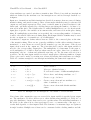
TimeNET 4.0
A Software Tool for the
Performability Evaluation
with Stochastic and Colored Petri Nets
User Manual
Armin Zimmermann and Michael Knoke
Technische Universität Berlin
Real-Time Systems and Robotics Group
Faculty of EE&CS Technical Report 2007-13
ISSN: 1436-9915, August 2007
2
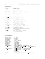
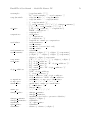
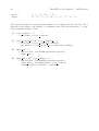
Contents
1 Introduction
1
1.1
History of the Tool . . . . . . . . . . . . . . . . . . . . . . . . . . . . . . . .
1
1.2
Acknowledgments . . . . . . . . . . . . . . . . . . . . . . . . . . . . . . . . .
3
2 TimeNET’s Graphical User Interface
5
2.1
User Interface Genericity and Net Classes
. . . . . . . . . . . . . . . . . . .
6
2.2
Menus . . . . . . . . . . . . . . . . . . . . . . . . . . . . . . . . . . . . . . .
6
2.3
Command Buttons . . . . . . . . . . . . . . . . . . . . . . . . . . . . . . . .
10
2.4
Object Buttons . . . . . . . . . . . . . . . . . . . . . . . . . . . . . . . . . .
11
2.5
Drawing Area . . . . . . . . . . . . . . . . . . . . . . . . . . . . . . . . . . .
12
2.6
File Selection Window . . . . . . . . . . . . . . . . . . . . . . . . . . . . . .
12
2.7
Solution Monitor Windows . . . . . . . . . . . . . . . . . . . . . . . . . . . .
13
2.8
Startup . . . . . . . . . . . . . . . . . . . . . . . . . . . . . . . . . . . . . .
14
3 Extended Deterministic and Stochastic Petri Nets
15
3.1
Supported Model Types . . . . . . . . . . . . . . . . . . . . . . . . . . . . .
16
3.2
Objects and Attributes . . . . . . . . . . . . . . . . . . . . . . . . . . . . . .
17
3.3
Specific Menu Functions . . . . . . . . . . . . . . . . . . . . . . . . . . . . .
20
3.4
Analysis Methods . . . . . . . . . . . . . . . . . . . . . . . . . . . . . . . . .
22
3.5
Evaluation Results . . . . . . . . . . . . . . . . . . . . . . . . . . . . . . . .
30
4 Stochastic Colored Petri Nets
33
4.1
Colored Petri Nets . . . . . . . . . . . . . . . . . . . . . . . . . . . . . . . .
33
4.2
Objects and Attributes . . . . . . . . . . . . . . . . . . . . . . . . . . . . . .
34
4.3
SCPN Expressions . . . . . . . . . . . . . . . . . . . . . . . . . . . . . . . .
41
4.3.1
Constants . . . . . . . . . . . . . . . . . . . . . . . . . . . . . . . . .
41
4.3.2
Functions . . . . . . . . . . . . . . . . . . . . . . . . . . . . . . . . .
42
i
ii
Contents
4.3.3
Place References . . . . . . . . . . . . . . . . . . . . . . . . . . . . .
42
4.3.4
Definition and Measure References . . . . . . . . . . . . . . . . . . .
42
4.3.5
Token and Attribute References . . . . . . . . . . . . . . . . . . . . .
43
4.3.6
Operators . . . . . . . . . . . . . . . . . . . . . . . . . . . . . . . . .
43
4.3.7
Basic Data Types . . . . . . . . . . . . . . . . . . . . . . . . . . . . .
43
4.3.8
Structured Types . . . . . . . . . . . . . . . . . . . . . . . . . . . . .
44
4.3.9
Value Parameters . . . . . . . . . . . . . . . . . . . . . . . . . . . . .
45
4.4
Specific Menu Functions . . . . . . . . . . . . . . . . . . . . . . . . . . . . .
45
4.5
Simulation . . . . . . . . . . . . . . . . . . . . . . . . . . . . . . . . . . . . .
49
4.6
Result Monitor . . . . . . . . . . . . . . . . . . . . . . . . . . . . . . . . . .
52
4.7
Manual Transitions . . . . . . . . . . . . . . . . . . . . . . . . . . . . . . . .
58
4.8
Parametrizable Module Concept . . . . . . . . . . . . . . . . . . . . . . . . .
60
4.8.1
Modules . . . . . . . . . . . . . . . . . . . . . . . . . . . . . . . . . .
60
4.8.2
Module Implementation . . . . . . . . . . . . . . . . . . . . . . . . .
60
4.8.3
Module Instantiation . . . . . . . . . . . . . . . . . . . . . . . . . . .
61
TimeNET Scripting Engine . . . . . . . . . . . . . . . . . . . . . . . . . . .
61
4.9.1
Creating Javascript scripts . . . . . . . . . . . . . . . . . . . . . . . .
62
4.9.2
Integration of external data . . . . . . . . . . . . . . . . . . . . . . .
64
4.10 SCPN Simulation - System Architecture . . . . . . . . . . . . . . . . . . . .
66
4.11 Database Access
67
4.9
. . . . . . . . . . . . . . . . . . . . . . . . . . . . . . . . .
5 Technical Notes
69
5.1
System Requirements . . . . . . . . . . . . . . . . . . . . . . . . . . . . . . .
69
5.2
Downloading TimeNET . . . . . . . . . . . . . . . . . . . . . . . . . . . . .
69
5.3
How to Install the Tool . . . . . . . . . . . . . . . . . . . . . . . . . . . . . .
70
5.4
Configure a multi-user installation . . . . . . . . . . . . . . . . . . . . . . . .
70
5.5
Starting the Tool . . . . . . . . . . . . . . . . . . . . . . . . . . . . . . . . .
70
5.6
Configuring the User Interface . . . . . . . . . . . . . . . . . . . . . . . . . .
71
5.7
Upgrading to TimeNET 4.0 . . . . . . . . . . . . . . . . . . . . . . . . . . .
71
5.7.1
71
Conversion of old Model Files . . . . . . . . . . . . . . . . . . . . . .
A Model File Format .XML
73
B Model File Format .TN
75
Contents
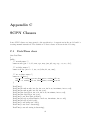
C SCPN Classes
iii
81
C.1 DateTime class . . . . . . . . . . . . . . . . . . . . . . . . . . . . . . . . . .
81
C.2 Delay class . . . . . . . . . . . . . . . . . . . . . . . . . . . . . . . . . . . . .
84
D Javascript Classes
85
D.1 JavaScript-API . . . . . . . . . . . . . . . . . . . . . . . . . . . . . . . . . .
85
D.2 XPath Syntax . . . . . . . . . . . . . . . . . . . . . . . . . . . . . . . . . . .
93
References
96
iv
Contents
Chapter 1
Introduction
This manual describes the software package TimeNET (version 4), a graphical and interactive toolkit for modeling with stochastic Petri nets (SPNs) and stochastic colored Petri
nets (SCPNs). TimeNET has been developed at the Real-Time Systems and Robotics
group of Technische Universität Berlin, Germany (http://pdv.cs.tu-berlin.de/). The
project has been motivated by the need for powerful software for the efficient evaluation
of timed Petri nets with arbitrary firing delays. TimeNET and its predecessor DSPNexpress were influenced by experiences with other well-known Petri net tools, e.g., GreatSPN
and SPNP. For the latest information about TimeNET, check the tool’s home page at
http://pdv.cs.tu-berlin.de/~timenet/.
The manual describes the features and usage of the tool. The aim is to help the user to work
with the tool without going into the details of its components. Additional publications are
available which describe in particular the implemented evaluation techniques including their
mathematical background. References are given in this manual. These papers are available
upon request from the authors, or can be downloaded from their home pages.
Parts of this text are based on the TimeNET 3.0 [21] and TimeNET 2.0 manuals [14] as
well as other material about TimeNET. An overview of older versions of the tool is given
in references [8, 23, 18], while the current version has been announced in [20]. Background
information about stochastic discrete event systems as well as a range of applications can be
found in [22].
1.1
History of the Tool
The software package DSPNexpress [15] has been developed at the Technische Universität
Berlin since 1991, mainly influenced by the tool GreatSPN, and has been maintained at the
Universities of Dortmund and Leipzig later. It provides a user-friendly graphical interface
running under X11 and is especially tailored to the steady-state analysis of deterministic and
stochastic Petri nets. For the class of generalized and stochastic Petri nets, steady-state and
transient analysis components are available. A refined numerical solution algorithm is used
for steady-state evaluation of DSPNs, facilitating parallel computation of intermediate results. Isolated components and isomorphisms of subordinated Markov chains of deterministic
transitions are detected and exploited.
1
2
TimeNET 4.0 User Manual — Introduction
The first version of TimeNET was a major revision of DSPNexpress at TU Berlin. It contained all analysis components of the latter at that time, but supported the specification
and evaluation of extended deterministic and stochastic Petri nets (eDSPNs). Expolynomially distributed firing delays are allowed for transitions. Different solution algorithms can be
used, depending on the net class. If the transitions with non-exponentially distributed firing
delays are mutually exclusive, TimeNET can compute the steady-state solution. DSPNs with
more than one enabled deterministic transition in a marking are called concurrent DSPNs.
TimeNET provides an approximate analysis technique for this class. If the mentioned restrictions are violated or the reachability graph is too complex for a model, an efficient
simulation component is available in the TimeNET tool. A master/slave concept with parallel replications and techniques for monitoring the statistical accuracy as well as reducing
the simulation length in the case of rare events are applied. Analysis, approximation, and
simulation can be performed for the same model classes. TimeNET therefore provides a unified framework for modeling and performance evaluation of non-Markovian stochastic Petri
nets.
Enhancements of TimeNET 3.0 [23, 19, 21] included
• an algorithm for the transient analysis of DSPNs
• a component for the steady-state and transient analysis of discrete time deterministic
and stochastic Petri nets
• a component especially designed for manufacturing systems, including
– modeling with hierarchically and colored stochastic Petri nets
– independent models for structure and work plans
– steady-state analysis and simulation
– model based control
• a completely rewritten graphical user interface (Agnes), which integrates all different
net classes and analysis algorithms
The new version TimeNET 4.0 (stable version available since 2007) includes a completely
rewritten JAVA graphical user interface and provides support of the Microsoft Windows
operating system [20]. It supports a new class of stochastic colored Petri nets (SCPNs). A
standard discrete-event simulation has been implemented for the performance evaluation of
SCPN models. SCPNs allow arbitrary distributions of firing delays including zero delays,
complex token types, global guards, time guards, and marking dependent transition priorities. Petri net classes are defined by an extendable XML schema in TimeNET 4.0 which
affects the behavior of the graphical user interface. A model is a well-formed XML document
which is validated automatically.
Recent enhancements of TimeNET 4.0 include
• a generic graphical user interface in JAVA based on an XML net class representation,
easily extendable for most graph-like modeling formalisms
TimeNET 4.0 User Manual — Introduction
3
• user interface and evaluation algorithms run under Windows and Linux operating
system environments
• modeling and simulation of stochastic colored Petri nets
• graphical display of SCPN simulation results
• independent components for modeling, simulation, analysis, and result output allowing
the GUI to be run on a different computer than the analysis modules
1.2
Acknowledgments
The TimeNET developers are thankful for the contributions of the numerous master students, project programmers, and Ph. D. students of the Real-Time Systems and Robotics
Group at TU Berlin. Without them, the development and implementation of TimeNET 4.0
and earlier versions would not have been possible:
Tobias Bading, Enrik Baumann, Frank Bayer, Mario Beck, Heiko Bergmann, Stefan Bode,
Knut Dalkowski, Renate Dornbrach, Patrick Drescher, Heiko Feldker, Jörn Freiheit, Magdalena Gajewsky, Reinhard German, Armin Heindl, Matthias Hoffmann, Alexander Huck,
Frank Jakop, Christian Kelling, Oliver Klössing, Kolja Koischwitz, Felix Kühling, Thomas
Kuhlmann, Andreas Kühnel, Christoph Lindemann, Christian Lühe, Samar Maamoum,
Markolf Maczek, Ronald Markworth, Rasoul Mirkheshti, Jörg Mitzlaff, Martin Müller, Maud
Olbrisch, Daniel Opitz, Daniel Pirch, Markus Pritsch, Ralf Putz, Dawid Rasinski, Oliver Rehfeld, Stefan Rönisch, Jens-Peter Rotermund, Ken Schwiersch, Anja Seibt, Jan Trowitzsch
Dietmar Tutsch, Frank Ulbricht, Matthias Weiß, Florian Wolf, Katinka Wolter, Henning
Ziegler, Robert Zijal, Andrea Zisowsky.
Moreover, the financial support of the German Research Council (DFG) and various industrial project partners is gratefully acknowledged. The extension for colored models has been
carried out during a project funded by General Motors Research and Development.
4
TimeNET 4.0 User Manual — Graphical User Interface
Chapter 2
TimeNET’s Graphical User Interface
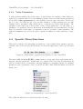
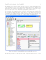
A powerful and easy-to-use graphical interface is an important requirement during the process of modeling and evaluating a system. For version 4.0 of TimeNET a new platformindependent, generic graphical user interface based on Java has been implemented. The
subsequent Section 2.1 explains the underlying concept of net classes and its consequences
for the user interaction. All currently available and future extensions of model types and
their corresponding analysis algorithms are integrated with the same “look-and-feel” for the
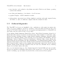
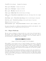
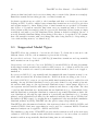
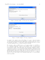
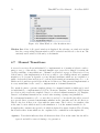
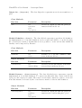
user. Figure 2.1 shows a sample screen shot of the interface.
Figure 2.1: Graphical user interface of TimeNET 4.0
The window is composed of four main areas: a menu bar (top) with an icon bar below,
drawing area (left), attribute area (right), and a net class-specific modeling tool bar (bottom).
5
6
TimeNET 4.0 User Manual — Graphical User Interface
The upper row of the window contains some menus with commands for file handling, editing,
and other model specific commands and is explained in Section 2.2 below. Frequently used
commands are available in the upper tool bar. Their use is explained in Section 2.3. A toolbar
at the bottom of the main windows contains model elements that are available for the current
model type. Section 2.4 explains these object buttons in general, while the actual elements
depend on the current net class and are explained in the corresponding section. Finally, use
of the main drawing area and attribute area is covered by Section 2.5.
2.1
User Interface Genericity and Net Classes
The graphical user interface for TimeNET 4.0 has been completely rewritten in JAVA, and
can therefore be run in both Unix- and Windows-based environments. The new GUI retains
the advantages of the former one (Agnes — A generic net editing system), especially in
being generic in the sense that any graph-like modeling formalism can be easily integrated
without much programming effort. Nodes can be hierarchically refined by corresponding
submodels. The GUI is thus not restricted to Petri nets, and is already being used for other
tools than TimeNET. As a stand-alone program it is named PENG, which is short for
platform-independent editor for net graphs.
Two design concepts have been included in the interface to make it applicable for different
model classes: A net class corresponds to a model type and is defined by a XML schema file.
Node objects, connectors and miscellaneous others are possible elements which are defined
by a basic XML schema which can be extended in each net class. For each node and arc
type of the model the corresponding attributes and the graphical appearance is specified.
The shape of each node and arc is defined using a set of primitives, and may depend on
attribute values of the object. Actual models are stored in an XML file consistent with the
model class definition.
Program modules can be added to the tool to implement model-specific algorithms. A module
can select its applicable net classes and extend the menu structure by adding new algorithms.
All currently available and future extensions of net classes and their corresponding analysis
algorithms are thus integrated with the same ”look-and-feel” for the user. Figure 2.1 shows
a sample screen shot of the GUI displaying an eDSPN net class.
Depending on the net class, different objects are available in the upper and lower icon
lists. In addition to that, analysis methods typically are applicable for one net class only.
Those methods are integrated in the menu structure of the tool, which therefore changes
automatically if a different net class is opened. There are standard menus with the necessary
editing commands in the top row. Commands should be self-explanatory and follow usual
GUI-style.
2.2
Menus
The following section describes the commands that are available in the main menu independent of the current net class. Additional features for certain net classes are explained later in
TimeNET 4.0 User Manual — Graphical User Interface
7
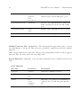
the corresponding sections. Figure 2.2 shows the menu region of the graphical user interface
with the minimal set of menus.
Figure 2.2: Menu region of the graphical user interface
The menu entries can be accessed by clicking with the left mouse button, or by pressing
Alt and the key that is underlined in the name of the menu entry. This is also valid for
all submenus. To leave a submenu that has been opened with keystrokes, press Esc . Some
commands can be accessed directly by control key combinations, as shown in the menus
beside the command. If applicable, this is mentioned in the menu entry explanation. An
existing model file can e.g. be opened by pressing Ctrl-O (c.f. Figure 2.3) without opening
the menu. As usual, menu entries that are not available at the moment due to the state
of the interface or the selected object, are shown in gray and cannot be activated. A short
description of a menu entry is shown in a tooltip after some time if the mouse pointer is over
the entry.
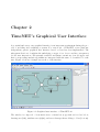
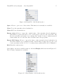
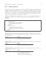
Figure 2.3: Menu File
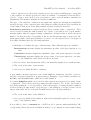
Figure 2.3 shows the menu structure for entry File. Please remember that there might be
additional menu entries available, depending on the current net class. These entries are
explained in the net class-specific section of this manual. The following commands are the
default:
New... After selecting a net class from the upcoming selection window, a new model editor
window for models of this class is opened. The drawing area is initially empty and
the new model is called Untitled.xml until it is given a name with Save as.... The
available set of net classes depends on the net class description files that are currently
accessible for the user interface. The New... command can directly be invoked by
pressing Ctrl-N .
Open... From the subsequent file selection menu (explained in Section 2.6) the model to
be opened can be selected. A new window of the editor is opened with the model
afterward. The extension .xml for the standard TimeNET 4.0 file format is set initially,
8
TimeNET 4.0 User Manual — Graphical User Interface
but it can be changed as desired. The tool is also able to open models in the old .TNformat, which makes it possible to import models from older versions of TimeNET.
The Open... command can directly be invoked by pressing Ctrl-O .
Open Recent File A list of recently opened model files is displayed. One of these models
can be opened by selecting its name. If the GUI is started for the first time, the list is
empty.
Save Save changes of the current net under the model name that is shown in the title bar
of the editor window. If in front of the net path (located in the title bar) an asterisk
(∗) is shown, the current net has been changed since the last Save. Ctrl-S also saves
the net.
Save as... Save the current model under a new name, which has to be selected in a subsequent file selector window. The model is saved in the standard TimeNET 4.0 .xml
format.
Print/Export Image Exports the current figure to a drawing program Batik, from which
it is possible to print, edit and save the picture. The exported file type is Scalable Vector Graphics (SVG) which is an XML markup language for describing two-dimensional
vector graphics and is supported by an increasing number of open source and commercial tools. Because this module is directly based on the shape definitions contained in
the net class definitions, it will work also for future net classes. Only the currently
shown model page is exported for a hierarchical model. The menu entry opens a file
selection window which allows to specify the desired filename.
Settings Opens a settings window where some options of the GUI can be configured. This
includes paths, fonts, colors, default simulation values as well as various other parameter.
Exit Closes all editor windows and quits the user interface. If there are unsaved changes in
any one of the open windows, it is possible to cancel the command. Keyboard access:
Alt-Q .
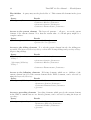
Figure 2.4: Menu Edit
Figure 2.4 shows the menu Edit with the following commands:
Undo: <command> Takes back the last change in the drawing area. All recent changes
are stored and can be rolled back one after another. The last change (command) which
TimeNET 4.0 User Manual — Graphical User Interface
9
can be taken back by applying Undo is shown on the right side of the Undo menu
entry. Keyboard shortcut: Ctrl-Z .
Cut Copies the selected model objects into the internal buffer and deletes them from the
model. For a description of selecting objects and other operations on model elements,
refer to Section 2.5. Keyboard shortcut: Ctrl-X .
Copy Copies the selected model objects into the internal buffer. For a description of selecting
objects and other operations on model elements, refer to Section 2.5. Alternative:
Ctrl-C .
Paste Adds the model elements from the internal buffer to the current model. The elements
are added in a position slightly away from the position of the copied/cut elements. They
are still selected after the paste operation, and can therefore easily be moved to the
desired position. Pasting can also be done by pressing Ctrl-V .
Copying and pasting is also possible between different pages of a hierarchical model,
and between open windows containing different nets. However, it is of course impossible
to paste net objects into an incompatible model (belonging to another net class). In
net classes where object names have to be unique, Paste renames the added objects
automatically.
Hide Output Hides any output of the simulation windows if this entry is selected.
Figure 2.5: Menu View
Menu View (shown in Figure 2.5) contains operations on the currently selected model view:
Create new view on file Creates a new editor window with a copy of the model which can
be selected by the shown file list. In Figure 2.5 is only one model opened, such that the
file list contains only this model name as an entry (C:\Models\EDSPN\mmppd13.xml).
Grid activation If this entry is selected, it activates an invisible grid for aligning objects.
New objects are automatically aligned on the grid. Already drawn objects are kept in
their current positions, but are aligned on the grid when being moved.
Sharp edges If this entry is selected, arcs have sharp edges. Otherwise they have rounded
edges.
10
TimeNET 4.0 User Manual — Graphical User Interface
Scale down Image Each click scales down the image by 10 percent (zoom out), resulting
in more space on the drawing area to add objects.
Scale up Image Scales up the image by 10 percent (zoom in) per click.
Scale to normal size Sets the size of the image back to the original size which is defined
by the GUI.
Close Closes the current model view which is the currently active window.
Close all views Closes all views of the current model.
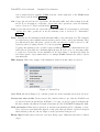
Figure 2.6: Menu Window
Figure 2.6 shows the Window menu contents:
Cascade Stacks all opened model views so that each window title bar is visible.
Tile Displays all opened model views side by side, so that all windows are visible at once.
The size of the windows is decreased but the model inside each window is not scaled
down.
<Models> This is a list of currently available model views. By selecting one model in this
list, the corresponding view is selected and moved to the front of all other windows.
2.3
Command Buttons
On the top of the main window right below the menu bar, a button area (toolbar) with some
of the most frequently used menu commands is available. Each button is depicted as an icon.
A short description is shown in a tooltip after some time if the mouse pointer is over an icon.
The command buttons are shown in Figure 2.7, and each of them can be either activated or
disabled depending on the user interface state, e.g. Copy can only be started when an object
in the drawing area is selected.
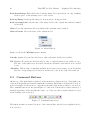
Figure 2.7: Command button area
The functions that are started by most of the buttons have already been explained in Section 2.2 before.
TimeNET 4.0 User Manual — Graphical User Interface
11
New equal to File/New...: Creates a new model
Open equal to File/Open...: Opens a model file
Save equal to File/Save: Saves the active model
Undo equal to Edit/Undo: Takes back the last model change
100% equal to View/Scale to normal size: Sets the size of the image back to the original
size
Scale Down equal to View/Scale down Image: Scales down the image by 10 percent
Scale Up equal to View/Scale up Image: Scales up the image by 10 percent
Delete Deletes the selected objects
Grid Activation equal to View/Grid activation: Activates a grid for aligning objects
In some net classes there are additional command buttons available at the right side of the
default buttons. They are explained in the net class sections.
2.4
Object Buttons
The net objects are displayed on buttons in the area on the bottom of the main window.
The available objects completely depend on the current net class. Please refer to the net
class specific sections of this document for an explanation of the object semantics. Figure 2.8
shows the buttons for the EDSPN class as an example.
Figure 2.8: Object button example for net class EDSPN
Each available object is shown as an icon. A short description is shown in a tooltip after
some time if the mouse pointer is over an icon. There are several types of objects available in
general, which correspond to the nodes, arcs and definitions of the model class. Clicking an
icon allows to add objects of this type. From then on, the corresponding element is created
every time the left mouse button is pressed in the drawing area (see next section), until a
different selection is made.
The leftmost object button which is shown in Figure 2.9 switches back to the default selection
mode which allows to select and edit objects in the drawing area. In this mode it is also
possible to select multiple objects (e.g. for copying these objects to the clipboard) by clicking
and dragging the mouse in the drawing area. Obviously this button is available independently
of the current net class.
12
TimeNET 4.0 User Manual — Graphical User Interface
Figure 2.9: Generic button to activate selection mode
2.5
Drawing Area
The main drawing area covers the biggest portion of the user interface (see Figure 2.1), and
displays a part of the current model. The shown model can be edited with the left mouse
button like using a standard drawing tool with operations for selecting, moving, and others.
Editing is only possible in selection mode which is described on page 11. In all other modes,
the corresponding object is created with the left mouse button.
Arcs can be created by selecting the source object and dragging the mouse to the target
object. While dragging, the target object will be selected if this target is allowed by the
underlying net class, e.g. drawing an arc from a transition to another transition is not possible
in a Petri net and the target transition will not be selected. Arcs are initially created as a
direct line between the source and destination objects. Intermediate points can be added by
double-clicking with the left mouse button on the arc, where the additional point of the arc
should be positioned. Intermediate points can be dragged to other positions to change the
arc’s appearance.
Clicking on an empty area and dragging with the mouse selects all objects inside the drawn
rectangle. Clicking on a selected object and dragging it, moves all selected objects. For
commands like copy and delete the current selection is used. Clicking and dragging an end
point of an arc can be used to change the source or destination object of the arc. In the same
manner it is possible to move intermediate points of arcs or visible attributes of objects like
the name. The position of those attributes is relative to their main object. Therefore, if only
the name of a transition is moved, it stays in the same relative position to the transition
when the transition is moved afterward.
If an object has been selected, its attributes and their current values, e.g. for a place the
initial marking and the name are displayed in the attribute window on the right side of the
drawing area. Attributes are defined by the net class for each object type individually. New
objects are created with initial default values for all attributes which are also defined in the
net class.
If an object is hierarchically refined (like a substitution transition), double-clicking it switches
the drawing area view to the refining model (sub page).
Selecting an object with the right mouse button opens a popup menu with object-specific
actions as shown in Figure 2.10. These actions mostly involve a delete and rotate action.
2.6
File Selection Window
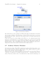
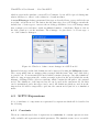
For several commands a file needs to be selected by the user, e.g. when opening or saving
a model to disk. Figure 2.11 shows the corresponding window which is a typical Java file
selection dialog.
TimeNET 4.0 User Manual — Graphical User Interface
13
Figure 2.10: Popup Menu
Figure 2.11: File Selection Window
The current directory can be changed by clicking in the upper text field where the current
directory name is displayed. The files that are contained in the current directory are shown
in the file list in the center of this dialog. The file type in the bottom part restricts the files
that are shown.
A file can be selected by double-clicking it in the Files box, or by entering its name in the
Selection box. The initial directory from which model files can be selected is set by the GUI
(usually the path of the most recently loaded model). When working with model files, the
standard extension .xml for TimeNET 4.0 file format models is initially set, but it can be
changed if necessary. Cancel exits from the file selection without action.
2.7
Solution Monitor Windows
Most analysis algorithms of TimeNET are implemented as independent background processes
that are started by the user interface when necessary. Their output is visible in a solution
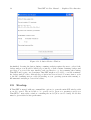
monitor window like the one shown in Figure 2.12.
Thus the progress of the analysis algorithms as well as possible errors are shown. The successful end of an analysis process usually means that the text ...Finished is printed in the
window. The monitor window can be closed with the Close button after the analysis process
14
TimeNET 4.0 User Manual — Graphical User Interface
Figure 2.12: Solution Monitor Window
has finished. Pressing the button during a running analysis requires the user to select if the
background process should be killed (stop solution) or shall continue. Running background
processes do not need the user interface and can therefore e.g. keep running after exiting
TimeNET and logging out. Sometimes TimeNET might not be able to correctly terminate
the background processes, although Stop solution has been selected. You may want to refer
to the list of running user processes (depending on your operating system environment), to
kill unwanted analysis processes if necessary.
2.8
Startup
If TimeNET is started without command-line options, it opens the main GUI window with
no model opened. The model file to be opened can be given as a parameter and forces
TimeNET to start with a window containing the model (if it can be found). Model files
must be given with absolute path names.
Chapter 3
Extended Deterministic and
Stochastic Petri Nets
This section covers the use of the TimeNET tool in the domain of (non-colored) stochastic
Petri nets, specifically with non-exponentially distributed firing times. The net class called
EDSPN in TimeNET should not be taken as a mathematical definition of extended deterministic and stochastic Petri nets. It should rather be understood as a model class containing the
modeling power of several well-known subclasses like GSPNs, DSPNs and eDSPNs having
either an underlying continuous or discrete time scale. In fact, sometimes the same model
is understood differently depending on the analysis algorithms that interpret the model
specifically. Please refer to subsection 3.1 for a description of supported model types.
The model objects (places, transitions, arcs, textual elements) available in the net class
EDSPN are explained in detail in Section 3.2. EDSPN-specific features of the graphical user
interface and available analysis algorithms are covered by Sections 3.3 and 3.4.
In the following it is assumed that the reader is familiar with the elementary Petri net
concepts; a comprehensive survey can be found in [16], for instance.
TimeNET uses the customary Petri net formalism as e.g. in [1, 2]. A SPN consists of places
and transitions, which are connected by input, output, and inhibitor arcs. In the graphical
representation, places are drawn as circles, transitions are drawn as thin bars or as rectangles, and arcs are drawn as arrows (inhibitor arcs end with a small circle, connected with
transitions). Places may contain indistinguishable tokens, which are drawn as black dots.
The vector containing the number of tokens in each place is the state of the SPN and is
referred to as marking. A marking-dependent multiplicity can be associated with each arc.
Places that are connected with a transition by an arc are referred to as input, output, and
inhibitor places of the transition, depending on the type of the arc. A transition is said to be
enabled in a marking if each input place contains at least as many tokens as the multiplicity
of the input arc and if each inhibitor place contains less tokens than the multiplicity of the
inhibitor arc. A transition fires by removing tokens from the input places and adding tokens
to the output places according to the multiplicities of the corresponding arcs, thus changing
the marking. The reachability graph is defined by the set of vertices corresponding to the
markings reachable from the initial marking and the set of edges corresponding to the transition firings. The transitions can be divided into immediate transitions firing without delay
15
16
TimeNET 4.0 User Manual — Net Class EDSPN
(drawn as thin bars) and timed transitions firing after a certain delay (drawn as rectangles).
Immediate transitions have firing priority over timed transitions.
Stochastic specifications are added to the formalism such that a stochastic process is underlying an SPN. Possible conflicts between immediate transitions are resolved by priorities
and weights assigned to them. Firing delays of timed transitions are specified by deterministic delays or by random variables. Important cases are transitions with a deterministic
delay (drawn as filled rectangles), with an exponentially distributed delay (drawn as empty
rectangles), and with a generally distributed delay (drawn as dashed rectangles). In case of
non-exponentially distributed firing delays, firing policies have to be specified [2]. We assume
that each transition restarts with a new firing time after being disabled, corresponding to
“race with enabling memory” as defined in [2].
3.1
Supported Model Types
TimeNET allows the evaluation of several model classes. To clarify the notations for the
different classes of SPNs, a short summary is given in the following.
In generalized stochastic Petri nets (GSPNs) [4] immediate transitions and exponentially
timed transitions can be specified.
Deterministic and stochastic Petri nets (DSPNs) [3] extend GSPNs by allowing deterministically timed transitions under the restriction that at most one of them is enabled in each
marking. The restriction is caused by the numerical analysis method, but does not apply to
simulation.
In concurrent DSPNs [6], exponentially and deterministically timed transitions may be enabled without restrictions. It is thus identical to DSPNs from the modeling point of view.
In extended DSPNs [6], at most one expolynomially timed transition may be enabled in each
marking. An expolynomial distribution can be piecewise defined by exponential polynomials and has finite support. An expolynomial distribution may contain jumps, therefore it
can represent random variables with mixed continuous and discrete components. The class
of expolynomial distributions contains many known distributions (e.g., deterministic delay,
uniform distribution, triangular distribution, truncated exponential distribution, finite discrete distribution), allowing the approximation of practically any distribution (e.g., by using
splines), and is particularly well suited for the numerical analysis. Since the probability density function (PDF) seems to be graphically more significant for the user than the cumulative
distribution function (CDF), TimeNET uses the pdf for temporal specifications.
TimeNET provides the numerical analysis of the stationary behavior for GSPNs, DSPNs, and
extended DSPNs. Stationary approximation can be used for concurrent DSPNs. Transient
numerical analysis can be applied to GSPNs and DSPNs.
The simulation component of TimeNET can perform the transient as well as the stationary
evaluation of SPNs in continuous time without the restriction of not more than one enabled
transition with non-exponentially distributed firing time in each marking.
TimeNET 4.0 User Manual — Net Class EDSPN
3.2
17
Objects and Attributes
This section lists and explains all available modeling objects in the EDSPN net class. As
stated before, not all of them can be used in any combination depending on the analysis
algorithm that should be applied to the model.
Figure 3.1: Model element buttons for net class eDSPN
Figure 3.1 shows the model element button area for net class EDSPN in its initial state.
They are explained in the following with their attributes.
Places are depicted as circles.
• The text of a place is an identification string which is shown as a label nearby the place
in the model. When a place is created, it gets an initial name P plus a number. All
names of model elements must be unique.
• The initial marking of a place is a text, either specifying a natural number or containing
the name of a marking parameter with the initial token number. Places have an initial
marking of zero.
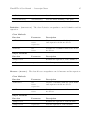
Transitions are either exponential, deterministic, immediate, or general transitions. The text
of each transition is an identification string and shown as a label. When a transition is
created, it gets an initial name ”T” plus a number.
Exponential transitions are drawn as empty rectangles.
• Their firing delay is exponentially distributed. Its default value (i.e., the expectation
of the exponentially distributed firing time) is 1. Please be aware that for consistency
reasons, transition firing times are specified as delays for all transition types. Firing
rates of exponential transitions have to be transformed into a delay by taking their
reciprocal value.
• The serverType is either ”Infinite Server” or ”Single Server” (default value). It determines the way in which multiple customers are handled. Informally speaking, transitions with infinite server semantics can be enabled concurrently to themselves as
many times as there are enough input token sets available. This server characteristic is known from queuing theory. In case of a single server type the firing times are
determined sequentially.
Immediate transitions are drawn as thin bars.
• The priority is a natural number (default: 1), that defines a precedence among simultaneously enabled immediate transition firings. The default priority is 1, higher numbers
mean higher priority.
18
TimeNET 4.0 User Manual — Net Class EDSPN
• The weight is a real value (default: 1), specifying the relative firing probability of the
transition with respect to other simultaneously enabled immediate transitions that are
in conflict.
• The enablingFunction (also called guard) is a marking-dependent expression1 , which
must be true in order to allow the transition to be enabled. Its default empty state
means that the transition is allowed to fire.
Deterministic transitions are drawn as black filled rectangles.
• The fixed firing delay of this transition type is initially 1.
General transitions are depicted as rectangles, filled with gray.
• The firing delay of a general transition is described by its probability mass function,
and belongs to the class of expolynomial functions. Such a distribution function can
be piecewise defined by exponential polynomials and has finite support. It can contain
jumps, making it possible to mix discrete and continuous components. Many known
distributions (uniform, triangular, truncated exponential, finite discrete) belong to this
class. The default firing delay UNIFORM(0.0,1.0); of general transitions is uniformly
distributed in the interval zero to one. The full available syntax definition can be found
at page 78 under the term <pmf definition>.
An Arc is depicted as an arrow. To create an arc, select the source with the left mouse button,
and drag the mouse with the button still pressed over the destination object. Forbidden
arcs disappear after releasing the button (e.g. arcs between transitions are not allowed).
While dragging the mouse over a destination object, a valid destination is shown when the
destination object changes into the selected state (changes the color). To add an intermediate
point, double click on the arc at the desired position for this intermediate point. A point is
added at this position and can be moved to change the arc position.
• The arc multiplicity text is 1 initially, but can be changed by selecting the arc and
enter a different value in the attribute window. This value can be marking-dependent
– an arc going from a place P1 to a transition with multiplicity #P1 would flush all
tokens from the place when the transition fires.
Inhibitor arcs are depicted by a line with a small circle on one end. These type of arcs
always go from a place to a transition.
• The inhibitor arc condition text is 1 initially, but can be changed by selecting the arc
and enter a different value in the attribute window. The meaning of an inhibitor arc
is that if the place has at least the number of tokens specified by the condition it will
hinder the transition from firing, i.e., opposite to that of a normal arc.
1
For example, #P3=1 is true if the number of tokens in place P3 is equal to 1. For a complete syntax
definition of marking dependent expressions, refer to the Appendix at page 78.
TimeNET 4.0 User Manual — Net Class EDSPN
19
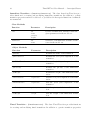
Performance measures are depicted in the model by a string ”name = expression” or
if the expression has been already evaluated the string changes to ”name = value”. They
can be created by using the button named ”R=” in the object button area. A performance
measure defines what is computed during an analysis. A typical value would be the mean
number of tokens in a place. Depending on the model, this measure may correspond to the
mean queue length of customers waiting for a service or to the expected level of work pieces
in a buffer. Measures have the following attributes:
• The name of the measure.
• An expression which should be evaluated.
• The computed result which is changed after a successful evaluation of the model. The
meaning of a computed value may depend on the algorithm that computed it, e.g.
there are different results for a transient and a steady-state evaluation for the same
measures. A result can be cleared by deleting the result value in the attribute window.
For the definition of measures a special grammar is used (see Appendix on page 80). A
performance measure (in the context of the EDSPN net class) is an expression that can
contain numbers, marking and delay parameters, algebraic operators, and the following basic
measures:
• P{ <logic condition> }; corresponds to the probability of <logic condition>
• P{ <logic cond 1> IF <logic cond 2> }; computes the probability of <logic cond 1>
under the precondition of <logic cond 2> (conditional probability)
• E{ <marc func> }; refers to the expected value of the marking-dependent expression
<marc func>
• E{ <marc func> IF <logic condition> }; corresponds to the expected value of the
marking-dependent expression <marc func>; only markings where <logic condition>
evaluates to true are taken into consideration
Marking-dependent functions in performance measure definitions are of the form #Pn, referring to the number of tokens in place Pn. Logic conditions usually contain comparisons of
marking-dependent functions and numbers. Examples of performance measures are E{#P5};
and N/(5*P{#P2<3});.
A constant definition which can be used in marking and delay parameters is depicted as
a string ”name := expression”. They can be created by using the button named ”D=”
in the object button area. After defining N := 5 it is possible to write N in any place or
transition where a number is allowed. But it is important to set the type of the definition
correctly, because an initial marking is an integer value while a transition delay is a real
value. Definitions have the following attributes:
• The defType specifies the data type of a definition and can be ”int” or ”real”.
20
TimeNET 4.0 User Manual — Net Class EDSPN
• The name of the definition.
• An expression which is the definition value and is internally replaced for every occurrence of the definition name.
3.3
Specific Menu Functions
This section describes the miscellaneous functions of the graphical user interface that are
available only for the net class EDSPN. Figure 3.2 shows the appearance of the top level
menu bar. Performance analysis modules (menu entries under Evaluation) are explained in
their own subsequent section.
Figure 3.2: Main menu of graphical user interface for net class EDSPN
The first additional menu Validate contains evaluation functions based on the structure of
the EDSPN model. It is shown in Figure 3.3.
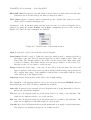
Figure 3.3: Menu Validate for net class EDSPN
The additional functions are described in the following.
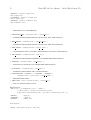
Estimate Statespace Computes an estimation of the number of reachable states that the
current model has, based on the structure of the model. Figure 3.4 shows an example
monitor window with the result output.
Traps Computes the set of minimal traps (i.e. place sets that will never become unmarked
in any subsequent marking after they are once marked). Figure 3.5 shows an example.
Every trap is described by the corresponding places and their initial marking.
Siphons Computes the set of minimal siphons (i.e. place sets that will never become marked
again in any successive marking after they become unmarked). The output of this
command is similar to the one of Traps.
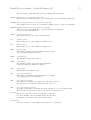
Check Structure Obtains minimal place invariants of the model and extended conflict sets
of immediate transitions, showing them in two windows.
A place invariant (or semi flow ) is informally a set of places for which a weighted sum
of tokens remains the same for any reachable marking of the Petri net. Figure 3.6 shows
TimeNET 4.0 User Manual — Net Class EDSPN
21
Figure 3.4: Result example of a state space size estimation
Figure 3.5: Result example for the trap computation
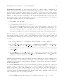
an example of the output for the model in Figure 2.1 on page 5, where the number
of tokens in places HeavyTraffic plus LightTraffic is always 1 (the token count of
the invariant), the number of tokens in places Queue plus QueueAvailable is always
3, and place NewPacket is not contained in any place invariant.
The extended conflict set (ECS) is the second output in Figure 3.6. An ECS is a
set of immediate transitions, obtained by the transitive closure of transitions that
are in structural conflict. This is important for the specification of firing probabilities,
because they are relative to the other transitions in the same ECS. Adjust the priorities
of immediate transitions to put transitions into different ECS, because transitions with
differing priorities cannot be in conflict with each other and will therefore not be in
the same ECS. Check the ECS and adjust the priorities also in the case of confusions,
which are detected and notified by the structural analysis prior to the performance
analysis algorithms.
22
TimeNET 4.0 User Manual — Net Class EDSPN
Figure 3.6: Example of place invariant and extended conflict set results
Tokengame Starts the so called token game of the Petri net model, which is an interactive
simulation of the model behavior. The places shown in the drawing area contain their
respective number of tokens in the current state, and enabled transitions flash. Please
note that the firing times of the transitions are not taken into account. Double-clicking
an enabled transition with the left mouse button causes it to fire, changing the marking
accordingly. This is especially useful for debugging a model, checking whether it works
as it is supposed to. To exit from the token game, select the menu entry again. The
user decides between resetting the marking of the model back to the state before the
token game was started, and keeping the current marking as the new initial marking
before reaching the normal editing mode again.
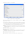
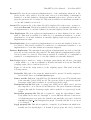
3.4
Analysis Methods
This section explains the performance evaluation functions of TimeNET for the EDSPN net
class. They are all accessible via the Evaluation menu, for which the submenu structure is
shown in Figure 3.7. The different variants of available analysis methods have been organized
systematically, depending on categories like stationary and transient evaluation methods
TimeNET 4.0 User Manual — Net Class EDSPN
23
which are either analysis, approximation, or simulation. Those categories are explained first
to avoid later repetitions.
Figure 3.7: Menu structure of EDSPN performance evaluation algorithms
Transient / Stationary (or Steady-State) A transient evaluation analyzes the model
behavior from the initial marking at time zero until a given end time. Consequently,
it can e.g. for a reliability model be used to answer questions of the type: What is the
probability that after one week of operation, the system is still operable? Or: How many
parts have been produced one hour after a re-setup of a manufacturing system? The
performance measures are computed for the final point in time, but several analysis
algorithms compute and optionally show a figure for the transient evolution of the
measures over time.
Steady-state or stationary evaluation assesses the mean system performance after all
initial transient effects have passed, and a balanced operation mode has been reached.
It is informally comparable to the transient solution for limt→∞ in the normal case.
Steady-state evaluation computes the mean for all performance measures, and can be
used to answer typical questions like: What will be the maximum bandwidth of a communication channel? Or: What will be the expected number of parts in a manufacturing
system’s buffer?
The selection of either transient or steady-state evaluation is done separately for each
evaluation methods in the menu Evaluation. Please note that not for all evaluation
algorithms there are both available.
Analysis / Approximation / Simulation: This selects the basic type of evaluation algorithm. Analysis means a direct and exact numerical performance evaluation with
a full exploration of the reachability graph. Approximation algorithms are also direct
numerical techniques, but try to avoid some of the costly evaluation parts by allowing
some kind of inaccuracy. Simulation algorithms do not compute the reachability graph,
but follow the standard Monte Carlo style simulation approach with some refinements
(details see below). The term evaluation is used throughout this document as a synonym for any of the available performance evaluation algorithms, including all three
types mentioned here.
Miscellaneous remarks for performance evaluations:
24
TimeNET 4.0 User Manual — Net Class EDSPN
Performance measures must be defined to tell the analysis algorithms what to compute. One exception is the stationary analysis, which computes the throughputs
for all timed transitions and the token distribution probabilities for all places.
Performance measures have been explained before (see page 19). The information
on how to get the performance results is given in Section 3.5.
Option windows appear every time the user selects one of the evaluation commands.
The options for every algorithm are explained below and are kept by TimeNET
until the next time the window is opened. The option windows have in common
a set of buttons on the lower part of the window. Start begins the algorithm,
showing the output in a monitor window. Default resets the option values back to
their default. Load and Save can be used to store and retrieve sets of options in an
option file *.opt, while Cancel closes the window without starting the evaluation.
Monitor windows show the output of the evaluation algorithms which are running
as background processes. Please refer to Section 2.7 for details.
Stopping a running evaluation is possible by pressing the Close button of the
monitor window. Sometimes an evaluation method cannot be stopped (especially
on Windows based systems). In this case the running process must be killed
manually by using the task manager on Windows or the kill command on Linux.
The following paragraphs explain the different evaluation algorithms together with their
options, in the sequence as they appear in the Evaluation menu structure (Figure 3.7).
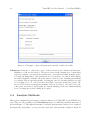
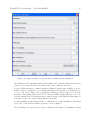
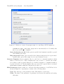
Stationary Analysis computes the steady-state solution of the model with continuous
time. Background information about this algorithm can be found in [9, 6, 7].
Figure 3.8 shows the available options. The Overall solution method defines how the
embedded Markov chain (EMC) is treated during the algorithm: normally, it is explicitly computed and stored (option EMC explicit). It is possible to avoid fill-ins in the
EMC matrix (option fill-in avoidance). Independent parts of the subordinated Markov
chains (SMC) can be computed sequentially or in parallel on a cluster of workstations
(option Computation of SMCs: sequential / distributed). The overall precision is given
as an error value, and the maximum allowed number of iterations for the analysis
algorithm as an integer.
For the integration of matrix exponentials an arithmetic with arbitrary precision can be
used (option Precision of arithmetics: arbitrary / double). The number of bits to store
values can be specified in the case of arbitrary precision (option Bits for arbitrary
precision), and the corresponding truncation error can be given (option Truncation
error ). If the EMC is computed explicitly, the obtained linear system of equations
can either be solved directly or iteratively. For the fill-in avoidance method the initial
iteration vector can either be uniformly distributed, random, or loaded from a file. To
load the vector, one must have been saved during a previous analysis (last option). For
the random initialization of the initial vector a seed value for the used random number
generator can be given.
Please note that in every reachable marking of the model at most one timed nonexponential transition can be enabled. Otherwise the algorithm stops with an error
message. Furthermore, no dead markings are allowed in a steady-state solution.
TimeNET 4.0 User Manual — Net Class EDSPN
25
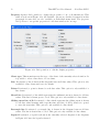
Figure 3.8: Option window for steady state continuous time analysis
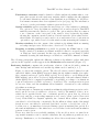
The Experiment option allows to run multiple analysis runs automatically with a given
range of parameter values. Starting the analysis as an experiment opens another dialog
window as shown in Figure 3.9 to define the parameter range and additional experiment
options.
Varying Parameter identifies the name of a definition in the model (explained on
page 19) whose values will be iterated.
From value specifies the start value for the varying parameter of this experiment.
To value specifies the stop value for the varying parameter of this experiment.
Step size allows to define a linear or logarithmic step size. In the linear mode the
26
TimeNET 4.0 User Manual — Net Class EDSPN
Summand is added in each step whereas in the logarithmic mode the Exponent is
multiplied.
Summand (linear) or Exponent (logarithmic) The value which is added or multiplied in each step.
The results of an experiment are written to a file <modelname>.EXPRESULTS which
is located in the model directory as described later in Section 3.5.
Figure 3.9: Option window for simulation/analysis experiment
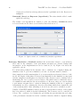
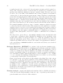
Stationary Simulation / Standard simulates the steady-state behavior of an arbitrary
SPN, and for the estimates of the performance measures are derived. Background
information on the implementation can be found in [13, 12]. Figure 3.10 shows the
applicable options.
For all measures defined in the measure editor, estimates are computed during the
simulation run. To perform a simulation, at least one measure must be defined.
Since samples from the transient phase do not represent the steady-state behavior of the
model, the length of this phase is detected automatically by the simulation component
and the samples from this phase are discarded. The detection can be switched off by
unchecking the detect initial transient button. The initial and recommended choice
are simulation runs with the detection switched on. However, there are cases in which
a performance measure has no variation during the simulation (like in a completely
deterministic model), confusing the detection algorithm, which never signals the end
of the transient phase. After switching it off, those models can be evaluated as well.
Usually a TimeNET simulation run stops after a user-specified accuracy of the results
has been achieved, which is checked statistically. The accuracy can be controlled as
follows. The confidence level defines the probability (in percent) that the real value
of the performance measure lies in the confidence interval, which is computed during
TimeNET 4.0 User Manual — Net Class EDSPN
27
Figure 3.10: Option window for steady-state continuous time simulation
the simulation. The maximum relative half width of the confidence interval (Maximum
relative error in percent) sets the relative size of the confidence interval.
For probability measures, a refined variance estimation is used since samples of probabilities cannot be assumed to be normally distributed. The precision of estimates close
to 0.0 or 1.0 can be improved by specifying a smaller permitted difference for those
measures. The default value allows 50% of the probability density function to be outside the interval [0.0, 1.0] which means no improvement at all. Smaller values improve
accuracy for the cost of increasing simulation run time.
To start simulation runs with the same or a different set of random numbers, the initial
Seed value of the random number generator can be adjusted.
The following four options can be used to limit the run length of a simulation, which
28
TimeNET 4.0 User Manual — Net Class EDSPN
normally depends only on the model, the performance measures and the required accuracy. The Maximum number of samples that are generated for a measure can be
specified, after which the simulation stops (zero means no limit). The next option can
be used to set a lower limit on the simulation run, because it requires every transition
of the model to be fired at least the given amount of times. This may be useful in situations where the firing frequencies differ extremely, to assure that every model activity
has been covered. The Maximum model time specifies an upper limit in terms of the
simulated time, i.e. measured in model time units. The Maximum real time that the
simulation may take can be specified in seconds. After the simulation has stopped for
any of the reasons listed above, the reached accuracy is shown in the monitor window.
The standard simulation allows two types of variance estimation, which is necessary
to detect the already reached accuracy. The normal case is the application of variance
estimation based on spectral variance analysis [10]. In many cases, a variance reduction
technique based on control variates can be applied successfully [11]. This can accelerate
the simulation run, but requires a minimum number of 5 simulation processes to be
executed either quasi-parallel on the host computer or distributed in a workstation
cluster.
The Experiment option allows to run multiple simulation runs automatically with
a given range of parameter values. Starting the simulation as an experiment opens
another dialog window as shown in Figure 3.9 to define the parameter range and
additional experiment options. These options are already described in the previous
evaluation algorithm Stationary Analysis. The results of an experiment are written to
a file <modelname>.EXPRESULTS which is located in the model directory as described
later in Section 3.5.
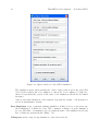
Stationary Simulation / RESTART is a variant of the steady-state simulation algorithm, which is especially useful for evaluating models with rare events (probabilities
smaller than 10−6 ) and is based on the RESTART method [17]. Estimation of those
events is a well-known problem in simulation algorithms, and usually requires extremely long simulation runs. To use this method, exactly one measure representing a
rare event must be defined. This measure must be of the form P{#Pi >= n}; or P{#Pi
<= n}; to measure the (small) probability that there are at least n (or not less than
n, respectively) tokens in place Pi in steady-state.
Figure 3.11 shows the option window for this evaluation algorithm. Most of the options
are equivalent to the ones already explained for the standard simulation above. The
max number of RESTART thresholds is an important parameter for the RESTART
technique and can be computed by the expected order of magnitude of the rare event
probability. A rule of thumb is to use the positive exponent of the expected small
probability, i.e. choose thresholds = 8 if the measured probability is about 10−8 . Some
parameters for the method are searched in a pilot simulation run, whose length can be
adapted in the according field.
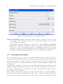
Transient Analysis computes and displays the transient solution of DSPNs, the behavior
of the net from the initial marking at time zero up to a specified point in time. No
general transitions are allowed for this evaluation.
TimeNET 4.0 User Manual — Net Class EDSPN
29
Figure 3.11: Option window for steady-state RESTART simulation
For the transient analysis of a DSPN at least one performance measure must be specified. Figure 3.12 shows the available options. The first and most important parameter
is the time until the transient evaluation should be carried out, measured in model
time units. The desired numerical Precision is given next. The output form tells the
program whether a graphical output of the transient behavior is wanted (curve) or not
(point). The values of the performance measures are computed and copied into the
model results for the final point in time in both cases.
The stepsize for output controls the points for which intermediate results are computed
and displayed. The result can be obtained in two ways, either by repeating Jensen’s
method or by storing and computing the matrix exponentials. The cluster size determines the number of steps for which one randomization is performed [5] in the case of
repeated randomizations. The internal stepsize can be adjusted to control the internal
discretization points.
30
TimeNET 4.0 User Manual — Net Class EDSPN
Figure 3.12: Option window for transient analysis
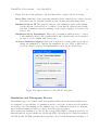
Transient Simulation estimates the initial behavior until a given time. It can be used
for any type of model, but is restricted to basic measures. Figure 3.13 shows the
corresponding option window.
The simulation is always running in sequential mode. The Number of sampling
points can be specified to adapt the resolution of the generated curves. If the Percentage rule is on, only a decreasing percentage of all sampling points need to reach the
predefined accuracy, otherwise this must hold for all sampling points. The remaining
settings have equivalent meanings like the ones for the steady-state simulation.
3.5
Evaluation Results
After a successful evaluation of the model, measure definitions in the model (see page 19)
are updated automatically and their result attribute gets the evaluation result. The result is
shown in the drawing area on the right side of the measure name. An already existing result
value for a measure is overwritten with the new result if a new performance evaluation has
been finished.
A performance evaluation also creates some text files with intermediate results (e.g. the
extended conflict set) and detailed output of the end results. These files are available in a
new directory which is named <modelname>.dir and is located in the same directory where
the current model is loaded from.
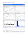
Some of these text files can be used to plot the result data with a tool such as gnuplot.
The following list describes the different text files based on their file extension. Note that
each type of performance evaluation creates only a subset of the following files. The main
TimeNET 4.0 User Manual — Net Class EDSPN
31
Figure 3.13: Option window for transient simulation
results can be obtained from the files <modelname>.RESULTS, <modelname>.STAT OUT,
and <modelname>.curves.
AUX Contains some auxiliary information of the performed evaluation. It contains the
solution method, model name, type of analysis, and some important evaluation settings.
curves Contains visualization data of all defined measures in the case of an experiment (a
set of analysis). This file can be used to plot the results with external tools.
DEFINFO Contains information about structural properties of the model, such as marking
dependent arc multiplicities, enabling functions of transitions, and marking dependent
transition weights.
ECS Describes extended conflict sets of the model.
ese Contains an estimation of the state space.
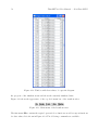
EXPRESULTS Contains a tabular list of results of an experiment. This file contains the
end result of each measure in each experiment step. It is possible to plot this file.
INV Contains the place invariants of the model.
pid Contains the list of software processes which are used to evaluate the model.
32
TimeNET 4.0 User Manual — Net Class EDSPN
pmf Contains the delay functions of all general transitions.
RESULTS Lists detailed results of given performance measures. This file contains the end
result of each measure as it is shown in the measure definition after a successful performance evaluation. Additional contents are the throughput values of timed transitions.
rrg Contains the reduced reachability graph (RRG) of the model in binary form.
siphons Contains the siphons of the model.
STAT OUT Contains results of the statistical analysis after a stationary simulation or
detailed results of a transient simulation.
STRUCT Contains structural information for internal usage.
tmark Contains the numbering of tangible markings of the model.
TN Contains the model in the .TN format, which has been used since TimeNET 2.0 and is
still taken as input by some evaluation methods. The graphical user interface generates
this file for an eDSPN model and starts the analysis afterward. The user interface is
also able to import models in this format. A description is available in Section B.
traps Contains the traps of the model.
Chapter 4
Stochastic Colored Petri Nets
In this section, the usage of TimeNET in the domain of stochastic colored Petri nets is
described. This class is called SCPN in TimeNET and is new in TimeNET 4.0. SCPNs
are especially useful to describe complex stochastic discrete event systems and are thus
appropriate, e.g., for logistic problems. The main difference between simple Petri nets and
colored models is that tokens may have arbitrarily defined attributes. It is thus possible to
identify different tokens in contrast to the identical tokens of simple Petri nets.
The introduction of individual tokens leads to some questions with respect to the Petri net
syntax and semantics. Attributes of tokens need to be structured and specified, resulting in
colors (or types). Numbers as arc information are no longer sufficient as in simple Petri nets.
Transition firings may depend on token attribute values and change them at firing time. A
transition might have different modes of enabling and firing depending on its input tokens.
The SCPN class in TimeNET uses arc variables to describe these alternatives.
The model objects (places, transitions, arcs, and textual elements) available in the net class
SCPN are explained in detail in Section 4.2. SCPN-specific features of the graphical user
interface and available simulation algorithms are covered in Sections 4.4 and 4.5. Advanced
features of TimeNET SCPNs include manual transitions, module concept, scriptiong engine,
and database integration. First-time readers should skip these later sections.
4.1
Colored Petri Nets
In the following we mostly point out differences to uncolored Petri nets. The syntax of textual
model inscriptions is chosen similar to programming languages like C++ or Java. The main
difference of stochastic colored Petri nets compared to standard Petri nets are the existence
of token types (colors) and the ability to hierarchically define the model. Both issues are
described shortly.
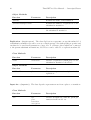
Token Types or Colors Tokens belong to a specific type or color, which specifies the
range of their attribute values as well as applicable operations just like a type of a variable
does in a programming language. Types are either base types or structured types, the latter
being user-defined. Available base types in the tool include Integer, Real, Boolean, String,
33
34
TimeNET 4.0 User Manual — Net Class SCPN
and DateTime as shown later in Table 4.3 on page 44. Structured types are user-defined and
may contain any number of base types or other structured types just like a Pascal record or
a C struct. Types and variables are textually specified in a declarational part of the model.
This is done with type objects in the graphical user interface of TimeNET, but is omitted
in the model figures. Variable definitions are not necessary in difference to standard colored
Petri nets because they are always implicitly clear from the context (place or arc variable).
Places Places are similar to those in simple Petri nets in that they are drawn as circles
and serve as containers of tokens. By doing so, they represent passive elements of the model
and their contents correspond to the local state of the model. As tokens have types in a
colored Petri net, it is useful to restrict the type of tokens that may exist in one place to one
type, which is then also the type (or color) of the place. This type is shown in italics near
the place in figures. The place marking is a multiset of tokens. The unique name of a place
is written close to it together with the type. The initial marking of a place is a collection of
individual tokens of the correct type. It describes the contents of the place at the beginning
of an evaluation. A useful extension that is valuable for many real-life applications is the
specification of a place capacity. This maximum number of tokens that may exist in the
place is shown in square brackets near the place in a figure, but omitted if the capacity is
unlimited (the default).
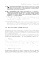
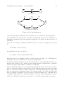
Hierarchical Models A SCPN model can be hierarchically defined. Each submodel is
represented by a substitution transition on the parent level. All input and output places of
the substitution transitions are connector places of the submodel and will be shown in each
submodel as dashed circles.
4.2
Objects and Attributes
This section lists and explains all available modeling objects in the SCPN net class.
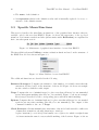
Figure 4.1: Model element buttons for net class SCPN
Figure 4.1 shows the model element button area for the net class SCPN in its initial state.
They are explained in the following together with their attributes.
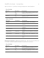
Places are depicted as circles.
• The text of a place is an identification string which is shown as a label nearby the place
in the model. When a place is created, it gets an initial name P plus a number. All
names of model elements must be unique.
• The queue of a place is the access strategy for the selection of tokens. Three different
types exists: ”Random” is the default strategy and returns tokens randomly. ”FIFO”
TimeNET 4.0 User Manual — Net Class SCPN
35
returns tokens in the order of arrival (just like in a queuing system). The opposite
strategy is ”LIFO”.
• The capacity of a place is the maximum capacity. It is the maximum number of tokens
the place can contain. A value of 0 represents an unlimited capacity and is the default
value.
• The tokentype of a place specifies the type of tokens for that place. As tokens have
types in a colored Petri net, it is useful to restrict the type of tokens that may exist in
one place to one type, which is then also the type or color of the place. This type may
either be a predefined base type or a model-defined structured type. The default type
is ’int’, the empty type is omitted.
• The watch attribute of a place denotes an automatic measure output. If this attribute
is ”true”, the number of tokens over time is measured and automatically displayed in
the result monitor (cf. Section 4.6) as a result measure.
Transitions are either timed or immediate transitions. The text of each transition is an
identification string (the name) and shown as a label. When a transition is created, it gets
an initial name ”T” plus a number.
Timed transitions are drawn as empty rectangles.
• Their firing delay is given as a timeFunction. Its default value is an exponentially
distributed firing time of 1.0. Currently, the following time functions are available:
Det(a) specifies a deterministic (constant) firing delay with the real value ’a’. Because
this is not really a function it is also allowed to write just a number into the field
timeFunction. Examples for a deterministic firing delay are Det(10.0) and 20.0.
Exp(a) specifies an exponentially distributed firing time with the mean (expected)
real value ’a’. The rate of this distribution is then ’1/a’.
Uni(a, b) specifies a continuous uniform distribution in the range between the real
values ’a’ and ’b’.
DUni(a, b) specifies a discrete uniform distribution in the range between the real
values ’a’ and ’b’.
Norm(m, v) specifies a normal distribution, also called Gaussian distribution. The
real parameter ’m’ is the mean value and parameter ’v’ is the variance (real value).
LogNorm(m, v) specifies a log-normal distribution. The real parameter ’m’ is the
mean value, and parameter ’v’ is the variance (real value), both of the underlying
normal distribution.
Wei(k, s) specifies the Weibull distribution with the real-valued shape parameter ’k’
and the real-valued scale parameter ’s’.
Triang(a, b) specifies a triangular distribution with lower limit ’a’ and upper limit
’b’. The triangle is isosceles.
36
TimeNET 4.0 User Manual — Net Class SCPN
A firing delay may depend on the current marking of the model. Each parameter of the
time function and the time function itself may thus contain references to definitions
and places. A definition is replaced by its current value and a reference to a place is
replaced by the number of tokens in this place. Page 40 provides a detailed description.
It is also possible to define an arbitrary, user-defined time function by overwriting
this function as described in Section 4.7. Please be aware that for consistency reasons,
transition firing times are specified as delays for all transition types. Firing rates of
exponential transitions have to be transformed into a delay by taking their reciprocal
value.
• Their globalGuard is a global firing condition. A global guard function restricts the
enabling of a transition. It is a boolean function that depends on the model state. A
transition with global guard ”#P 1 > 0 && #P 2 < 4” is only activated if there are
tokens in place P1 and less than 4 tokens in place P2. The #-sign means the number
of tokens in a place. A global guard function may contain references to definitions and
places. A definition is replaced by its current value and a reference to a place is replaced
by the number of tokens in this place. Page 40 has a detailed description.
• Their localGuard is a local firing condition. It is a boolean function that depends on
the input arc variables. The transition is only enabled with a certain binding of tokens
to variables in a model state if the guard function evaluates to ”true” for this setting.
A transition with an input arc variable ”Order” and a local guard ”Order.type == 3”
is only activated for tokens in the corresponding place, whose ”type” attribute is ”3”.
• Their takeFirst attribute can be used to speed-up the simulation in certain situations.
Typically, a transition creates bindings by considering all tokens of all input places and
selects one of these bindings randomly. If the takeFirst attribute is set to ”true”, only
one valid binding will be created and used. Note that the semantic of the Petri net is
changed. The takeFirst attribute is usable if there is no semantical assumption of the
token order.
• The serverType is either ”Infinite Server” or ”Single Server” (default value). It determines the way in which multiple customers are handled. Informally speaking, transitions with infinite server semantics can be enabled concurrently to themselves as
many times as there are enough input token sets available. This server characteristic is known from queuing theory. In case of a single server type the firing times are
determined sequentially.
• Their timeGuard is a global firing condition based on the simulation time. It is a function which returns the duration (a positive real value with double precision) until the
transition will be enabled. The transition is only activated if the value is 0.0. The current simulation time is provided by the ”NOW” value. A simulation time is internally
based on the DateTime class which has a lot of functions to create, manipulate, and
calculate time and date values. A detailed description of the DateTime functions can
be found in Section C.1. To enable a transition each Friday at 7:00:00 am, use the
following timeGuard: ”return (NOW.NextWeekDay(DateTime::fri, 7, 0, 0) - NOW);”.
TimeNET 4.0 User Manual — Net Class SCPN
37
• The specType is either ”Automatic” (default value) or ”Manual”. An automatic transition uses the given attributes to generate the appropriate simulation code as described
in Section 4.5. Sometimes it is necessary to overwrite the generated code manually
to allow special actions or complex behavior. Template classes are generated for each
manual transition if the simulation is started once. These templates can be used to
overwrite some of the generated code. The location and structure of these template
classes are described in Section 4.7.
• The manualCode attribute can be used to add manual code for overwriting the transition behavior as described in attribute specType.
• The watch attribute of a transition denotes an automatic measure output. If this
attribute is ”true”, the number of firings over time is measured and automatically
displayed in the result monitor (cf. Section 4.6) as a result measure.
• The logfileName is the name of an optional log file which will be written during a
simulation run if a logfileExpression exists.
• The logfileDescription specifies the first line of the log file. It can be used to have
textual headers for different logging columns. The headers can be separated by using a
double quote. A logfileDescription ”Delivered”Produced”Ordered” writes these three
strings separated by a TAB character to the log file.
• The logfileExpression contains expressions in C++-syntax which are evaluated on each
firing of the transition. The following expression variables can be used:
TAB produces the TAB character.
NOW writes the current simulation time.
<arcvariable> By using the name of an arc variable of one of the input arcs, the
corresponding token of the current binding can be accessed. Note that the data
type is equivalent to the type of the token.
<arcvariable.attribute> Like in programming languages, attributes of a complex
tokentype can be accessed by using a dot followed by the attribute name. If the
attribute is a complex tokentype itself, another dot can be used to access their
attributes and so on.
Assume a transition with two input arcs, one named with ”A” (structured type, attributes: ”name: string” and ”time: DateTime”) and the other with ”B” (type integer,
no attributes), then a valid logfileExpression is ”NOW, TAB, A.name, TAB, B, TAB,
(NOW - A.time)/(3600*24)”.
• The displayExpression contains one expression in C++-syntax which is evaluated on
each firing of the transition and is displayed as a result measure in the result monitor
(cf. Section 4.6). The expression syntax the same as for logfileExpression.
Immediate transitions are drawn as thin bars. Most of the attributes are already described
for timed transitions before. Additional attributes are:
38
TimeNET 4.0 User Manual — Net Class SCPN
• The priority is a natural number, that defines a precedence among simultaneously
enabled immediate transitions. The default priority is 1, higher numbers mean higher
priority. Timed transitions have always a lower priority than immediate ones.
• The weight is a real value (default: 1.0), specifying the relative firing probability of the
transition with respect to other simultaneously enabled immediate transitions that are
in conflict (compare [4] for the issue of how these values should be set correctly in the
context of GSPNs).
Substitution transitions are drawn as rectangles with two thin bars on each side. All of
their attributes are already described for timed transitions before. A substitution transition
contains one or more submodels which are connected to the parent model by the input and
output places of this substitution transition. One submodel (named replication) is created
by default and can be accessed by double-clicking the substitution transition. Section 4.4
describes how to add more replications and how to access different replications.
Module definitions are drawn as rectangles with the name ”Mod” inside. A module definition is an interface from a model instance to its environment, just like a substitution
transition. Additionally, it defines the parameters which can be set during instantiation.
Each module may have different implementations. All implementations have the same interface and one of them can be chosen at the time of the instantiation. More information about
the module concept is given in Section 4.8. Like substitution transitions, module definitions
are connected by common places with the model. The text attribute specifies the name of
the module. Names of input and output places correspond to the names of module inputs
and outputs.
Module instances are drawn as black rectangles. A module instance is a current implementation of a module. The text attribute of a module instance is an identification string
which is shown as a label nearby the module instance in the model. Two other attributes
must be given in a popup dialog window: The module attribute which is the name of the
module that should be instantiated, and the implementation attribute which is the name
of one of its implementations. The module instance is drawn together with its module pins.
These are small black rectangles. A module pin corresponds to an input or output (also
called common places) of the instantiated module. Exactly one place has to be attached as
an input or output to each pin. A double click on a module instance opens an editor window
to change parameter values which have to be previously defined in the module as described
on page 47.
An Arc is depicted as an arrow. To create an arc, select the source object with the left
mouse button, and drag the mouse with the button still pressed over the destination object.
Forbidden arcs disappear after releasing the button (e.g. arcs between transitions are not
allowed). While dragging the mouse over a destination object, a valid destination is shown
when the destination object changes into the selected state (gets a different color). To add
an intermediate point to the arc, double click on the arc at the desired position for this
intermediate point. A point is added at this position which can be moved to change the arc
position and can also be removed.
In contrast to simple Petri nets, where a number is the only attribute of an arc, the modeler
must be able to specify what kind of tokens should be affected and what operations on the
TimeNET 4.0 User Manual — Net Class SCPN
39
token attributes are carried out when a transition fires. This is done with arc inscriptions
which are defined by the attribute text. Arc inscriptions are enclosed in angle brackets <>
in figures.
Input arcs of transitions and their inscriptions describe how many tokens are removed during
transition firing, and attach a name to these tokens under which they may be referenced in
output arc and guard expressions. They carry a variable name in pointed brackets for the
latter task, optionally extended by a leading integer specifying the number of tokens to be
removed from the place. The default value for omitted multiplicities is one. A token from the
input place is given to the variable as its current value, and removed from the place during
firing. If a multiplicity greater than one is specified, the corresponding number of tokens are
bound to the variable and removed during firing. Each input variable identifier may be used
in only one input arc of a transition to avoid ambiguities.
A transition’s output arc defines what tokens are added to the connected place at the time
of the transition firing. There are two general possibilities for this: either existing tokens are
transferred, or new tokens are created. In the transfer/copy case the name of the chosen
input token is used at the output arc. The token that was bound to this input variable is
moved to the corresponding output place. The multiplicity of tokens must be the same to
avoid ambiguities, i.e. if three tokens are taken away from a place, there is no possibility of
transferring only two of them and arbitrarily removing one. For the same reason it is not
possible to use the same input variable at several output places. Arbitrary numbers of input
token copies can be made by creating new tokens and setting their attributes accordingly.
Table 4.1 contains examples for arc inscriptions including the syntactical expressions.
Input arc
Output arc
Meaning
<a>
<a>
Move a token a
< 2′ a >
< 2′ a >
Move two identical tokens a
< 2′ a >
< 3′ a >
Not allowed because of different multiplicities
<a>
< a(x = 5) >
Move token a and change attribute x to 5
<a>
< copy a >
Create a copy of token a
<a>
< new ({x = a.y}) >
Create a new token and set attribute x to
value of attribute y of a
<>
< new ({}) >
Create a new token with default attribute
values
Table 4.1: Examples for arc inscriptions of stochastic colored Petri nets
New tokens of the output place type are created if no input variable is specified at an output
arc. The attributes of a new token are set to their default values initially (c.f. Table 4.3 on
page 44). Attributes of new tokens can be set to specific values. The individual attributes of
the token (or the value if it is a base type) may be set to a constant value of the type or to
a value that depends on other input tokens. The elements of a structured type are again set
in angle brackets. Multiple new tokens can be constructed with a leading number and the
40
TimeNET 4.0 User Manual — Net Class SCPN
’ symbol. Operators are allowed in expressions as long as their resulting type corresponds
to the required one. In the special case where an element of a structured token should be
copied to create a new token, it is not necessary to write down all member attributes in
assignments. The member attribute in brackets is sufficient.
The type of the variables contained in the input and output arc inscriptions is implicitly
given by the type of the connected place and is thus not defined by the modeler. Restrictions
on the input tokens are modeled using transition guards as already described.
Performance measures are depicted in the model by a string ”name = expression”. They
can be created by using the button named ”R=” in the object button area. A performance
measure defines what is computed during a simulation. A typical value would be the mean
number of tokens in a place. Depending on the model, this measure may correspond to the
mean queue length of customers waiting for a service or to the expected level of work pieces
in a buffer. Measures have the following attributes:
• Attribute eval defines the type of this measure. Three different types are available:
Instantaneous measures display the instantaneous value of the given expression over
time.
Cumulative measures display the cumulative value of the given expression over time.
TimeAverage measures display the average value of the given expression over time,
i.e. the cumulative value divided by the model time.
• If watch is true, then the measure will be automatically displayed as a result measure.
• The result is the name of the measure.
• An expression which should be evaluated.
A performance measure expression can contain numbers, definitions, algebraic operators,
and place references (written as #<placename>). Examples of performance measures are
#P5+#P8; and N/(5*#P2)+#P1; while N is a valid definition.
A constant definition which can be used in other expressions is depicted as a string ”name
:= expression”. They can be created by using the button named ”D=” in the object button
area. After defining N := 5 it is possible to write N in any place or transition where a number
is allowed. But it is important to keep the type of the definition correctly, because 4 is an
integer value while 4.0 is a real value. Definitions have the following attributes:
• The result is the name of the definition.
• An expression which is the definition value and is internally replaced for every occurrence of the definition name.
It is possible to place a comment into a SCPN model to increase understandability. The
corresponding button shows an exclamation mark (’ !’). A comment is a user-defined string
TimeNET 4.0 User Manual — Net Class SCPN
41
which is given in the attribute commentText. Comment objects will be ignored during simulation and have no effect for the evaluation of result measures.
A recordTokentype defines a structured data type as described later on page 44. It is shown
in a white oval in the model. The button has the same sign. A recordTokentype extends the
included set of basic types to increase the modeling possibilities. A recordTokentype must
have a unique name and may contain an unlimited number of attributes. Figure 4.2 shows
the dialog window to set the attributes. The tokentype of a place has to be a basic type or
one of the defined tokentypes.
Figure 4.2: Window to define a new tokentype in a SCPN model
External token type and module definitions can be imported by using the libImport feature.
The corresponding button contains a white rectangle with the name ”imp” in it. A file dialog
is opened to choose an external SCPN model which contains token type or module definitions.
After choosing an appropriate file, a white rectangle is placed in the model which shows the
filename. A libImport has a filename attribute which contains the full path to the external
model. The definitions of the imported model can be used in the current model. Modules
can be instantiated and token types can be used. All definitions which are used from the
imported model will be temporarily copied into the current model just before a simulation
starts.
4.3
SCPN Expressions
A lot of attributes of components are represented by expressions which will be described in
the following.
4.3.1
Constants
The most commonly used class of expressions are constants. A constant expression is statically evaluable and represents an initial parameter. The simulation state is not accessible.
42
TimeNET 4.0 User Manual — Net Class SCPN
However, a constant may consist of a complex arithmetical or boolean expression, and may
reference a value parameter as described on page 45.
Place capacities and transition firing delays are examples for constant expressions. The data
type of a constant expression derives from the corresponding context: place capacities are
always integer values, firing delays are always real values.
4.3.2
Functions
Some object attributes allow expressions which are represented by functions. A function
mostly depends on the simulation state. Local and global guards are an example for functions
which evaluate to a boolean value. How a function is accessing the state of the simulation is
varying and specified in the description of each modeling object.
Three basic types of references to state values exists:
• References to places.
• References to definitions and measures.
• References to tokens and their attributes.
4.3.3
Place References
Some functions allow references to places. Such a reference is replaced by the current number
of tokens in this place during runtime of the simulation. Place references are depicted by a
hash mark (’#’) followed by the name of a place. Two variants for decomposing the name
of a place exists.
If the name of a place is a simple name (e.g. #P1), the corresponding place object will be
initially sought in the current submodel. If it could not be found, the search continues in
the parent submodel until the root model (or in case of a module definition, the module
implementation) is reached.
Complex place names contain a path of substitution transitions with a replication identifier
other than that mentioned place name. For instance, #subTrans1[0].subTrans1 1[2].P2
refers to place P2 which is in the second replication of submodel subTrans1 1 which in turn is
in the submodel subTrans1. Each submodel is referenced by the name of the corresponding
substitution transition. Places inside a module implementation cannot be referenced from
outside but may be accessed by definitions.
4.3.4
Definition and Measure References
All functions which allow place references also allow references to definitions and measures.
A reference to these kind of expressions is depicted just by the name. It is for instance
possible to reference a definition with name ”D1” in an exponentially distributed transition
firing delay by typing Exp(D1).
TimeNET 4.0 User Manual — Net Class SCPN
43
In contrast to place references it is possible to reference definitions which are part of a
module instance by using the instance name. In this case, the definition has to be defined in
each module implementation of the corresponding module. Other definitions are not visible.
The expression subTrans1[0].modInst1.D3 references definition D3 of the module instance
modInst1 in the first replication of the substitution transition subTrans1.
4.3.5
Token and Attribute References
Some attributes of transitions (e.g. local guards) and output arcs facilitate access to incoming
tokens and their attributes. Each token is uniquely identified by the inscription of the input
arc which is used to reference these tokens. An attribute of a token can be accessed by the
token name followed by a dot (’.’) and the attribute name. Is the attribute a member of a
structured data type, their child attributes can be accessed similarly. Examples:
tokenX References token tokenX.
tokenX.color References attribute color of token tokenX.
tokenX.color.red References attribute red of attribute color of token tokenX.
4.3.6
Operators
Table 4.2 outlines the operators which are available in arithmetic and logical expressions.
Priority
Operator
8
7
(. . .)
+, −
!
∗, /, %
+, −
<, <=
>, >=
==, ! =
&&
||
6
5
4
3
2
1
Type
arithmetic
logical
arithmetic
arithmetic
arithmetic
arithmetic
primitive
logical
logical
Executed operation
brackets
unary plus, unary minus
NOT
multiplication, division
addition, substraction
lower than, or lower or equal
higher than, or higher or equal
equal, unequal
AND
OR
Table 4.2: Possible operators in stochastic colored Petri nets
4.3.7
Basic Data Types
TimeNET supports five basic data types. Table 4.3 shows each type with some examples.
44
TimeNET 4.0 User Manual — Net Class SCPN
Type
Name
Default value
Examples
Integer
int
0
732
Real
real
0,0
9,56
Boolean
bool
false
true, false
String
string
””
”foo”
Date/Time
DateTime
0:0:0@1/1/0
NOW, 11:23:46@03/27/2007
Table 4.3: Base types in stochastic colored Petri nets
Integer values are internally stored as int values. The range of values is between −231 =
−2147482648 and 231 = 2147483647 on a 32 bit system. Integer values can by checked
for equality and inequality (==, ! =), can be compared (>, <, >=, <=), and arithmetically combined (+, −, ∗, /, %).
Real values are internally stored as double values with a codomain of about ±1.7 ∗ 10308
with a precision of 15 digits. The same operators are defined as for integer values.
Boolean values are internally stored as bool values which represent false or true. Possible
operators are the checks for equality and inequality (==, ! =), and the logical operators
conjunction (&&), disjunction (||), and negation (!).
String values are constant strings bordered by double quotes. The typical C escaping mechanism is applicable: Quotation marks and the backslash sign are prefixed by a backslash
(\). A tabulator can be written as \t and a new line as \n.
Date/Time values are internally stored as objects of the DateTime class. Appendix C.1
describes all methods of this class. The DateTime class internally uses a double value
which makes the Date/Time values uncountable. But it provides for practical reasons
the hh:mm:ss@MM/dd/yyyy format which is often used for input and output. The
global variable NOW always represents the current simulation time. DateTime values
can by checked for equality and inequality (==, ! =), and can be compared.
4.3.8
Structured Types
Basic data types are not sufficient for SCPN models. TimeNET supports a datatype system
that is comparable with structs in the programming language C. A structured type can be
defined in the model. It consists of several attributes, each has to be either a basic type
or an already defined structured type. The graphical editor window which is used to create
a structured type has been shown on page 41. The literal NULL may be used to check a
structured type for emptiness.
TimeNET 4.0 User Manual — Net Class SCPN
4.3.9
45
Value Parameters
A value parameterization allows the usage of placeholders for attribute values which are
replaced by a current value before the simulation starts. Test series with varying parameters
are possible. Value parameters are only available for basic types and can be declared at
the root level of a SCPN model or in a module definition. A value parameter in a module
definition has a predefined value which can be overwritten in each module instance. The
parameter value either has a literal value of the corresponding type or is the name of a
parameter of a parent model level. Each value is hierarchically top down inherited. A dollar
sign (’$’) extended by the name of a parameter is used to reference a value parameter. The
expression $numPar can be used as a place capacity if numPar is a value parameter of type
int.
4.4
Specific Menu Functions
This section describes the miscellaneous functions of the graphical user interface that are
available only for the net class SCPN. Figure 4.3 shows the appearance of the top level menu
bar.
Figure 4.3: Main menu of graphical user interface for net class SCPN
The first additional menu SCPN contains items to create and select replications and to
navigate through submodels. Additionally, it contains SCPN net class specific functions
such as a syntax check, a Javascript controlled simulation, a template generator for manual
transitions, and a parameter control for SCPN modules. This additional menu is shown in
Figure 4.4.
Figure 4.4: Menu SCPN for net class SCPN
The additional functions are described in the following.
46
TimeNET 4.0 User Manual — Net Class SCPN
Descend The last shown replication/implementation of the underlying submodel is displayed in the editor window. It is the same action as doubleclicking a substitution
transition or module definition. Menu item Ascend is the reverse operation and displays the parent model of a submodel. This item is available if a substitution transition
or a module definition is selected.
Ascend The parent model of the submodel will be displayed. It is the reverse operation to
menu item Descend. This item is available if a submodel of a substitution transition or
an implementation of a module definition is currently displayed in the editor window.
Next Replication The next replication/implementation is then displayed in the editor
window. This item is available if a submodel of a substitution transition or an implementation of a module definition is currently displayed and several replications or
implementations exists.
New Replication A new replication/implementation is created and displayed in the editor window. This item is available if a submodel of a substitution transition or an
implementation of a module definition is currently displayed.
Remove Replication The currently shown replication/implementation is removed and the
previous one is shown in the editor window. The first replication/implementation (replication 0) cannot be removed. This item is available if a submodel of a substitution
transition or an implementation of a module definition is currently displayed.
Run Script Opens a window to setup a Javascript environment and allows to run such
a script which, e.g., controls a simulation. Detailed information about the TimeNET
scripting engine can be found in Section 4.9.
Figure 4.5 shows the setup window for the scripting engine. This window has the
following entries:
Script file Full path of the script file which should be started. Normally, scripts are
stored in the directory TimeNET/SCPNScripts.
Source net file Full path of the SCPN model which should be used. The default entry
is the currently opened SCPN model. The given model file is passed through the
Javascript engine and is available as arguments[0] in the script.
Destination net file Full path of a temporary SCPN model which can be used in
the script file to store the model modifications. The given destination filename
is passed through the Javascript engine and is available as arguments[1] in the
script.
Integration property file This file is required to setup the OpenAdaptor framework which can be used by Javascript to access different database connections.
A default integration property file (which is automatically set) can be found in
TimeNET/etc/gpsc conf/integration.props. Normally, this file does not need
to be changed.
Log4j property file This file is required to setup the Log4J framework which is internally used by OpenAdaptor. A default Log4J property file can be found in
TimeNET 4.0 User Manual — Net Class SCPN
47
Figure 4.5: Window to start a Javascript script for controlling a SCPN simulation
TimeNET/etc/gpsc conf/log4j.props and is automatically set. Normally, this
file does not need to be changed.
Open destination net file If this option is enabled, the destination net file is opened
after running the script.
Skip integration If this option is enabled, the database integration is not performed.
Activate this option if the script does not need database access.
Generate Template Creates template files (.c and .h) for a manual transition which
must be selected before. These template files can be used to overwrite the transition behavior such as guard functions. A detailed description of manual transition
is given in Section 4.7. Both template files are created in a special directory named
<modelname>.manual within the current model directory.
Edit Parameters Opens a window to add and edit value parameters of a SCPN model as
shown in Figure 4.6. A parameter consists of the following values:
Type The data type of the parameter value. This must be a basic type.
Name The name of the parameter. A parameter is referenced in expressions by using
this name.
48
TimeNET 4.0 User Manual — Net Class SCPN
Default value The default value which is normally used. If the parameter is assigned
to a module, this value can be overwritten in each module instance.
Description Optionally a parameter may store a short description which is otherwise
not used.
Figure 4.6: Window to add/edit parameter values for SCPN models
Check net Validates the model in the currently selected editor window. This is done by
validating the underlying XML model against the given SCPN XML-schema. All XML
schema definition files are located in TimeNET/etc/schemas. A lot of structural and
syntactical properties are specified in the XML-schema. Most of the structural properties are automatically considered by the TimeNET GUI. Expressions and some more
structural properties are also checked by using an internal ANTLR grammar scheme for
SCPN which additionally validates the syntax of expressions. Note that not all expressions can be validated. Some of them might give errors when starting the simulation.
An example of a syntax error is shown in Figure 4.7.
Figure 4.7: Example of a syntax error after Check net
TimeNET 4.0 User Manual — Net Class SCPN
4.5
49
Simulation
This section explains the performance evaluation of TimeNET for the SCPN net class. The
complexity of this net class only allows a simulation to get performance measures. Simulation
is accessible via the Simulation menu, which is shown in Figure 4.8.
Figure 4.8: Menu structure of SCPN simulation
The following items are available in the Simulation menu.
Start Simulation simulates the selected SCPN model.
Figure 4.9 shows the applicable options which will be described in the following.
Start Time Start time of the simulation in the format hh:mm:ss@mm/dd/yyyy. This
time is used to initialize transitions and calculate their first firing times.
End Time End time of the simulation in the format hh:mm:ss@mm/dd/yyyy. If the
simulation has reached this time by firing a transition, the simulation is stopped.
Simulation Server IP This is the IP address of the simulation kernel. If the simulation should run locally, the IP is ”localhost”. If another IP address is used, make
sure that a simulation kernel is running on the target computer, as described in
Section 4.10.
Simulation Server Portnumber This is the port number which is used to connect
to the simulation kernel. The default value is 4445 but this value can be changed
in order to avoid conflicts with other ports.
Result Server IP This is the IP address of the result monitor. If the Result monitor
should run locally, the IP is ”localhost”. If another IP address is used, make
sure that a Result monitor is running on the target computer, as described in
Section 4.6.
Result Server Portnumber This is the port number which is used to connect to
the result monitor. The default value is 4444 but this value can be changed in
order to avoid conflicts with other ports.
Random seed value Can be used to specify a seed value for the random generator.
The default value is 0, then the current milliseconds of the system clock is used.
A value different from 0 is useful to get the same order of executions for multiple
simulation runs.
Activate simulation logging If this item is activated, several logfiles are produced
during the simulation to analyze the simulation process. These logfiles will be
stored in a newly created folder <modelname>.log in the model directory.
50
TimeNET 4.0 User Manual — Net Class SCPN
Figure 4.9: Option window for the SCPN simulation
The simulation starts when pressing the ”Start” button and stops at the given End
Time. If the result monitor is configured to run at the local computer (”localhost”),
then it is automatically opened at the start of the simulation and shows all defined
measures.
After a successful simulation a file results.log with the results of all measures is
stored in <modelname>.result.
Stop Simulation stops a currently running simulation. If this does not work, please use
the TaskManager on Windows or the ”kill” command on Linux to stop the simulation
process. The name of a simulation process equals the name of the simulated model and
has on Windows systems the file ending ”.exe”.
Tokengame starts a step by step simulation of the selected model.
TimeNET 4.0 User Manual — Net Class SCPN
51
Figure 4.10 shows the applicable options which will be described in the following.
Start Time Start time of the tokengame simulation in the format hh:mm:ss@mm/dd/yyyy.
This time is used to initialize transitions and calculate their first firing times.
Simulation Server IP This is the IP address of the simulation kernel. If the simulation should run locally, the IP is ”localhost”. If another IP address is used, make
sure that a simulation kernel is running on the target computer, as described in
Section 4.10.
Simulation Server Portnumber This is the port number which is used to connect
to the simulation kernel. The default value is 4445 but this value can be changed
in order to avoid conflicts with other ports.
Activate simulation logging If this item is activated, several logfiles are produced
during the simulation to analyze the simulation process. These logfiles will be
stored in a newly created folder <modelname>.log in the model directory.
Figure 4.10: Option window for the SCPN token game
Simulation and Tokengame Process
The simulation process consists of various steps which will be shortly described in this section.
A tokengame is a special kind of a simulation and is covered also in this section. It includes
an activity control mechanism for the simulation process. Differences between a tokengame
and a standard simulation will be pointed out at the respected places.
After starting the simulation of a model, the corresponding XML document is parsed by an
internal abstraction layer which is also used in the GUI to check the model. This layer includes
a SCPN specific ANTLR grammar that represents a more detailed structural description of
52
TimeNET 4.0 User Manual — Net Class SCPN
the SCPN class than the XML schema. A lot of structural and syntactical properties can
be verified by using this grammar. Model objects and its relationships are stored in internal
classes which are built automatically from the ANTLR grammar.
The abstraction layer is able to generate C++ code for all tokens, transitions, and measure
objects from a SCPN model. These files will be stored in a special folder (containing 32
random digits) inside the model directory. The code for manual transitions is copied to this
directory as well. A buildnet class is generated to reconstruct the model structure from the
generated objects. This is the starting point of the simulation.
A makefile is copied to the same directory and executed afterward. It compiles the generated files and links all compiled objects with a simulation kernel which is already built in
TimeNET. The output is an executable simulation program which is started by the GUI.
The name of this program is <modelname>.exe.m which is started by the GUI. The name
of this program is <modelname>.exe.
The initial marking is saved by the abstraction layer into a file marking.xml which is loaded
from the generated simulation program. This is started with some arguments which are
provided by the GUI from the input of the simulation dialog. These arguments capture
knowledge about the IP address of the result monitor and the simulation time.
If the simulation runs in tokengame mode, it stops after each simulation step and transfers
the current marking to the GUI. After the user has chosen a transition to fire, its name is
transferred back to the simulation which does the next step.
4.6
Result Monitor
The result monitor is a TimeNET component which is used to graphically display result
measures of a SCPN simulation. Figure 4.11 shows the main window of the result monitor
after running a simulation. It is divided into a number of subwindows, each of them showing
a diagram of result measures. The title of a subwindow contains the name and type of the
corresponding measure. All windows can be resized and arbitrarily placed inside the main
window.
Two different types of charts are available: A bar chart which is shown in the right bottom
window and a line chart which is used in all other windows in Figure 4.11. Line charts
typically show the period of time on the horizontal axis. Discrete values on the vertical
axis represent value changes of a measure at a specific point in time. By default, points are
connected by a line. Bar charts show rectangular bars of lengths usually proportional to the
magnitudes or frequencies of what they represent. Bar charts are used for comparing two or
more values. The bars are always vertically oriented.
A legend can also be displayed in each diagram. Line charts may also show the mean line and
the gliding mean line of the corresponding values. It is also possible to display the original
data values in a separate window as shown in Figure 4.12.
It is possible to zoom into a line chart by defining a visible area. The start point of this
area is chosen by clicking with the left mouse button into the drawing area of a diagram
and drag the mouse to another location. After releasing the mouse button, the diagram only
TimeNET 4.0 User Manual — Net Class SCPN
53
Figure 4.11: Result monitor window which displays results from a simulation
shows the defined area. A reset to the original zoom is possible by doubleclicking with the
left mouse button into the drawing area.
Typically, the result monitor is automatically started when running a simulation and shows
the results immediately. In the upper part of the main window is a status bar named VectorCache which displays the level of the internal cache. There is a second gauge that visualizes
54
TimeNET 4.0 User Manual — Net Class SCPN
Figure 4.12: Window with data values of a specific diagram
the progress of the simulation run and shows the currently simulated time.
Figure 4.13 shows the appearance of the top level menu bar of the result monitor.
Figure 4.13: Main menu of the Result monitor
The first menu File contains the typical open and close functions as well as export functions
for data values. It is shown in Figure 4.14. The following commands are available:
TimeNET 4.0 User Manual — Net Class SCPN
55
Figure 4.14: Menu File of the Result monitor
Open Allows to open a set of data values. This function is currently not available.
Close Closes the currently selected subwindow.
Close all Closes all subwindows.
Export values Allows to export the original values of the currently selected subwindow.
This function opens a file dialog to choose the target location for the created file. The
file is stored in the csv format, so it contains a list of semicolon (not comma) separated
values which can be loaded into Microsoft Excel and other programs.
Export SVG Image Allows to export the image of the currently selected subwindow in
the SVG (scalable vector graphics) format. A SVG image is supported by some open
source programs and also by a lot of commercial programs such as Adobe Illustrator.
Exit Exits the result monitor.
Some display options are available in the second menu Display which is shown in Figure 4.15.
The following commands are available:
Figure 4.15: Menu Display of the Result monitor
56
TimeNET 4.0 User Manual — Net Class SCPN
Property Opens a dialog window to change the properties of one or all subwindows. This
window is shown in Figure 4.16. All available options are described separately in this
paragraph because they are also available as individual menu items. The property
dialog allows to set specific properties for all chart windows in one step.
Figure 4.16: Dialog window to edit the display properties
Chart type This menu item sets the type of the chart of the currently selected window. It
is possible to select a line chart or a bar chart.
Line If activated, a line is drawn in the diagram between all data values. This option is only
available for line charts and is set by default.
Points If activated, a point is drawn for each data value. This option is only available for
line charts.
Mean Line If activated, a line which represents the arithmetic mean is drawn for all data
values. This line is drawn green colored. This option is only available for line charts.
Gliding mean line A/B If activated, a line which represents the gliding mean is drawn
for all data values starting with a specific time and date. A dialog window is opened
to enter the start time. This option is only available for line charts.
Rectangle line If activated, a rectangle line is drawn in the diagram between all data
values. The line is drawn blue colored. This option is only available for line charts.
Legend If activated, a legend is shown in the currently selected diagram. Some diagrams
in Figure 4.11 have the legend activated.
TimeNET 4.0 User Manual — Net Class SCPN
57
Show full chart If activated, the full chart is shown after receiving start and end time.
Otherwise the horizontal axis grows after receiving new values.
Data values Opens a separate window which shows the original data values in a table.
Such a table is depicted in Figure 4.12.
Parameters of the horizontal x-axis and the vertical y-axis of a selected diagram can be
changed by using the menus X-Axis and Y-Axis, exemplarily shown for the x-axis in
Figure 4.17. The following commands are available:
Figure 4.17: Menu X-Axis of the Result monitor
Grid If activated, a grid is shown in the selected diagram.
Axis format Should be used to define the data type which is used to interpret and show
the values on the axis. The following datatypes are possible: Number, Date, Time, and
Date/Time. The default setting for the x-axis of a line chart is Date/Time and for the
y-axis it is Number. Bar charts always show an integer number on the x-axis. Note
that the x-axis of a bar chart is on the left side.
Range Defines the value range of the axis. A new dialog is shown where the lower and
upper boundary of the range can be specified. In the default settings, the x-axis shows
the complete time range of the simulation run and the y-axis starts with the lowest
value and stops at the highest value.
Autoview Resets all properties of this axis to the default settings.
The alignment of all diagram windows can be chosen in the last menu Window which is
shown in Figure 4.18. The following commands are available:
Auto tile If activated, the currently selected diagram window is automatically relocated to
fit into the current tile structure.
Tile Relocates all diagram windows in the main window by using a tile structure. The
windows are displayed in tiles, one beside another.
List Relocates all diagram windows in the main window by using a list structure. The
windows are displayed at the full width, one after another.
Cascade Relocates all diagram windows in the main window by using a cascaded structure.
The windows are displayed staggered one behind another.
58
TimeNET 4.0 User Manual — Net Class SCPN
Figure 4.18: Menu Window of the Result monitor
Window list A list of all opened windows is displayed. By selecting one window from this
list, the corresponding diagram window will be activated and moved to the front. The
currently active window is shown by a checkmark.
4.7
Manual Transitions
A manual transition allows individual C++ implementation of transition behavior and requires a very good knowledge of internal simulation processes. It is defined by setting the
specType attribute of any transition to ”Manual” as described on page 36. This section covers
a short survey of the implementation. It is not possible to give a full specification for manual
transition code because it depends on some internal structures which are not available for
public. As described later in Section 4.5, each modeled transition is translated into C++ code
which can be found in a special folder in the model directory. This generated implementation
is a very useful hint for the own C++ implementation of manual transitions.
Two methods exist to generate template classes for a manual transition which can be used
for individual C++ implementation: (1) The ”Generate Template” item in the SCPN menu
(see Section 4.4) creates the template class for a selected manual transition. (2) Template
classes for all manual transitions are created after starting a (temporary) simulation.
For each manual transition, a C++ source file (.c) and a C++ header file (.h) will be created
in a special directory named <modelname>.manual in the currently used model directory.
This is only done if there is no class with the same name. The location of a template class
is the same location which is used by the simulation to load the manual transition code.
A template file contains some special code which is depicted by square brackets. The following
list describes these items which are also explained as a comment in each template file:
<ignore> Text which indicates that all characters that follow in the same line should be
ignored and will be removed during code generation.
TimeNET 4.0 User Manual — Net Class SCPN
59
<comment> Text which indicates the beginning of a block of one or more lines which will
be ignored and removed during code generation. The comment region ends at the token
</comment>.
<classname> Text for the class name.
<parent> Text for the parent class name.
<headername> Text for the name of the header file’s define.
It is recommended to keep those text parts and add/edit only constructor and method code.
Also, it is recommended to modify only methods whose behavior cannot be clearly defined
by the GUI. All other methods should be removed from the template. If a method does
not exist, the parent method automatically uses the default behavior which considers the
corresponding transition attributes from the model.
The constructor of a manual transition automatically calls the parent constructor of the
internal transition class. It should not be changed but can be used to initialize new class
variables.
Methods which are important for specifying additional behavior are described in the following.
bool globalGuard() Returns true if the global guard function is satisfied. This method is
called after a change in an input or output place of the transition to check for enabling.
It normally uses net->getPlace(<placename>) to find a place in the model and
checks the current marking size by using the method place->getMarkingSize().
void initGlobalGuards() Registers this transition as a global guard listener of places
and is called once in the beginning of the simulation. Each place which is referenced
by the global guard function of this transition needs to be informed. The method
net->getPlace(<placename>)->addGlobalGuardTransition(this) is used to register each place.
void moveTokens(TokenList &binding) Moves tokens from places to other places. It
is executed if a transition fires. The default implementation moves tokens from all
input places to all output places according to the arc inscriptions. Parameter binding
contains the current binding which is a set of tokens to be moved. Tokens can be
removed from a place by calling place.removeToken(token) and added to a place by
calling place.addToken(token).
TempBindingList* generateBindingList() Generates a list of all possible bindings for
this transition. It is called to create bindings if all preconditions to enable the transition
are fulfilled. The default implementation uses a permutation of all tokens in all input
places with respect to the transition attributes such as takeFirst. Each binding is a set
of tokens which is represented by a TokenList.
bool hasTimeguard() const Returns true if this transition has a time guard and is called
to speed-up the check for the timeguard function.
60
TimeNET 4.0 User Manual — Net Class SCPN
Seconds T Timeguard(const DateTime &now) Returns the duration when the transition could be enabled based on the given time now. If this method returns 0.0 the time
guard is satisfied and the transition can be enabled immediately. A detailed description
of the DateTime class is given in Appendix C.1.
Seconds T getFiringDelay() const Returns a tangible firing delay. It is called when a
binding is created. This method uses the class Delay as described in Section C.2 which
contains some important delay functions such as exponential or normally distributed
random delay. It is possible to implement an own delay distribution which not necessarily needs to be a continuous function.
double display(TokenList &binding) Returns a value which is displayed as a result
measure in the result monitor after each firing of this transition. The default implementation uses the attribute displayExpression. This method has access to the currently
fired binding which can be evaluated to return a measure.
void log(TokenList &binding) Writes a number of values to the logging output after each
firing of this transition. The default implementation uses the attribute logExpression.
This method has access to the currently fired binding which can be evaluated to write
out the measure. The constant name translogfile has to be used as the output stream.
4.8
Parametrizable Module Concept
Modularization is a key concept of software and model design. It allows to outsource multiply
used functionality into a library. A module definition provides an interface to integrate an
instance of a module into the environment. This interface also defines the parameters which
can be set during the instantiation.
Other than adjusting value parameters, also the structure of the implementation should be
exchangeable. A module definition may hold several alternative implementations which have
the same interface. During the instantiation, one of these implementation can be chosen.
4.8.1
Modules
Modules are created by placing a module definition into the model as described on page 38.
Such like a substitution transition, inputs and outputs are represented by places which are
connected to the module definition by arcs as shown in Figure 4.19. The inscription of
a module definition forms the name under which it can be instantiated. The names and
tokentypes of all input and output places are equal to the names of the inputs and outputs
of the module and their types.
4.8.2
Module Implementation
The implementation of a module can be edited in a separate page of the model. This page is
accessible by doubleclicking the module definition or use the Descend action just like a substitution transition. A module implementation is equivalent to a submodel of a substitution
TimeNET 4.0 User Manual — Net Class SCPN
61
Figure 4.19: A module definition with two inputs and one output
transition and has an own label for identification. In an implementation view of a module,
inputs and outputs are drawn as dashed places.
Different implementations of a module can be created by using the New replication action
in the SCPN menu as described on page 45. Each replication represents an alternative implementation for this module. Actions to delete replications and switch between replications
have been already described on page 45.
4.8.3
Module Instantiation
In difference to substitution transitions, multiple instantiations of a module may exist. A
module instance can be created by using the moduleInstance button as described on page 38.
Input and output pins are created automatically which represent placeholder transitions for
the module inputs and outputs. They provide an assignment for the inputs and outputs and
can be connected to normal places.
The three important steps to create and use a module are depicted in Figure 4.20.
If the simulation (or a tokengame) is started, a module instance is internally converted
to a substitution transition which holds the selected implementation as its submodel. The
places which are attached to the module pins are then equal to the common places in the
module implementation. Figure 4.21 shows the substitution transition and the corresponding
submodel which have been created before the simulation starts.
4.9
TimeNET Scripting Engine
TimeNET 4.0 provides a scripting engine for the SCPN net class. This engine allows a scriptcontrolled generation and modification of SCPN models as well as an automated start of the
simulation with different parameters. The script needs to be written in Javascript, a well
known scripting language most often used for client-side web development.
An editor for the script development is not integrated into TimeNET. Each available editor
can be used. Example scripts are located in the SCPNScripts directory.
62
TimeNET 4.0 User Manual — Net Class SCPN
(a) Definition
(b) Implementation
(c) Instantiation
Figure 4.20: Module implementation and instantiation
The Javascript engine in TimeNET supports a data warehouse by supporting OpenAdaptor,
an EAI (Enterprise Application Integration) software. It provides many ready-built connectors that include JMS, JDBC, IBM MQ Series, TIBCO Rendezvous, TCP/IP Sockets,
SOAP, HTTP and Files. It provides exception management and scriptable components for
data filtering, transformation and validation.
A script does not belong to a specific model, but if the script modifies some parts of a model,
it must be ensured that these components exists in the model.
Starting a script is either possible by using the Run script item of the SCPN menu or by
using the batch files run (Linux) or run.bat (Windows) in the SCPNScripts directory. The
following parameters can be used in the batch file:
Parameter
-s
-m MODELDIR
-i INTEGRATION
Description
Disables the database integration (optional)
Path to the model directory to resolve relative paths
Specifies the integration.props file for data integration
Additionally, the configuration file for the Log4j subsystem is given as a system property
value -Dlog4j.configuration$LOG4J-CONF in each batch file. To use the TimeNET home
directory inside the scripts, it is specified by -DTNETHOME=$TNETHOME.
4.9.1
Creating Javascript scripts
In addition to standard Javascript language elements like data types, operators, and control
structures, a special SCPN modeling and simulation interface is provided. All required SCPN
TimeNET 4.0 User Manual — Net Class SCPN
63
(a) Substitution
(b) Substitution submodel
Figure 4.21: Module substitution
objects such as places, transitions, arcs, measures etc. are available as Javascript classes.
The TimeNET Javascript interface is explained in Appendix D and a Javadoc HTML documentation (jsapi-doc.zip and jsapi-doc.tgz) can be found in the docs directory of
TimeNET.
The basis for creating or modifying a SCPN model is a net object. An empty net is created
by:
var newNet = Net.create();
An existing model can be loaded by:
var oldNet = Net.load(filename.xml);
After this step it is for example possible to search for places by name or to add transitions.
All possible objects and functions are described in Appendix D.
To include external data into the model, the data needs to be successfully integrated into the
internal data warehouse. Two methods exist: directly integrate external data or integrate
formerly integrated data which are available in a XML file.
Data in the internal warehouse can be queried by using XPath queries. A reference documentation to XPath is available in Appendix D.2. Three different result types exist: (1) results
that are returned by string and can be analyzed by Javascript string functions, (2) results
that are returned as a string array where each element matches one result, and (3) results
that are returned by ResultNodes. The last type is the most flexible type. A ResultNode is
a simplified XML-DOM-Node which has functions to get the value, its attributes, and the
child nodes. With this result type it is possible to work with complex subtrees as results.
64
4.9.2
TimeNET 4.0 User Manual — Net Class SCPN
Integration of external data
OpenAdaptor (https://www.openadaptor.org) is used to connect external data to the scripting engine. A simple example should describe this process.
First, the Adaptor Framework Editor (AF Editor, part of OpenAdaptor) must be started.
This can be done by running bin/openadaptor framework editor.bat which opens the
program as shown in Figure 4.22.
Figure 4.22: Adaptor Framework Editor window
As an example we want to connect to a SQL database as a source for our data to reveal a
possibility to attach and configure external data repositories.
TimeNET 4.0 User Manual — Net Class SCPN
65
The AF Editor is responsible for adding data sources such as an JDBC capable SQL database
to the OpenAdaptor system and to configure their behavior. It creates a configuration file
which must be an argument for OpenAdaptor later on. Openadaptor extracts the configuration data and creates corresponding Java objects with the defined behavior.
In our example, the automatically created Controller - and Logging components (see Figure 4.22) must be removed. Afterward, a new component of type SQLSource is added. The
bottom part of the AF Editor window contains the default settings of this component. They
need to be adapted as shown in Figure 4.23. Required settings are displayed in red.
Figure 4.23: Adaptor Framework Editor window with SQL connection
The first entry JdbcDriver is the class name of the JDBC driver which is used to connect
66
TimeNET 4.0 User Manual — Net Class SCPN
to the database. The parameter JdbcUrl specifies the URL to which a database connection
will be opened. A particular database instance can be chosen by the Database entry. UserName and Password are required to access the database. A script wants to access specific
DataObjects from this database. This is controlled by the entry SQLString which is mostly a
SELECT statement in SQL syntax. Each result from this query is assigned to a DataObject.
After adding the SQLSource component we have to add a LocalSink as a second component.
This component is the interface to the TimeNET scripting engine. It allows to receive and
process all DataObjects produced by the SQLSource. TimeNET requires a special name of
this sink to get access to it. The name entry of the LocalSink must have the name ”‘WarehouseSink”’.
Each SQLSource component needs a connection to the LocalSink which is automatically
done. If the connection is missing, it can be created (or removed) by selecting the SQLSource
and afterward click on the LocalSink while holding the key STRG.
The complete framework should be looking like Figure 4.23.
If all of these steps have been successfully completed, the SQL database is ready to be
connected to the OpenAdaptor system. Just save the configured framework to a file and use
this file as integration property file when starting the Javascript script (see script options
in Section 4.4 or 4.9). It is possible to add more components like other data sources, filter
components or additional sinks to allow more complex connection structures or to filter
invalid data.
4.10
SCPN Simulation - System Architecture
TimeNET uses a remote component based structure which is shown in Figure 4.24 when simulating SCPN models. This structure allows a distributed execution of the simulation components consisting of the GUI, the simulation server, the result monitor, and the database.
Each component may run on the local computer or on any other computer in the network.
When running a simulation or token game, the simulation asks for the simulation and result
server address as described in Section 4.5. The local computer ”localhost” is used per default.
It is possible to enter another IP address but it is required to run the corresponding server on
the target machine before the simulation starts. Script files for starting the simulation server
and the result monitor are located in the TimeNET bin directory and have the following
syntax. Note that the script without file ending is for Linux systems while the .bat script
is for Windows systems.
startRemoteServer <port number> <model path> Starts the simulation server on
the local machine which is listening on the given port number. The given model path
needs to be a valid directory where the compiled model files will be stored and the
simulation is executed.
startResultMonitor <port number> Starts the result monitor on the local machine
which is listening on the given port number. The ResultMonitor runs without opening
a window. A window will be opened not until receiving data on the given port from a
running simulation.
67
User Client PC
Statistic
Client
TimeNET Graphical User Interface
Result
Monitor
Model Instance
Token Game
Model Class
LAN
Remote System – Client part
Java/XML for interoperability
TimeNET 4.0 User Manual — Net Class SCPN
LAN
LAN
Code Generation
Database
Model Specific Program
Simulation Kernel
Normal Mode
Database
Server
C/C++ for speed
Remote System – Server part
Single-Step Mode
Simulation Server
Figure 4.24: Remote structure of TimeNET components
4.11
Database Access
The SCPN netclass provides a database access to load initial markings and other parameters
of a model. In general, the database is not required and should be used only for very complex
models. In this case, the simulation shows some warnings, that a sufficient database is not
found.
A description of the database format might be provided in a later version of this manual.
68
TimeNET 4.0 User Manual — Technical Notes
Chapter 5
Technical Notes
For the most up-to-date information, check the tool’s web page at the following address:
http://pdv.cs.tu-berlin.de/~timenet/.
5.1
System Requirements
TimeNET 4.0 is currently supported on two runtime environments:
• Windows Windows XP (a version for Windows Vista will be compiled when a MinGW
port for Vista is available)
• Linux on personal computers (recommended distribution: Debian 3.1)
• SunOS 5.6-5.9 (Solaris) on Sun workstations: TimeNET 3.0 runs in these environments
5.2
Downloading TimeNET
TimeNET is free of charge for non-commercial use. Companies should contact Armin Zimmermann for a commercial license.
If you want to use TimeNET, please copy, fill out, and sign the registration form from the
TimeNET web pages. Send it by fax or mail to
Technische Universität Berlin
Prozessdatenverarbeitung und Robotik
Armin Zimmermann
Sekr. FR 2-2
Franklinstr. 28/29
10587 Berlin, Germany
Fax: +49-30-31.42.11.16
69
70
TimeNET 4.0 User Manual — Technical Notes
After your successful registration, we will send an email with login name and password for the
TimeNET download page. Use your web browser to download the files you need. According
to your target architecture, you should download one of the available precompiled TimeNET
files.
Please note that the password may be changed without further notice. If you are a registered
user of TimeNET, you can obtain the current password by email at any time.
5.3
How to Install the Tool
The tool can be installed by extracting all files from the downloaded archive into a directory
TimeNETinstall as described in the following steps:
• Permenently remove TNETHOME and MODELDIR environment variables from your
system which were required by previous versions of TimeNET. (Applies to users of
older version only)
• Create a TimeNETinstall directory in C:\Program Files on Windows or in
/usr/local/bin or /home/username on Linux.
• Copy the downloaded compressed archive (TimeNETxxxx_windows.zip
TimeNETxxxx_linux.tgz) into the newly created TimeNETinstall directory.
or
• Switch to the TimeNETinstall directory.
• On Linux, use tar to extract the directories and files from the archive.
tar -xvzf TimeNETxxx_linux.tgz
• On Windows, right-click the archive TimeNETxxx_windows.zip (or use WinZip) and
extract all files into the current directory.
5.4
Configure a multi-user installation
One tool installation can be used by several users on a machine. The TimeNETinstall directory contains two directories ”TimeNET” and ”Models” after file extraction. If you want to
use TimeNET from different user accounts, you should copy the ”Models” directory to each
local user directory, which is My Documents on Windows and /home/username on Linux.
After starting TimeNET as described later, each user can create and use own models in its
local ”Models” directory.
5.5
Starting the Tool
If all previous steps have been successfully completed, the tool can be started using the
command:
TimeNET 4.0 User Manual — Technical Notes
71
• On Linux: /usr/local/bin/TimeNETinstall/TimeNET/bin/startGUI
• On Windows: C:\Program Files\TimeNETinstall\TimeNET\bin\startGUI.bat
5.6
Configuring the User Interface
Several graphical appearance options of the user interface can be changed with the menu
entry File/Settings.
5.7
Upgrading to TimeNET 4.0
It is not possible to update older versions. Please install TimeNET 4.0 in a new directory.
5.7.1
Conversion of old Model Files
If you need to convert model files from one version of the tool to another, here are some
hints:
• TimeNET 1.4 / 2.0 models
Filename extension: .TN
Format explanation: see Section B
TimeNET 4.0 allows to import and export models in the old .TN format. After loading
a model in the old .TN format, it is automatically converted to the new XML format.
The internal analysis modules for eDSPN models still use the old .TN format, into
which it is possible to export model files.
• TimeNET 3.0 models
Filename extension: .net
Format explanation: see manual of TimeNET 3.0
TimeNET 3.0 stores models in a net class-independent format. It is not possible to load
models in the .NET format of TimeNET 3.0 into TimeNET 4.9. Such models must be
converted to the .TN format first using TimeNET 3.0 (File/Export and File/Import).
• TimeNET 4.0 Beta realease models
The general XML format of TimeNET models has slightly changed, so that models
created with the 4.0 beta version must be converted by following a few simple steps.
Open the old model in your favourite text editor and change the first lines depending
on the type of the model (this is also explained in the web pages, from where you can
copy and paste the text).
– GMPN models: Remove the first lines until GMPN.xsd’’> and add the following
lines at the same place:
72
TimeNET 4.0 User Manual — Technical Notes
<net id="0" netclass="SCPN"
xmlns="http://pdv.cs.tu-berlin.de/TimeNET/schema/SCPN"
xmlns:xsi="http://www.w3.org/2001/XMLSchema-instance"
xsi:schemaLocation="http://pdv.cs.tu-berlin.de/TimeNET/schema/SCPN
etc/schemas/SCPN.xsd">
– eDSPN models: Remove the first lines until eDSPN.xsd"> and add the following
lines at the same place:
<net id="0" netclass="eDSPN"
xmlns="http://pdv.cs.tu-berlin.de/TimeNET/schema/eDSPN"
xmlns:xsi="http://www.w3.org/2001/XMLSchema-instance"
xsi:schemaLocation="http://pdv.cs.tu-berlin.de/TimeNET/schema/eDSPN
etc/schemas/eDSPN.xsd">
Appendix A
Model File Format .XML
The new model file format for TimeNET 4.0 is derived from a XML schema definition which is
a standardized language to express a schema: a set of rules to which an XML document must
confirm in order to be valid. Two basic schema definitions ”net-objects.xsd” and ”graph.xsd”
are available to define the principle structure of a net together with its graphical appearance.
Each netclass extends both basic schema definitions to define actual net objects and their
behavior. The TimeNET GUI loads these netclass definition files to create, display, and
validate corresponding models. The following net classes are available:
eDSPN.xsd This schema definition is used for DSPN and eDSPN netclasses.
SCPN.xsd This schema definition is used for stochastic colored Petri nets (SCPN).
A TimeNET 4.0 model is a XML model which conforms to one of the netclass definition
files. These XML schema files can be found at TimeNET/etc/schemas.
73
74
TimeNET 4.0 User Manual — Model File Format .TN
Appendix B
Model File Format .TN
The file <netname>.TN contains the description of a Petri net model for older TimeNET
versions, but is still used as an interchange format between the graphical user interface and
most analysis algorithms. Lines beginning with ”– –” are interpreted as a comment and
ignored.
”– –FILE” <model name>”.TN CONTAINING STRUCTURAL DESCRIPTION OF A NET”
”NET TYPE:”
”DESCRIPTION:”
”PLACES:”
”TRANSITIONS:”
”DELAY PARAMETERS:”
”MARKING PARAMETERS:”
”RESULT PARAMETERS:”
”GSPN” | ”DSPN” | ”EDSPN” | ”CDSPN”
<optional comment>
<number of places>
<number of transitions>
<number of delay parameters>
<number of marking parameters>
<number of reward measures>
”– – LIST OF MARKING PARAMETERS (NAME, VALUE, (X,Y)-POSITION)”
{”MARKPAR” <name> <integer value> <X position> <Y position> }
”– – LIST OF PLACES (NAME, MARKING, (X,Y)-POSITION (PLACE & TAG))”
{”PLACE” <name> (<marking parameter> | <integer value>) <X position>
<Y position> <X position of name> <Y position of name> }
”– – LIST OF DELAY PARAMETERS (NAME, VALUE, (X-Y)-POSITION)”
{”DELAYPAR” <name> (”<MD>” | <real value>) <X position> <Y position> }
”–
”–
”–
”–
–
–
–
–
LIST OF TRANSITIONS”
(NAME, DELAY, ENABLING DEPENDENCE, TYPE, FIRING POLICY, PRIORITY,”
ORIENTATION, PHASE, GROUP, GROUP WEIGHT,”
(X,Y)-POSITION (TRANSITION, TAG & DELAY), ARCS)”
{”TRANSITION” <name> (<delay parameter> | ”<MD>” | <real value>)
(”IS” | ”SS”) (”EXP” | ”DET” | ”GEN” | ”IM”) (”RS” | ”RA” | ”RE”)
<priority> <orientation> <phase> <group> <group weight>
<X position> <Y position> <X position of name> <Y position of name>
<X position of delay> <Y position of delay>
75
76
TimeNET 4.0 User Manual — Model File Format .TN
”INPARCS” <number of input arcs>
<list of input arcs>
”OUTPARCS” <number of output arcs>
<list of output arcs>
”INHARCS” <number of inhibitor arcs>
<list of inhibitor arcs>}
”– – DEFINITION OF PARAMETERS:”
{ ”DELAYPAR DEF” <parameter name> <param def> }
”– – MARKING DEPENDENT FIRING DELAYS FOR EXP. TRANSITIONS:”
{ ”EXP DELAY” <transition name> <md exp delay> }
”– – MARKING DEPENDENT FIRING DELAYS FOR DET. TRANSITIONS:”
{ ”DET DELAY” <transition name> <md det delay> }
”– – PROBABILITY MASS FUNCTION DEFINITIONS FOR GEN. TRANSITIONS:”
{ ”GEN DELAY” <transition name> <pmf def> }
”– – MARKING DEPENDENT WEIGHTS FOR IMMEDIATE TRANSITIONS:”
{ ”WEIGHT” <transition name> <md weight> }
”– – ENABLING FUNCTIONS FOR IMMEDIATE TRANSITIONS:”
{ ”FUNCTION” <transition name> <md enable> }
”– – MARKING DEPENDENT ARC CARDINALITIES:”
{ ”CARDINALITY” {”INPARC” | ”OUTPARC” | ”INHARC”}
<transition name> <place name> <md arc mult> }
”– – REWARD MEASURES:”
{ ”MEASURE” <name of reward measure> <reward def> }
”– – END OF SPECIFICATION FILE”
Explanations:
<list of arcs>: { (<multiplicity of arc> | ”<MD>”)
<connected place> <number of intermediate points>
{<X position of intermediate point> <Y position of intermediate point> } }
”INPARC”
”OUTPARC”
”INHARC”
input arc
output arc
inhibitor arc
Abbreviations:
”GSPN” (Generalized Stochastic Petri Net)
TimeNET 4.0 User Manual — Model File Format .TN
The model may contain immediate and exponentially timed transitions.
”DSPN” (Deterministic and Stochastic Petri Net)
The model may contain immediate, exponentially timed, and deterministic transitions.
”CDSPN” (Concurrent Deterministic and Stochastic Petri Net)
Like a DSPN, but more than one deterministic transition may be enabled in a marking.
”EDSPN” (Extended Deterministic and Stochastic Petri Net)
The model may contain immediate, exponentially timed, deterministic,
and more generalized transitions.
”<MD>” (marking dependent )
The actual value depends on the current marking.
”IS”
(infinite server )
The enabling policy of the transition is infinite server.
”SS”
(single server )
The enabling policy of the transition is single server.
”EXP”
(exponential )
The transition’s firing delay is randomly distributed with
an exponential distribution function.
”DET”
(deterministic)
The transition’s firing delay is fixed.
”GEN”
(generalized )
The transition’s firing delay is randomly distributed
with a user-defineable distribution function.
”IM”
(immediate)
The transition fires without delay.
”RS”
(race with resampling)
Each change of marking causes this transition to resample
a new firing time from its distribution.
”RA”
(race with age memory)
The transition resamples a new firing time only after it has fired.
The time spent by a transition while enabled is never lost.
”RE”
(race with enabling memory)
A transition resamples a new firing time after it has fired or becomes enabled again.
If the transition is disabled, the time spent while being enabled is lost.
<priority>
The priority may only be given for immediate transitions.
In a given marking, only the transitions may fire that have
the highest priority among those structurally enabled.
<orientation>
Gives the orientation of the graphical representation of a transition.
77
78
TimeNET 4.0 User Manual — Model File Format .TN
symbol usage:
”symbol”
< symbol >
expr1 | expr2
{expression}
[expression]
<md exp delay>
<md det delay>
<md weight>
<md enable>
<md arc mult>
<reward def>
<param def>
<pmf def>
terminal symbol
non-terminal symbol
Expression 1 or expression 2
any number of occurrences of expression
(including none)
optional expression
marking-dependent delay
of an exponential transition
marking-dependent delay
of a deterministic transition
marking-dependent firing weight
of an immediate transition
marking-dependent guard
of an immediate transition
marking-dependent multiplicity
of an input-, output-, or inhibitor arc
reward measure definition
definition of a delay paramter depending on
other parameters
firing delay distribution function
of a generalized transition
syntax definition:
<md exp delay>
<md det delay>
<md weight>
<md enable>
<md arc mult>
<reward def>
<param def>
<pmf def>
<pmf definition>
<pmf expression>
<impulse>
:
:
:
:
:
:
:
:
:
|
|
:
|
|
|
:
<if expr>
<if expr>
<if expr>
<logic condition> ”;”
<if expr>
<expression> ”;”
<expression> ”;”
<pmf definition> ”;”
”DETERMINISTIC(” <real constant> ”);”
”UNIFORM(” <real constant> ”,” <real constant> ”);”
<pmf expression> ”;”
<pmf expression> ”+” <pmf expression>
<pmf expression> ”–” <pmf expression>
<impulse>
<rectangle>
[<real constant> [”*”] ] ”I[ ” <real constant> ”]”
TimeNET 4.0 User Manual — Model File Format .TN
<rectangle>
: [<expolynomial> [”*”] ]
”R[” <real constant> ”,” <real constant> ”]”
<expolynomial>
: <expolynomial> ”+” <expolynomial>
| <expolynomial> ”–” <expolynomial>
| ”(” <expolynomial> ”)”
| [−] <real constant> [[”*”] ”x” [”∧” <integer constant>]]
[[”*”] ”e∧(–” <real constant> [”*”] ”x)” ]
<if expr>
: { ”IF” <logic condition> ”:” <expression> }
”ELSE” <expression> ”;”
| <expression> ”;”
<expression>
: <real value>
| ”−” <expression>
| ”(” <expression> ”)”
| <expression> <num op> <expression>
<real value>
: <real parameter>
| <real constant>
| <rew item> (<reward def> only)
| <integer value>
<real parameter>
: <identifier>
<real constant>
: <digit> { <digit> } ”.” { <digit> } [ <exponent> ]
| { <digit> } ”.” <digit> { <digit> } [ <exponent> ]
| <digit> { <digit> } <exponent>
<exponent>
: ( ”E” | ”e” ) ( ”+” | ”−” | ”” ) <digit> { <digit> }
<rew item>
: ”P{” <logic condition> ”}”
| ”P{” <logic condition> ”IF” <logic condition> ”}”
| ”E{” <marc func> ”}”
| ”E{” <marc func> ”IF” <logic condition> ”}”
<logic condition>
: <comparison>
| ”NOT” <logic condition>
| ”(” <logic condition> ”)”
| <logic condition> ”OR” <logic condition>
| <logic condition> ”AND” <logic condition>
<comparison>
: <mark func> <comp oper> <mark func>
<comp oper>
: ”=” | ”/=” | ”>” | ”<” | ”>=” | ”<=”
<mark func>
: <mark func> <num op> <mark func>
| ”(” <mark func> ”)”
| <integer value>
<num op>
: ”+” | ”−” | ”*” | ”/” | ”∧”
<integer value>
: <integer constant>
| <integer parameter>
| <marking> (not inside a parameter definition)
<integer constant> : <digit> { <digit> }
<integer parameter> : <identifier>
<marking>
: ”#” <place name>
<place name>
: <identifier>
<identifier>
: <letter> { <letter> | <digit> }
79
80
<letter>
<digit>
TimeNET 4.0 User Manual — SCPN Classes
: ”a” | .. | ”z” | ”A” | .. | ”Z”
: ”0” | ”1” | ”2” | ”3” | ”4” | ”5” | ”6” | ”7” | ”8” | ”9”
The special elements for reward measure definitions are explained in the following. All of
them show the results of an analysis or a simulation run, either in steady-state or at the
chosen transient instant of time.
”P{” <logic condition> ”}”
= Probability of <logic condition>
”P{” <logic condition 1> ”IF” <logic condition 2> ”}”
= Probability of <logic condition 1> under the
precondition of <logic condition 2> (conditional probability)
”E{” <marc func> ”}”
= expected value of the marking-dependent expression
<marc func>
”E{” <marc func> ”IF” <logic condition> ”}”
= expected value of the marking-dependent expression
<marc func>; only markings where <logic condition>
evaluates to true are taken into consideration
Appendix C
SCPN Classes
Some SCPN classes are important for the specification of expressions in the model and for
creating manual transitions. The definition of these classes is shown in the following.
C.1
DateTime class
class DateTime
{
public:
/** month names */
enum month {jan = 1, feb, mar, apr, may, jun, jul, aug, sep, oct, nov, dec};
/** weekday names */
enum week day {mon = 1, tue, wed, thu, fri, sat, sun};
/** moon phase names */
enum moon phase {
new moon, waxing crescent, first quater, waxing gibbous,
full moon, waning gibbous, third quater, waning crescent
};
DateTime();
DateTime(month month, int day, int year, int hour, int minute, int second);
DateTime(month month, int day, int year);
DateTime(int dayOfYear, int year, int hour, int minute, int second);
DateTime(int dayOfYear, int year);
DateTime(const DateTime &aDate);
DateTime(ulonglong nDayNumber, int hour, int minute, int second);
DateTime(ulonglong nSeconds);
DateTime(const struct tm *date);
DateTime(const char* datestring);
DateTime(const std::string &datestring);
81
82
TimeNET 4.0 User Manual — SCPN Classes
void
void
void
void
void
void
void
int
DateTime
static DateTime
static bool
int
ulonglong
week day
int
int
static int
int
static int
DateTime
static DateTime
DateTime
static DateTime
double
ulonglong
double
int
bool
static bool
bool
static bool
bool
static bool
static bool
static bool
int
month
moon phase
static moon phase
DateTime
bool
AddDays(int nDays);
AddHours(int nHours);
AddMinutes(int nMinutes);
AddMonths(int nMonths);
AddSeconds(int nSeconds);
AddWeeks(int nWeeks);
AddYears(int nYears);
Age(const DateTime &aDate) const;
BeginDST() const;
BeginDST(int aYear);
Check(const std::string &datestring);
Day() const;
DayNumber() const;
DayOfWeek() const;
DayOfYear() const;
DaysInMonth() const;
DaysInMonth(month aMonth, int aYear);
DaysInYear() const;
DaysInYear(int year);
Easter() const;
Easter(int year);
EndDST() const;
EndDST(int aYear);
Fraction() const;
FullSeconds() const;
FullDateTime() const;
Hour() const;
IsDST() const;
IsDST(const DateTime &date);
IsLeapYear() const;
IsLeapYear(int year);
IsValid() const;
IsValid(month aMonth, int aDay, int aYear,
int aHour, int aMinute, int aSecond);
IsValid(int aHour, int aMinute, int aSecond);
IsValid(month aMonth, int aDay, int aYear);
Minute() const;
Month() const;
MoonPhase() const;
MoonPhase(const DateTime &date);
NextWeekDay(week day weekday, int hour,
int minute, int second) const;
operator long() const;
operator double() const;
operator! =(const DateTime &aDate) const;
TimeNET 4.0 User Manual — SCPN Classes
double
DateTime
DateTime&
DateTime
DateTime&
DateTime&
DateTime&
double
DateTime
DateTime&
DateTime
DateTime&
DateTime&
DateTime&
bool
bool
DateTime&
bool
bool
bool
char
friend ostream&
int
static void
void
static void
void
void
void
void
static DateTime
string
int
int
int
static int
int
operator+(const DateTime &aDate) const;
operator+(int nSeconds) const;
operator++();
operator++(int);
operator+ =(int nSeconds);
operator+ =(double nTicks);
operator+ =(const DateTime &aDate);
operator−(const DateTime &aDate) const;
operator−(int nSeconds) const;
operator−−();
operator−−(int);
operator− =(int nSeconds);
operator− =(double nTicks);
operator− =(const DateTime &aDate);
operator<(const DateTime &aDate) const;
operator<=(const DateTime &aDate) const;
operator=(const DateTime &aDate);
operator==(const DateTime &aDate) const;
operator>(const DateTime &aDate) const;
operator>=(const DateTime &aDate) const;
operator[](int index) const;
operator<<(ostream &stream, const DateTime &date);
Second() const;
SetBeginDST(month aMonth, week day aWeekDay);
SetDate(const DateTime &aDate);
SetEndDST(month aMonth, week day aWeekDay);
SetFraction(double aFraction);
SetHour(int aHour);
SetMinute(int aMinute);
SetSecond(int aSecond);
Today();
toString() const;
WeekOfMonth() const;
WeekOfYear() const;
WeeksInYear() const;
WeeksInYear(int year);
Year() const;
// Pope Gregor XIII’s reform cancelled 10 days:
// the day after Oct 4 1582 was Oct 15 1582
static const int ReformYear;
static const month ReformMonth;
static const ulonglong ReformDayNumber;
static const DateTime MAX;
static const DateTime MIN;
83
84
TimeNET 4.0 User Manual — Javascript Classes
// Timeguard functionality
double NextWorktime(int fromHour, int toHour) const;
}
C.2
Delay class
typedef double
class Delay
{
public:
Seconds T
Seconds T
Seconds T
Seconds T
Seconds T
Seconds T
Seconds T
Seconds T
};
Seconds T;
Exp(double firingDelay) const;
Det(double firingDelay) const;
Uni(double a, double b) const;
DUni(long a, long b) const;
Triang(double a, double b) const;
Norm(double a, double b) const;
LogNorm(double a, double b) const;
Wei(double a, double b) const;
Appendix D
Javascript Classes
D.1
JavaScript-API
TimeNET offers a programming interface (API) to Javascript. Each SCPN object exists as
a Javascript class. Instances of such a class can be created and for example added to a Petri
net.
The following Javascript classes are available:
Net - (Net) The Net class represents a SCPN model. Methods of this class allow to create
models, load and export models, access model elements, import libraries, and check a model
for correctness based on the underlying XML model schema:
Class Methods
Function
Parameter
create
load
Description
Creates a new, empty SCPN model
filename
Creates a model from the file filename
Object Methods
Function
Parameter
Description
importLib
filename
Imports a library from file filename
check
toFile
getPlaces
Validates the model against the XML
schema for SCPN
filename
Exports the model into the file filename
Returns a JavaScript-Array with all Place
objects of the model
85
86
TimeNET 4.0 User Manual — Javascript Classes
getTransitions
Returns a JavaScript-Array with all Transition objects of the model
getArcs
Returns a JavaScript-Array with all Arc
objects of the model
Place - (Place) The class Place encapsulates all important information of places, such as
name, capacity, token type, and initial marking. Functions for creating and searching exists
as well.
Class Methods
Function
Parameter
Description
add
net
name
tokentype
capacity
queue
watch
initialMarking
Creates a place with the given parameters
and adds this place to the given net
withName
net
name
Searches for a place with name in the
model net
Object Methods
Function
Parameter
Description
getID
Returns the internal ID of the place
getName
Returns the name of the place
getTokentype
Returns the tokentype of the place
getCapacity
Returns the capacity of the place
getQueue
Returns the queue type of the place
getWatch
Returns the watch attribute of the place
getInitialMarking
Returns the initial marking of the place
setName
name
Sets the name of the place
setTokentype
tokentype
Sets the tokentype of the place
setCapacity
capacity
Sets the capacity of the place
setQueue
queue
Sets the queue type of the place
TimeNET 4.0 User Manual — Javascript Classes
setWatch
watch
Sets the watch attribute of the place
setInitialMarking
initialMarking
Sets the initial marking of the place
87
Definition - (Definition) The class Definition encapsulates a model definition and its
expression.
Class Methods
Function
Parameter
Description
addDefinition
net
name
expression
Creates a definition with the given name
and expression in the model net
withName
net
name
Searches for a definition with name in the
model net
Parameter
Description
Object Methods
Function
getExpression
setExpression
Returns the expression of the definition
expression
Sets the expression of the definition
Measure - (Measure) The class Measure encapsulates a model measure and its expression.
Class Methods
Function
Parameter
Description
addMeasure
net
name
expression
Creates a measure with the given name
and expression in the model net
withName
net
name
Searches for a measure with name in the
model net
Parameter
Description
Object Methods
Function
getExpression
setExpression
Returns the expression of the measure
expression
Sets the expression of the measure
88
TimeNET 4.0 User Manual — Javascript Classes
Immediate Transition - (ImmediateTransition) The class ImmediateTransition provides functions for creating and modifying immediate transitions. In addition to generic
transition properties such as localGuard or globalGuard it has special functions for immediate transitions.
Class Methods
Function
Parameter
Description
add
net
name
priority
weight
Creates an immediate transition with the
given parameters in the model net
withName
net
name
Searches for an immediate transition with
name in the model net
Object Methods
Function
Parameter
Description
getName
Returns the name of the transition
getLocalGuard
Returns the local guard expression of the
transition
getGlobalGuard
Returns the global guard expression of the
transition
getPriority
Returns the priority of the immediate
transition
getWeight
Returns the weight of the immediate transition
setLocalGuard
expression
Sets the local guard expression of the transition
setGlobalGuard
expression
Sets the global guard expression of the
transition
setPriority
priority
Sets the priority of the immediate transition
setWeight
weight
Sets the weight of the immediate transition
Timed Transition - (TimedTransition) The class TimedTransition provides functions
for creating and modifying timed transitions. In addition to generic transition properties
TimeNET 4.0 User Manual — Javascript Classes
89
such as localGuard or globalGuard it has special functions for timed transitions.
Class Methods
Function
Parameter
Description
add
net
name
delay
Creates a timed transition with the given
parameters in the model net
withName
net
name
Searches for a timed transition with name
in the model net
Object Methods
Function
Parameter
Description
getName
Returns the name of the transition
getLocalGuard
Returns the local guard expression of the
transition
getGlobalGuard
Returns the global guard expression of the
transition
getTimeFunction
Returns the time function of the timed
transition
setLocalGuard
expression
Sets the local guard expression of the transition
setGlobalGuard
expression
Sets the global guard expression of the
transition
setTimeFunction
expression
Sets the time function of the timed transition
Substitution Transition - (SubstitutionTransition) The class SubstitutionTransition
is a transition which holds submodels which are represented by replications.
Class Methods
Function
Parameter
Description
add
net
name
Creates a substitution transition with the
given parameters in the model net
withName
net
name
Searches for a substitution transition with
name in the model net
90
TimeNET 4.0 User Manual — Javascript Classes
Object Methods
Function
Parameter
Description
getName
Returns the name of the transition
getNumberOfReplications
Returns the number of replications of the
substitution transition
getReplication
Returns the replication with number n of
the substitution transition
n
Replication - (Replication) The class Replications represents one specific submodel of
a substitution transition. It can be seen as a class from type Net with specific properties and
can therefor be used in all parameters of type Net. To reference places which are connected
to the parent substitution transitions, SlavePlaces can be added to a replication submodel.
Class Methods
Function
Parameter
Description
create
substTrans
Creates a replication (submodel) for the
substitution transition substTrans
Function
Parameter
Description
addSlavePlace
place
Creates a representation of place in the
replication
Object Methods
Input Arc - (InputArc) The class InputArc represents an arc from a place to a transition.
Class Methods
Function
Parameter
Description
add
net
place
transition
inscription
Creates an input arc with the given parameters in the model net
TimeNET 4.0 User Manual — Javascript Classes
91
Output Arc - (OutputArc) The class OutputArc represents an arc from a transition to a
place.
Class Methods
Function
Parameter
Description
add
net
transition
place
inscription
Creates an output arc with the given parameters in the model net
Module Definition - (Module) The class Module represents a special model definition.
An implementation of a module definition can be created and added to a model by using
the createInstance method. At this time it is not possible to create real module definitions
but they can be imported by libraries.
Class Methods
Function
Parameter
Description
withName
net
name
Searches for a module definition with
name in the model net
Function
Parameter
Description
createInstance
net
instanceName
Creates a new module instance with name
instanceName in the model net
Object Methods
Module Instance - (ModuleInstance) The class ModuleInstance represents a specific
implementation of a module definition. To connect a module with other objects of the model,
input pins and output pins exists. They can be created and connected to places of a model.
A module instance is created by the createInstance method of the module definition.
Object Methods
Function
Parameter
Description
connectInputPin
net
pinName
place
inscription
Creates an output pin with the given parameters and connects this pin to place
92
TimeNET 4.0 User Manual — XPath Syntax
connectOutputPin
net
pinName
place
inscription
Creates an input pin with the given parameters and connects this pin to place
selectImplementation
implName
Chooses one implementation with the
name implName from the module definition
setParameterValue
name
value
Sets the value of parameter name to value
getParameterValue
name
Returns the value of parameter name
Module Connector Pin - (ModulePin) The class ModulePin represents a pin to connect
a module instance to the model. This object is not available for public and is used for internal
functions.
Other classes exists in the script API. They provide testing functionality as well as support
functions. The following class is the most important:
System Functions - (System) Some very important functions are available in the System
class.
Class Methods
Function
Parameter
Description
command
cmdLine
Starts the command cmdLine
copyFile
source
dest
Copies a source file to the destination dest
runNet
net
name
startTime
endTime
Starts the code generation and simulation
of the model net with the given parameters
TimeNET 4.0 User Manual — XPath Syntax
D.2
93
XPath Syntax
The syntax of XPath is oriented on the structure of XML documents. It is applicable for
all XML documents of TimeNET. One scope of application for XPath is the usage of XSLT
stylesheets. These stylesheets can be used to transform XML documents. Within a stylesheet,
XPath is used to select parts of the data to apply transformation. The XPath language is
based on a tree representation of the XML document, and provides the ability to navigate
around the tree, selecting nodes by a variety of criteria.
Similar to the unix file access, a path is used to select one or more elements. The basic query
mechanisms of XPath will be described by using the following simple XML document.
Example:
<data>
<person id="1">
<firstname>Michael</firstname>
<lastname>Knoke</lastname>
</person>
<person id="2">
<firstname>Armin</firstname>
<lastname>Zimmermann</lastname>>
</person>
</data>
Absolute Paths A query which begins with the character ‘/’ starts a search on the highest
hierarchical level, like in the Unix filesystem. All elements are found which correspond to
the search pattern.
Query
Result
/data/person/firstname
<firstname>Michael</firstname>
<firstname>Armin</firstname>
Relative Paths If a query begins with the character ‘//’ starts the search on the current
element and searches all levels below.
Query
Result
//lastname
<lastname>Knoke</lastname>
<lastname>Zimmermann</lastname>
Combined Paths Several different paths can be combined by the character ‘|’. This operation equals to a logical ’or’.
Query
Result
//firstname|//lastname
<firstname>Michael</firstname>
<lastname>Knoke</lastname>
<firstname>Armin</firstname>
<lastname>Zimmermann</lastname>
94
TimeNET 4.0 User Manual — XPath Syntax
Placeholders A query may use the placeholder ‘*’. This returns all elements in the given
path.
Query
/data/person/*
Result
<firstname>Michael</firstname>
<lastname>Knoke</lastname>
<firstname>Armin</firstname>
<lastname>Zimmermann</lastname>
Access to the parent element The keyword ‘parent::’ allows to access the parent
element of the current element. Note that the return value of a XPath query might be a
complete subtree.
Query
//lastname/parent::*
Result
<person id=’1’></person>
<person id=’2’></person>
Access to the sibling elements Not only the parent element but also the siblings are
accessible. The keyword following-sibling:: selects all following siblings and preceding-sibling::
all preceding siblings.
Query
//lastname/precedingsibling::*
//firstname/followingsibling::*
Result
<firstname>Michael</firstname>
<firstname>Armin</firstname>
<lastname>Knoke</lastname>
<lastname>Zimmermann</lastname>
Access to the following elements Following elements, which are no children of the
current element but follow the current element in the XML document, can be selected by
using the keyword following::.
Query
/data/person/following::*
Result
<person id=’2’>
<firstname>Armin</firstname>
<lastname>Zimmermann</lastname>
</person>
Access to preceding elements Preceding elements, which precede the current element
in the XML document but are not directly parents, can be selected by using the keyword
preceding::.
Query
/data/person/preceding::*
Result
<person id=’1’>
<firstname>Michael</firstname>
<lastname>Knoke</lastname>
</person>
TimeNET 4.0 User Manual — XPath Syntax
95
Conditions for positions If several elements match the search criteria, one of them can
be chosen by specifying its position. The position should be specified in squared brackets
and contains the position as a number or a predefined function such as last() (e.g. ‘[1]’ or
‘[last()]’).
Query
//lastname[last()]
Result
<lastname>Zimmermann</lastname>
Conditions with attributes To limit the number of search results, attribute may be
given as a condition. A condition of the form ‘@AttributName=’Wert’’ have to be written
after the element.
Query
Result
//person[@id=’1’]
<person id=’1’>
<firstname>Michael</firstname>
<lastname>Knoke</lastname>
</person>
Conditions with element values Also the content of an element may be used to limit
the selection. This is done like for attributes but the AttributeName needs to be a ‘.’ like
as ‘.=’Wert’’.
Query
Result
//firstname[.=’Armin’]
<firstname>Armin</firstname>
More predefined functions Several more predefined functions are available to limit the
search results. These are:
Function
normalize-space()
count()
name()
starts-with()
contains()
string-length()
Description
”Removes all spaces in the beginning and at the
end, like the trim() function in Java.
Example: normalize-space(’ bbb ’)= ’bbb’
Counts the number of selected elements.
Returns the name of the current element.
Returns TRUE if the value of the first parameter
of the function starts with the value of the second
parameter.
Example: starts-with(name(), ’first’) returns
TRUE for the <firstname> element.
Returns TRUE if the first parameter value contains the second parameter value, like the startswith function.
Example: contains(name(), ’name’) returns
TRUE for all <firstname> and <lastname>
elements.
Returns the length of the given string.
Example: string-length(’test’) return 4.
96
TimeNET 4.0 User Manual — References
Bibliography
[1] M. Ajmone Marsan, “Stochastic Petri nets: An elementary introduction,” in Advances
in Petri Nets 1989, Lecture Notes in Computer Science, G. Rozenberg, Ed. Springer
Verlag, 1990, vol. 424, pp. 1–29.
[2] M. Ajmone Marsan, G. Balbo, A. Bobbio, G. Chiola, and A. Cumani, “The effect
of execution policies on the semantics and analysis of stochastic Petri nets,” IEEE
Transactions on Software Engineering, vol. 15, no. 7, pp. 832–846, 1989.
[3] M. Ajmone Marsan and G. Chiola, “On Petri nets with deterministic and exponentially
distributed firing times,” in Advances in Petri Nets 1987, Lecture Notes in Computer
Science, G. Rozenberg, Ed. Springer Verlag, 1987, vol. 266, pp. 132–145.
[4] G. Chiola, M. Ajmone Marsan, G. Balbo, and G. Conte, “Generalized stochastic Petri
nets: A definition at the net level and its implications,” IEEE Transactions on Software
Engineering, vol. 19, no. 2, pp. 89–107, 1993.
[5] R. German and J. Mitzlaff, “Transient analysis of deterministic and stochastic Petri
nets with TimeNET,” in Proc. Joint Conf. 8th Int. Conf. on Modelling Techniques
and Tools for Performance Evaluation, Lecture Notes in Computer Science. Springer
Verlag, 1995, vol. 977, pp. 209–223.
[6] R. German, “Analysis of stochastic Petri nets with non-exponentially distributed firing
times,” Dissertation, Technische Universität Berlin, 1994.
[7] ——, Performance Analysis of Communication Systems, Modeling with Non-Markovian
Stochastic Petri Nets. John Wiley and Sons, 2000.
[8] R. German, C. Kelling, A. Zimmermann, and G. Hommel, “TimeNET – a toolkit for
evaluating non-Markovian stochastic Petri nets,” Performance Evaluation, vol. 24, pp.
69–87, 1995.
[9] R. German and C. Lindemann, “Analysis of stochastic Petri nets by the method of
supplementary variables,” Performance Evaluation, vol. 20, pp. 317–335, 1994.
[10] P. Heidelberger and P. D. Welch, “A spectral method for confidence interval generation
and run length control in simulations.” Communications of the ACM, vol. 24(4), pp.
233–245, 1981.
[11] C. Kelling, “Control variates selection strategies for timed Petri nets,” in Proc. European
Simulation Symposium, Istanbul, 1994, pp. 73–77.
97
98
TimeNET 4.0 User Manual — References
[12] ——, “Simulationsverfahren für zeiterweiterte Petri-netze,” Dissertation, Technische
Universität Berlin, 1995, advances in Simulation, SCS International.
[13] ——, “TimeNETsim – a parallel simulator for stochastic Petri nets,” in Proc. 28th Annual
Simulation Symposium, Phoenix, AZ, USA, 1995, pp. 250–258.
[14] ——, TimeNET 2.0 user manual, Technische Universität Berlin, 1997.
[15] C. Lindemann, Stochastic Modeling using DSPNexpress. Oldenbourg, 1994.
[16] T. Murata, “Petri nets: Properties, analysis and applications,” Proceedings of the IEEE,
vol. 77, no. 4, pp. 541–580, 1989.
[17] M. Villén-Altamirano, J. Villén-Altamirano, J. Gamo, and F. Fernández-Cuesta, “Enhancement of the accelerated simulation method RESTART by considering multiple
thresholds.” in Proc. 14th Int. Teletraffic Congress. Elsevier Science Publishers B. V.,
1994, pp. 797–810.
[18] A. Zimmermann, J. Freiheit, and A. Huck, “A Petri net based design engine for manufacturing systems,” Int. Journal of Production Research, special issue on Modeling,
Specification and Analysis of Manufacturing Systems, vol. 39, no. 2, pp. 225–253, 2001.
[19] A. Zimmermann, R. German, J. Freiheit, and G. Hommel, “Timenet 3.0 tool description,” in Int. Conf. on Petri Nets and Performance Models (PNPM 99), Tool descriptions. Zaragoza, Spain: University of Zaragoza, 1999.
[20] A. Zimmermann, M. Knoke, A. Huck, and G. Hommel, “Towards version 4.0 of
TimeNET,” in 13th GI/ITG Conference on Measurement, Modeling, and Evaluation
of Computer and Communication Systems (MMB 2006), March 2006, pp. 477–480.
[21] A. Zimmermann, TimeNET 3.0 User Manual, Technische Universität Berlin, 2001,
http://pdv.cs.tu-berlin.de/∼timenet.
[22] ——, Stochastic Discrete Event Systems. Springer, Berlin Heidelberg New York, 2007.
[23] A. Zimmermann, J. Freiheit, R. German, and G. Hommel, “Petri net modelling and
performability evaluation with TimeNET 3.0,” in 11th Int. Conf. on Modelling Techniques and Tools for Computer Performance Evaluation, Lecture Notes in Computer
Science, vol. 1786, Schaumburg, Illinois, USA, 2000, pp. 188–202.