1
1
MagicCalc 4.49 Product Manual
Publication Date: 08 February 2014
Copyright © HOUCINE ROMDHANE
Please check www.magiccalc.net periodically for product manual updates.
1 – INTERFACE DESCRIPTION:............................................................................................................. 3
2 – AVAILABLE WINDOWS..................................................................................................................... 4
2.1 – SWITCHING WINDOWS:....................................................................................................................... 4
2.2 – CONSOLE WINDOW:............................................................................................................................ 4
2.3 – PROGRAM WINDOW:........................................................................................................................... 5
2.3.1 – Presentation:............................................................................................................................. 5
2.4 – 2D WINDOW: ..................................................................................................................................... 6
2.4.1 – 2D Window: .............................................................................................................................. 6
2.4.2 – 2D Scale manipulation: ............................................................................................................ 7
2.5 – 3D WINDOW: ..................................................................................................................................... 9
2.5.1 – 3D Window: .............................................................................................................................. 9
2.5.2 – 3D Scale manipulation: ............................................................................................................ 9
3 – MAKING COMPUTATIONS............................................................................................................. 11
3.1 – MAKING COMPUTATIONS ................................................................................................................. 11
3.2 – WORKING WITH VARIABLES ............................................................................................................. 11
3.3 – USER INPUT ...................................................................................................................................... 12
3.4 – USER OUTPUT................................................................................................................................... 12
3.5 – BASE COMPUTATIONS ...................................................................................................................... 12
3.5.1 – Bases computation keyboard: ................................................................................................. 13
3.5.2 – Bases logical operators........................................................................................................... 13
3.3.3 – Bases conversion functions ..................................................................................................... 13
3.5.3 – Base mode switching functions ............................................................................................... 14
3.6 – SCIENTIFIC FUNCTIONS .................................................................................................................... 14
3.6.1 – Regular functions .................................................................................................................... 14
3.6.2 – Operators:............................................................................................................................... 15
3.6.3 – Constants: ............................................................................................................................... 15
3.6.4 – Utility functions: ..................................................................................................................... 15
3.4.5 – Trigonometric mode switching functions ................................................................................ 15
3.6.6 – Trigonometric functions:......................................................................................................... 16
3.6.7 – Inverse trigonometric functions: ............................................................................................. 16
3.6.8 – Hyperbolic trigonometric functions:....................................................................................... 16
3.6.9 – Inverse hyperbolic trigonometric functions: ........................................................................... 16
4 – MAKING GRAPHICS......................................................................................................................... 17
4.1 – PRESENTATION ................................................................................................................................ 17
4.2 – 2D FUNCTIONS ................................................................................................................................. 17
4.3 – 2D PARAMETRIC FUNCTIONS:........................................................................................................... 18
4.4 – 3D FUNCTIONS: ................................................................................................................................ 19
4.5 – 3D PARAMETRIC FUNCTIONS:........................................................................................................... 20
4.6 – GRAPHING LIMITATIONS: ................................................................................................................. 21
5 - PROGRAMMING TUTORIAL: ......................................................................................................... 22
6 - AVAILABLE KEYBOARDS............................................................................................................... 32
2
MagicCalc 4.49 Product Manual
New Features:
- Readln Function (In scientific keyboard), see page 12, 15 for more details.
- e (euler) constant (In scientific keyboard), see page 15 for more details.
Notes:
-
to switch between capital letters and normal letter use Alpha key or Alpha + Shift key
only 0,1 digits are available in binary mode
only 0,1,2,3,4,5,6,7 digits are available in octal mode
-- MagicCalc is a continuous development project; many updates are coming by time… --
3
1 – Interface description:
Window switching
buttons.
Mode switching
buttons.
Window
area.
Status line.
Keyboard
area.
Keyboard switching
buttons
Enter key
Window
switching buttons.
In MagicCalc, and for devices width Android version greater than 2.2, mulitouch is enabled for zoom and
pan graphics. For all versions, simple touch is activated for moving graphics.
4
2 – Available Windows
2.1 – Switching windows:
You can switch window using the switching window buttons.
2.2 – Console window:
You can identify the console window
by the “CONSOLE-MODE”
indication in the status bar.
The console window is used for user entry computations. You must validate each entry by pressing the
enter symbol ( ), the result appears immediately:
Example:
A=5
5.0
B=6
6.0
Sin(A+3*cos(B))
0.9996481207229817
5
2.3 – Program window:
2.3.1 – Presentation:
You can identify the program window
by the “PROGRAM-MODE”
indication in the status bar.
The program window is used for editing programs by users.
You can enter any sequence of instructions or computations you normally use in the console window.
Example:
A=5
B=5
sin(A+cos(B))
When you finish, click on "RUN PROGRAM" on the window switching buttons, or on "RUN PRG" on the
standard keyboard, the application switches automatically to the console window, and runs the program:
6
Note:
To clear the screen use the "CLS" button in the standard keyboard screen.
To run a program, just click on Run Program in the standard keyboard.
You can call all available functions on magiccalc.
You can save your programs using the "SAV PRG" button on the standard keyboard.
You can save your load your programs using the "LOAD PRG" button on the standard keyboard.
You can clear you program using the "CLR PRG" button on the standard keyboard.
To view the list of all saved programs, use "LIST PRGS" on the standard keyboard.
2.4 – 2D Window:
2.4.1 – 2D Window:
Trace point.
Use the TRACE NXT and TRACE
OFF buttons to trace next function,
or switch trace mode off
Use these buttons in the graphics keyboard for changing
the scale position, size and rotation.
Use left and right key, to move the trace over the traced
function.
You can also move the trace point by passing your
finger over the graph.
The 2d window is used for viewing 2d graphed functions.
7
2.4.2 – 2D Scale manipulation:
The scale in 2d window is by default sized to:
XMin2D: -10, XMax2D: 10, X-Units : 1.0
YMin2D: -10, YMax2D : 10, Y-Units : 1.0
YMAX2D=10
XMAX2D=10
XMIN2D=-10
Scale range & units indicator
YMIN2D=-10
However, you can redefine the 2d scale configuration & range using: XMIN 2D, XMAX 2D, YMIN 2D,
YMAX 2D, X-UNITS and Y-UNITS buttons in the graphics keyboard:
Example:
1- Tape the following instructions in the console window:
XMin2D = -5
XMax2D = 5
YMin2D = -5
YMax2D = 5
2- Switch to 2D window, you will notice that the scale configuration has changed:
8
1- Tape the following instructions in the console window:
XUnit = 0.1
YUnit = 0.1
2- Switch to 2D window, you will notice that the scale configuration has changed:
Note:
You can reset the 2D scale by typing Reset2D command in the graphics keyboard.
You can clear the 2D window by typing Clear2D command in the graphics keyboard.
9
2.5 – 3D Window:
2.5.1 – 3D Window:
Use these buttons in the graphics keyboard for changing
the scale position, size and rotation.
The 3d window is used for viewing 3d graphed functions.
2.5.2 – 3D Scale manipulation:
You can configure the 3d scale window with the same philosophy of 2D scale manipulation in the previous
section.
You can redefine the 3D scale using: XMIN 3D, XMAX 3D, YMIN 3D, YMAX 3D, ZMIN 3D, ZMAX
3D
Example:
1- Tape the following instructions in the console window:
XMin3D = -15
XMax3D = 15
YMin3D = -15
YMax3D = 15
ZMin3D = -15
ZMax3D = 15
2- Switch to 3D window, you will notice that the scale configuration has changed:
10
Note:
You can reset the 3D scale by typing Reset3D command.
You can clear the 3D window by typing Clear3D command.
11
3 – Making computations
3.1 – Making computations
In the console window, you can enter you computations, you must validate each entry by pressing the enter
symbol ( ), the result appears immediately:
Example:
A=5
5.0
B=6
6.0
Sin(A+3*cos(B))
0.9996481207229817
3.2 – Working with variables
You can declare any variable and use it directly on the console window or the program window.
You can also use complex variable names.
You can also use Greek symbols in variables declarations.
Note:
To reset all variables and remove them from memory, use the "MCL" button in the standard
keyboard screen.
12
3.3 – User input
You can enter variable values directly by assignment:
A=5
5.0
or using readln instruction:
Readln(A)
You can also assign a variable an expression:
A=5
B=7
C=A+B
3.4 – User output
You can write a string to the console using writeln instruction:
Writeln(“Hello”)
You can query a value of a variable just by typing it’s name on the console:
A
5.0
You can query the value of any instruction by typing it on the console:
5+3
8.0
3.5 – Base computations
If you switch to the Base keyboard, you will have all the functions needed to work with bases.
You can switch to HEX, BIN, OCT and DEC modes using the switch modes button at the right of the top
window.
Note:
In Binary mode, you can’t use numbers other than 0 or 1. In case you do, a syntax error will be
returned.
In Octa Decimal mode, you can use only numbers between 0 and 7, else a syntax error will be
returned.
In Hexa Decimal mode, you can’t use only numbers between 0 and 9, and A,B,C,D,E,F letters. In
case you do, a syntax error is returned.
13
3.5.1 – Bases computation keyboard:
The current computation
mode is indicated on the
status bar.
Or using the
computation mode
switch buttons at the
right of the screen.
You can
programmatically switch
base computation mode
using “BIN Mode”,
“HEX Mode”, “DEC
Mode” and “OCT
Mode” functions.
3.5.2 – Bases logical operators
Function
NOT
AND
OR
XOR
+
*
Description
Unary Not operand for a value
Unary Not operand for a value
Binary and operand between 2
values
Binary or operand between 2
values
Binary xor operand between 2
values
Addition between 2 values
Multiplication between 2 values
Example of
Usage in base 2
NOT 1011
1011
Return
11111111111111111111111111110100
11111111111111111111111111110100
1011 AND 0101
1
1011 OR 0101
1111
1011 XOR 0101
1110
1011 + 0101
1011 * 0101
10000
110111
3.3.3 – Bases conversion functions
These function are for direct use only, users could make additions, or other computations involving theses
functions.
Function
HEX2BIN(value)
HEX2OCT(value)
HEX2DEC(value)
DEC2BIN(value)
DEC2OCT(value)
Description
Converts a value from hexadecimal
to binary
Converts a value from hexadecimal
to octal
Converts a value from hexadecimal
to decimal
Converts a value from decimal to
binary
Converts a value from decimal to
octal
Usage
HEX2BIN(ABC)
Return
101010111100
HEX2OCT(ABC)
5247
HEX2DEC(ABC)
2748
DEC2BIN(123)
1111011
DEC2OCT(123)
173
14
DEC2HEX(value)
OCT2BIN(value)
OCT2HEX(value)
OCT2DEC(value)
BIN2HEX(value)
BIN2OCT(value)
BIN2DEC(value)
Converts a value from decimal to
hexadecimal
Converts a value from octal to
binary
Converts a value from octal to
hexadecimal
Converts a value from octal to
decimal
Converts a value from binary to
hexadecimal
Converts a value from binary to
octal
Converts a value from binary to
decimal
DEC2HEX(123)
7B
OCT2BIN(123)
1010011
OCT2HEX(123)
53
OCT2DEC(123)
83
BIN2HEX(10111001)
B9
BIN2OCT(10111001)
271
BIN2DEC(10111001)
185
3.5.3 – Base mode switching functions
Function
BINMODE
HEXMODE
DECMODE
OCTMODE
Description
Switches to Binary mode
Switches to Hexadecimal mode
Switches to Decimal mode
Switches to Octal mode
Usage
BINMODE
HEXMODE
DECMODE
OCTMODE
Return
3.6 – Scientific functions
The majority of the scientific functions are grouped in the scientific keyboard:
3.6.1 – Regular functions
Function
Log(value)
Ln(value)
Description
Return the logarithm in base 10 of the
value.
Return the neperian logarithm of a value.
Usage
Log(16)
Return
1.2041199826559248
Ln(16)
2.772588722239781
15
Log2(value)
Random(maxValue)
(function, minValue, maxValue)
(function, minValue, maxValue)
(function, minValue, maxValue,
precisionPoints)
(function, minValue,
maxValue, precisionPoints)
ABS(value)
Trunc(value)
Fraction(value)
Return the logarithm in base 2 of the
value.
Return a random integer between 1 and
maxValue.
Return the square root of a value.
Return the nth root of a value
Return the sum of the function from
minValue to MaxValue.
Return the product of the function from
minValue to MaxValue.
Return the Integral of a function in the
interval [minValue, maxValue]. The
precision of the computation could be
defined by precisionPoints.
Return the double Integral of a function
in the interval [minValue, maxValue].
The precision of the computation could
be defined by precisionPoints.
Return the absolute value of a value.
Return the integer part of a real value.
Return the decimal part of a real value.
Log2(16)
4.0
Random(10)
A value between 1 and
10
4.0
4.0
(16)
(2, 16)
(x, 1, 3)
(x, 1, 3)
6.0
6.0
0.47500000000000003
(x, 0, 1, 20)
0.4749999999999999
(x, 0, 1, 20)
ABS(-16)
Trunc(16.23)
Fraction(16.23)
16.0
16.0
0.23000000000000043
Usage
11 div 2
5.0
11 mod 2
1.0
2+3
3–2
11 * 2
8/2
4^3
15%
3!
5.0
1.0
22.0
4.0
64.0
0.15
6.0
3.6.2 – Operators:
Function
div
mod
+
*
/
^
%
!
Description
Return the quotient of the Euclidian of
2 numbers.
Returns the remainder of the
Euclidian of 2 numbers.
Addition operator
Substraction operator
Multiplication operator
Division operator
Power operator
Percentage operator
Return the factorial of a number
Return
3.6.3 – Constants:
Function
e
Usage
Description
Return the value of
Return the value of Euler constant
e
Description
Return the last result on the console
Ans
Return
3.141592653589793
2.718281828459045
3.6.4 – Utility functions:
Function
Ans
Writeln(string)
Readln(variable)
Write a string in a new line
Write a string asking for that
variable, and wait for user input
Usage
Writeln("Hello")
Readln(A)
Return
Return the last result
on the console
Hello
A?
Wait for user input
Assign user input to A
3.4.5 – Trigonometric mode switching functions
Function
DEGMODE
Description
Switches to Degree mode
Usage
DEGMODE
Return
16
RADMODE
GRAMODE
Switches to Radian mode
Switches to Gradian mode
RADMODE
GRAMODE
3.6.6 – Trigonometric functions:
Function
Sin
Cos
Tan
Description
Return the sine of a value
Return the cosine of a value
Return the tangent of a value
Example of usage
in radian mode
Sin(1.14)
Cos(1.14)
Tan(1.14)
Return
0.9086334961158832
0.4175945039583582
2.1758751312648754
3.6.7 – Inverse trigonometric functions:
Using the “SHIFT” key in the scientific keyboard, you can access these functions.
Function
ArcSin
ArcCos
ArcTan
Description
Return the arc sine of a value
Return the arc cosine of a value
Return the arc tangent of a value
Example of usage
in radian mode
ArcSin(0.9)
ArcCos(0.9)
ArcTan(0.9)
Return
1.1197695149986342
0.45102681179626236
0.8507256330207998
3.6.8 – Hyperbolic trigonometric functions:
Using the “HYP” key in the scientific keyboard you can access these functions.
Function
SinHyp
CosHyp
Description
Return the hyperbolic sine of a value
Return the hyperbolic cosine of a
value
Return the hyperbolic tangent of a
value
TanHyp
Example of usage
in radian mode
SinHyp(0.9)
CosHyp(0.9)
Return
1.0265167257081753
1.4330863854487745
TanHyp(0.9)
0.7162978701990245
3.6.9 – Inverse hyperbolic trigonometric functions:
Using the “HYP” + “SHIFT” keys in the scientific keyboard you can access these functions.
Function
ArcSinHyp
ArcCosHyp
ArcTanHyp
Description
Return the arc hyperbolic sine of a
value
Return the arc hyperbolic cosine of a
value
Return the arc hyperbolic tangent of a
value
Example of usage
in radian mode
ArcSinHyp(0.9)
Return
0.8088669356527826
ArcCosHyp(1.2)
0.6223625037147785
ArcTanHyp(0.9)
1.4722194895832201
17
4 – Making graphics
4.1 – Presentation
The graphing system supports until 10 2d functions, and 10 3d functions. In the console window, you can
enter your graphs definition using the graphing functions, you must validate each entry by pressing the
enter symbol ( ), the result appears immediately in the appropriate 2d or 3d windows.
You can clear the 2D window by typing Clear2D command.
You can reset the 2D scale by typing Reset2D command.
You can clear the 3D window by typing Clear3D command.
You can reset the 3D scale by typing Reset3D command.
4.2 – 2D functions
Syntax: Graph2D (function(x))
Example:
Type Graph2D with the function you need:
Clear2D
XMin2D = -2.26
XMax2D = 1.34
YMin2D = -1.56
YMax2D = 1.34
Graph2D(sin(1/x))
Graph2D(sin(1/(1+x)))
The function will appear in the 2D Window.
18
4.3 – 2D parametric functions:
Syntax: Param2D(function1(t), function2(t), Number of points, Precision steps)
Example:
Type Param2D with the function you need:
Clear2D
XMin2D = -2.82
XMax2D = 2.65
YMin2D = -1
YMax2D = 1
Param2D(cos(3*t), sin(2*t), 100, 0.1)
The function will appear in the 2D Window.
19
4.4 – 3D functions:
Syntax: Graph3D (function(x,y))
Example:
Type Graph3D with the function you need:
Graph3D(sin(x)+cos(y))
The function will appear in the 3D Window.
20
4.5 – 3D parametric functions:
Syntax: Param3D(function1(t), function2(t), function3(t), Number of points, Precision steps)
Example:
Type Param3D with the function you need:
Param3D (5*cos(3*t), 5*sin(2*t), 5*sin(t), 100, 0.1)
The function will appear in the 3D Window.
21
4.6 – Graphing limitations:
These functions could not be used inside graphing functions:
Function
(function, minValue, maxValue)
(function, minValue, maxValue)
(function, minValue, maxValue,
precisionPoints)
(function, minValue, maxValue,
precisionPoints)
Description
Return the sum of the function from
minValue to MaxValue.
Return the product of the function
from minValue to MaxValue.
Return the Integral of a function in
the interval [minValue, maxValue].
The precision of the computation
could be defined by precisionPoints.
Return the double Integral of a
function in the interval [minValue,
maxValue]. The precision of the
computation could be defined by
precisionPoints.
22
5 - Programming tutorial:
______________________________
Example 1:
______________________________
1 – In the Program Window, Type the following program:
Cls
Clear2D
Reset2D
XMin2D = -5
XMax2D = 5
YMin2D = -1.5
YMax2D = 1.5
Graph2D(sin(1/x))
Graph2D(sin(1/(1+x)))
2 – Hit run program button
Result:
23
______________________________
Example 2:
______________________________
1 – In the Program Window, Type the following program:
Cls
Mcl
Writeln("temperature in Celcius");
C=25
Writeln("temperature in Fehrenheit");
C * 1.8000 + 32.0
2 – Hit run program button
Result:
24
______________________________
Example 3:
______________________________
1 – In the Program Window, Type the following program:
XMin2D = -1.5
XMax2D = 1.5
YMin2D = -1
YMax2D = 1
Param2D(cos(A*t), sin(B*t), 100, 0.1)
2 – In the Console window Type:
Cls
Clear2D
Reset2D
A=3
B=3
3 – Hit Run Program Button
Result:
25
4 - In the Console window Type:
B=4
5 – Hit Run Program Button
Result:
4 - In Console Mode Type:
B=5
5 – Hit Run Program Button
26
Result:
27
______________________________
Example 4:
______________________________
1 – In the Program Window, Type the following program:
BINMODE
Writeln("In binary mode, 1011+0100=");
1011+0100
DECMODE
Writeln("In decimal mode, 125+25=");
125+25
HEXMODE
Writeln("In hexadecimal mode, ABC+125=");
ABC+125
OCTMODE
Writeln("In octal mode, 125+25=");
125+25
2 – Hit run program button
Result:
28
______________________________
Example 5:
______________________________
1 – In the Program Window, Type the following program:
Clear2D
XMin2D=-100
XMax2D=100
YMin2D=-1
YMax2D=1
RADMODE
Graph2D("sin(x)");
DEGMODE
Graph2D("sin(x)");
GRAMODE
Graph2D("sin(x)");
2 – Hit run program button
Result:
29
______________________________
Example 6: Using User Input
______________________________
1 – In the Program Window, Type the following program:
Cls
Mcl
Writeln("temperature in Celcius");
Readln(C)
Writeln("temperature in Fehrenheit");
C * 1.8000 + 32.0
2 – Hit run program button
Result:
30
______________________________
Example 7: Using User Input
______________________________
1 – In the Program Window, Type the following program:
Cls
Clear2D
Reset2D
XMin2D = -5
XMax2D = 5
YMin2D = -1.5
YMax2D = 1.5
Readln(A)
Graph2D(sin(1/(x+A)))
Readln(A)
Graph2D(sin(1/(x+A)))
2 – Hit run program button
3 – Enter 0 for first entry, and 1 for second entry:
31
Result:
32
6 - Available keyboards
Standard keyboard.
You can change keyboard
easily using left side buttons.
Bases computation keyboard
Scientific keyboard
Graphing keyboard
33
Alphabetic keyboard:
You can use the colored
button in the bottom side of
this keyboard to change the
type of alphabetical entries.
Alphabetic capital letters:
second click on Alpha button.
Accents 1:
first click on Accents button.
Accents 2:
second click on Accents
button.
34
Accents 3:
third click on Accents button.
Symbols 1:
first click on Symbol button.
Symbols 2:
second click on Symbol
button.
Greek lower case:
first click on Greek button.
35
Greek capital letters:
second click on Greek button.
Math symbols 1:
first click on Math Button.
Math symbols 2:
second click on Math Button.