Download USER`S MANUAL MagicProcessorK V3.0 IOTechnic Co., Ltd.

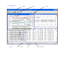
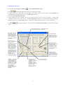
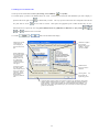
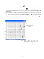
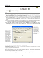
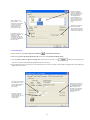
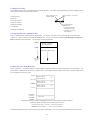
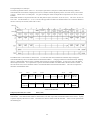
USER’S MANUAL
MagicProcessorK
V3.0
I.O.Technic Co., Ltd.
28-19 Minami-tsukushino 2-chome, Machida City, Tokyo,194-0002 Japan
Phone 81-42-796-3933
2006/1
CONTENTS
1-1.Introduction
2
1-2. Each part name
3
2-1.How to install MagicProcessor
4
2-2.Method for Activating MagicProcessor
4
3-1.Raw Data Graph
5
3-2.Editing Raw Data Graph
6
3-3.Numeric Values Table for Raw Data
7
3-4.Modifying Raw Data
7
3-5.Processed Result Graph
8
3-6.Editing Processed Result Graph
9
3-7.Numeric Value Table for Processed Results
10
3-8.Modifying Processed Results
10
3-9.Editing Processed Result Table
11
3-10.Power Spectrum
12
4-1.Execute processing
13
4-2.Processing Technique
14
4-3.Processed Result Items
14
4-4.Automatic Processing
15
4-5. Automatic backup
15
5-1.Print
16
5-2.Automatic print
17
6-1.File(Menu)
18
6-2. Editing
19
6-3.View
19
6-4.Processing
20
6-5.Window
21
6-6.Help
21
6-7.Pop-up Menu (Right-button Click Menu)
21
7-1.Paste Table to Excel Cell
22
7-2.Paste Table to Word
22
8-1.MagicProcessor Files
23
8-2.Compressed File (sm***p.k02 Binary File)
23
8-3.Master File (sm***m.k02 Binary File)
23
8-4.Processed Result File (sm***l.k02 Text File)
25
8-5.Text Data File (sm***NNNNa.k02 Text File)
26
1
1-1.Introduction
MagicProcessorK computes and processes data collected from Wave Hunter and KOBANZAME.
heights, wave directions, and current velocities to tabulate or plot the results into tables or graphs.
function to create real-time systems by using telephones or telemeters.
It calculates normal wave
It has also a communications
Processing functions
The software computes the following items on the basis of both hydraulic pressure data (converted to surface wave height by the FFT method) and
wave height data collected using ultrasonic gauges
Wave-height processing items
Wave direction processing items
Current velocity processing items
Meteorological
items
data
processing
Maximum wave height and period, 1/10 of maximum wave height and period, significant wave height and
period, average wave height and period, wave count, water depth, η rms, skewness, Kurtosis, water level,
maximum long-period wave height and period, and significant long-period wave height and period.
Average wave direction by covariance method, main wave direction, average angle of dispersion, directional
concentration factor, and wave peak length parameter.
Average current velocity, average current direction, average E-current velocity, average N-current velocity,
and water temperature.
Maximum instantaneous wind velocity, average wind velocity and direction, atmospheric pressure, and
atmospheric temperature,. Oxygen saturation level, Dissolved oxygen, Salinity
Display function
Offers the capacity for producing beautiful, bold displays of tables and graphs that take full advantage of the Windows interface
(including colors, selection of fonts, and multiple windows). You can display an original table or graph by freely selecting one
from above table.
Print function
You can print tables and graphs by directly taking advantage of Windows print functions (colors, fonts, sheets, selection
between horizontal and vertical print directions, transmission to fax, etc.). Graphs and tables can be copied using the mouse and
pasted on Word or Excel documents.
Building a real-time system (Using
KOBANZAME Explorer)
Using radio telemeters, telephones, or cables, data automatically collected from the Wave Hunter can be processed in real time
every time measurement is completed. The system can be fully automated in every aspect of processing from file management
to printing.
Web watch system
Web watch system can be constructed by using IOTechnic Web Center. We choose neither time nor the place, and can check
observational data of the site. Data monitoring system using Internet can be easily constructed.
2
1-2. Each part name
Scroll bar
Title bar
Menu
Status bar
Tool bar
State display
3
2-1.How to install MagicProcessor
Please click "Setup.exe" in installation CD. Respond to the instruction given by the setup program to install. Please change the
directory of installation destination clicking [Change in directory] button while installing it as follows.
Before: C:¥Program Files¥KOBANZAME30¥
After: C:¥KOBANZAME30¥.
Note 1:Click "OK", if the statement "Setup cannot be continued because some system file in the system is not the latest one" is made.
Click "Yes", if the question "Will you restart the Windows?" is made. Try to setup again, when the Windows has been
restarted.
Note 2:Click "Yes" for the statement "The version of the file being copied is either the former one or the same as that existing in the
system."
Expressing system date and time
MagicProcessorK can express only the date and time shown below.
Modify them if the setting differs from Windows' Set as
follows for "Control panel"-Icon[Regional and Language Options]-Button[Customize…]-Tab[date]-[short date] and Tab[time]-[Time
format].
[Date]-[Short Type]
yy/MM/dd
[Time]-[Time format]
H:mm:ss
2-2.Method for Activating MagicProcessor
Drag and drop the file "C:¥KOBANZAME30¥MK30.EXE" to the Windows desktop to create a shortcut. Launch MagicProcessorK
by double-clicking on this icon.
You may change command options at launch time by following the procedure described below.
If you change the contents of properties tab[Shortcut]-item[Target] for the icon "Shortcut to mk30.exe" created above:
from: "C:¥KOBANZAME30¥MK30.EXE"
to: "C:¥KOBANZAME30¥MK30.EXE" 1,
the PC will start MagicProcessorK with the previous status restored.
The following is an explanation of the command line format:
"Path¥mk30.exe" Flag
Path¥
Specify the name of the directory path where “mk30.exe” is contained.
Mk30.exe
Name of this application's execution file
Command option
Flag Bit0= 1
0
Launches the application with the previous status restored.
Launches the application after initializing it.
Flag Bit1
undefine
Flag Bit2
undefine
Flag Bit3
undefine
Flag Bit4= 1
Automatic backup function ON.
0
Flag Bit2= 1
0
Automatic backup function OFF.
Initializing file write protection ON.
Initializing file write protection OFF.
Example:
For "C:¥KOBANZAME30¥mk30.exe 1
the previous status is restored is when the application is launched.
4
3-1.Raw Data Graph
. This is automatically displayed if the file is opened for the
1.Open the master file (sm***m.k02) with Menu [File-Open]
first time or has previously been opened.
2.A raw data graph can be displayed with Menu [View-Raw data graph]
because it is made into a line by a specified value.
Conditions]
.
Note that the graph looks as if it was not plotted,
The format of a graph can be changed by using Menu [Processing-Set
-Tab[Graph]
Clicking the plotting
point moves this. It
moves jointly with the
list mark in the raw data
list.
A water pressure value measured
with a semi-conductor pressure
gauge. The value after processing
indicates the water level (cm).
Indicates the character string, machine number,
measurement number, and measurement date for [Header
Sentence] of [Print]. This indication can be kept from
appearing, using the initializing file.
The right button click menu command, [F3], or [F4] is convenient for enlarging or reducing a graph.
5
It moves in the display area
of a graph, within the
measurement time. In the
large change it can move by
one minute and in the small
change it moves by one
sample. Check the amount
of movement with the status
bar. Plot graphs again
with [Redisplay] of the
click menu. The list mark
of the raw data list moves
jointly.
3-2.Editing Raw Data Graph
1.Edit with Menu [Processing-Set Conditions]
2.Check
-Tab [Graph-Set Raw Data Graph].
one from [1] to [4] and select raw data to be displayed or printed.
3.For better visibility of the graph, determine the [Y Scale] of each channel. If the data value is unknown, turn [Automatic] ON.
For comparing the waveform in the same scale, turn [Interlock] ON as well.
4.Determine [X Scale: Duration Mes.(Min.)].
5.Turning [Vector] ON plots a sampling value for NE component current velocity on the NE coordinate. It allows visual
confirmation of the locus of a current velocity. Turning [Long period] ON displays a wave generated after long-period filtration.
6.Depending on preference, turn [Overlap] ON/OFF.
7.Click
to display the data again.
Clicking one from [1] to [4] specifies the line color for each channel.
Only the value of [X Scale: Duration Mes.(Min.)] is updated when a change is
made.
Set a desired item to ON. Channels that cannot
be specified are displayed in a light color.
Specifies the line color
for a graph. Click one
from [1] to [4] and D to
display the dialogue box
and select your preferred
color. Clicking the
[Update] button plots the
graph again.
For each channel the
graph scale is made
identical. In this way the
size of waveform can be
compared more easily.
Specifies the Y-axis
scale. It specifies in the
units of hydraulic
pressure (g/cm2), current
velocity (m/sec), and
water level (cm) of an
ultrasonic wave height
gauge. Select one from
the down list or key in a
value. If [Interlock] is
ON, changing and
specifying a value for an
item will change that for
other channels the same
as the value changed and
specified. If
[Automatic] is ON,
changing and specifying
a value will be ignored.
Graphs are stacked and
displayed. Comparison
is made regarding phases
of current velocity and
between waveforms of
hydraulic pressure and of
ultrasonic wave. When
processing is performed
with raw data graph
being displayed,
hydraulic pressure made
into surface wave is
displayed.
When potting a graph,
the Y-axis scale is
determined automatically
in reference to the
measurement. When
[Automatic] is ON, [Y
scale] is ignored even if
it has been set.
Specifies the scale
(minute) from the left
end to the right end of a
graph. Select one from
the down list, or key in a
value (1 to 60 minutes).
Data about N & E
component current
velocities are plotted as
are on the
second-dimensional
coordinate. The wave
direction and current can
be judged visually,
referring to the locus of
the current velocity.
6
Plots waveforms after
long-period filtration.
3-3.Table of Numeric Values for Raw Data
. This is automatically displayed if the file has previously been
1.Open the master file (sm***m.k02) with Menu [File-Open]
opened.
2.The raw data table can be displayed by clicking [View-Numeric Value Table for Raw Data]
change font and color.
. The format of the table can
Scrolls the table.
It
only scrolls the table.
The list mark and cursor
do not move.
Indicates the value
of a graph mark. It
moves jointly when
clicking on the plot
point of a graph.
Fonts and background
colors can be changed.
3-4.Modifying Raw Data
Raw data is modified directly to rewrite the data file. Since the original data cannot be restored, make sure to have a copy of the
original file prior to start of modifications. Save the data using Menu [File-Save As], rather than using [Save by Overwriting] to
create an identical file having a different name, which may be freely modified.
7
3-5.Processed Result Graph
. Check the name of the processed result file with the title bar
1.Open the master file (sm***m.k02) with Menu [File - Open]
on the main window.
If no file is available, newly create a data file by processing as specified in [4-1. Execute Processing]
.
If the file has already been open, a data file will appear automatically.
2.A processed data table can be displayed with Menu [View - Processing Results Graph]
with Menu [Processing - Set Conditions]
.
The graph format can be changed
- Tab [Graph].
Indicates the character string, machine number,
measurement number, and measurement date for [Header
Sentence] of [Print]. This indication can be kept from
appearing, using the initializing file.
Moves when the plot
point is clicked. It
moves jointly with the
list mark of the
processed result table.
A processed result displays
data (average wave direction,
main wave direction, current
direction, and wind direction)
indicating directions. The
top of arrows is in magnetic
north. The current flows to
the direction to which the
arrows are pointing.
The right button click menu command, [F3], or [F4] is convenient for enlarging or reducing a graph.
8
3-6.Editing Processed Result Graph
1.Edit the processed result graph with Menu [Processing-Set Conditions]
-Tab[Graph-Set Processing Result Graph].
2.Select a processed result item to be displayed or printed from [1] to [4] and [D] in the down list
space is selected, its channel is not plotted.
.
If 65th
Do not set a space to Channel [1].
3.Determine the Y-axis scale for each channel. For better visibility of a graph, determine the [Up lim] and [Low lim].
of a result is unknown, set [Auto] to ON.
If the value
4.Determine the [X Scale (day)] and [X Lines].
5.Determine ON/OFF settings for [Mark] and [Value].
channel.
6.Click
As desired, clicking the numbers [1] to [4] specifies the line color for each
to refresh the display.
Specifies the lower limit value for the Y-axis scale of a
graph. Click to select a value from the down list. It
can also be entered using the key. The number of Y-axis
graduations is five. Do not set the same value for the
upper and lower limit values.
Specifies the upper limit value for Y-axis scale of a
graph. Click to select a value from the down list.
Specifies the line color
of a graph. Click one
from 1 to 4 and D to
display the dialogue box
and select a desired
color.
Clicking
[Update] plots the graph
again.
The Y-axis scale is
automatically determined
by calculating with a
measurement. When
this is ON, the [Low.
lim] or [Up. lim] that has
been set will be ignored.
Marks Marks [o] and [ ]
will be drawn for
surrounding the plot
point.
Displays the value of the
point right by the plotted
point.
A processed result
displays data (average
wave direction, main
wave direction, current
direction, and wind
direction) indicating
directions. Items with
16 azimuth expressions
cannot be selected. So,
select items displayed
with degrees.
Determines the number of measurement days
from the left end to right end of a graph.
Select one from the down list, or key in a
value. The value having decimal point in the
down list is used for specifying a scale by
time. Changing the value of [X scale]
changes the value of [X Lines] that is
considered appropriate.
Specifies the number of X-axis graduations to be plotted
on a graph. Changing the value of [X scale] changes the
value of [X Lines] that is considered appropriate.
9
3-7.Numeric Value Table for Processed Results
1.Open the master file (sm***m.k02) with Menu [File-Open]
. Check the processed resutl file name, using the title bar on the
main window. When the file is not available, newly create it by processing as specified in [4.1. Execute Processing].
file is opened for the first time or has already been open, it will appear automatically.
2.Use Menu [View-Numeric Value Table for Processing Results]
When the
to display the numeric value table for processed results.
The table format can be changed with Menu [Processing-Set Conditions]
-Tab[Table].
Scrolls the table.
The list mark or
cursor does not
move.
Indicates the value
of a processed result
for the graph mark.
3-8.Modifying Processed Results
Replacing unnecessary results with error values
1.Display a processed result table and move the cursor to the line you want to modify (by clicking the left mouse button). Modify
the line using Menu [File - Save by Overwriting Line Error Value]. The displayed value is shown as " ----" and the point
disappears from the processed result graph. You can perform the equivalent action using the right-click Menu [File - Save by
Overwriting Line Error Value]. Function key F2 may also be used for convenience.
2.To restore the original line overwritten by error values, move the cursor to that line and execute the right-click Menu
[Reprocessing].
Modifying abnormal values in a processed result graph
1.Click the plot point of the abnormal value in the processed result graph. As the graph mark moves, the list mark of the processed
result table will point to the corresponding processed result. Move the cursor to the abnormal value of the processed result table
and correct the value. To modify more than one point, key in the correct values in the same way. Use the same format for the
values. Delete the old values and restore the table back to its original format, confirming that it won't be displaced. Use Menu d
[File - Save by Overwriting] to modify the values. The processed results graph will appear again, this time with modified values.
You can perform the equivalent action using the right mouse button Menu [Save by Overwriting].
2.To restore an original value that was modified, move the cursor to that line and execute the right-click Menu [Reprocessing].
10
3-9.Editing Processed Result Table
1.Edit a processed result table with Menu [Processing - Set Conditions]
-Tab [Table].
2.Click and specify a position to be added from the list at left. Select the processed result items ResultFile you want to display or
print from the list at right. Click
of a print sheet or screen.
to add an item you want.
for two items is secured.
The very top item in the list at left corresponds to the left end
Insert spaces at appropriate spots to make the table easy to view.
Add blank lines as required by also using [Insert Blank Line Every [BB] Hour, in Reference to [AA] Time].
, and
,
buttons are also convenient.
3.Click the
or
button to refresh the table display.
Select the processed
result items you
want to display or
print from the list at
left.
Add items at right to
the list at left.
Replace items at left
or delete. Spaces
can also be added.
When updated with
this item kept [OFF],
a processed result
(significant wave
height, water level,
etc.) obtained by
calculation with
water pressure data
will appear.
Standard items:
Items are made as
standard.
For better visibility
of a table, blank
lines will be inserted
into it at an interval
specified. Time
will be adjusted for
blank lines by
specifying reference
time.
Clearing items: All
the 24 items are
replaced by spaces.
Click and update graphs or tables when setting conditions are changed for [Processing],
[Table], [Graph], [Communicate], or [Print]. Clicking [OK] also performs updating
graphs or tables. When [OK] is clicked, the window disappears after updating. To
always show the window [Set Conditions] at your nearest side, click the larger image
(picture) in the window.
11
,
3-10.Power Spectrum
1.Open the master file (sm***m.k02) with Menu [File-Open]
.
If the file has previously been open, it will appear
automatically.
2.The power spectrum can be displayed with Menu [View-Power Spectrum]
For better visibility of a graph, select Number of
pieces of power spectrum data and Number of filtration repetitions appropriately, using Menu [Processing-Set Conditions]
-Tab [Processing].
3.This is a power spectrum for raw data of water pressure, E-component current velocity, N-component current velocity, and water
level.
When a water pressure is displayed with Menu [Processing-Execute Display]
water pressure as is.
, the power spectrum indicates the
If the power spectrum is displayed after processing with Menu [Processing-Execute Processing]
spectrum indicates a water level which is theoretically compensated for.
Water pressure (water
level converted into
surface wave after
processing)
Indicates the character string, machine number,
measurement number, and measurement date for [Header
Sentence] of [Print]. This indication can be kept from
appearing, using the initializing file.
12
, the
4-1.Execute processing
. This displays the raw data graph. Check and
1.Open the master file (sm***m.k02) to be processed, using Menu [File-Open]
confirm the data in the raw data graph displayed. Note that land data appears linear as if nothing has been plotted. If necessary,
check and confirm the raw data table by displaying the raw data table with Menu [View-Numeric Value Table for Raw Data]
.
When data checking is complete, move the scroll bar to the left end and restore the first measurement number.
2.Make a setting in Menu [Processing-Set Conditions]
-Tab [Processing] .
.
3.Execute processing once with Menu [Processing-Execute Processing]
For reference, see the explanation below.
A processed results table ResultList will appear.
If necessary, also display a graph, using Menu [View-Processed Results Graph]
and the raw data graph to reduce processing time.
Arrange the window by
of the tool bar Toolbar, using the last-recorded
4.Set the number of measurements to be processed in the list box
measurement number at Status bar Statusbar as a guide.
cancelled by clicking
.. If not necessary, close the raw data table
Clicking
initiates continuous processing.
The processing may be
. Processing needs to be done only once. The processed results table and processed results graph can be
displayed or printed again later as many times as desired in different formats, using the processed results file.
This is required for the
expression used for
converting water
pressure fluctuations into
water level fluctuations.
The water pressure
gauge is mounted on the
lid for the Wave Hunter.
Specifies a deviation angle between due north and
magnetic north, in the counterclockwise direction. For
Tokyo it is 6 A processed result obtained when zero
has been specified is one obtained in the direction
relative to magnetic north.
Sets a zero compensation value for a
component current velocity. When
zero calibration is locally made for a
current velocity, its value is entered as
the compensation value.
The smaller the specified
value is, the better the
noise filter effect
becomes. Note that
excessively large values
will deform even the
original waveform.
Water level relative to a
certain index can be
displayed by reducing
this compensation value
from water depth.
Water level = Water
depth - Water level
compensation value
If even normal data is
deformed due to an
excessive noise filtration
effect, lower the level
value and increase the
number of frequencies to
specify in this box.
Specifies a cut-off period
by second for the
long-period wave filter.
Check the waveform
after filtration with the
power spectrum graph
and raw data graph.
Specifies the number of
pieces of data when a
spectrum graph is
plotted. "0" represents all
pieces of data for one
measurement. The
number of pieces of data
is always a value of 2
raised to the Nth power.
Set to OFF for data of
WH99 or 94. Set to
ON only when
processing data of
former types of Wave
Hunter orΣ.
In observation of coastal wave directions, correct indexes are
given to calculation of the main wave direction by specifying
the range of directions on the ocean side along a coastal line
where the Wave Hunter is installed, presuming there will be no
waves coming from the land. Make sure that angles will
always be specified in the clockwise direction relative to
magnetic north. In the case of an illustration shown at right,
make it 34 to 160. When an angle is specified like 330 to 40
over magnetic north, specify it in the clockwise direction.
Specifies the number of
repetitions of filtration
for smoothing the power
spectrum graph.
N
A(34ﾟ)
B(160ﾟ)
W
E
S
13
If the S/N ratio of a signal is poor
(waves are small due to the water depth
of a spot installed with the instrument
being shallow), errors will become
greater to result in poor calculation of
wave direction. If significant wave
heights are lower than the judged value,
the wave direction will be displayed
with an error value.
4-2.Processing Technique
1.To reduce processing time, close all windows before starting continuous processing, displaying tables and graphs only when
processing is complete.
2.If processing starts from a measurement number midway, the portion demarcated by the first measurement number up to the
number immediately preceding this measurement number will be filled with provisional processed results. To process the
unprocessed portion, use the scroll bar to move the measuring number.
3.Reprocessing method:
Click in the processed results table and move the cursor to the desired measurement number. Click
or the right mouse button Menu [Reprocess].
In a processed result graph, click the plot point to specify the measurement number
4.Delete unnecessary processed results (such as data on a land), referring to [3-8. Modifying Processed Results].
4-3.Processed Result Items
Listing of Processed Result Items
01:
05: Dissolved oxygen(mg/l)
09: Max. wave height
(Hydraulic pressure ,m)
13: Significant wave height(m)
17: Standard deviation (ηrms)
21: Salinity(‰)
25: Mean direction (°)
29:
33: Average current velocity (m/sec)
37: Max. long-period wave height (m)
41: Average wind velocity (m/sec)
45: Air temperature (°C)
49: Max. wave height (Ultrasonic, m)
53: Significant wave height (m)
57: Standard deviation (ηrms)
61:
02: Year
06: Oxygen saturation level(%)
10: Max. wave period (sec)
03: Month: Day
07: Measurement number
11: 1/10 of max. wave height (m)
14: Significant wave period (sec)
15: mean wave height (m)
18: Skewness
19: Kurtosis
22: Water level (m)
23: E-component current velocity (m/s)
26: Same as left(16 azimuth expressions) 27: Principal direction (°)
30: Average dispersion angle(°)
31: Directional concentration factor (γ')
34: Average current direction (°)
35: Same as left (16 azimuth expressions)
38: Max. wave period (s)
39: Long-period significant wave height (m)
42: Average wind direction(°)
43: Same as left (16 azimuth expressions)
46: Max. instantaneous wind velocity (sec) 47: Max. instantaneous wind direction(°)
50: Max. wave period (sec)
51: 1/10 of max. wave height (m)
54: Significant wave period (sec)
55: Mean wave height (m)
58: Skewness
59: Kurtosis
62: Water level (m)
63:
14
04: Hour: Minute
08:
12:1/10 of max. wave period
16: mean wave period (sec)
20: Wave count
24: N-component current velocity
28:Same as left (16 azimuth expressions)
32: Long crestedness parameter (γ)
36: Water temperature (°C)
40: Long-period significant wave period (s)
44: Atmospheric pressure (hPa)
48:Same as left (16 azimuth expressions)
52: 1/10 of max. wave period (sec)
56: Mean wave period (sec)
60: Wave count
64:
4-4.Automatic Processing
1.Make a setting in Menu [Processing - Set Conditions]
-Tab [Auto Processing].
2.Make settings in [Next Processing Time] and [Processing Interval] of [Set Automatic Processing] on the same tab in
consideration of measurement finish time and data collection time of the Wave Hunter. Normally, an appropriate time length to
be specified for a real-time system is about five minutes later after completion of measurement. Specify [Master File] with a
master file (sm***m.k02).
3.Turn on [Automatic Processing] and click
. The status bar displays time as far as in second to indicate that the
automatic function is activated.
4.Keep waiting util the processing time comes.
table or graph.
When the time comes, the system will execute processing to update and display a
Specifies time to execute
processing next. It will
specify a little later time
(five minutes later after
completion of
measurement) where
data is automatically
collected and written in a
file.
This item is set to ON for
executing automatic data
collection. Time on the
status bar will be
displayed by seconds and
notifies the automatic
function is operating
Specifies a automatic
processing interval
(minute). Normally, it
will be equal to the value
of a measurement
interval.
The processed master file is specified. Two or more
After automatic processing ends of specified day
master files can be registered.
(Monday), the data file is backed up.
4-5. Automatic backup
Tab [Auto Processing]. item[Automatic backup] is checked. After the first automatic processing on Monday is ended, “smNNN"
folder is made in current folder usually. “BYYYYMMDDHH" folder is made under that, and the file related to “smNNN-.k02" is
copied.
15
5-1.Print
First display a file.
1.To display, open the master file (sm***m.k02)or processed result file (sm***l.k02)DataFile with Menu [File - Open]
2.Select a table or graph to be printed by clicking on
Conditions]
,
,
,
, and
.
.
Edit with Menu [Processing - Set
-Tab [Table] or -Tab [Graph].
Print.
3.Select and key in the [Header Sentence]. Machine number and measurement date and time will be added automatically. Determine
longitudinal and lateral directions of a sheet with [Select Paper]. [Number of Mes. per Page] is effective for [Numerical Value
Table for Processing Results]. Specify the number of measurement frequencies.
4.If a graph is selected, all the parts of the graph will unconditionally be printed. For the window command [Numerical Value
Table for Processing Results], bring the cursor to the line of measurement date and time that is placed to the head of a sheet, and
perform and check test printing with Menu [File-Print]. If letters are printed out of the sheet, adjust printing with different sizes
of fonts.
5.If you want to print part of a table or graph, drag the part to be printed using the mouse, and select that part after flipping to display
it. To print one page, place the cursor to the line of measurement date and time that needs to be put ahead of a sheet.
6.Define [Print range], [Copies] and [Printer] with the menu command [File-Print], and then click [OK] to start printing.
Printing will take a lot of time if it is for a large volume or complicated graph. To print all parts of a table or graph, select [All]
with [Print range].
Specifies a header
sentence entered in a
processed result table,
processed result graph,
or raw data graph. This
column may be left
unwritten. Using the
initializing file, the
machine number,
number of measurement
frequencies, and date and
time for the header can
be unrevealed.
Specifies the number of
measurement frequencies
per page at a time a
processed result table is
printed. The number of
lines to be printed is
determined by sheet size,
longitudinal and lateral
directions of a sheet, and
font size. When
specifying the number of
measurement
frequencies, make it an
easy-to-count one, such
as that for a day or two
days. In printing where
[All] is selected, the
number of fractional
measurement frequencies
for the fist page will be
adjusted automatically.
Other tables or graphs can also be printed as explained above. Note the following:
For Processing Result Graph:
Adjust the font size if a graph is displayed unevenly. A lot of time will be required to display a complicated graph. The line size
or mark size can be adjusted with the initializing file.
For Raw Data Table:
If you want to print part of a table or graph, drag the part to be printed using the mouse, and select that part after flipping to display it.
Printing will not be performed only if the cursor is placed to the part you want to print. Note that printing the amount of one
measurement of raw data will make the number of pages too large.
For Raw Data Graph:
Note that if data values are constant the graph shown will be linear, which may look as if no graph was plotted.
16
Indicates a standard
printer for Windows.
Select [Longitudinal] for
[Sheet] in [Property].
The longitudinal or
lateral direction of a
sheet is specified in the
print format window as
shown in the previous
page.
This is effective for
printing a table. The
whole part of a table that
is focused on will be
printed. Be cautious
when handling the
window for raw data.
Specifies the number of
sheets to be printed.
This cannot be specified
if the printer driver does
not have such a function.
Prints only the part of a
table that is selected. If
nothing has been
selected for a table, the
whole part of a page will
be printed in reference to
the cursor line.
5-2.Automatic print
1.Make a setting in Menu [Processing-Set Conditions]
-Tab[Print-Print Format].
2.Make setting [Next Print Time],[Print Interval] on the same Tab [Setting Automatic Print].
3.Turn on [Print a Table] and [Print a Graph]. Both of them can be checked. Click
. The status bar displays time
as far as in second to indicate that the automatic function is activated.
4.Keep waiting until the processing time comes. When the time comes, the system will print tables and graphs. Raw data tables and
graphs cannot be printed.
Specifies time to execute
processing next. It will
specify a little later time
after completion of
processing)
This item is set to ON for
executing automatic prit
of [Table]and [Grapsh].
Both of them can be
checked. Click [Update].
Time on the status bar
will be displayed by
seconds
Specifies a automatic
processing interval
(minute).Set this item to
finish printing at
required time.
17
6-1.File(Menu)
Ctl + O
Open
The following four types of file can be opened. For a standard file, specifying a master file will automatically open a
processed result file too. On the other hand, specifying a processed result file will automatically open a master file. Files
having an arbitrary name can also be opened. A file having a name with a character “L” or “S” given before an extension is
regarded as a result file. The title bar in a window will indicate the name of a file in use.
Master file (sm***m.k02), Temporary data file (sm***t.k02), Process result file (sm***l.k02), and Temporary result file
(sm***s.k02)
Close
This command will save a state of MagicProcessor, close the file, and clear the display.
Initialize
F9
The setting condition of MagicProcessorK is initialized and displayed. The message to request the permission of initialization is
displayed. When initializing it, [yes] is clicked.
Save by Overwrite
Right-button click menu
Ctl + S
A master file will be overwritten with a value in a raw data table corrected. The correction unit of raw data is for one
measurement. Save it before displaying the next measurement data. If a processed result table is corrected, a processed result
file will be overwritten with a value in the table. The correction unit of a processed result file is for a file. Overwriting
should be saved as frequently as possible, however it can be saved whenever desired.
Save by Overwriting Line Error Values
Right-button click Menu
F2
This command overwrites an unnecessary part (overwrites one measurement with error values for data that makes a table or
graph hard to view, such as land data) of a processed result file with error values for each measurement. Use this function to
organize a table or graph to make it easier to view.
Save As
This command stores a modified value table under a different name. Note that raw data can be modified one measurement unit
at a time. Since the contents of the data file are rewritten when you execute [Save by Overwriting], we recommend creating a
copy (having the same content but a different name) of the file using the [Save As] command. Processed results files can be
recalculated and modified as many times as desired, as long as the relevant data file exists.
Back-up
The “sm***" folder is made in a current folder. The “BYYYYMMDDHH" folder is made under that. All data files
(sm***?.k02) are copied.
File Move
The “sm***" folder is made in a current folder. The “BYYYYMMDDHH" folder is made under that. All data files
(sm***?.k02) are moved.
Print See Page 16.
Decompress Compressed File
1.Open a compressed file (sm***p.k02) with Menu [File-Decompress Compressed File]. The decompressing condition will
be indicated on the status bar and a master file will be created. There will appear a message “Specify Measurement Number of
File Decompressed”. Measurement number of data will be specified in the following cases:
A.When the measurement number of data recorded is known
B.When decompressing will partially be done again
2.If the measurement number is unknown, click [OK] to start decompressing.
Converting Convert into Text Data File
To execute data conversion, click Menu [File-Convert into Text Data File]. The converting state will be indicated in the
header information. Data will be converted into a master file (sm***m.k02) and a text data file (sm***NNNNa.k02). For
each file, an inquiry will be made regarding the frequency of measurement to be recorded, which should be keyed in with
half-size characters. When the number 1 is entered, a file will be created for every measurement. To collect in one text data
file, specify the number 99999. NNNN of sm***NNNNa.k02 is a measurement number recorded in the beginning of the file.
It will be three to four times the size of a master file.
18
End MagicProcessor
A current status will be saved and the application will be terminated.
6-2. Editing
Right-button click menu
Zoom
F4
X axis: X axis will be reduced to plot a graph again, in reference to the graph mark.
Y axis: The Y-axis direction will be enlarged to plot a graph again.
It will reduce the graduation.
Right-button click menu F3
Reduce
X axis: X axis will be reduced to plot a graph again, in reference to the graph mark.
Y axis: The Y-axis direction will be reduced to plot a graph again. It will enlarge the graduation.
Ctrl+X
Cut
A selected part will be cut off onto the clipboard.
graph.
Copy
Right-button click menu
This will be used for correcting a raw data table.
It cannot be used for a
Ctrl + C
If a graph window has been selected, the whole window will be copied onto the clipboard. For a table, the selected part will be
copied onto the clipboard. Using the menu command [Edit-Select All] will permit selecting the whole of a graph (the header
part not included). This function will be used for correction. It can also be used for pasting a table or graph in a Word or
Excel document.
Paste
Ctrl + V
This function pastes a content written on the clipboard in a table.
graph.
It will be used for correction, but cannot be pasted into a
Font
This is for specifying a font used for a table or graph. Fonts to be used for a table have restrictions as follows.
a graph will be displayed as specified.
Fonts used for
1.It is not possible to use proportional fonts such as MSP Gothic font represented by P.
2.Depending on the size of characters, the alignment of a table could be in disorder with a true type font (such as MS Ming),
even if it may not be a proportional one.
3.Numeric values in a table cannot be specified with a font (character) color. The header part can be specified with a font
color.
Background Color
This is to specify a background color for a table or graph. Depending on the system, 16 basic colors and Windows system
colors could only be used for the background color of a table. Resembling these colors, there are other intermediate 16 basic
colors. The background color of a graph will be displayed as specified.
Select All
Except for the header part, all the texts in the window will be selected.
This is used for correction of a table.
6-3.View
Redisplay
Right-button click menu
This command is used for displaying a measurement number linked with a processed result graph at the time the measurement
number is moved by the cursor or scroll bar in a processed result table. They will not be redisplayed if existing within the
moving point (checked with the graph mark). It will also be used for displaying a data number linked with a raw data graph
when the data number is moved by cursor in a raw data table or by the scroll bar in the raw data graph. The measurement
number will not be added with 1, as indicated by Menu [Processing-Executing Display]
See Page 10.
Numeric value table for Processing Result
See Page 8.
Processing result graph
Numeric value table for raw data
Raw data graph
See Page 7
See Page 5.
19
.
See Page 12.
Power spectrum
Tool bar
This will turn ON/OFF the display of the tool bar.
Status bar
Scroll bar
This will turn ON/OFF the display of the scroll bar.
Machine number: This is a specific number used for
identifying an instrument. The only one piece of sample
data acquired by the Wave Hunter will be identified with
three numbers the machine number, measurement number,
and data number. The machine number is the first element
used for identifying data, which is a fundamental element
with which MagicProcessor will create a file name.
Measurement number:
This is a value which
the Wave Hunter has
accumulated by 1 for
each measurement.
This will indicate
information about
MagicProcessor’s
operation.
Data number: The
sample data number
assigned during
measurement time.
The value in the
brackets indicates a
lapse time after start
of measurement.
This will indicate time
on a personal computer.
Up to seconds will be
indicated if the
automatic function has
been set.
Measurement start
date
Measurement start
time
This will scroll a measurement number by clicking the
mouse or dragging the pointer. The measurement
number will not be shown even if it may be moved. To
show it, click
or use the right-click menu command
[Redisplay].
6-4.Processing
Execute Display
This command is for displaying data of the next measurement number. To display continuously, select from the down-list in
the list box on the tool bar or key in a value and click The specified number of pieces of measurement data will be displayed
continuously. To cancel displaying, click
.
Execute Reverse Display
This command is for displaying data of a measurement number immediately before the current one.
select from the down-list in the list box on the tool bar or key in a value and click
measurement data will be displayed continuously in a reverse direction.
.
To dsiplay continuously,
The specified number of pieces of
To cancel displaying, click
.
Execute Processing
To specify, select the number of measurement frequencies in the down-list in the list box on the tool bar or key in a value.
Click
to execute processing continuously.
Cancel
This command is for canceling operation in the middle.
Set Conditions
See Page other .
6-5.Window
Display Overlapping Window
20
Windows will be overlapped to display.
Display Tiled windows
Windows will be placed in a lateral direction to display.
Display Vertically-Tiled Window
Windows will be placed in a longitudinal direction to display.
Save Status
It controls by specifying the command line option. The check adheres when the state of MagicProcessor is protected, and it
becomes effective. The check can temporarily release protection by removing by clicking. The state at that time is preserved in
initialization file (mk30i.ini) when the setting is changed after it releases it, and it clicks again. When [Save Status] is not
specified by the command line option, it becomes invalid and it is not possible to operate it.
6-6.Help
Find Topic
This command is to display Help for the application.
Version Information
This command is to display Version Information for the application.
6-7.Pop-up Menu (Right-button Click Menu)
Redisplay
This command is used for displaying a measurement number linked with a processed result graph at the time the measurement
number is moved by the cursor or scroll bar in a processed result table. They will not be redisplayed if existing within the
moving point (checked with the graph mark).
Zoom
X axis: X axis will be enlarged to plot a graph again, in reference to the graph mark.
Y axis: A graph in the Y-axis direction will be enlarged to plot it again.
This command will reduce the graduation.
Reduce
X axis: X axis will be reduced to plot a graph again, in reference to the graph mark.
Y axis: A graph in the Y-axis direction will be reduced to plot it again. This command will enlarge the graduation.
Reprocessing
This command is for processing only data of specified measurement numbers. The graph position will not be changed if
processed results of those measurement numbers are displayed in a processed result graph. This is a useful command for
restoring values modified for processed results.
Set Conditions See Page other.
Save by Overwriting
Ctrl + S
This command overwrites a master file with the values of a modified raw data table. The raw data is modified in a unit of one
measurement at a time. Save the data before displaying data for the next measurement. If modification is made on a
processed result table, the command will overwrite the processed result file with the values found in that table. Processed
result files are modified in a unit of one file at a time.
Save by Overwriting Line Error Values
F2
This command overwrites an unnecessary part (data that makes a table or graph hard to view, such as land data) of a processed
result file with error values for each measurement. Use this function to organize a table or graph to make it easier to view.
Copy
Ctrl + C
When a graph window is selected, this command copies the whole window to the clipboard. If the object selected is a table,
the command copies the part of the table that is selected to the clipboard. Select the entire table (except for the header) using
the menu command [Edit - Select All]. This command is used to make modifications and paste a table or graph into a Word or
Excel document.
Help
This command is to display Help for the application.
21
7-1.Paste Table to Excel Cell
Pasting a table to the cell
1.To insert a table into an Excel cell, use the files “sm22g.txt”, “sm23g.txt” and “sm24g.txt” of the directory containing “mk30.exe”.
files “sm22g.txt” contains a raw data table and “sm23g.txt” a processed results table, and these tables are loaded into an Excel cell.
2.Select and open “sm22g.txt” with the Excel menu command [File - Open]. Select [Data Format] - [Break with Comma and
Tab...] or [Left or Right by Space …] with [Text File Wizard] and then click [Next].
3.Adjust and optimize the line breaking and click [Next]. Load the values into the cell by [Complete].
by deleting unnecessary lines.
Shape the format properly
Pasting a table
1.This procedure is the same as using the ordinary Windows “Copy” and “Paste” function. With the mouse, drag and select the part
of a table you want to copy and select [Edit - Copy].
2.Move the cursor to the part of Excel where the table will be pasted. Then, select [Pasting Format] – Bit Map (DIB) in the [Edit
- Paste by Selecting Format] Excel menu command and paste it. In this case, the data will be pasted in a text format.
Pasting a graph
1.Click and select the window of the graph that will be copied.
Then, copy it with the [Edit - Copy] menu command.
2.Move the cursor to the part of Excel where the graph will be pasted.
- Paste by Selecting Format] Excel menu command and paste it.
Then, select [Pasting Format] - Bit Map (DIB) in the [Edit
Note: If you have difficulties pasting data, open “Clipboard” before copying, clear its contents with [Edit - Delete], then copy.
7-2.Paste Table to Word
Pasting a table
1.This procedure is the same as using the ordinary Windows “Copy” and “Paste” function. With the mouse, drag and select the part
of a table you want to copy and select [Edit - Copy].
2.Move the cursor to the part of Word where the table will be pasted. Then, select [Pasting Format] – Bit Map (DIB) in the [Edit
- Paste by Selecting Format] Word menu command and paste it.
Pasting a graph
1.Click and select the window of the graph that will be copied.
Then, copy it with the [Edit - Copy] menu command.
2.Move the cursor to the part of Word where the graph will be pasted.
- Paste by Selecting Format] Word menu command and paste it.
Then, select [Pasting Format] - Bit Map (DIB) in the [Edit
Note:If you have difficulties pasting data, open “Clipboard” before copying, clear its contents with [Edit - Delete], then copy.
22
8-1.MagicProcessor Files
Place MagicProcessor files in a current directory which has mk30.exe.
can be given according to the specification below.
The name of a file automatically created by MagicProcessor
Lower three digits of a
machine number
Compressed file
These characters are always
used.
Master file
Processed result file
SM***M.k02
Temporary data file
P:Compressed file
M:Master file
L:Processed result file
T:Temporary data file
S:Temporary result file
A:Text data file
Temporary result file
Text data file
Former Wave Hunter file
8-2.Compressed File (sm***p.k02 Binary File)
This is a compressed file collected from the Wave Hunter. Its structure is as below, where the memory file on the main unit is
copied as is. This file cannot be used without decompression. To use it, decompress with Menu [File-Decompress Compressed
File] function and create a master file. Pointer region for each measurement
000000
Pointer region for
each measurement
010000
Compressed data region
Address
inside of
file
8-3.Master File (sm***m.k02 Binary File)
This is a binary file. It normally contains raw data and data is stored in the order of measurement number 1 as shown below. The
tail of the file is suffixed with 65536 bytes of address table. In the address table the address values each of which is added with 1
are recorded by the unit of four bytes.
000000
Header + data of
measurement No. 1
(X)
Header + data of
measurement No. 2
(X)
Header + data of
measurement No. 3
(X)
AAAAAA
BBBBBB
CCCCCC
End Address
-65536byte
Adress table
End Address
CCCCCC
Measurement time of 20 minutes, sampling interval of 0.5s and conditions of three parameters
(hydraulic pressure, E current velocity, and N current velocity)
AAAAAA=(FIX((2400×3+12)÷512)+1)×1024=15360=003C00
BBBBBB=3C00×2=007800
CCCCCC=3C00×3=00B400
The following illustration shows the file structure for a single measurement.
23
The size of a single measurement file will always be
an integral multiple of 1,024 bytes.
The following illustration shows 1,024 x 15 = 15,360 bytes (equivalent to 7,680 pieces of data) under the following conditions:
measurement time of 20 minutes, sampling interval of 0.5s, and three elements (hydraulic pressure, E current velocity, and N current
velocity). The file stores 7,212 data points. Any part exceeding the volume of sample data is composed of error values (-32,768 =
8,000H).
Both header and data are expressed in the ratio one data point/two bytes (value from -32,768 to 32,767). The value -32,768 is an
error value. For data numbers 6, 7, 9, 10, 11, and 12, both upper and lower data in the illustration below are recorded for headers in
the ratio of one byte to one data (values from 0 to 255).
Data Number
Header
Data
Elements of
Measurement
Average
azimuth
Hydraulic
pressure
2
Average water
temperature
E current
velocity
2
Machine
number
/Year
Voltage
/Number of
channels
Measurement
number
N current
velocity
2
Hydraulic
pressure
3
E current
velocity
3
Measurement Measurement
time/
parameters
Measuring interval
1 and 2
N current
velocity
3
Minute
/Hour
Day
/Month
Hydraulic
pressure
4
E current
velocity
4
N current
velocity
4
Hydraulic
pressure
1
E current
velocity
1
N current
velocity
1
Hydraulic
pressure
5
E current
velocity
5
N current
velocity
5
Hydraulic
pressure
8
E current
velocity
8
N current
velocity
8
Hydraulic
pressure
2397
E current
velocity
2397
N current
velocity
2397
Hydraulic
pressure
2400
E current
velocity
2400
N current
velocity
2400
The address table is in the structure as shown below. In a real-time observation, measurement conditions may be changed or
measurement data may not be recorded from that of measurement number 1. Changing conditions for measurement time, sampling
interval, or measurement item will specify a random volume of data for a single measurement. In such a case, refer to the address
table and process the data. If 0 is specified for a specific measurement number of an address table, data has not been recorded. If
the value can be read, it will be an address which is recorded with data for that measurement number. The value is composed of
that of the recorded address and 1.
-65536
-65532
Max.Mes.
number
-65528
Mes. No1
Data adrs.
-65524
-65512
Mes. No2
Data adrs.
-65508
Mes. No6
Data adrs.
Mes. No71
Data adrs.
No16376
Data adrs
-32
Last Mes.
number
-28
-4
File End
Address Table Structure
Temporary Data File (sm***t.k02
Binary File)
The temporary data file sm***t.k02 stores (N=2 is a default value) raw data from those of the latest measurement number to past Nth
measurement. If the measurement number is smaller than N, raw data of up to that measurement number will be stored. It partly
copies the temporary data file sm***t.k02. This function is useful to obtain on-line the latest data. Value N can be specified with
the initializing file.
24
8-4.Processed Result File (sm***l.k02
Text File)
This is a text file containing processed results calculated by MagicProcessor. It can be loaded as is, using a text editor or
spreadsheet software. Its format is as shown below. In each item, processed results below will be entered.
Processed Result Format (392 characters/Result of a single measurement)
Each item consists of a 5-digit numeric value “#####” and a comma “,”. A space character “ “ is inserted next to the comma of
every eighth item, which is repeated up to the 64th item. A carriage return and line feed are appended to the end. A single
measurement has a fixed length of 392 characters.
Item Nos.
Format
01
02
03
04
05
06
07
08
09
#####,#####,#####,#####,#####,#####,#####,#####, #####,#####,
10
………..
63
64
………. #####,#####CRLF
Listing of Processed Result Items
01:
05: Dissolved oxygen(mg/l)
09: Max. wave height
(Hydraulic pressure ,m)
13: Significant wave height(m)
17: Standard deviation (ηrms)
21: Salinity(‰)
25: Average wave
29:
33: Average current velocity (m/sec)
37: Max. long-period wave height (m)
41: Average wind velocity (m/sec)
45: Air temperature (°C)
49: Max. wave height (Ultrasonic, m)
53: Significant wave height (m)
57: Standard deviation (ηrms)
61:
02: Year
06: Oxygen saturation level(%)
10: Max. wave period (sec)
03: Month: Day
07: Measurement number
11: 1/10 of max. wave height (m)
04: Hour: Minute
08:
12:1/10 of max. wave period
14: Significant wave period (sec)
18: Skewness
22: Water level (m)
26: Same as left
30: Average angle(°)
34: Average current direction (°)
38: Max. wave period (s)
42: Average wind direction(°)
46: Max. instantaneous wind velocity (sec)
50: Max. wave period (sec)
54: Significant wave period (sec)
58: Skewness
62: Water level (m)
15: Average wave height (m)
19: Kurtosis
23: E-component current velocity (m/s)
27: Main wave direction (°)
31: Directional concentration factor (γ')
35: Same as left (16 azimuth expressions)
39: Long-period significant wave height (m)
43: Same as left (16 azimuth expressions)
47: Max. instantaneous wind direction(°)
51: 1/10 of max. wave height (m)
55: Average wave height (m)
59: Kurtosis
63:
16: Average wave period (sec)
20: Wave count
24: N-component current velocity
28:Same as left (16 azimuth expressions)
32: Wave-peak length parameter (γ)
36: Water temperature (°C)
40: Long-period significant wave period (s)
44: Atmospheric pressure (hPa)
48:Same as left (16 azimuth expressions)
52: 1/10 of max. wave period (sec)
56: Average wave period (sec)
60: Wave count
64:
Temporary Results File (sm*****s. k02 Text file)
MagicProcessor creates this file in real-time processing. It stores (N=6 is a default value) raw data from those of the latest
measurement number to past Nth measurement. If the measurement number is smaller than N, raw data of up to that measurement
number will be stored. The content of this file can be checked with a text editor. This function is useful to obtain on-line the latest
data. Use this file in a remote system. Further, use this file only for viewing.
25
8-5.Text Data File (sm***NNNNa.k02 Text File)
The description below is a format for a text data file converted with Menu [File-Convert into Text Data File]. The meaning of the
data remains the same. Data will be stored in a file in the order shown below, when collecting 4-channel data during measurement
with a ratio of 10 minutes to 60 minutes (sampling for 0.5 second). NNNN in sm***NNNNa.k02 indicates the head number of
measurement for that file.
Content of Text File
17185,
0,
0, 2226,
Explanations about Text File Items
152,
125
Element Mes. ,
97,
75,
4,
1,
10,
60
Year
1,
55,
55,
16,
7,
1
Parameter1
,Volt
,
.
,Ave.Dir.
,Ave.Temp ,Mach.No
,Number of Ch. ,Mes.number ,Mes.time
,Parameter2 ,minute
,hour
,day
2488,
-3,
11, 2374
Wr.Press.(1)
,E.vel.(1)
,N.Vel.(1)
,Level(1)
2492,
-3,
13, 2377
Wr.Press.(2)
,E.vel.(2)
,N.Vel.(2)
,Level(2)
2495,
-2,
15, 2392
Wr.Press.(3)
,E.vel.(3)
,N.Vel.(3)
,Level(3)
2492,
1,
9, 2394
Wr.Press.(1199),E.vel.(1199) ,N.Vel.(1199),Level(1199)
2491,
3,
8, 2394
Wr.Press.(1200),E.vel.(1200) ,N.Vel.(1200),Level(1200)
2464,
2,
4, 2201,
147,
125
97,
75,
4,
2,
10,
60
65,
55,
55,
17,
7,
1
2459,
3,
5, 2353
2459,
2,
4, 2356
26
,Mes.intvl
,month