Download BugsXLA: Bayes for the Common Man

JSS
Journal of Statistical Software
May 2005, Volume 14, Issue 5.
http://www.jstatsoft.org/
BugsXLA: Bayes for the Common Man
Phil Woodward
Pfizer Global Research and Development
Abstract
The absence of user-friendly software has long been a major obstacle to the routine application of Bayesian methods in business and industry. It will only be through
widespread application of the Bayesian approach to real problems that issues, such as
the use of prior distributions, can be practically resolved in the same way that the choice
of significance levels has been in the classical approach; although most Bayesians would
hope for a much more satisfactory resolution. It is only relatively recently that any general
purpose Bayesian software has been available; by far the most widely used such package
is WinBUGS. Although this software has been designed to enable an extremely wide variety of models to be coded relatively easily, it is unlikely that many will bother to learn
the language and its nuances unless they are already highly motivated to try Bayesian
methods. This paper describes a graphical user interface, programmed by the author,
which facilitates the specification of a wide class of generalised linear mixed models for
analysis using WinBUGS. The program, BugsXLA (v2.1), is an Excel Add-In that not
only allows the user to specify a model as one would in a package such as SAS or S-PLUS,
but also aids the specification of priors and control of the MCMC run itself. Inevitably,
developing a program such as this forces one to think again about such issues as choice of
default priors, parameterisation and assessing convergence. I have tried to adopt currently
perceived good practices, but mainly share my approach so that others can apply it and,
through constructive criticism, play a small part in the ultimate development of the first
Bayesian software package truly useable by the average data analyst.
Keywords: Bayesian analysis, GLMM, Microsoft Excel, graphical user interface, WinBUGS.
1. Introduction
The use of Bayesian methods in academia appears to have increased at an exponential rate
over the last ten to twenty years. There can be little doubt that this is due to the availability
of Markov chain Monte Carlo (MCMC) algorithms to implement such methods that simply
did not exist previously: see Gelfand and Smith (1990), Smith and Roberts (1993) or Tierney
(1994) for details of this approach. The philosophical debate will never go away, but even
2
BugsXLA: Bayes for the Common Man
amongst academics it is the practicality of being able to solve real problems that has greater
influence. Although Bayesian methods are used more today in business and industry than
they were twenty years ago, the increase is nowhere near as marked. I suggest that one of the
barriers to greater use is the unavailability of Bayesian software with a good user interface.
The WinBUGS package of Spiegelhalter, Thomas, Best, and Lunn (2003b) is the most widely
used Bayesian data analysis program. It provides an easy to learn language that allows a
wide variety of models to be specified. Its popularity is probably due to the user not needing
to know very much about the MCMC methods that underpin it, and the fact that it is free!
However, there is inevitably a learning curve barrier associated with any new software that
requires sufficient motivation to overcome. If it were possible to specify a model in a similar
manner to that in SAS, S-PLUS or Genstat, then I believe a much larger number of people
used to working with such programs would try a Bayesian approach.
This paper describes a graphical user interface for WinBUGS that allows a wide class of
generalised linear mixed models (GLMMs) to be specified in a manner familiar to users of
more conventional statistical software. This interface, BugsXLA (v2.1), is a Microsoft Excel
Add-In that is also freely available via the BUGS website: http://www.mrc-bsu.cam.ac.
uk/bugs or direct from http://www.pipshome.freeserve.co.uk/stats; see Appendix B for
instructions on how to download and install the software. Section 2 provides a brief overview
of WinBUGS. Section 3 describes the types of model that can be fitted, and how the model
statement is converted into WinBUGS code. Section 4 explains how priors are specified,
including a graphical tool to help in the elicitation process. Section 5 briefly discusses the
options available for controlling the MCMC run itself. An example is provided in Section 6 to
illustrate how the user interacts with the interface. The remaining functionality not illustrated
by the example is given in Section 7. A few concluding remarks are made in Section 8. Since
segments of WinBUGS code are shown throughout the paper, Appendix A gives a very brief
explanation of the key elements of the language. However, readers not familiar with WinBUGS
may simply wish to skip those parts that discuss the generated code, as it is not necessary to
understand this in order to use BugsXLA.
2. Brief overview of WinBUGS
WinBUGS was developed by Spiegelhalter et al. (2003b) and is an interactive Windows program for Bayesian analysis of complex statistical models using Markov chain Monte Carlo
(MCMC) techniques. In the Bayesian approach all quantities in the model are treated as
random variables, and inferences are made by conditioning on the data to obtain a posterior
distribution for the parameters in the model; see Lee (2004) for an introduction to Bayesian
statistics. The MCMC approach is used to marginalise over the posterior distribution in order
to obtain inferences on the main quantities of interest.
WinBUGS contains a programming language that allows an arbitrarily complex statistical
model to be defined. This code is then compiled into a form suitable for efficient computation,
and a sampler operates on this structure to generate appropriate values of the unknown
quantities in order to feed the MCMC algorithms. Instead of calculating exact or approximate
estimates of the necessary numerical integrals, MCMC generates a stream of simulated values
for each quantity of interest. WinBUGS also has tools to monitor the stream for convergence,
and summarise the accumulated samples.
Journal of Statistical Software
3
3. Specifying the model using BugsXLA
All the major statistical packages used to facilitate classical methods of data analysis allow
the user to specify the model to be fitted by means of a relatively concise model statement. It
is likely that in order to persuade many users of packages such as SAS, S-PLUS and Genstat to
try a Bayesian analysis of their problems, amongst other things, they will need software that
allows models to be specified in a familiar way. BugsXLA uses a very similar set of design
statement symbols as that used in Genstat:
+ : addition of a term
. : interaction between two terms, or a nested term
* : crossing of two terms, i.e., both main effects and the interaction
/ : nesting of second term inside the first
() : grouping; used to determine the order of evaluation for complex models
- : subtraction of a term
@ : only expand terms to order specified, e.g., A*B*C@2 = A*B*C - A.B.C
^ : power term (covariates only), e.g., temp^2 is the quadratic term for temp
These enable quite complex models to be specified very concisely. For example, (A + B)*C is
shorthand for a model with the terms A + B + C + A.C + B.C, while (A + B)/C is a model
with main effects of both A and B, plus a factor C nested within the combination of these
factors. This would be expanded to A + B + A.B.C. Note that although A.B.C is written
exactly the same here, when defining a nested term, as it would be written when defining a
three way interaction term, it may need to be interpreted differently when constructing the
appropriate code to fit the model.
As well as being able to include both independent (“fixed” in classical terminology) and
exchangeable (“random”) effect terms in the model, it is possible to specify covariates. When
specifying the covariate part of the model, the . symbol is used to denote the product of
two covariates. Polynomials can be easily specified by using the @ and ^ operators, e.g.,
(X1*X2*X3*X4)@2 + (X1+X2+X3+X4)^2} would fit all terms up to the second order.
Clearly there is nothing new in developing software that is able to interpret the algebra of a
design statement (see Heiberger 1989, for a thorough explanation of how this can be done).
What is novel is to derive code that fits the specified model using a Bayesian analysis. This
has been achieved by generating the appropriate code that can be run by the WinBUGS
Version 1.4 software package. By utilising the script facility added to this version of the
software, it is then possible to call the program from within Excel, using VBA code, and
retrieve the results after the analysis is complete. All this is possible without the end user
having to know how to use the WinBUGS package at all. There are some dangers in this
approach, which I will briefly discuss in the concluding remarks.
The majority of generalised linear models used in practice are Normal/identity, Poisson/log
or Binomial/logit. These can all be routinely fitted using BugsXLA, the generated WinBUGS
code being of the form:
mu[i] <- Beta0 + ...
Y[i] ~ dnorm(mu[i], tau)
4
BugsXLA: Bayes for the Common Man
or
log(mu[i]) <- Beta0 + ...
Y[i] ~ dpois(mu[i])
or
logit(mu[i]) <- Beta0 + ...
Y[i] ~ dbin(mu[i], N[i])
where log() and logit() are functions, and dnorm(), dpois() and dbin() are distributions intrinsic to WinBUGS corresponding to Normal, Poisson and Binomial distributions
respectively. Note that the BugsXLA user does not need to know how to code in, or run,
WinBUGS at all. BugsXLA creates this code automatically after interpreting a much simpler
model statement as explained above.
By only using link functions that allow the parameters to vary over the whole real line, it
is possible to generalise the code for defining the priors and likelihood contributions of the
parameters.
Software written to use classical methods of statistical analysis converts the list of model terms
to be fitted into an appropriate design matrix. This matrix provides the substrate on which
the numerical algorithms developed to give the parameter estimates are applied. Categorical
factors are converted into dummy variables with constraints to ensure estimable functions are
defined. For example, by default SAS constrains the last level of each main effect to be zero,
while Genstat’s default is to constrain the first level. A different approach has been taken
when generating the data files and code for WinBUGS. Each categorical factor term, be it
main effect or interaction, is stored as a single vector consisting of integers indexing the level
set for each observation. This allows the linear predictor to be specified in WinBUGS code
using the generic statements:
for (j in 1: N.obs) {
for (i in 1: N.X) {
X.row[i, j] <- X.Eff[i, X[j, i]]
}
for (i in 1: N.Z) {
Z.row[i, j] <- Z.Eff[i, Z[j, i]]
}
mu[j] <- Beta0 + sum(X.row[, j]) + sum(Z.row[, j])
}
where N.obs is the number of observations, N.X and N.Z are the number of independent
and exchangeable effects terms respectively, X[,] and Z[,] are matrices made up of the
independent and exchangeable level indexing vectors respectively, X.Eff[,] and Z.eff[,]
are the parameters defining the independent and exchangeable effects respectively, Beta0 is
the constant parameter, and mu[] is the linear predictor in the generalised linear mixed model.
The intrinsic WinBUGS function sum() sums over the missing index of its vector argument.
One of the main tasks underpinning BugsXLA is to convert a model statement of the form (A
Journal of Statistical Software
5
+ B)*C into the appropriate X[,] (“fixed effects”), or Z[,] (“random effects”), design matrix.
Note that each row of these matrices represents a different observation, and each column
represents a different term in the model, with the entries representing the associated factor
level set. X.Eff[,], Z.Eff[,] and Beta0 are what WinBUGS coders refer to as “stochastic
nodes”, representing the statistical parameters of the model, and will need to have priors
specified (see Section 4).
It is equally as simple to write generic code for including covariates. The only additional
issue to consider is the need to centre and scale the covariates, which greatly improves the
performance of the MCMC algorithm as discussed in Gilks and Roberts (1995). The code
required to achieve this in WinBUGS is:
for (i in 1: N.V) {
mean.V[i] <- mean(V[ , i]) ; sd.V[i] <- sd(V[ , i])
Cov.Coeff[i] <- V.Beta[i] / sd.V[i]
for (j in 1: N.obs) {
std.V[j, i] <- (V[j, i] - mean.V[i]) / sd.V[i]
}
mean.Beta[i] <- Cov.Coeff[i]*mean.V[i]
}
alpha <- Beta0 - sum(mean.Beta[])
for (j in 1: N.obs) {
V.row[j] <- inprod(std.V[j, ], V.Beta[] )
mu[j] <- Beta0 + V.row[j]
}
where N.V is the number of covariates, V[,] is a matrix made up of the covariates, std.V[,]
is a matrix of centred and scaled covariates, Cov.Coeff[] and V.Beta[] are the vectors of
regression parameters for the original and scaled covariates respectively, and alpha and Beta0
are the intercept parameters for the original and scaled covariates respectively. The terms
mean(), sd() and inprod() are intrinsic WinBUGS functions with obvious results. Note that
the semicolon separator ; allows more than one statement on the same line.
It should be clear that it is straightforward to combine the different code segments such that
linear models of arbitrary complexity can be defined using BugsXLA. Of course, it does not
follow that any model that can be defined will always lead to a successful WinBUGS analysis.
Also, since the files created by BugsXLA are all in text form, users knowledgeable in the
WinBUGS language can edit these generated code and data files and rerun the script to
obtain extensions of the standard models offered by BugsXLA.
4. Specifying and eliciting priors
The most conspicuous difference between any software that facilitates a Bayesian, as opposed
to a classical, statistical analysis is the need to include prior distributions in the model specification. Currently BugsXLA has only a limited choice of priors from which to choose. These
6
BugsXLA: Bayes for the Common Man
Constant term
Independent effect contrasts
Exchangeable effect st.dev.
Normal (µY , 10000σY2 )
Normal (0, 10000σY2 )
2
Half-Normal(9σ
Y) Covariate regression coefficient
Normal 0, 10000 σY2
Normal residual variance
Inv-Gamma(0.001, 0.001)
σ2
X
Table 1: Default priors.
consist of a Normal distribution for the independent effects and covariate regression coefficients. More choice is provided for the exchangeable effects: the default is a Half-Normal for
their standard deviation (as suggested by Spiegelhalter, Abrams, and Myles 2003a), but this
can be changed to the Uniform, Half-Cauchy (as suggested by Gelman 2004), or Root-InverseGamma. A Half-Normal distribution is also offered as a prior for any covariate regression
coefficient whose sign is known with certainty. For Normal linear models the prior for the
lowest level variance parameter is an inverse-gamma distribution.
Initially default priors are set that should, under most circumstances, allow the likelihood
to dominate when forming the posterior distribution. These defaults are given in Table 1
2 are the sample variances of the
where µY is the sample mean of the response and σY2 and σX
response and covariate respectively. When a link function other than the identity is used, the
response is appropriately transformed before calculating the mean and variance.
Currently, one of the most controversial topics amongst Bayesians fitting these types of models is the choice of prior for the exchangeable effects, or more specifically for the standard
deviation of the Normal distribution used as the prior. The problem mainly arises when there
is little information in the likelihood with which to estimate this term. The default chosen
here – a Half-Normal with scale parameter equal to 3σY2 – is an attempt to keep this prior
weak, while not giving much support to extremely large values.
Although the parameters defining these priors are calculated from the data, their variances
are a sufficiently large multiple of the range of the response that there is little danger that
the likelihood is being used twice. The priors are specified this way simply to ensure that,
irrespective of the location and spread of the response, the default prior is essentially flat over
the range of the likelihood.
In principle it is not necessary to impose any constraints on the independent factor effects;
although they will not converge, any estimable function of them will and could therefore be
successfully monitored during the MCMC run. In practice leaving these effects free often
severely hampers the performance of the MCMC algorithm. Hence, BugsXLA imposes corner
constraints on these effects similar to those adopted by SAS or Genstat. Instead of literally
fixing some of the effects to zero, in order to make it easier to write a generic code segment,
these constrained effects are given a prior distribution centred on zero with an extremely small
variance. The priors for independent and exchangeable factor effects (Half-Normal prior) is
coded:
for (i in 1: N.X) {
for (j in 1: levs.X[i]) {
tau.X[i, j] <- 1/Var.X[j, i]
Journal of Statistical Software
7
X.Eff[i, j] ~ dnorm(0, tau.X[i, j])
}
}
for (i in 1: N.Z) {
for (j in 1: levs.Z[i]) {
Z.Eff[i, j] ~ dnorm(0, tau.Z[i])
}
tau.Z[i] <- 1/sigma2.Z[i] ; sigma2.Z[i] <- pow(sigma.Z[i], 2)
sigma.Z[i] <- abs(hyper.Z[i])
hyper.Z[i] ~ dnorm(0, tau.hyperZ[i]) ; tau.hyperZ[i] <- 1/Var.Z[i]
}
where levs.X[] and levs.Z[] are the number of levels for each independent and exchangeable
effects term respectively, and Var.X[,] and Var.Z[] are the variances and Half-Normal
parameters of the priors for independent effects and exchangeable effects standard deviations
respectively. The prior for the covariate coefficients is coded in a very similar way to that for
the independent factor effects.
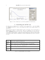
Currently, the priors for the independent factor effects and covariate coefficients are obtained
by the user entering values for the parameters that define them. Although this can also be
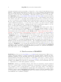
done for the exchangeable factor effects, a graphical feedback interface (GFI) is also provided
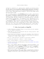
to facilitate this process. The GFI is shown in Figure 1. This figure shows the elicitation
option for an exchangeable factor’s prior in a Normal linear model. It is possible to consider
the effects’ standard deviation τ directly or, as shown, think in terms of the difference between
the effects of two randomly chosen levels of the factor. The user is asked to enter the maximum
credible size of this difference, this being interpreted as the approximate 95th percentile of its
prior distribution. Simulation work, not discussed here, has shown that if
τ
∼ Half-Normal(σ 2 )
δ ∼ Half-Normal(2τ 2 )
then
σ ≈ δ.95 /3
where δ.95 is the 95th percentile of the distribution of δ.
In BugsXLA the elicited maximum credible difference defined above is interpreted as 3σ.
The GFI is designed such that the graph of the prior distribution, as well as some of its
percentiles, is updated in real time as the user changes the credible difference using the
spinner control. It is possible to plot the exponential of the X-axis, this being useful when log
or logit link is used. When this transformation is applied the axis can then be interpreted as
the ratio (log) or odds-ratio (logit) of two randomly chosen effects.
8
BugsXLA: Bayes for the Common Man
Figure 1: Prior elicitation process via the graphical feedback interface.
5. Controlling the MCMC run
Probably the most difficult aspect to automate is the settings used to control the MCMC
run. BugsXLA allows direct control of the parameters in Table 2 (the default settings are in
parentheses).
It is not suggested that the default settings for these are adequate even for the majority of
GLMM’s that are likely to be fit in practice. Their use is primarily for the case when it is
unsure if WinBUGS will run the model at all, providing a quick and dirty run. They may also
be adequate for models with no exchangeable effects terms (“fixed” effects models). For this
reason the program offers three alternative pre-defined settings with some advice on when to
use them.
Burn In
(1000)
Samples
(1000)
Thin
(1)
Chains
(1)
Auto Quit
(Yes)
Number of initial MCMC samples to be discarded.
Convergence assumed past this point.
Number of MCMC samples to be generated from Posterior Distribution.
If set to K then only every Kth sample is saved. Use when high
autocorrelation is present to reduce the number of samples required to give
good coverage of the posterior distribution.
Number of separate chains to be generated.
Determines whether WinBUGS is automatically closed after the MCMC run.
Table 2: Default MCMC control settings.
Journal of Statistical Software
9
Simple model
(Burn In: 5,000 Samples: 10,000 Thin: 1 Chains: 1 Auto Quit: Yes)
Orthogonal design, may include one exchangeable effects term with variance estimate
having 3 or more effective degrees of freedom
Regular model
(Burn In: 25,000 Samples: 10,000 Thin: 10 Chains: 1 Auto Quit: Yes)
Nearly orthogonal design, may include covariate(s), but with each variance estimate
having 3 or more effective degrees of freedom. Although not part of the default settings,
I would recommend that ‘Auto Quit’ be turned off and at least 2 chains run so that
MCMC convergence can be checked before using the results.
Complex model
(Burn In: 100,000 Samples: 20,000 Thin: 50 Chains: 1 Auto Quit: No)
Messy design, may include covariate(s), or some variance estimates having less than
3 effective degrees of freedom. Note that ‘Auto Quit’ is turned off as it is strongly
recommended that MCMC convergence be checked before using the results. Although
not part of the default settings, I would recommend that at least 2 chains be run.
Mixing can often be greatly improved if informative priors are provided for poorly
estimated variance components. These need not be strong priors, just sufficiently precise
to effectively rule out incredibly large values.
Initial values are automatically generated using the following procedure:
• The lowest level precision parameter (Normal models) is initialised to 10 times the
precision of the response. This equates to an expected R2 of about 90%.
• Any independent factor effects are initialised to 0.3 times the minimum of the standard
deviation of the response and the prior standard deviation of the effect itself. The reason
for the 0.3 multiplier will be explained when multiple chains are discussed later.
• The standard deviation for exchangeable factor effects is initialised to 0.3 times the
minimum of the standard deviation of the response and the prior Half-Normal sigma
parameter for this term.
• The covariate regression coefficient is initialised to 0.3 times the minimum of the ratio
of standard deviations of the response and covariate, and the prior standard deviation
of this coefficient itself.
For both the independent factor effects and the covariate regression coefficients, the signs of
the initial values are alternated between successive terms fitted in the model. A maximum of 5
chains can be run using BugsXLA with the following multipliers for the default values defined
above used to obtain a range of initial values: 1, 0.1, 10, 0.3, and 3. These multipliers were
chosen so that initial values differing by one or two orders of magnitude would be obtained,
without getting values too far into the tails of the prior distribution.
Currently, I have only limited experience on which to comment on the adequacy of this advice.
I certainly would not unreservedly recommend this advice, and include it in the program
10
BugsXLA: Bayes for the Common Man
mainly as a placeholder for better guidance as experience with the program develops. I do
believe that providing such guidance is an essential feature of any software that is aimed at the
average data analyst. If nothing else, I would hope that this attempt would raise discussion
on the general guidance that can be given.
6. Worked example
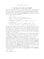
To illustrate how the user interacts with BugsXLA, the ‘Seeds’ example, originally from
Table 3 of Crowder (1978) but also used by Spiegelhalter, Thomas, Best, and Gilks (1996b),
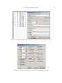
is reanalysed. Figure 2 shows the completed model specification form, in this case defining a
binomial error model with logistic link. The variables R and N contain the number germinated
and total number of seeds, respectively, in a study undertaken to assess the effects of seed
and root extract types. As well as fitting independent (“fixed”) main and interaction effects
for the “treatment structure”, over-dispersion is accommodated by including an exchangeable
(“random”) effects term for the 21 plates used in the experiment.
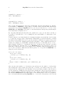
By clicking on the button labelled ‘MCMC & Output Options’ another form is shown that
allows the user to alter the default settings as given in Figure 3.
Importing ‘Stats’ or ‘Samples’ will result in the WinBUGS summary statistics or generated
samples from the posterior distribution being imported into Excel respectively. Selecting
‘Predicted Averages’ gives the predicted mean response for every possible combination of the
factors specified to have independent effects, averaged over the levels of any exchangeable
effects, and with any covariates set to their mean value. The scaled residuals are the raw
residuals divided by:
Normal error: σ
√
Poisson error: µ
Binomial error:
p
N µ(1 − µ)
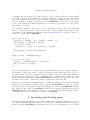
After setting these options and confirming that the model is specified correctly, the prior
distributions for each of the terms can be altered. Figure 4 shows the default settings for the
exchangeable effects of the plate term.
The button labelled ‘GFI’ would bring up the graphical feedback interface as illustrated in
Figure 1. In the ‘Seeds’ example, since a logit link has been specified, the user would be
prompted to think about his or her prior beliefs in terms of the odds-ratio of the effects of
two randomly chosen plates.
Once the user is satisfied with the priors, by clicking ‘OK’ the program generates all the files
needed by WinBUGS to complete the analysis: data files (including the constants needed to
define the model), initial value files, the code itself as well as the script file that controls the
WinBUGS analysis. Provided that a successful exit from WinBUGS is achieved, the user
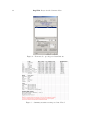
is then prompted to import the results, which in the case of the summary statistics will be
formatted as in Figure 5.
The column with the header ‘WinBUGS Name’ shows the generic node names used in WinBUGS and is of little use unless an experienced user wished to edit the code directly later.
Informative names for the parameters are given in the column with the header ‘Label’. Inspection of the summary statistics shows that the first level of each independent main effects
Journal of Statistical Software
Figure 2: Data in an Excel sheet, with the completed model specification form.
Figure 3: MCMC and output options form showing default settings.
11
12
BugsXLA: Bayes for the Common Man
Figure 4: Form used to specify prior distributions.
Figure 5: Summary statistics as imported into Excel.
Journal of Statistical Software
13
term has been constrained to zero, with appropriate constraints on the interaction effects
also. The output also provides a summary of the model fitted, plus the prior distributions
specified. It also records the settings for the MCMC run with the time taken to run. Due to
the inherent uncertainties currently associated with using MCMC sampling methods to tackle
generic problems, a final warning message is displayed to ensure the user remains cautious
when interpreting the results.
One of the distinct advantages of using WinBUGS is that it is possible to characterise the
whole posterior distribution by viewing and summarising the generated samples for any of
the parameters, or arbitrarily complex functions of them. This is particularly useful for
distributions that are distinctly non-Normal, such as the variance component for the plate
effect in this example. The imported samples can be subsequently pasted into your favourite
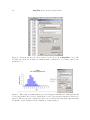
statistics package, and a histogram, or other summaries, created. Alternatively the ‘Post v
Prior’ icon on the BugsXLA toolbar can be selected, which runs a utility program that can
do this within Excel. Figure 6 shows the form that appears when this option is chosen.
After identifying the column of data to be graphed and clicking on ‘Update Parameter Information’ the name and prior specified for this parameter are shown. Clicking on update graph
will produce a plot of the posterior distribution (histogram) and prior overlaid. Figure 7
shows such a plot after adjusting the bins for the histogram using the options on the form.
7. Other functionality in BugsXLA
• Additional distributions and links: Weibull, t and log-Normal; probit and complementary log-log links for binomial data.
• Multinomial and ordered categorical data; the data can be either grouped into counts
or recorded as individual responses.
• Censored data: lower bound, upper bound, interval or any mixture of these. The button
labelled ‘Set Variable Types’ in Figure 2 launches a form that facilitates the classification
of variables as one of Factor, Variate or Censor.
• Factor by covariate interactions: easy fitting of group regression coefficients.
• Covariates with exchangeable coefficients, i.e., ‘random coefficients’.
• Allow over-relaxed samples to be generated as discussed in Neal (1998).
• Calculation and importing of the DIC statistic as defined in Spiegelhalter, Best, Carlin,
and van der Linde (2002).
• Able to create a ‘Bugfolio’ using the ‘Create Bugfolio’ feature shown in Figure 3. By
creating a Bugfolio all the files created by BugsXLA are stored in the folder specified.
This is useful for experienced WinBUGS programmers who wish to use BugsXLA to
generate some basic code and then modify the code, script or data files to run a more
complex model not possible using BugsXLA directly.
• Help is provided on-line by clicking on the ‘Help?!’ box found at the bottom left of
most of the forms (see Figure 2 for example). Features that have help text provided are
highlighted, and the help is obtained by moving the mouse over the highlighted area.
14
BugsXLA: Bayes for the Common Man
Figure 6: Form shown after the ‘Post v Prior’ icon is selected from BugsXLA toolbar. The
specified prior is shown, in this case a Half-Normal, constrained to be positive, with a scale
parameter of 5.
Figure 7: Histogram of 10,000 samples generated during the MCMC run. This graph should
closely approximate the posterior distribution for the between plates standard deviation parameter. The specified prior distribution has been overlaid (solid black line) suggesting that
the likelihood has dominated in the estimation of this parameter.
Journal of Statistical Software
15
8. Concluding remarks
The purpose of BugsXLA is to provide a tool that makes it easier for the average data analyst
to try Bayesian methods. By allowing models to be specified in a manner that is familiar to
users of such packages as SAS, S-PLUS and Genstat, it removes one of the major barriers to
those people who are curious but uncommitted to the Bayesian approach. An initial attempt
has been made to provide guidance on appropriate settings for the MCMC run when GLMMs
are being fitted. It is also shown how a prior elicitation interface could be integrated into a
Bayesian analysis program.
By removing the need to know how to code the models, import the data and export the
results, it allows the user to focus on the more important issues:
• Is the model appropriate?
• What priors can I justify?
• What inferences am I trying to make?
As well as providing a tool for tackling real problems, this could also provide a useful aid for
those teaching Bayesian methods.
As Spiegelhalter et al. (2003b) state in the BUGS manuals, “MCMC sampling can be dangerous!”. It could be argued that BugsXLA increases the risks due to the possibility of the
WinBUGS output being accepted without checking for convergence or satisfactory mixing.
These risks can be mitigated by education in how to use such software, as well as the software
providing appropriate guidance both during the specification of the model and MCMC run,
as well as during the analysis stage. BugsXLA offers some such guidance, but future packages
aimed at a broad audience need to offer much more. Ultimately, the most effective way to
grow the knowledge needed to feed this advice is to engage a much broader group of people
who regularly use GLMMs in business and industry. My hope is that BugsXLA can help to
encourage even more people to try Bayesian methods and, through its constructive criticism,
play a small part in the ultimate development of the first Bayesian software package truly
useable by the average data analyst.
References
Crowder MJ (1978). “Beta-binomial ANOVA for Proportions.” Applied Statistics, 27, 34–37.
Gelfand A, Smith AFM (1990). “Sampling-based Approaches to Calculating Marginal Densities.” Journal of the American Statistical Association, 85, 398–409.
Gelman A (2004). “Prior Distributions for Variance Parameters in Hierarchical Models.”
Report, Columbia University. URL http://www.stat.columbia.edu/~gelman/research/
unpublished/tau5.pdf.
Gilks WR, Roberts GO (1995). “Strategies for Improving MCMC.” In SR W R Gilks,
D Spiegelhalter (eds.), “Markov Chain Monte Carlo in Practice,” pp. 75–88. Chapman &
Hall, London.
16
BugsXLA: Bayes for the Common Man
Heiberger RM (1989). Computation for the Analysis of Designed Experiments. John Wiley
& Sons, Inc.
Lee PM (2004). Bayesian Statistics. An Introduction. Arnold, London, 3rd edition.
Neal R (1998). “Suppressing Random Walks in Markov Chain Monte Carlo using Ordered
Over-Relaxation.” In MI Jordan (ed.), “Learning in Graphical Models,” pp. 205–230. Luwer
Academic Publishers, Dordrecht.
Smith AFM, Roberts GO (1993). “Bayesian Computation via the Gibbs Sampler and Related
Markov Chain Monte Carlo Methods (with discussion).” Journal of the Royal Statistical
Society B, 55, 3–24.
Spiegelhalter D, Abrams K, Myles J (2003a). Bayesian Approaches to Clinical Trials and
Health-Care Evaluation. John Wiley & Sons Ltd.
Spiegelhalter D, Best N, Carlin B, van der Linde A (2002). “Bayesian Measures of Model
Complexity and Fit (with discussion).” Journal of the Royal Statistical Society B, 64,
583–640.
Spiegelhalter D, Thomas A, Best N, Gilks W (1996a). BUGS 0.5 Manual (version ii). MRC
Biostatistcs Unit, Cambridge, UK.
Spiegelhalter D, Thomas A, Best N, Gilks W (1996b). BUGS Examples Volume 1 (version
i). MRC Biostatistcs Unit, Cambridge, UK.
Spiegelhalter D, Thomas A, Best N, Lunn D (2003b). BUGS User Manual, Version 1.4. MRC
Biostatistcs Unit, Cambridge, UK.
Tierney L (1994). “Markov Chains for Exploring Posterior Distributions.” Annals of Statistics,
22, 1701–1762.
Journal of Statistical Software
17
A. Key elements of the WinBUGS language
I explain only enough here to enable anyone familiar with statistical modelling to follow the
code segments in the main paper. Most of this is directly copied from the BUGS 0.5 Manual
written by Spiegelhalter, Thomas, Best, and Gilks (1996a).
The code provides a declarative description of the probability model, which is compiled before
running. There are two types of relations:
~ which means “is distributed as”
<- which means “is to be replaced by”
These relations are used to define stochastic and deterministic nodes respectively. For example,
alpha
dnorm(mu, tau)
defines a Normally distributed variable, alpha, with mean mu and precision (1/variance) tau.
While,
mu <- beta*time
defines mu to be equal to the product of the two nodes beta and time; these latter nodes
could themselves either be variables or predefined constants.
Vectors and arrays are represented using square brackets, e.g., x[i, j]. The indexing convention broadly follows those of S-PLUS, so that, for example, x[, 3] indicates all the values
of the third column of the two dimensional array x.
Repetitive structures can be succinctly described using for loops. Note that these constitute
a declarative description of the model and should not be interpreted in a procedural way. The
syntax follows that of S-PLUS;
For (name in expression1 :expression2 ) { ... }
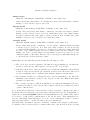
B. Downloading and installing BugsXLA
BugsXLA (v2.1) is a Microsoft Excel Add-In that is freely available via the BUGS website:
http://www.mrc-bsu.cam.ac.uk/bugs or direct from http://www.pipshome.freeserve.
co.uk/stats. After clicking on “Download BugsXLA (v2.1)” and saving the self-extracting
zip file to a convenient location on your PC, follow these instructions to install BugsXLA as
an Excel add-in. It is necessary to have Windows 98 or higher (tested on 98, 2000 and 2002),
MS Excel (tested on 2000 and 2002; will not work on 97), MS Notepad and WinBUGS v1.4
already loaded on your PC.
It is important that Excel be closed before starting.
1. Run the self-extracting zip file; by default this puts the files in
18
BugsXLA: Bayes for the Common Man
C:\Program Files\WinBugsXLA
2. Open MS Excel
3. Select Tools: Add-Ins and Browse in the directory to which the zipped files have been
extracted (see step 1), ensuring that Files of Type: All Files has been selected.
4. Select the file BugsXLA.sta and make sure that ‘BugsXLA’ has been checked in the
Add-Ins dialog box before clicking ‘OK’.
5. If you are warned that either WinBUGS or Notepad is not in ‘specified location’, click
‘Yes’ and alter the directory entries so that these programs can be found.
6. A toolbar titled ‘BugsXLA’ should appear that could be moved to your favoured location
on the Excel frame.
You can find an Excel Workbook with a few example data-sets in the ‘unzipped to’ directory
specified in step 1:
BugsXLA Egs.xls
Help is available on some of the BugsXLA forms. Click on the ‘Help?!’ checkbox and hover
the mouse over any areas that are highlighted.
Affiliation:
Phil Woodward
Biostatistics and Reporting
Pfizer Global Research and Development
Ramsgate Road, Sandwich
Kent, CT13 9NJ, United Kingdom
E-mail: [email protected]
Journal of Statistical Software
May 2005, Volume 14, Issue 5.
http://www.jstatsoft.org/
Submitted: 2004-06-23
Accepted: 2005-01-31