1
LuSci data processing.
User manual
A. Tokovinin, A. Berdja
Version 2. December 21, 2009
Contents
1 Installation
1
2 Data preparation (stage 1)
2.1 Processing overview . . . . . . . .
2.2 The input files . . . . . . . . . . .
2.3 The parameter file . . . . . . . . .
2.3.1 Site and data parameters .
2.3.2 Instrument parameters . . .
2.3.3 Data processing parameters
2.4 The WVP files . . . . . . . . . . .
.
.
.
.
.
.
.
2
2
2
3
3
4
4
5
3 From raw data to covariances (stage 2)
3.1 Data filtering and calculation of normalized covariances . . . . . . . . . . . . . . . . .
3.2 Power spectra from BIN files . . . . . . . . . . . . . . . . . . . . . . . . . . . . . . . .
5
5
7
4 Restoration of turbulence profiles
4.1 The weighting functions . . . . .
4.2 On the screen . . . . . . . . . . .
4.3 The TP output files . . . . . . .
4.4 Hard-coded parameters . . . . .
.
.
.
.
.
.
.
.
.
.
.
.
.
.
.
.
.
.
.
.
.
.
.
.
.
.
.
.
.
.
.
.
.
.
.
.
.
.
.
.
.
.
.
.
.
.
.
.
.
.
.
.
.
.
.
.
.
.
.
.
.
.
.
.
.
.
.
.
.
.
.
.
.
.
.
.
.
.
.
.
.
.
.
.
.
.
.
.
.
.
.
.
.
.
.
.
.
.
.
.
.
.
.
.
.
.
.
.
.
.
.
.
.
.
.
.
.
.
.
.
.
.
.
.
.
.
.
.
.
.
.
.
.
.
.
.
.
.
.
.
.
.
.
.
.
.
.
.
.
.
.
.
.
.
.
.
.
.
.
.
.
.
.
.
.
.
.
.
.
.
.
.
.
.
.
.
.
.
.
.
.
.
.
.
.
.
.
.
.
.
.
.
.
.
.
.
.
.
.
.
8
8
8
9
11
5 Use of the LuSci data products
5.1 IDL service . . . . . . . . . . . . . . . . . . . . . . . . . . . . . . . . . . . . . . . . . .
5.2 Plotting scripts . . . . . . . . . . . . . . . . . . . . . . . . . . . . . . . . . . . . . . . .
12
12
12
1
.
.
.
.
.
.
.
.
.
.
.
.
.
.
.
.
.
.
.
.
.
.
.
.
.
.
.
.
.
.
.
.
.
.
.
.
.
.
.
.
.
.
.
.
.
.
.
.
.
.
.
.
.
.
.
.
.
.
.
.
.
.
.
.
.
.
.
.
.
.
.
.
.
.
.
.
.
.
.
.
.
.
.
.
.
.
.
.
.
.
.
.
.
.
.
.
.
.
.
.
.
.
.
.
.
.
.
.
.
.
.
.
.
.
.
.
Installation
The actual package runs under the commercial language IDL. After downloading the compressed file,
unpack into a working directory.
The uncompressed directory should contain the following files:
1
• Readme.txt – short description
• IDL code for data processing:
go.pro – datproc7.pro – profrest4e.pro – lusci.common – profrest.common – service.pro.
• Astrometric programs from the ASTRO library:
ct2lst.pro – cirrange.pro – daycnv.pro – jdcnv.pro – moonpos.pro – mphase.pro – nutate.pro
– sunps.pro – ten.pro – posang.pro – isarray.pro – legend.pro – trim.pro.
• Matrix needed for lunar spectrum model: text files AA00 -- AA04 and the IDL file Mat400.idl
(the latter, if absent, will be created automatically).
• Test data and parameter file eso.par in tests/
• AWK plotting examples: plotcn2.awk* – plotcn2.par – plotsee.awk* – plotsee.par –
plotflux6.awk* – flux6.par.
• User guide code4.pdf (this file).
The code should be ready to use after unpacking.
Under the IDL prompt, in the working directory, type @go and see the results of processing the
data example in the tests/ directory. The go script has only two parameters in the text: name and
pfn:
- name: The file name without extension, usually lusci YYYY-MM-DD. where YYYY is the year, MM
the month and DD the day
- pfn: The parameter file, for example, tests/eso.par.
The plotting awk scripts require installation of the XMGRACE software.
2
Data preparation (stage 1)
2.1
Processing overview
Processing of LuSci data consists of 3 stages (Fig. 1):
1. Data preparation (this Section)
2. Calculation of covariances (Sec. 3)
3. Fitting turbulence profile (Sec. 4)
2.2
The input files
The input files, like in the tests/ directory, are usually:
• A DAT file, usually named lusci YYYY-MM-DD.dat, containing all the essential information for
data processing.
2
datadir
Parameter
file
.PAR
datproc7.pro
.DAT
.BIN
.COV
profrest4e.pro
.RES
matrices
.TP
service.pro
Figure 1: Data processing overview. The relevant parametes from the PAR file are used at stage 1 (covariance calculation with datproc7.pro) and stage 2 (turbulence profile fitting with profrest4e.pro).
The input data and results are in the datadir directory.
• A BIN file, usually named lusci YYYY-MM-DD.bin, that contains the raw flux measurements.
It cannot be used without the DAT file where the pointers are stored. This file can be used to
re-calculate covariances and to view the data (for quality control), but is usually not essential
for regular operation.
• A WVP file, usually named lusci YYYY-MM-DD.wvp, that contains 4 coefficients to calculate
ground wind speed as a function of time. If this file is present, the wind velocity is taken into
account for calculating the weighting functions. This issue will be developed in further versions
of this program.
2.3
The parameter file
The parameter file, for example eso.par, contains parameters needed for the data reduction (Table 1).
The syntax (brackets, commas) should be maintained carefully. Copy this file under a different name
and edit. Comments and commented lines are allowed.
2.3.1
Site and data parameters
The most important parameters are :
• long The site longitude in degrees, for Cerro Paranal -70.403 (note the sign).
• lat The site latitude in degrees, for Cerro Paranal -24.625 (note the sign).
• datadir The sub-directory containing data files (relative to the current directory or absolute
path). For example, if the package files are in a working directory ”/work” and the data files in
a sub-directory ”/work/tests”, then put ’tests/’. Do not forget the ending slash and comma!
3
Table 1: Use of parameters in the data processing
Parameter
long=... [deg]
lat=... [deg]
datadir=...
detdiam=0.01 [m]
detpos=[...] [m]
amplcoef=[...]
texp=0.002 [s]
basetime=5 [s]
accumtime=60 [s]
fhigh=250 [Hz]
flow=0 [Hz]
threshold1=0.05
threshold2=0.02
threshold3=0.02
threshold4=0.8
threshold5=1.
Zint=[...] [m]
2.3.2
datproc7.pro
no
no
data path
no
no
covariance calc.
power spectrum
yes
60-s binning
with /recomp
with /recomp
sky filtering
flux filtering
flux filtering
num. of points
variance uniform.
no
profrest4e.pro
astrometry
astrometry
data path
weighting func.
bases and WFs
no
wind filtering
no
no
no
no
no
no
no
no
no
integrals
Instrument parameters
Instrument parameters should be fixed for each scintillometer, they never change. The parameters file
eso.par is good for the ESO-Lusci standard instruments. The instrument parameters are:
• detdiam detector’s diameter in [m], actually 0.01 (1 cm).
• detpos detector’s positions in order of channels, with the position of channel 0 being zero. For
example, [0,0.19,0.23,0.25,0.28,0.40]. This also defines the number of detectors Ndet (6
for ESO arrays).
• amplcoef amplification coefficients for the AC signal component relative to DC component, in
each channel.
• texp exposure time in [s], actually 0.002 (2 ms).
2.3.3
Data processing parameters
• basetime is the time in [s] for each line of the DAT file, same as in the acquisition program. It
is used by the datproc7.pro to determine the number of lines to bin.
• accumtime is the time interval in [s] to average several lines for calculation of the covariances.
Usually it is set to 60 (1 min), but can be increased.
• fhigh is the upper cutoff frequency in Hz relevant for re-calculation of covariances from the BIN
files (paragraph 3.2). All signal above fhigh is rejected. Actually 250 (no filtering).
4
• flow is the lower cutoff frequency in Hz relevant for re-calculation of covariances from the BIN
files (paragraph 3.2). All signal below flow is rejected. Actually 0 (no filtering).
• Zint are user-defined heights in [m] to which the seeing integrals will be computed, actually [4.,
16., 64.,256.]. The user can change the values and number of these altitudes. However, an
easier way to calculate turbulence intergals to arbitrary heights is to use service.pro, without
re-processing the data.
The filtering parameters define the criteria to reject wrong data. The criteria are based on the
flux measurements in the DAT file [5].
• threshold1 is the maximum allowed fraction of SKY flux relative to the Moon flux, actually
0.05 or 5%.
• threshold2 is the maximum relative deviation of the flux in each channel from the 5-th order
polynomial fit of flux vs. time. All individual 5-s data points where at least in one channel the
difference is above threshold2 are rejected. Actually 0.02 or 2%.
• threshold3 is the maximum allowable change of the ratio of flux in each channel to the flux
in all channels from its average value. In other words, individual differences between channel
sensitivity must be stable to within threshold3, otherwise the 5-s data points are rejected.
Actually 0.02 or 2%.
• threshold4 is the minimum fraction of valid points within each accumtime, actually 0.8.
• threshold5 is the maximum relative difference of the variance in each channel relative to the
mean variance in all channels, actually 1.0. Points where strong fluctuations are found in some,
but not all, channels are rejected.
2.4
The WVP files
A wind velocity parameter’s WVP file is a ascii file sharing the same file name with the binary and data
files. It contains 4 numbers in one line, for example [0.052723 -1.321105 10.581735 -17.748143].
These numbers are w1 , w2 , w3 , w4 for instance. Wind velocity at the ground for a given UT-time (in
hours) U U T is calculated as v = w1 ∗ U U T 3 + w2 ∗ U U T 2 + w3 ∗ U U T + w4 . It is a representation of
the wind velocity during the measurements.
If the wind speed variations during the hours of observation with LuSci is known, it is possible to
create a WVP file by doing a cubic fitting to UT and storing the corresponding coefficients as shown
above.
3
3.1
From raw data to covariances (stage 2)
Data filtering and calculation of normalized covariances
The raw data consist of statistical moments of the signal (average values and raw covariances) stored
in the DAT file and of individual signal values (2-byte unsigned integers) stored in the BIN file.
5
The purpose of the 2-nd stage of the data processing is to calculate the variances and covariances
normalized by the flux. Sky and instrumental offset are taken into account. Wrong data are filtered
out according to the criteria in the parameter file. The result is written to a COV file (named
lusci YYYY-MM-DD.cov). The flux plot similar to one in Fig. 2 is saved in the data directory under
the name lusci YYYY-MM-DD flux.ps.
Figure 2: Flux plot vs. UT time (+24h) produced by datproc7.pro. The upper 6 curves show the
flux in ADU in 6 channels. The crossses in the middle at 1/2 of the flux level mark the rejected points.
The big squares at the bottom show sky measurements.
Normally, we will use the covariances from the DAT files. The IDL command will be
datproc, name, pf=pfn (see example in go.pro script).
If we want to re-compute the covariances from the BIN file (for checking or for frequency filtering),
the command is
datproc, name, pf=pfn, /recomp
In this case, the BIN file is needed and the filtering defined by the parameters fhigh and flow is
done. The result in the COV has the same format in both cases. The power spectrum averaged over
all channels and all valid measurements is displayed on the screen, the postscript plot is saved in a file
named like lusci YYYY-MM-DD pow.ps in the data directory. Note that the BIN file in the examples
is truncated (to save space), so the /recomp option will show an error.
For massive processing of DAT files there is a batch procedure
allproc, template, pf=pfn
where template can be something like lusci YYYY-MM or simply an empty string ’’ if all DAT files
are in the same directory anyway. The *.dat will be added to the template, then all files in the data
directory which match the template will be processed in one step. The option /recomp exists as well.
6
When using the allproc command, we do not check interactively the quality of each data file.
Each line of the COV file contains the following:
• Column 1: Name of the DAT file without extension
• Column 2: Julian day minus 2400000
• Columns 3 to 2 + Ndet : normalized variance in each channel, from 0 to Ndet − 1
• Columns 3 + Ndet to 2 + Ndet + Ndet ∗ (Ndet − 1)/2: normalized covariances. The order is as
follows: first, the covariances of channel 0 with channels 1,2,... Ndet − 1, then covariances of
channel 1 with channels 2,3, etc.
On the screen: The names of the compiled procedures appear on the screen. Then the name of
the parameter file is shown
Parameters from ---> tests/eso.par
When the processing of one file is finished, a summary appears:
234 time-averaged points
FILE_NAME
Time,h Navpts Npts Good Tot BadDC BadRel BadVar Sky Badsky
lusci_2009-11-26
4.89
234 2892 2580 2415
293
74
16
120
0
This summary (without header) is appended to the file datproc7.log, to keep track of the processed data. It shows the time period covered by the measurements in [h], the number of averaged
1-min. points, the total number of individual 5-s points (lines with M prefix in the DAT file). Then
follow the number of good data points which passed all quality criteria, the total number of points
used in the 60-s binning (some good points are left out because there are not enough in 1-min. chunk).
Finally, the last numbers show how many points were rejected by the ploynomial fitting (threshold2),
by the sensitivity criterion (threshold3), and by the variance uniformity (threshold5). The last two
numbers show the total number of sky measurements and the number of rejected sky measurements
(threshold1).
A plot of the fluxes vs. time appears after processing (Fig. 2). This is useful for visual evaluation
of the fraction of valid data and diagnostic of possible problem. Rejected points are makred by crosses
in this plot. By repeating the data processing with different filter settings, we can change the fraction
of accepted data.
3.2
Power spectra from BIN files
This sub-section can be skipped at first reading. The datproc7.pro contains two procedures which
are not used in normal data reduction, but are handy for checking the data quality. Temporal power
spectra can be calculated from the BIN files to verify the absence of pickup periodic noise, the signal
can be plotted as a function of time, etc.
Access to the BIN data is provided via pointers. These pointers and other relevant information is
stored in the binary IDL file named lusci YYYY-MM-DD.idl each time we run the allproc. So, run
this procedure before accessing the binary data! You do not need to use the recomp option. At the
7
same time, the parameter file is remembered in the common block, so the program “knows” where to
look for the data.
The binary data corresponding to the n-th accumtime period (normally one minute) are accessed
by the command
data = rd(name, n),
where name = ’lusci YYYY-MM-DD’ is the data file name without extension. If you don’t know
how many segments are in a given night, try n=0 first, the program reports the total number of “data
chunks” on the screen. Inconvenient, but workable. The structure data contains, among other things,
the array dat[X,Y,Z], where X = 6 is the number of detectors, Y = 2500 is the number of readings
in each basetime period (2500 = 5/0.002), and Z is the number of basetime periods in the given data
chunk (typically 10–12). The elements of this array are unsigned 2-byte integers read from the ADC
every 2 ms.
To plot the data in channel 3 as a function of time, use the command
plot, data.dat[3,*,*]
To see the temporal auto- and cross-covariance between channels 0 and 5, for example, type
cov, data, 0, 5
The screen displays first the temporal covariance, then (after pressing .C) the power spectra. Some
useful data are printed on the screen.
Finally, by typing relvar, data we obtain on the screen the relative variances in all channels.
This is useful for checking the amplification coefficients (all variances should be equal, on average).
4
Restoration of turbulence profiles (step 3)
The 3-rd stage of data processing fits a model of turbulence profile to the normalized covariances
prepared in the COV file. The model parameters are Cn2 values at 5 fixed distances from the instrument,
pivot points. The default pivot points are at 3, 12, 48, 192, and 768 m. Between these points, Cn2 (z) is
represented by power-law segments. The code profrest4e.pro takes COV files as input and produces
TP files with fitted parameters and other data as output. The same parameter file is used.
4.1
The weighting functions
The program is set to calculate the weighting functions which relate model with covariances every
hour. Computing the WFs takes some time, during which the screen shows a “progress bar” as
0%-10%-20%-40%-60%-60%-80%-Weights are computed!
After each WF calculation, the plot similar to Fig. 3 is displayed on the screen.
4.2
On the screen
Other than the compiled procedures, the information displayed on the screen during processing is as
follows:
• Parameters read from tests/eso.par. This reminds you the parameter file you are using.
• Reading wind-speed data from tests/lusci3 2009-04-11.wvp In the case when WVP file
exists, this message confirms that the wind velocity is taken into account in the WF calculation.
8
Figure 3: Weighting functions as displayed.
• Moon day ---------------------> 16.218488 The day (after new Moon) is displayed. This
parameter should be between 8 and 20 in order to have valid data reduction, otherwise the user
is advised to ignore the results.
• alpha = -->81.3865[deg] This is the anticlockwise angle of the Moon’s illuminated side relative to the instrument baseline.
•
0%-10%-20%-40%-60%-60%-80%-Weights are computed!
fore, while computing the weights.
The progress bar mentioned be-
While calculating the profile for every measurement, the Julian date, air mass, ground-layer seeing
[arcsec], and rms fit error are displayed:
54932.5908 1.558 0.406 0.031
54932.5916 1.549 0.331 0.034
54932.5931 1.534 0.288 0.025
The rms fit error is the rms difference between measured and fitted covariances divided by the
variance. At the end, the average fit error is displayed and the covariances are plotted (Figure 4).
4.3
The TP output files
The main output file is the TP file.
The TP file is a text file that has a header showing the following information:
• Covariance file name and location, for example # tests/lusci3 2009-04-11.cov
9
Figure 4: At the end of the processing, the average observed covariance (line) and the average theoretical covariance calculated from the reconstructed profiles (asterisks) are displayed.
• The profrest program version generating this TP file like # profrest4e.pro.
2009.
Dec.
21,
• pivot points, by default # Pivots 3.00 12.00 48.00 192.00 768.00.
• heights to which the seeing is integrated, # Zint 4.00 16.00 64.00 256.00, as entered in the
parameter file.
• Name of the parameter file used
• Contents of the parameter file in the form # Parameter-name parameter-value(s).
Then it displays the WVP parameters if a WVP file is provided, e.g. # Wind 0.0457790 -1.16856
9.53261 -15.6268.
Then follow the results, one line per accumtime period. Each data line contains:
• Column 1: Julian day minus 2400000
• Column 2: air mass
• Column 3: the seeing from the instrument up to the highest altitude in Zint in [arcsec].
• Column 4: the rms fit error of the covariance [1].
10
• Columns 5 to 4+ nz0 (number of pivot points, see paragraph 4.4): decimal logarithm of Cn2 in
[m−2/3 ] at pivot points [1].
• Columns 5+ nz0 to the end: optical turbulence integrals from the instrument (in fact starting
at 0.1 m distance) to the altitudes given by Zint, in [m1/3 ].
In addition to the TP files, the restoration program creates a RES file in the data directory
which lists the measured covariances in lines beginning with the prefix C and residuals (measured
− fitted)/variance in lines beginning with the prefix R. This file is provided for technical purposes,
for example to study any systematic deviations between measurements and model. A first-order
evaluation of such systematics can be done by the average covariance plot (Fig. 4).
4.4
Hard-coded parameters
Although most relevant parameters are gathered in the parameter file, some are fixed (hard-coded) in
profrest4e.pro. For the sake of completeness, we list these parameters here.
• Turbulence outer scale is fixed to 25 m. The user may choose another parameter at
L0 = 25.
; hard-coded outer scale, 25m
• The pivot points. Turbulence profile is fitted by power-law segments between the pivot points
located at fixed distance from the instrument (do not confuse with height). The default pivot
points are at 3, 12, 48, 192, and 768 m. The corresponding code segment in profrest4e.pro is
z0min = 3.
& nz0 = 5 & z0step = 4.
z0 = z0min*10^(findgen(nz0)*alog10(z0step))
The user may modify the first line, where z0min is the lowest pivot point, nz0 is the number of
pivot points, and z0step is the multiplicative step.
• The wind direction is fixed in profrest4e.pro, it is constant relative to the baseline. The
default value is π/4. The user can change it at this line:
windpar = [Texpo*wv, !pi/4] ; 45 deg to baseline
• The weighting functions are refreshed every hour. The user may choose to do this more often at
the following line in profrest4e.pro:
if (jdcurr-jdold gt 1./24.)
then begin
by changing 24 to a larger number.
• The data are processed only for air mass less than two. If you want to change this, modify the
following line:
if (am le 2.)
then begin ; ignore low Moon
11
5
5.1
Use of the LuSci data products
IDL service
A collection of IDL routines for working with TP files is provided in service.pro. It can be used “as
is” or, more likely, as a model for writing other applications.
The function gettp reads the data into IDL structure, for example
tp1 = gettp(’tests/lusci3 2009-04-13.tp’),
where the full name of the TP file is given as parameter. The structure
otp = {name:name,z0:z0,zint:zint,jd:jd,am:am,gsee:gsee,sig:sig,logcn2:logcn2,jturb:jturb}
contains the pivot points z0, the N -element arrays of Julian days, air mass, GL seeing, rms residuals,
etc., where N is the number of the data lines in the TP file. The array of y = log10 Cn2 has dimension
N × 5 for 5 pivot points, the array of turbulence integrals has dimension N × 4 if Zint has 4 elements.
This same function can be used to ingest data from several nights by using a template, e.g.
alltp = gettp(’tests/lusci3 2009-04*.tp’). This may be handy for some applications, but will
not work if we want to produce single-night plots.
The function profile(H, z0, y, airmass) returns a vector of Cn2 values for a number of heights
(not distances along the line of sight) specified in the input vector H. It takes account of the actual
heights of the pivot points (z0/airmass) and interpolates the fitted model to the given heights.
The next function turbint(Cn2, H, Hlim) returns the turbulence integral between Hlim = [Hmin,
Hmax], given the input profile and the height grid.
The procedure calcint, otp, Hlim uses the turbint function and the ingested structure to
calculate turbulence integral in the given height interval and to display it as a function of UT time.
The cn2plot, otp procedure displays a grey-scale plot of turbulence profile versus time, for a
given night. An alternative option to plot Cn2 (t) for a set of selected heights is offered by plottp.
Alternatively, plotsee.pro simply gives a graph of GL seeing vs. time.
The procedure avprof, otp takes the OTP structure (for a single night or for multiple nights)
to calculate average and median profiles. The plot also shows quartiles of the Cn2 (h) values at several
heights. The average OTP is fitted to a straight line in the log-log coordinates, log10 Cn2 (h) ≈ A +
B log10 h and the fit parametere A and B are displayed.
The procedure allint can process all .TP files matching a template and calculates the turbulence
integrals in the user-specified height limits. This procesure is not very useful in its present state, but
serves as an example for mass-processing the .TP files.
Using service.pro as a model, the user can develop his own tools for displaying or analysing the
turbulence profiles from LuSci.
5.2
Plotting scripts
As an alternative to IDL, we provide two simple scripts to plot the contents of TP files. These awk
scripts extract relevant data into temporary files, then call XMGRACE with suitable parameter files (also
provided in the package).
./plotcn2.awk tests/lusci3 2009-04-11.tp will produce a graph of Cn2 (t) at pivot points (not
at selected heights, as does the IDL program).
12
./plotsee.awk tests/lusci3 2009-04-11.tp will convert the turbulence integrals from the TP
file into seeing and plot them versus time. This plot gives an idea of the relative contribution of
different heights to the ground-layer seeing. The script makes attempt to determine the number of
pivot points by reading the preamble of the TP file, so it should work with more (or less) pivots, in
principle.
./plotflux6.awk tests/lusci3 2009-04-11.dat is a command to visualize the fluxes versus
time. This is a very useful tool for rapidly checking the data quality without IDL.
References
[1] A. Tokovinin, et al. ”Near-ground turbulence profiles from lunar scintillometer,” Mon. Not. R.
Astron. Soc. , in preparation, 2009
[2] A. Berdja, ”LuSci Matrix Moon Spectrum,” Internal report, CTIO, 2009
[3] A. Tokovinin, ”Restoration of continuous turbulence profile from lunar scintillation,” Internal
report, CTIO, 2008
[4] http://idlastro.gsfc.nasa.gov/ftp/
[5] A. Berdja, ”On Lusci data discrimination procedure,” Internal report, CTIO, 2009
13