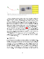
1
PARAMETRIC STRUCTURAL MODELING User Manual for Version 0.9.007 written by Clemens Preisinger contributions by Justin Diles and Robert Vierlinger September 7, 2011 Contents 1 Introduction 5 2 Disclaimer 5 3 Installation 5 4 Quick start 7 5 Usage 8 5.1 Dene the model geometry . . . . . . . . . . . . . . . . . . . 8 5.1.1 The LineToBeam-component . . . . . . . . . . . . . 8 5.1.2 The IndToBeam component . . . . . . . . . . . . . . 9 5.1.3 The ConToBeam-component . . . . . . . . . . . . . 10 5.2 The Assemble-component . . . . . . . . . . . . . . . . . . . . 10 5.3 The ModelView-component . . . . . . . . . . . . . . . . . . . 11 5.3.1 The Display Scales-submenu . . . . . . . . . . . . . 13 5.3.2 Display of cross section forces and moments . . . . . 14 5.3.3 Render settings . . . . . . . . . . . . . . . . . . . . . 14 5.4 Supports . . . . . . . . . . . . . . . . . . . . . . . . . . . . . . 15 5.5 Predened displacements . . . . . . . . . . . . . . . . . . . . 18 5.6 Loads . . . . . . . . . . . . . . . . . . . . . . . . . . . . . . . . 19 5.6.1 Point-loads . . . . . . . . . . . . . . . . . . . . . . . . 20 5.6.2 Mesh-loads . . . . . . . . . . . . . . . . . . . . . . . . 21 5.6.3 Gravity-loads . . . . . . . . . . . . . . . . . . . . . . 23 5.7 Analysis . . . . . . . . . . . . . . . . . . . . . . . . . . . . . . 23 5.8 Results . . . . . . . . . . . . . . . . . . . . . . . . . . . . . . 26 5.9 5.8.1 Section forces . . . . . . . . . . . . . . . . . . . . . . 26 5.8.2 Elastic energy . . . . . . . . . . . . . . . . . . . . . . 27 5.8.3 Nodal displacements . . . . . . . . . . . . . . . . . . How to change beam properties 28 . . . . . . . . . . . . . . . . 28 5.9.1 Bending stiness . . . . . . . . . . . . . . . . . . . . 28 5.9.2 Activation status of beams . . . . . . . . . . . . . . . 30 5.9.3 Height and wall-thickness of cross-sections . . . . . 30 5.9.4 Changing the default material . . . . . . . . . . . . . 30 5.10 Materials . . . . . . . . . . . . . . . . . . . . . . . . . . . . . . 31 5.10.1 Material properties denition . . . . . . . . . . . . . . 31 2 5.10.2 Material stiness . . . . . . . . . . . . . . . . . . . . . 31 5.10.3 Specic weight . . . . . . . . . . . . . . . . . . . . . . 32 5.11 Material selection . . . . . . . . . . . . . . . . . . . . . . . . 32 5.11.1 Theoretical background of stiness, stress and strain 33 5.12 Tips for designing statically feasible structures . . . . . . . . 34 5.13 Cross sections . . . . . . . . . . . . . . . . . . . . . . . . . . . 35 5.14 Cross section properties denition . . . . . . . . . . . . . . . 36 . . . . . . . . . . . . . . . . . . . 37 5.16 Evolutionary structural optimization . . . . . . . . . . . . . . 37 5.17 Bi-directional evolutionary structural optimization . . . . . . 39 . . . . . . . 41 . . . . . . . . . . . . . . . . . . . 42 5.19.1 Eigen-modes in structural dynamics . . . . . . . . . . 43 5.19.2 Eigen-modes in stability analysis . . . . . . . . . . . . 43 5.19.3 The EigenMode-component . . . . . . . . . . . . . . 43 5.20 Hints on reducing computation time . . . . . . . . . . . . . . 45 Utility Components 45 6.1 Nearest Neighbor . . . . . . . . . . . . . . . . . . . . . . . . . 45 6.2 Remove duplicate lines . . . . . . . . . . . . . . . . . . . . . . 45 6.3 Remove duplicate points . . . . . . . . . . . . . . . . . . . . . 45 6.4 Line-line-intersection . . . . . . . . . . . . . . . . . . . . . . . 46 5.15 The Dissemble-component 5.18 Elimination of tension or compression members 5.19 Eigen-modes of structures 6 7 8 Trouble shooting 46 7.1 Karamba does not work for unknown reason . . . . . . . . . 46 7.2 fem.karambaPINVOKE-exception . . . . . . . . . . . . . . 47 7.3 Karamba does not work after reinstalling Grasshoper . . . . 48 7.4 Predened displacements take no eect . . . . . . . . . . . . 48 7.5 The ModelView-component consistently displays all load cases simultaneously . . . . . . . . . . . . . . . . . . . . . . . . . . . 48 7.6 Icons in Karamba-toolbar do not show up . . . . . . . . . . 48 7.7 Error messages upon loading denitions saved with outdated Karamba versions . . . . . . . . . . . . . . . . . . . . . . . . . 48 7.8 Component in old denition reports a run-time error . . . . 48 7.9 Other problems . . . . . . . . . . . . . . . . . . . . . . . . . . 49 Version history 49 8.1 49 Version 0.9.06 - released on June 6, 2011 . . . . . . . . . . . 3 8.2 Version 0.9.007 - released on September 7, 2011 4 . . . . . . 49 1 Introduction Karamba is a Finite Element plug-in for the Rhino plug-in Grasshopper. It lets you interactively calculate the response of three dimensional beam structures under the action of external loads. Karamba is fully embedded in the parametric environment of Grasshopper. This makes it easy to combine parameterized geometric models, Karamba and optimization algorithms like Galapagos. 2 Disclaimer Although being tested thoroughly Karamba probably contains errors therefore no guarantee can be given that Karamba computes correct results. Use of Karamba is entirely at your own risk. Please read the licence agreement that comes with Karamba in case of further questions. 3 Installation These are the prerequisites for installing Karamba: Rhino 4.0 with Service Release 8 or 9 Grasshopper Build 0.8.0051. In case you do not possess Rhino 4 download a fully featured, free trial http://www.rhino3d.com/download.html. found at http://www.grasshopper3d.com/. version of from free can be Grasshopper which is Other versions of Grasshopper than that mentioned above may cause problems. We will try to keep up with Grasshoppers future development by providing corresponding Karamba versions. Check the download area of the Karamba web-site for corresponding information. Invoke KarambaSetup.msi and choose the folder where Grasshopper is installed when asked for an installation path. This is usually something like C://Programs/Rhinoceros 4.0/Plug-ins/Grasshopper. Besides other things a folder named Karamba will be created there, which contains the license agreement, a readme-le, pre-fabricated cross section and material 5 tables and the conguration le karamba.ini. The cong le can be edited with any text editor. It contains key - value pairs and is pretty self descriptive. If all goes well you will notice upon starting Grasshopper that there is a new category called Karamba on the component panel. It consists of eight subsections (see gure 1). In case you do not see any icons select Draw All Components in Grasshoppers View-menu. If you consistently get an fem.karambaPINVOKE exception see section 7.2 for how to solve that issue. Figure 1: Category ”Karamba” on the component panel These are the subsections which show up in the Karamba category: Algorithms: components for the calculation of statical models Cross Section: contains components to create and select cross sections for beams. Ensemble: lets you create models Loads: components for applying external forces Materials: components for the denition of material properties Params: classes of objects that make up the statical model Results: for the retrieval of calculation results Utils: contains some extra geometric functionality that is not directly linked to creating a model but makes certain things easy. ZZZ-Depricated: holds components which changed from an earlier version of Karamba to the current. They will be removed in some future version. In order to make denitions based on old versions work correctly they remain part of Karamba for the time being. 6 The colors of Karambas icons have a special meaning: black or white designates the entity or entities on which a component acts. Products of components get referenced by a blue symbol. This guide assumes that you have some basic knowledge of Rhino and Grasshopper. In case you need introductory material regarding Grasshopper it is probably a good idea to download the Grasshopper Primer from the Grasshopper web-site. 4 Quick start Creating a statical model in Karamba consists of six basic steps1 see g. 2: Figure 2: Basic example of a statical model in Karamba 1. Create wire-frame or point geometry for the structural model with Rhino or GH. 2. Convert 3. Dene wire-frame or point geometry to Karamba beams. which points are supports and which receive loads. Optional: Dene custom beam cross sections and multiple load cases. 4. Assemble the Karamba structural model with points, beams, supports and loads. 5. Analyze 6. View the Karamba structural model. the analyzed model. Deections can be scaled, stress, strain, etc. can be observed and multiple load cases can be viewed together or 1 This step-by-step procedure was devised and formulated by Justin Diles 7 separately. Mesh representations of beams can be rened to the desired resolution. Karamba is intended to provide an intuitive approach to statical modeling. All its components come with extensive help-tags and there are lots of examples on the web-site which can be easily customized according to ones own needs. So casual users can do without reading further. 5 Usage 5.1 Dene the model geometry First thing to do when setting up a statical model is to dene its geometry. In Rhino a given geometry consists of a collection of entities like points, lines and surfaces. For Karamba a given geometry consists of straight beams with physical properties (e.g. cross section, material). The next three subsections explain how to create them. 5.1.1 The LineToBeam-component Figure 3 shows how Karambas LineToBeam-component takes two lines as input, nds out how they connect and outputs beams as well as a set of unique points which are their end-points. Points count as identical if their common distance is less than that given in LDist the default value being 0.005[m]. The LineToBeam-component accepts only straight lines as ge- ometric input. Therefore polylines and the like need to be exploded into segments rst. Figure 3: The LineToBeam-component that turns two lines into beams All coordinates are in meter. In order to be of immediate use the beams come with a number of default values (see string-output in gure 3): active means that it will be included in the static model. Teh default cross section 8 is a circular prole of diameter 10[cm] with a wall-thickness of 0.33[cm]. The default material is steel of grade S235. The rst beam corresponds to the rst item in the list of input lines and so on. The order in which points appear in the output node-list is random by default. However it is sometimes advantageous to identify certain points by their list index in order to put loads on them or to dene supports. This can be achieved by feeding a list of coordinates into the Points-plug. They will be placed at the beginning of the output nodes-list. So in order that the end-points of the structure in gure 3 have index 0 and 1 it is necessary to input a list of points with coordinates (0/0/0) and (8/0/0). There are four more input plugs on the LineToBeam-component: New: If this plug has the value False only those lines will be added to the structure that start and end at one of the points given in the input points-list. Remove: If this option has the value True the LineToBeam-component checks for lines that lie on each other and merges such duplicates into one. This prevents an error that is hard to detect by visual inspection alone: Two lines on the same spot mean double member stiness in the statical model. LDist: sets the limit distance for two points to be merged into one. Lines of length less than that value will be discarded. Id: takes a list of strings as identiers for beams. If the number of items in this list is less than the number of beams then the last Id applies to the surplus beams. The default value is an empty string. Beams that meet at a common point are connected rigidly in the statical model like they were welded together. The Info output-plug informs about the number of removed nodes and beams. 5.1.2 The IndToBeam component Sometimes the initial geometry is already given as a set of points and two lists of node-indexes with one entry for each start- and end-point of beams respectively. In such a case it would be cumbersome to convert this information into geometric entities only for feeding it into the LineToBeam-component which reverses the previous step. The IndexToBeam-component (see gure 9 Figure 4: The IndexToBeam-component lets you directly define the connectivity information of beams 4) accepts a list of pairs of node-indexes and produces beams with default properties from it. This speeds up model generation considerably for there is no need to compare nodes for coincident coordinates. 5.1.3 The ConToBeam-component In Grasshopper meshing algorithms result in topological connectivity diagrams. With the help of the ConToBeam-component these may be directly converted to beam-structures (see gure 5). Figure 5: The ConToBeam-component turns connectivity diagrams into sets of beams 5.2 The Assemble-component In order to calculate the behavior of a real world structure one needs to dene its geometry, loads and supports. The component Assemble from the Ensemble subsection gathers all the necessary information and creates a statical model from it (see gure 6). In case that some beams were dened by node indexes then these will refer to the list of points given at the Pt input-plug. The output-plug Mass renders the mass of the structure in kilogram. When being plugged into a panel the model prints basic information about itself: number of nodes, beams, and so on. At the end of the list the characteristic length of the model is given which is calculated as the distance 10 Figure 6: The Assemble-component gathers data and creates a model from it. between opposing corners of its bounding box. 5.3 The ModelView-component The ModelView-component of the Ensemble subsection can be used to check the current state of a statical model (see gure 6). When adding a ModelView to the denition it is a good idea to turn o the preview of all other components so that they do not interfere. Clicking on the black menu headings unfolds the ModelView and unveils additional widgets for tuning the model display. Each of these will be explained further below. The range and current value of the sliders may be set by double-clicking on the knob. Figure 7: Partial view of a model. The ModelView-component features ve plugs on its left side: Model expects the model to be displayed LC-Factor can be used to scale individual load cases (see further 11 below). LC-Index lets one select the visible load-case (see example 'EModesWall.ghx'). The value in LC-Index will be added to the load-case selected in the drop-down-list of ModelView. If the resulting number is larger than the number of available load-cases the ModelView turns red. If the resulting value is smaller than 0 all load-cases are superimposed. The possibility of using a number-slider for selecting load-cases makes life easier in case that there are many of them. Colors: Color plots for stresses, strains etc. from blue to white to red by default. use a color spectrum One can customize the color range by handing over a list of RGB-values to the Colors-plug. There have to be at least three colors given. The rst color is used for values below, the last color for values above the current number range. The remaining colors get evenly distributed over the number range. The Grasshopper component Gradient can be used to generate the list of colors (see g. 8). Id: This plug lets one select those parts of a model which shall be displayed. It expects a list of strings. The default value is an empty string which means that all of the model shall be visible. As one can see in g. 7 it is possible to input regular expressions. These must start with the character & and adhere to the conventions of regular expressions as dened for C#. The identier of each beam of the model is compared to each item of the given string list. In case a list entry matches the beam identier the beam will be displayed. Fig. 7 contains four examples of Id lists: The rst would limit visibility to beam A, the second to beam B. The third is a regular expression which matches beams A or C. The fourth matches beams A to C. There are ve output plugs on the ModelView-component: Model is essentially the model which was fed in on the left side. When there are results available from a statical calculation deections are scaled and added to the node coordinates so that it contains the deformed geometry. From the Mesh output-plug you can get the mesh of the rendered model for further processing. In fact it is a list of meshes with each 12 Figure 8: Color plot of strains with custom color range. item corresponding to one element. The Curve plug delivers the axes of the deformed structure as interpolated 3rd degree nurb-splines. Use the Length/Subdivision slider to set the number of interpolation points. Legend C and Legend T provide lists of colors and strings which can be fed into Grasshoppers Legend-component (see g. 8). The numbers on the right side of the Legend correspond to the lower limit that the corresponding color represents. The number of color shades can be set in the karamba.ini le. 5.3.1 The Display Scales-submenu Figure 9: Local axes of cantilever composed of two beam elements. The Display Scales-submenu contains check boxes and sliders to enable/disable and scale displacements, load-symbols, support-symbols and 13 local coordinate systems. The displacement scale inuences the display and the output at the model-plug. It has no eect on stresses, strains, etc.. The colors of the local coordinate axes red, green, blue symbolize the local X-, Y-, and Z-axis. 5.3.2 Display of cross section forces and moments Figure 10: Moment My (green) about the local beam Y-Axis and shear force Vz (blue) in local Z-direction. The section forces sub-menu lets you plot section forces and moments as curves, meshes and with or without values attached. All generated curves and meshes get appended to the ModelViews curve and Mesh output. The graphical representation is oriented according to the local coordinate axes of the beam and takes the un-deected geometry as its base. The index of bending moments indicates the local axis about which they rotate, for shear forces it is the direction in which they act (see also g. 21). Customize the mesh-colors vie karamba.ini. The slider Length/Subdivision in sub-menu Render Settings controls the number of interpolation points. 5.3.3 Render settings The Render Settings menu contains checkboxes for displaying dierent aspects of a model: When activated Cross section, Strain, Stress and Utilization result in a rendered view of the model. Utilization is the ratio between the stress at a point and the yield stress of the corresponding material. Shear is neglected for calculating strains, stresses and utilization. Do not be disappointed that the colors do not change when switching from 14 strain to stress to utilization. The color range starts at the minimum value and stretches to the maximum. In case the model consists of one material, the zone of highest strain will also be the zone of highest stress and material utilization. Use a legend-component (see below) to get additional information out of color plots. Node tags attaches node-indexes to each node when active Element ids displays the beam identiers CroSec names shows the cross-section name used for each beam 5.4 Supports Without supports a structure would have the potential to freely move around in space. This is not desirable in case of most buildings. The current version of Karamba does statical calculations. This means that there must always be enough supports so that the structure to be calculated can not move without deforming. Thus rigid body modes are prohibited. When dening the supports for a structure one has to bear in mind, that in three dimensional space a body has six degrees of freedom (DOFs): three translations and three rotations (see gure 11). The structure must be supported in such a way that none of these is possible without invoking a reaction force at one of the supports. Otherwise Karamba will refuse to calculate the deected state. Sometimes you get results from moveable structures although you should not: The reason for this lies in the limited accuracy of computer-calculations which leads to round-o errors. Sometimes one is tempted to think that if there act no forces in one direction consider e.g. a plane truss then there is no need for corresponding supports. That is wrong: What counts is the possibility of a displacement. Bad choices of support conditions constitute a source of errors that is hard to track. Later on it will be shown how to calculate the eigen-modes of a structure. This kind of calculation works also in cases of moveable structures: rigid body modes if present correspond to the rst few eigen-modes. Figure 12 shows the geometry developed above with supports added at the endpoints of the structure. The Karamba/Ensemble/Support-component takes as input either the index3 or the coordinates of the point (or a list 3 In order to nd out the index of a specic node enable the tag-checkbox in the ModelView- component. See section 5.1.1 on how to predene the index of specic nodes 15 Figure 11: Metaphor for the six degrees of freedom of a body in three-dimensional space. Figure 12: Define the position of supports by node-index or position. with indexes or positions of points) to which it applies. Six small circles on the component indicate the type of xation: The rst three correspond to translations in global x, y and z-direction, the last three boxes stand for rotations about the global x,y and z-axis. Filled circles indicate xation which means that the corresponding degree of freedom is zero. The state of each box can be changed by clicking on it. The string output of the component lists node-index or nodal coordinate, an array of six binaries corresponding to its six degrees of freedoms and the number of load-case to which it applies. Supports apply to all load cases by default. From the support-conditions in gure 12 one can see that the structure is a simply supported beam: green arrows symbolize locked displacements in the corresponding direction. The translational movements of the left node 16 (a) (b) Figure 13: Influence of support conditions – undeflected and deflected geometry. Left:All translations fixed at supports. Right: One support moveable in horizontal direction. are completely xed. At the right side two supports in y- and z-direction suce to block translational movements of the beam as well as rotations about the global y- and z-axis. The only degree of freedom left is rotation of the beam about its longitudinal axis. Therefore it has to be blocked at one of the nodes. In this case it is the left node where a purple circle indicates the rotational support. The displacement boundary conditions may inuence the structural response signicantly. Figure 13 shows an example for this: when calculating e.g. the deection of a chair, support its legs in such a way that no excessive constraints exist in horizontal direction otherwise you underestimate its deformation. The more supports you apply the stier the structure and the smaller the deection under given loads. Try changing support conditions in PortalFrame.ghx in the examples on the karamba web-site and observe how the maximum deection changes. In order to arrive at realistic results introduce supports only when they reliably exist. By default the size of the support symbols is set to approximately 1.5[m]. The slider with the heading Support on the ModelView-component lets you scale the size of the support symbols. Double click on the knob of the slider in order to set the range of values. 17 5.5 Predened displacements Supports as described above are a special case of displacement4 boundary condition: They set the corresponding degree of freedom of a node to zero. The more general PreDisp-component lets you preset arbitrary displacements at nodes. Figure 14 shows a beam with prescribed, clockwise rotations at both end-points. See also example FixedFixedBeam.ghx. The PreDisp-component resembles the Support-component to a large degree: Nodes where displacement conditions apply can be selected via nodeindex5 or nodal coordinates. The size of the list fed into the Pos|Ind-plug determines the number of displacement conditions. All other input will be truncated or blown up by copying its last list item. Input-plug LCase lets you set the index of the load-case in which displacements shall have a specied value. The default value is -1 which means that the displacement condition is in place for all load-cases. It is not possible to have displacement boundary active in one load-case and completely disabled in others: For load-cases not mentioned in LCase the PreDispcomponent will act like a simple support with xed degrees of freedom equal to zero. Figure 14: Left: Deflection of a beam under predefined displacements at its end-supports; Right: PreDisp-component for setting displacement condition at left support. The Trans- and Rot-input-plugs expect vectors. They dene nodal translations and rotations in global coordinates. Translations are to be given in meter, rotations in degree. The X-component of the rotation vector describes a rotation about the global X-axis. A positive value means that the node rotates counter-clockwise if the X-Axis points towards you. Analog denitions apply to rotations about the global Y- and Z-axis. Karamba is based on the assumption of small deections. Thus be aware that large 4 The term displacement as used throughout this manual includes translations and rota- tions. 5 In order to nd out the index of a specic node enable the tag-checkbox in the ModelViewcomponent. See section 5.1.1 on how to predene the index of specic nodes 18 prescribed displacements and rotations give rise to incorrect results (which can nevertheless be used for shape-nding). In order to approximate eects due to large displacements apply them in several steps (e.g. see example FixedFixedBeam.ghx). Displacements can only be prescribed if the corresponding displacement degree of freedom is removed from the statical system. This means you have to click on the corresponding button in the Conditions-section of the PreDisp-component. The rst three buttons stand for translations the last three for rotations. Only those components of the Trans- and Rot-vectors take eect which correspond to activated conditions. 5.6 Loads Currently Karamba supports three kinds of loads: point-, mesh- and gravityloads. An arbitrary number of point- or mesh-loads and one gravity-load may be combined to form a load-case of which again an arbitrary number may exist. Figure 15 shows the denition of loads with the help of Gravity- and Point-load components. On the bottom of the ModelView-component there is a drop-down-list (unfold it by clicking on the Load-case Selection-menu header) which can be used to select single load-cases for display. Select all in order to view all existing load-denitions of all load-cases simultaneously. Use the force-slider to scale to size of the load-symbols (double-clicking on its knob lets you change the value range and its current value). Figure 15: Simply supported beam with three loads and three load-cases. 19 5.6.1 Point-loads The component Karamba/Ensemble/Point-Load lets you dene point loads. These get attached to points either by node-index6 or node-position. Feed a corresponding list of items into the Pos|Ind-plug (quite analogous to the Support-component). A point-load is given as a vector. Its components dene the force-components in global x-, y- and z-direction. The number of point-loads generated follows from the longest list principle 7 applied to all input. The output of the force-component has to be connected to the corresponding plug of the assembly. Plugging a point-load into a panel component gives the following information: Node-index where the load gets applied, force-vector and number of the load case to which it belongs. Karamba expects all force-denitions to be in kilo Newton(kN). On earth the mass of 100kg corresponds to a weight force of roughly 1kN . The exact number would be 0.981kN but 1kN is normally accurate enough. contains the specic weight of some everyday materials. Table 1 Rules of thumb numbers for loads can be found in table 2. Do not take these values too literally. For example the snow load varies strongly depending on the geographical situation. Loads acting along lines or on a specied area can be approximated by point-loads. All you need to do is estimate the area or length of inuence for each node and multiply it with the given load value. The Mesh-load- component (see next section) automates this task for surface loads. type of material [kN/m3 ] reinforced concrete 25.0 glass 25.0 steel 78.5 aluminum 27.0 r wood 3.2 snow loose 1.2 snow wet 9.0 water 10.0 Table 1: Specific weights of some building materials 6 In order to nd out the index of a specic node enable the tag-checkbox in the ModelView- component. See section 5.1.1 on how to predene the index of specic nodes 7 Longest list principle means that if the input consists of lists of dierent length, then the longest one determines the length of all the others: They get blown up by adding their last element for as many times as required. 20 loads [kN/m2 ] type life load in dwellings 3.0 life load in oces 4.0 snow on horizontal plane 1.0 cars on parking lot (no trucks) 2.5 trucks on bridge 16.7 Table 2: Loads for typical scenarios By default point loads will be put into load case zero. Any positive number fed into the LCase-plug denes the load case to which the corresponding load will be attributed. A value of −1 signals that the load acts in all existing load cases. 5.6.2 Mesh-loads The Mesh-load-component can be used to transform surface loads into equivalent nodal loads. This lets you dene life-loads on oor slabs, moving loads on bridges (see example Bridge.ghx in the examples collection on the Karamba web-site), snow on roofs, wind-pressure on a facade, etc... Figure 16 left side shows a simply supported beam and a mesh which consists of two rectangular faces. Each face covers one half of the beam span. The orange arrows symbolize the equivalent nodal forces. One can see that the equivalent force in the middle of the beam is twice as large as those at the supports. The procedure for calculating nodal forces from surface loads consists of the following steps: First Karamba calculates the resultant load on each face of the given mesh. Then the resultant loads of each face get evenly distributed among their corresponding vertices. The second step consists of distributing the vertex-loads among the nodes of the structure: this is done by considering the distance between the vertices and structure-nodes where the mesh load shall apply. Each vertex transfers its load to the nearest such node. In case that there are several nodes at equal distance the vertex load gets evenly distributed among them. Dierences of distance of less than 5mm are neglected. From the algorithm described above one can see that a crude mesh may lead to a locally incorrect distribution of loads. The right side of gure 16 shows what data the Mesh-load-component 21 Figure 16: Simply supported beam loaded with three forces that approximate an evenly distributed surface load on a mesh. collects: The input-plug Vec expects a vector or list of vectors that dene the surface load. Its physical units are kilo Newton per square meter (kN/m2 ). The orientation of the load-vector depends on the checkbox selected under Orientation (see also gure 17): local to mesh: X-component of the force vector is at right angle to the mesh-face; the Y-component acts horizontally if the mesh-face Xaxis is not parallel to the global Z-axis. Otherwise the Y-component of the force is parallel to the global Y-axis. This means a surface load with components only in X-direction acts like wind pressure. global: The force-vector is oriented according to the global coordinate system. This makes the surface load behave like additional weight on the mesh plane. global proj.: The force-vector is oriented according to the global coordinate system. The corresponding surface load is distributed on the area that results from projecting the mesh-faces to global coordinate planes. In such a way the action of snow load can be simulated. Figure 17: Orientation of loads on mesh: (a) local; (b) global; (c) global projected to global plane. 22 The input-plug Mesh accepts the mesh where the surface load shall be applied. Its vertices need not correspond to structure nodes. The mesh may have any shape. In order to dene the structure nodes where equivalent point-loads may be generated plug a list of their coordinates into the Pos-plug. These need to correspond with existing nodes otherwise the Assembly-component turns red. Oending nodes will be listed in its run-time error message. Set the LCase-input to the index of the load case in which the surface load shall act. Indexing of load-cases starts with zero, -1 is short for all load cases. For input plugs Vec, Mesh and LCase the longest list principle applies. 5.6.3 Gravity-loads Each load case may contain zero or one denition for the vector of gravity. In this way one can e.g. simulate the eect of an earthquake by applying a certain amount of gravity in horizontal direction. For Vienna which has medium earthquake loads this amounts to approximately 14% of gravity that a building has to sustain in horizontal direction. In areas with severe earthquake loads this can rise to 100%. The gravity component applies to all active beams in the statical model. The gravity vector denes the direction in which gravity shall act. A vector of length one corresponds to gravity as encountered on earth. 5.7 Analysis With geometry, supports and loads dened the statical model is ready for further processing. The Analysis-component computes the deection for each load case and adds this information to the model. Whenever the Analysiscomponent reports an error (turns red) despite the fact that the Assemble component works, it is probably a good idea to check the support conditions. Figure 18 shows a deected beam. The analysis component not only computes the model deections but also outputs the maximum nodal displacement (in meter),the maximum total force of gravity (in kilo Newton) and the structures internal deformation energy from each load case - see section 5.8.2 for details on work and energy. These values can be used to rank structures in the course of a structural optimization procedure: the more ecient a structure the smaller the max- 23 Figure 18: Deflection of simply supported beam under single load in mid-span. imum deection, the amount of material used and the value of the internal elastic energy. Real structures are designed in such a way that their de- ection does not impair their usability. See section 5.12 for further details. Maximum deection and elastic energy both provide a benchmark for structural stiness yet from dierent points of view: the value of elastic energy allows to judge a structure as a whole; The maximum displacement returns a local peak value. When activating the preview property of the Analysis-component the undeected structure shows up. In order to view the deected model use the ModelView-component and select the desired load case in the menu Load case Selection. There exist two options for scaling the deection output. First there is a slider entitled Deformation in the menu Display Scales that lets you do quick ne-tuning on the visual output. Second option: the input-plug LC-Factor which accepts a list of numbers that ModelView uses to scale the loads. Its default value is 1.0. Each item in the list applies to a load case. If the number of items in this list and the number of load cases do not match then the last number item is copied until there is a one to one correspondence. The second option for scaling displacements can be used in the course of form-nding operations: The model-plug at the right side of the ModelView outputs the displaced geometry which can be used for further processing. Selecting item all on the drop-down-list for the selected load case results in a superposition of all load cases with their corresponding scaling factor. Looking at gure 18 one immediately notices that only beam center axes are shown. In order to see the beams in a rendered view activate the Cross section-checkbox on the ModelView-component in Menu. This results in an image such as in gure 19(a). The mesh of the rendered image is available 24 (a) (b) Figure 19: Rendered images of the beam. Left: Only deflections enabled. Right: Deflections and strains enabled. at the Mesh-output of the model view. Two sliders control the mesh-size of the rendered beams: First Length/Subdivision determines the size of sections along the middle axis of the beams. Second Faces/Cross section controls the number of faces per cross-section. Figure 20: Mesh of beams under dead weight with Render Color Margin set to 5%. It is instructive to see which parts of a beam are under tension or compression. Activate the Strain-checkbox in menu Render Settings in order to display the strains in longitudinal beam direction. Red (like brick) means compression, blue (like steel) tension. Strain is the quotient between the increase of length when loaded and the initial length of a piece of material (compressive strain is negative, tensile strain positive). In some models there may exist small regions with high strains with the rest of the structure having comparatively low strain levels. This results in a strain rendering that is predominantly white and not very informative. With the slider Render Color Margin of the Render Settings Menu you can set the percentage 25 of maximum tensile and compressive strain at which the color-scale starts. Compressive strain values beyond that level appear yellow, excessive tensile strains pink (see gure 20). 5.8 Results 5.8.1 Section forces The S-Force component retrieves axial forces N and resultant bending moments M for all elements and load cases. See g. 21 for the denition of N and M. The order of element results corresponds to the order of beams. Thus the data can be used for cross section design. Figure 21: Normal force N and resultant moment M at cross section with local coordinate axes XYZ. Figure 22 shows a simply supported beam with two load cases presented in one picture. The beam consists of two elements and has a total length of eight meters. In load case zero a vertical force of magnitude 1kN acts vertically downwards in the middle of the beam. Load case one consists of a point-load of 3kN directed parallel to the un-deformed beam axis. The results at the output-plugs N and M in g. 22 are a three-dimensional trees that hold the beams Normal force in kilo Newton [kN] and resultant bending Moment in kilo Newton times meter [kNm] respectively. There is only one model fed into the S-Force component thus the rst index is zero. The second index refers to the load case: the rst two lists contain results for load case zero, the last two for load case one. Index three corresponds to the element indices in the model. Tensile normal forces come out positive, compressive normal forces have negative sign. The resultant moment yields always positive values as it is the length of the resultant moment vector in the plane of the cross section. 26 Figure 22: Simply supported beam under axial and transversal point-load: List of Normal forces and moments for all elements and all load cases. Karamba currently computes section forces at the endpoints of elements and returns their maximum values. In case of zero gravity the maximum values of M and N occur at the endpoints. With gravity switched on these maxima may lie inside the elements. In order to get a good approximation of the maximum cross section forces divide the elements in little pieces. As M is always rendered positive the maximum at the end points is unambiguously given. Under gravity normal forces in a beam may change sign. In such a case Karamba returns that N which gives the maximum absolute value. Let us take a look at the output in g. 22. In load case zero both elements return zero normal force because there acts no external axial load. The maximum moment of both elements is 2[kN m]. For a simply supported beam under a mid-point transverse load the maximum moment occurs in the middle and turns out to be M = F · L/4 = 1[kN ] · 8[m]/4 = 2[kN m]. The axial force of 3[kN ] in load case one ows to equal parts into both axial supports. It causes tension (1.5[kN ]) in the left element and compression (−1.5[kN ]) in the right one. 5.8.2 Elastic energy In mechanics energy is equal to force times displacement parallel to its direction. Think of a rubber band: if you stretch it you do work on it. This work gets stored inside the rubber and can be transformed into other kinds of energy. You may for example launch a small toy airplane with it: then the elastic energy in the rubber gets transformed into kinetic energy. When stretching an elastic material the force to be applied at the beginning is zero and then grows proportionally to the stiness and the increase of length of the material. The mechanical work is equal to the area beneath the 27 curve that results from drawing the magnitude of the applied force over its corresponding displacement. In case of linear elastic materials this gives a rectangular triangle with the nal displacement forming on leg and the nal force being its other leg. From this one can see, that for equal nal forces the elastic energy stored in a material decreases with decreasing displacements which corresponds to increasing stiness. The structure of the results list returned from the E-Energy component resembles that of the S-Force component described above. Instead of normal force and moment the work of normal force and moment on each beam are given. 5.8.3 Nodal displacements The Disp component lists the displacements of each node for all load cases. Again two trees with three dimensions form its output. These dimensions correspond to Model/LoadCase/Node. The data for each node at the output plugs Trans and Rot consists of three values each: three translations and three rotations. All of them are given in the global coordinate system in meter and radiant. A positive rotation say about the global X-axis means that the node rotates counter clockwise for someone who looks at the origin of the coordinate system and the X-axis points towards him or her. 5.9 How to change beam properties By default Karamba assumes the cross-section of beams to be steel tubes with a diameter of 10[cm] and a wall-thickness of 0.33[cm]. When two beams meet they are rigidly connected like they were welded together. Use the ModifyBeam-component to set the beam properties according to your choice. Figure 23 shows how this can be done by inserting it in front of the Assemble-component. By default the ModifyBeam-component leaves all incoming beams unchanged. Negative values for input properties take no eect. The size of the lists of input data is scaled to match the number of input beams by copying their last item. Several ModifyBeam-components may act consecutively on the same beam. 5.9.1 Bending stiness Beams resist normal force and bending. Setting the Bending-plug of the ModifyBeam-component to false disables bending stiness and turns the 28 Figure 23: Modification of the default beam properties. corresponding beam into a truss. There exist reasons that motivate such a step: Connections between beams that reliably transfer bending and normal force are commonly more expensive than those that carry normal force only. The design of connections heavily depends on the kind of material used: rigid bending connections in wood are harder to achieve than in steel. Yet rigid connections add stiness to a structure and reduce its deection. Therefore you are always on the safe side if you use truss elements instead of beams. For beams with small diameter compared to their length the eect of bending stiness is negligible compared to axial stiness. Just think of a thin wire that is easy to bend but hard to tear by pulling. Abandoning bending stiness reduces computation time by more than half for each node with only trusses attached. Karamba bases deection calculations on the initial, undeformed geometry. Some structures like ropes are form-active. This means that when a rope spans between to points the deformed geometry together with the axial forces in the rope provide for equilibrium. This eect is not taken into account in Karamba. In Karamba only the bending stiness of the rope (which is very small) keeps it from deecting indenitely. One way to circumvent this lies in using a truss instead of a beamelement. The second possibility would be to reduce the specic weight of the rope to zero (see further below). The third possibility would be to start from a slightly deformed rope geometry and apply the external loads in small steps where the initial geometry of each step results from the deformed geometry of the previous one. 29 Trusses only take axial forces. Therefore they do not prevent the nodes they are connected to from rotating. In case that only trusses attach to a node, Karamba automatically removes its rotational degrees of freedom. Otherwise the node could freely rotate which is a problem in static calculations. As soon as one beam connects to a node the node has rotational degrees of freedom. Bear this in mind when the Analysis-component turns red and reports a kinematic system. Transferring only axial forces means that a truss reduces a nodes movability in one direction. A node that is not attached to a support has three translational degrees of freedom. Thus there must be three truss elements that do not lie in one plane for a node to be xed in space. 5.9.2 Activation status of beams When set to true this option excludes the corresponding beam from further calculations until it is reset to true. 5.9.3 Height and wall-thickness of cross-sections Height which in case of circular tubes is equivalent to the outer diameter D and wall-thickness of a cross-section determine a beams axial and bending stiness. Karamba expects both input values to be given in centimeter. The cross-section area is linear in both diameter and thickness whereas the moment of inertia grows linearly with thickness and depends on D 3 . So in case of insucient bending stiness it is much more eective to increase a beams height (or diameter) than increasing its wall thickness. If a cross- section hight D is given but no wall thickness t then Karamba assumes t = D/30 by default. 5.9.4 Changing the default material Steel is the default material of all elements. The default grade is S235 which means that it yields at fy = 23.5[kN/m2 ].The next section shows how to dene materials with arbitrary properties or how to select predened materials from a data base. Feed these into the Mat input-plug of the ModifyBeam- component in order to override the default values. 30 5.10 Materials There are two ways for dening a material in Karamba: Either select a material by type from a data-base (see section 5.11) or set each material property manually (see below). 5.10.1 Material properties denition The component MatProps lets one directly dene material properties (see g. 24). These are Young's Modulus E Shear modulus G specic weight gamma yield stress fy Figure 24: The definition of the properties of two materials via the MatProps component. In addition to these, user dened materials can be given a name via the input-plug Name for identication in later stages of calculation. 5.10.2 Material stiness The stiness i.e. resistance of a material against deformation is characterized by its Young's Modulus or modulus of elasticity E . the stier the material. The higher its value Table 3 lists E -values for some popular building materials. For composite materials like in the case of rods made from glass ber and epoxy it is necessary to defer a mean value for E by material tests. Karamba expects the input for E to be in kilo Newton per square centimeter [kN/cm2 ]. 31 type of material steel E[kN/cm2 ] 21000 aluminum 7000 reinforced concrete 3000 glass ber 7000 wood (spruce) 1000 Table 3: Young’s Modulus of materials If one stretches a piece of material it not only gets longer but also thinner: it contracts laterally. In case of steel for example lateral strain amounts to 30% of the longitudinal strain. In case of beams with a large ratio of cross section height to span this eect inuences the displacement response. In common beam structures however this eect is of minor importance. The shear modulus G describes material behavior in this respect. It is included in the MaterialProps component for completeness. Currently Karamba does not take account of this property. 5.10.3 Specic weight The value of gamma is expected to be in kilo Newton per cubic meter [kN/m3 ]. This is a force per unit of volume. Due to Earths gravitational acceleration (a = g = 9.81[kg · m/s2 ]) and according to Newtons law (f = m · a) a mass m of one kilogram acts downwards with a force of f = 9.81N . For calculating deections of structures the assumption of f = 10N is accurate enough. Table 1 gives specic weights of a number of typical building materials. The weight of materials only takes eect if gravity is added to a load case (see section 5.6.3). 5.11 Material selection Figure 25: Selection of material definitions by type. 32 The MatSelect-component in the menu subsection Material lets you select materials by name via the input-plug Name which expects a string or list of strings (see g. 25). The data-base currently holds properties for 'steel', 'concrete', 'wood' and 'aluminum'. Upper and lowercase letters may be arbitrarily mixed, spaces get removed prior to searching the data-base. A '#' means that the rest of the line is comment. There exist dierent types of steel, concrete etc.. The generic term 'concrete' will result in the selection of an everyday type of concrete - a C25/30 according to Euro-code. More specic descriptions may be given: Have a look at the data-base in order to get an overview. This data-base by default resides in ...Rhinoceros 4.0/Plug-ins/Grasshopper/Karamba/MaterialProperties.csv. The extension .csv stands for comma separated value. The le can be opened with any text editor and contains the table entries separated by semicolons. It is preferable however to use OpenOce or Excel (both can read and write csv-les) because they render the data neatly formatted (see g. 26). Make sure to have a . and not a , set as your decimal separator. The setting may be changed under Windows via regional settings in system settings. All lines in the table that start with # are comments. Feel free to dene your own materials. Figure 26: Partial view of the default data base underlying the MatSelect component The le path to the materials data-base can be changed in two ways: rst right-click on the component and hit Select le path to material denitions in the context menu that pops up. Second plug a panel with a le path into Path. Relative paths are relative to the directory where your denition lies. 5.11.1 Theoretical background of stiness, stress and strain As mentioned in section 5.7 strain is the quotient between the increase of length of a piece of material when loaded and its initial length. Karamba 33 can visualize strains as color plots - in order to do this activate the straincheckbox in the ModelView-component. Usually one uses the greek letter ε for strains. Strain induces stress in a material. Stress has the meaning of force per unit of area. From the stress in an beam cross-section one can calculate the normal force that it withstands by adding up (integrating) the product of area and stress in each point of the cross-section. Stress is normally symbolized by the greek letter σ . Linear elastic materials show a linear dependence between stress and strain. The relation is called Hooke's Law and looks like this: σ =E·ε E stands for Young's Modulus which depends on the material and depicts its stiness. Hooke's law expresses the fact that the more you deform something the more force you have to apply. 5.12 Tips for designing statically feasible structures Karamba can be used to analyze the response of structures of any scale. It is based on two assumptions: First deections are small as compared to the size of the structure. Second materials do behave in a linear elastic manner i.e a certain increase of deformation is always coupled to the same increase of load. Real materials behave dierently: they weaken at some point and break eventually. If you want to calculate structures with large deections you either have to increase the load in several steps and update the deected geometry (as described in section 5.9.1) or live with the fact that the results somewhat deviate from the real response. Figure 27: Simply supported beam. For typical engineering structures the assumptions mentioned above suce for an initial design. In order to get meaningful cross section dimensions limit the maximum deection of the structure. 34 Figure 27 shows a simply supported beam of length L with maximum deection ∆ under a single force at mid-span. The maximum deection of a building should be such that people using it do not start to feel uneasy. As a rough rule of thumb try to limit it to ∆ ≤ L/300. If your structure is more like a cantilever ∆ ≤ L/150 will do. This can always be achieved by increasing the size of the cross-section. If deection is dominated by bending (like in gure 27) it is much more ecient to increase the height of the cross-section than its area (see section 5.9.3). Make sure to include all signicant loads (dead weight, live load, wind...) when checking the allowable maximum deection. For a rst design however it will be sucient to take a multiple of the deadweight (e.g. with a factor of 1.5). This can be done in Karamba by giving the vector of gravity a length of 1.5. In case of structures dominated by bending, collapse is preceded by large deections (see for example the video of the collapse of the Tacoma-Narrows bridge at http://www.youtube.com/watch?v=3mclp9QmCGs which also gives an impression of what normal shapes are; see also example Bridge.ghx with the EModes-component enabled). So limiting deection automatically leads to a safe design. If however compressive forces initiate failure, collapse may occur without prior warning. The phenomenon is called buckling. In Karamba it makes no dierence whether an axially loaded beam resists compressive or tensile loads: it either gets longer or shorter and the absolute value of its change of length is the same. In real structures the more slender a beam the less compressive force it takes to buckle it. An extreme example would be a rope. As a rule of thumb limit the slenderness which is approximately the ratio of free span to diameter of compressed elements to 1/100. 5.13 Cross sections Karamba oers four basic types of cross section: circular tube the default hollow box section lled trapezoid section I-prole The dimensions of each of these may be dened manually or by reference to a cross section table (see section ??). 35 Figure 28: Cantilever with four different kinds of cross section. For each type of cross section there exist two ways of attaching them to beams: The rst works analogously to the ModifyBeam-component: on the left side it takes a list of beams as input, attaches a cross section of given properties and output them on the right side. Alternatively cross sections can be dened as autonomous entities which may be plugged into the Assemble component (see g. 28). They know about the beams they belong to by their Beam Id property: This is a list of strings containing beam identiers or regular expressions. Upon assembly all beam identiers are compared to all Beam Id entries of a cross section. In case of correspondence the cross section is attached to the beam. So this second method for attaching cross sections to beams overrules the rst method. Components of the rst kind have names ending with -Beam, those of the second kind have names with '-Prole at their back. 5.14 Cross section properties denition Fig. 28 shows a cantilever with cross section properties dened by means of beam identiers. The beam axis always coincides with the center of gravity of a cross section. Changing e.g the upper ange width of an I- section therefore results in a slight movement of the whole section in the local Z-direction. Apart from the input-plugs that dene the cross section geometry there are the Mat-, Family- and Name-plug: 36 Mat accepts a material denition. It defaults to Steel S235. Family: Each cross section belongs to a family. When doing cross section optimization Karamba selects only proles that belong to the same family as the original section. Name: an identier, supposed to be unique for each cross section. Enable CroSec names in ModelViews RenderSettings-submenu in order to view them. 5.15 The Dissemble-component Figure 29: Model is dissolved into its ingredients. It is sometimes necessary to put apart existing models in order to reassemble them in dierent congurations. The Dissemble-component can be used for dissolving a statical model into its ingredients (see gure 29). Be aware of the fact that index references of loads or supports to nodes will remain unaltered. Mixing them with incompatible geometries results in errors or unexpected results. The lines-output plug lists only lines that coincide with active elements. This allows for example to extract the structural parts that remain after evolutionary structural optimization (see below). 5.16 Evolutionary structural optimization Evolutionary structural optimization (ESO) constitutes a method of topology optimization which was pioneered by Y.M. Xie and G.P. Steven. The underlying principle is simple: One starts from a given volume made up from structural elements on predened supports and with preset loads acting on it. Calculating the structural response will show that there are regions which carry more of the external load than others. Now one removes a number of 37 those elements that are least strained and thus least eective in the structure. Again the response of the now thinned out structure is determined and under-utilized elements removed and so on. This iterative procedure stops when a target volume or number of remaining structural elements is reached. Figure 30: Triangular mesh of beams before (left) and after application of ESO. Karamba uses the absolute value of normal force of the beams as an indicator of their eectiveness. This means that it renders incorrect results in case of structures dominated by bending. Figure 30 shows the ESO- component (which can be found in the subsection algorithms) at work. On the left side one can see the initial geometry which is a triangular mesh derived from a surface (see example ESOWall.ghx for details). There exist two load cases with loads acting in the plane of the structure in horizontal and vertical direction respectively. Three corner nodes of the structure are held xed. The right picture shows the optimized structure with 55% of initial beams removed in the course of 20 design iterations. The ESO- component expects a model to be plugged into its left side. The number if design iterations Iter determines the number of design iterations: the higher this number the less beams will be removed per iteration and the longer the computation time. The ratio of the number of beams to be removed to the initial number of elements is set by the value in RRatio. Its value is expected to be 0 ≤ RRatio ≤ 1. Sometimes one only wants to optimize certain regions of a structure. In such a case on can feed a list of beam indexes into the Ind-plug of the ESO-component. This will limit the application of the ESO-procedure to these elements. If no input is given here, then all beams of a model will be included in optimization by default. Karamba implements the ESO-method in a basic way: The only criteria for element removal is the mean value of the axial force of the beams over all 38 load cases. If the number of iterations is selected too low then it may occur that single beams get disconnected from the main structure and they seem to y. The reason for this lies in the fact that Karamba applies a so called soft-kill approach for thinning out the structure: elements are not removed but simply given small stiness values. This ensures that structural response can be calculated under all circumstances. At the end of the ESO procedure those beams that were given small stiness are set inactive. This may cause kinematic structures if unconnected beams exist in the optimized result. 5.17 Bi-directional evolutionary structural optimization The bidirectional evolutionary structural optimization (BESO)8 method carries the ideas behind ESO one step further: Instead of always removing structural parts it also reactivates elements during optimization. This takes account of the fact, that an element which got removed in an early stage of optimization may gain importance later on. The default procedure as used in karambas BESO-component consists of the following steps: 1. Deactivate all participating elements by setting their Young's Modulus to a very small value. 2. Calculate the structural response for given loads and rate the elements according to a user dened criteria. 3. Activate a predened number of the highest ranking elements. 4. Recalculate the structural response and rank elements. 5. Deactivate a predened number of the lowest ranking elements. 6. If the target number of active elements is reached stop the iteration otherwise proceed to step two. Figure 31 shows the BESO-component. Here the meaning of each input parameter: Model : receives the model to be optimized. Iter : the target number of BESO-iterations: the more iterations the better the results and the more time-consuming the optimization. 8 This component was devised and programmed by Robert Vierlinger. The following section is based on his written explanations. 39 Figure 31: The BESO component in action. Ratio : the target ratio of active elements to all participating elements. The resulting structure may slightly deviate from this ratio. This is due to additional boundary conditions like grouping of elements or distance relations between added or removed elements which can be imposed by the user. Ind : Indices of elements that take part in the BESO design process. If none are specied, BESO is carried out for the entire model. LC : index of load case to be considered. Zero is the index of the rst load case. Links : Sometimes it is desirable to remove or add patches of elements as a whole. Feed a two-dimensional tree into the Links-plug: The element indices in each leaf dene one group. Activation and deactivation of groups works as follows: If a group contains an element that qualies for activation, the entire group is added. In case of group elements that qualify for removal the ranking value of all other group members is checked. The group stays active as long as all other elements ranking value is twice as high as the current limit value for deactivation. Charact : Sets the element ranking criteria by number as described below: 0: absolute value of normal force 1: bending energy 40 2: deformation energy stored in an element which is equal to the sum of bending and axial deformation energy 3: specic deformation energy (i.e. elastic energy stored in an element per unit of volume; this prevents big elements from outscoring small ones) ContElemAdd : In some cases it makes sense to activate only such elements that connect to either supports or previously added elements. Set ContElemAdd to true to enable that option. MaxDist : sets the upper threshold distance for the end-points of neighboring elements to count as connected if option ContElemAdd is enabled. MinDist : sets a limit on the minimum distance between the end-points of active and elements to be newly added. This prevents clustering and spatial overlap between elements. BiDir : if set to False the algorithm performs pure growth until the desired ratio of active to participating elements is reached. A value of True makes the algorithm activate twice the amount of elements (say 2 · n) in each step needed to achieve the target element ratio in the desired number of iteration steps. After recalculation the n lowest ranking elements get deactivated again for compensation. 5.18 Elimination of tension or compression members The Tension/Compression Eliminator-component9 removes elements from a model based on the sign of their axial force. Figure 32: The ”Tension/Compression Eliminator”-component. These are the available input parameters: 9 This component was devised and programmed by Robert Vierlinger. The following section is based on his written explanations. 41 Iter The removal of tensile or compressive elements works in an iterative fashion. The procedure stops either when no changes occur from one step to another or if the the maximum number of iterations Iter is reached. Ind Indices of the elements that may be removed in the course of the procedure. By default the whole structure is included. LC You can specify a special load case to consider. The default is 0 which means that the superposition of all loads is taken. Compr If true, then only members under compression will be kept. Ohterwise only members under tension will survive. This value is false by default. Like in ESO and BESO, elements selected for removal are assigned a negligible stiness. 5.19 Eigen-modes of structures The Eigen-modes of a structure describe the shapes to which it can be deformed most easily in ascending order. The rst mode is the one which can be achieved most easily. The higher the mode number the more force has to be applied. Eigen-modes nd application in two areas of the engineering discipline: First in structural dynamics, second in stability analysis which involves the determination of buckling loads 9 . 9 An Eigen-mode ~ x is the solution to the matrix-equation C · ~ x = λ·~ x which is called the special eigen-value problem. Where is a number) called eigen-value. structures. e C is a matrix, ~ x a vector and λ a scalar (that e The whole thing does not necessarily involve statical Eigen-modes and eigen-values are intrinsic properties of a matrix. applied to structures then When C stands for the stiness-matrix whose number of rows and e columns corresponds to the number of degrees of freedom of the statical system. ~ x is an eigen-mode as can be computed with Karamba. Vibration modes ~ x of structures result from the solution of the generalized Eigenvalue C ·~ x = ω2 · M · ~ x. In a structural context M is the mass- problem. This has the form e e matrix which represents the eect of inertia. The scalar e ω can be used to compute the eigen-frequency f of the dynamic system from the equation f = ω/2π . In the context of structural dynamics eigen-modes are also called normal-modes or vibration-modes. If the eigenfrequency has a low value this means that the vibration takes a long time for one cycle to complete. In the limit when f = 0 this means that the static system leaves its initial state of equilibrium and never returns. In other words the system gets unstable. As the value of f goes towards zero so does the speed of vibration. This means that inertia forces do not play an important role. So if someone is interested whether a given statical system is stable or not can leave out the mass-matrix and solve the special eigenvalue problem instead of the general one (which is easier). 42 5.19.1 Eigen-modes in structural dynamics If you hit a drum on its center the sound you hear originates from the drum-skin that vibrates predominantly according to its rst normal-mode. When things vibrate then the vibration pattern and frequency depend on their stiness and support conditions, the distribution of mass and where you hit them. Imagine a drum with a small weight placed on it: the weight will change the sound of the drum. The same is true when you hit the drum near its boundary instead of in the center: You will excite the drums eigen-modes dierently. 5.19.2 Eigen-modes in stability analysis An unstable structure can be thought of as a statical system that vibrates very slowly, leaves its initial state of equilibrium and never comes back. This is why inertia forces do not play a role in the calculation of buckling-shapes. Otherwise the phenomina of vibration and buckling are very similar: The loads placed on a structure together with the eigen-modes determine the actual way a structure buckles. The Euler-cases describe the buckling modes of beams subject to dierent support conditions. The more degrees of freedoms xed at the boundary the higher the load at which a beam buckles. 5.19.3 The EigenMode-component Karambas EigenMode-component allows to calculate eigen-modes and corresponding eigen-values of structures (see gure 33 and NModesWall.ghx in the examples section on the Karamba web-site) as used for buckling analysis i.e. without inertia eects. The input parameters are a model, the index of the rst eigen-mode to be computed and the number of desired eigen-modes. The model which comes out on the right side lists the computed eigen-modes as load cases. Thus they can be superimposed using the ModelView-component for form-nding or structural optimization. All loads which were dened on the input model get discarded. The determination of eigen-shapes can take some while in case of large structures or many modes to be calculated. The number of dierent eigen-modes in a structure equals the number of degrees of freedom. In case of beams there are six degrees of freedom per node, with only trusses attached a node possesses three degrees of freedom. 43 Figure 33: Left: 14th eigen-mode with strain display enabled. Right: EigenModecomponent in action. Figure 34 shows the rst nine eigen-modes of a triangular beam mesh that is xed at its lower corners. In the upper left corner of gure 34 one sees the undeected shape. The higher the index of an eigen-mode the more folds it exhibits. The eigen-values represent a measure for the resistance of a structure against being deformed to the corresponding eigen-form. Values of zero or nearly zero signal rigid body modes. Figure 34: Undeflected geometry (upper left corner) and the first nine eigen-modes of the structure. 44 5.20 Hints on reducing computation time Karamba spends most of its time solving for the deections of a model. The time needed depends on the number of degrees of freedom n of the statical system and how many connections exist between the nodes. In the theoretical case that each node is connected to all others computationtime grows with n3 . If each node is connected to nneigh others and the overall structure has a main axis along which it is oriented (i.e. there are no connections between distant nodes) then computational eort increases approximately with 0.5 · n · n2neigh . Karamba makes use of multiple processors so having more than one saves time. Using trusses instead of beams more than halves computation time. When doing optimization with Galapagos the continuous display updates slow down things considerably. For better performance disable the preview of all components or minimize the Rhino window. 6 Utility Components 6.1 Nearest Neighbor Assume you have a list of points and want to have a network that connects each point with a predened number of its nearest neighbors or to points that lie within a given distance or both. In that case the Nearest Neighborcomponent will be the right choice. It outputs lists of connection lines and a corresponding connectivity diagram. Be aware of the fact that these lists will probably contain duplicate lines. But this is no big problem (see below). 6.2 Remove duplicate lines When you have a list of lines that you suspect of containing duplicate lines then send it through this component and out comes a puried list of ones of a kind. The input-plug LDist determines the limit distance for nodes to be considered as identical. Lines of length less than LDist will be discarded. 6.3 Remove duplicate points Does essentially the same as the component described above only with points instead of lines. 45 6.4 Line-line-intersection This component takes a list of lines as input and mutually tests them for intersection. Output-plug IP delivers a list of intersection points. LSS returns all the line-segments including those which result from mutual intersection. 7 Trouble shooting 7.1 Karamba does not work for unknown reason This is the recommended procedure: 1. If a component turns red read its runtime-error-message. 2. In case that more than one item is plugged into an input, check the incoming data via a panel component. 3. Sometimes attening the input data helps: The dimension of input-lists must be consistent. For diagnosis plug them into a Panel-component which will show the dimensionality of the data. Another method is to enable Draw Fancy Wires in the View menu: Dierently outlined connection lines signify dierent dimensionality of the data that ows through them. 4. If no results show, check whether preview is enabled on the ModelViewcomponent. 5. If the Analyze-component reports a kinematic structure do the following: Check the supports for forgotten support conditions. Start to x all degrees of freedom on your supports until the Analyze-component reacts. Introduce additional supports. Plug the model into the EigenModes-component. The rst eigenmodes will be the rigid body modes you forgot to x. If the rst few eigen-modes seemingly show an undeected structure there might be beams in the system that can rotate about 46 their longitudinal axis. Enable Local Axes in the ModelView- component and move the slider for scaling Deformation in order to check this. Turn trusses into beams by activating their bending-stiness. Be aware of the fact that a node has to be xed by at least three trusses that do not lie in one plane. Remember that trusses have no torsional or bending stiness and thus can not serve to x the corresponding rotations on a beam that attaches to the same node. Check whether an element has zero area, height or Young's modulus. 7.2 fem.karambaPINVOKE-exception On some computers the analysis component of Karamba refuses to work and throws a fem.karambaPINVOKE exception. This may be due to left-overs from previous Karamba installations which were not removed properly during the installation procedure. In such a case precede as follows: Uninstall Karamba completely via settings/Software/... Make sure that everything was removed: Go to folder .../Rhinoceros 4.0/Plug-ins/Grasshopper. remove les karamba.gha, karamba.dll, KDTreeDLL.dll and libiomp5md.dll by hand if they still exist This is plan b if the above does not help: Start Grasshopper Type 'GrasshopperDeveloperSettings' in the Rhino Window and hit 'ENTER' Toggle the status of the Memoryload *.GHA assemblies using COFF byte arrays option Restart Rhino Plan c is to post a help request to the karamba group at grasshopper3d.com/group/karamba?xg_source=activity. 47 http://www. 7.3 Karamba does not work after reinstalling Grasshoper Upon installing Grasshopper some les of the Karamba package may get erased on some systems. Try to reinstall Karamba. 7.4 Predened displacements take no eect Check whether you disabled the correct degrees of freedom in the Conditions section of the PreDisp-component. 7.5 The ModelView-component consistently displays all load cases simultaneously If the ModelView-component does not seem to react to selections done with the drop-down-list for load cases, check the value in the LC-Index-input plug. Remember that its value is added to the load case index selected on the drop-down-list. If the sum is negative all load cases will be displayed. 7.6 Icons in Karamba-toolbar do not show up Sometimes it happens that Karambas component panels do not display any component icons. Select menu item View/Show all components in order to make them show up. 7.7 Error messages upon loading denitions saved with outdated Karamba versions When loading denitions based on outdated Karamba version a pop-up window will inform you that IO generated x messages,.... Normally this can be ignored. It may happen however that very old Karamba components do not load. In this case put their current versions in place. 7.8 Component in old denition reports a run-time error On some components the order of input-plugs changed over time (e.g. the Assemble-component). They will turn red when loaded and the runtime error message will state that one object can no be cast to some other object. In this case replace the old component with a new one and reattach the inputplugs accordingly. 48 7.9 Other problems In case you encounter any further problems please do not hesitate to contact [email protected]. or via the karamba http://www.grasshopper3d.com/group/karamba?xg_source=activity. us at group at 8 Version history 8.1 Version 0.9.06 - released on June 6, 2011 Robert Vierlinger contributed a component for bidirectional evolutionary structural optimization. There are two new components that allow to dene Materials: the Material-component groups material properties. the MaterialSelect-component lets you chose predened materials from a data base in csv-format that can be easily extended via Excel or OpenOce. A new ModifyBeam-component accepts them as input. The new subsection results contains two components for retrieving an elements normal force, resultant bending moment, internal bending energy and internal axial deformation energy. A third component outputs nodal displacements i.e. translations and rotations. Analysis has a new output-plug called Energy which returns the elastic energy stored in the structure. It is a measure for the overall stiness: the larger its value the more exible the structure. All output of the Analysis-component now comes for each load case separately. An error in the NearestNeighbor-component was removed. The subsection ZZZ-deprecated now holds all components that changed in previous versions and will be removed in future. They are kept for the time being so that denitions based on previous versions of Karamba remain valid. 8.2 Version 0.9.007 - released on September 7, 2011 Beams can be given an identier. This makes it sometimes easier to attach properties to them and set their visibility. 49 The result of multiple Line2Beam-components can be plugged into an assembly. New options in the ModelView component: Bending moments, shear and normal forces can be displayed along the beam axis. The corresponding output of the ModelView-component consists of meshes and curves and thus lends itself to further processing. In addition to strains it is now also possible to visualize stresses and level of material utilization. All color plots now also work with superimposed load cases. The Mesh-output was reorganized: Instead of one big mesh a list of meshes with one entry per beam is now generated. The input plug Colors can be used to customize the colors used for plotting stress, strain and utilization. Id on the input side lets you select parts of the model for display. Regular expressions may be used to enable visibility for multiple groups of beams. Two new output-plugs Legend C and Legend T can be used to show a legend for the color plots. There is an option for displaying local beam axes. The new Orientate Beam-component gives the user control over the orientation of beams. Besides circular proles there are now also box-, I- and trapezoid proles available. The results output for displacements, cross section forces and internal energies was reorganized: There are now separate output-plugs for bending and translational components. A conguration le allows to customize the appearance (colors, number formats, etc.) of Karamba. The Assemble-component renders the mass of the structure in kilogram. When analyzing eigen-modes of a structures also eigen-values are available. 50