1
CONCLUSIONES.
1. Un parámetro de vital importancia en la Identificación de un sistema, es el
tiempo de muestreo. Se revisaron muchos textos de ingeniería pero no se
encontró, una referencia del tiempo de muestro apropiado para éste tipo de
sistema, por tal motivo el tiempo de muestreo de esta Planta, se lo obtuvo en
forma experimental, determinándose que el tiempo de muestreo requerido
para ésta Planta es de 60 milisegundos.
2. Durante la Identificación No Paramétrica y la Identificación Paramétrica, se
comprobó que la mejor señal para excitar un sistema con característica No
lineal similar a éste, es una señal escalonada aleatoria, con la cual se logró
obtener las funciones de transferencia que representan de mejor manera la
dinámica de la Planta.
3. Fueron de extraordinaria ayuda los datos obtenido a través de la pantalla de la
Identificación No Paramétrica,
en los cuales de una manera gráfica se
observa, la respuesta del sistema ante una entrada tipo escalón y una entrada
tipo impulso, obteniéndose una primera estimación del número de polos y
ceros que debería tener la función de transferencia, de éste sistema.
4. Los primeros datos obtenidos en la Identificación No Paramétrica, contribuyó
a reducir el modelo que se obtuvo a través de la Identificación Paramétrica,
variando el número de polos, ceros y retrasos de tiempo, hasta obtener los
mejores valores de la correlación cruzada, y la predicción del error
5. Las funciones de transferencia obtenidas son de tercer orden, con un polo real
y dos polos complejos conjugados, adicionalmente el sistema posee un retardo
de tiempo. Con estos datos se puede proceder al diseño de cualquier estrategia
de control.
6. Una vez que se obtuvieron los polos, ceros y retardos de tiempo de la función
de transferencia, se procedió a sintonizar el control PID hasta obtener las
ganancias Kp, Ki y Kd que generaron un sobredisparo porcentual y un tiempo
de asentamiento aceptable para ésta Planta. Sin embargo debe recordarse, que
éstos valores, son los primeros ajustes y que servirán de base, para lograr una
óptima sintonización de la planta.
7. Se ingresarán los valores de Kp, Ti y Td, en la tabla de Ganancia Programada
para los diversos punto de operación de la Planta, cuando se activa esta
técnica de control avanzado del sistema en lazo cerrado, y con la ayuda de una
interfaz gráfica, se puede observar las mejoras en la respuesta de la Planta ante
las variaciones de la referencia
8. Al encender la planta y activar el lazo de control, se prueba el sistema con el
Control Adaptativo de Ganancia Programada, pudiéndose
observando a
través de la interface gráfica, el comportamiento del sistema y de la acción de
control, para que la frecuencia de salida de la Planta siga a la referencia
deseada.
9. El software Labview demostró ser una herramienta poderosa para el desarrollo
de las pantallas de control, por ser una interfaz gráfica de fácil
implementación, y además facilitó la tarea para la implementación del Control
Adaptativo de Ganancia Programada propuesto.
10. Como un valor agregado de esta tesis, las pantallas gráficas para la
Identificación Paramétrica, No Paramétrica y ajuste del Control, han sido
desarrolladas de tal manera que puedan ser usadas con datos externos a esta
planta y que permitirán la apropiada Identificación y ajuste de otras Plantas.
11. En el aprendizaje técnico además de los contenidos teóricos, es fundamental la
realización de prácticas con equipos reales, dichas prácticas son muy difícil de
efectuar en una planta industrial real por los costos y riesgos implícitos, razón
por la cual, esta Planta de Generación de Energía contribuirá a la asimilación
de los conceptos teóricos.
RECOMENDACIONES.
1. Uno de los aspectos más importante para el diseño y construcción de esta
Planta, fue la seguridad de los usuarios, razón por lo cual se recomienda que
proyectos similares sean de acoplamiento directo, con lo que se evita el uso de
bandas, poleas ó piñones, para reducir al máximo el riesgo de accidentes.
2. Durante el proceso de construcción de la Planta, se cotizaron motores de 2 HP,
1800 RPM adicionalmente se cotizaron motores con velocidades de giro
inferior y se encontró que los motores de más bajas RPM disponibles en el
mercado son de 900 RPM, para revoluciones menores deben ser pedidos
como una orden de producción especial, con una entrega mínima de 6 meses y
con altos costos, razón por la que cual recomendamos tomar en consideración
estos aspectos para reducir los costos y tiempo de construcción.
3. Se pueden usar los mismos componentes de esta planta, para implementar
otros tipos de control tal como un control difuso ò red neuronal, de tal manera
que los estudiantes puedan comparar el desempeño del sistema ante diversos
tipos de control.
4. En ésta planta se ha dejado instalado un captador magnético de tal manera,
que se pueda implementar la identificación del conjunto variador-motor,
incrementando la flexibilidad de la planta para la identificación de un nuevo
sistema.
5. En el computador que controla la planta se puede programar y configurar
para que el sistema, pueda ser controlado y monitoreado en forma remota, con
lo cual los estudiantes puedan acceder en forma remota para las prácticas de
laboratorio.
6. El variador de voltaje está configurado para conectarse a una fuente trifásica,
de 230 voltios, 60 Hz,
si no se dispone de la fuente trifásica en los
laboratorios de la ESPOL, el equipo puede ser conectado a una fuente
monofásica de 220 voltios, 60 Hz, pero debe reprogramar el variador de
frecuencia. Todo el sistema esta dimensionado para que tenga el mismo
rendimiento sin importar si la fuente a la que está conectado, tiene cualquiera
de las configuraciones anteriormente mencionado.
ANEXOS.
Anexo No. 01. - Datos técnicos del motor eléctrico.
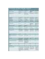
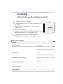
Anexo No. 02.- Datos técnicos del variador de frecuencia.
AF-6 LP™ Micro Drive
AC Adjustable Frequency Drive
Guide-Form Technical
Specification
Contents
1.0
2.0
3.0
4.0
5.0
6.0
7.0
General Information
Operating Conditions
Standards
Input Power Section
Output Power Section
Drive Keypad
Drive Features
AF-60 LP is a trademark of the General Electric Company.
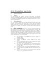
AF-60 LP Guide-Form Specification
1.0
General Information
1.1
Purpose
This specification shall establish minimum requirements for adjustable
frequency drive equipment. Drives that do not meet these requirements shall not
be acceptable. The adjustable frequency drive equipment shall be the AF-60 LP
Micro as furnished by GE.
1.2
Driven Equipment
The Drive shall be capable of operating a NEMA design B squirrel cage
induction motor with a full load current equal to or less than the continuous
output current rating of the Drive. At base speed (60Hz) and below, the Drive
shall operate in a constant V/Hz mode or a constant voltage extended frequency
mode.
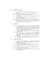
1.3
Drive Construction
The AF-60 LP Adjustable Frequency Drive shall be a sinusoidal PWM type
Drive with sensor-less dynamic torque vector control (DTVC) capability. The
Drive shall be provided in an IP20 enclosure at all ratings. IP21 & NEMA 1
enclosure rating Option Kits shall be available to meet Drive enclosure integrity
requirements. The Drive shall be of modular construction for ease of access to
control and power wiring as well as Maintenance requirements. The Drive shall
consist of the following general components:
1.3.1
1.3.2
1.3.3
1.3.4
1.3.5
1.3.6
1.3.7
1.3.8
Full-Wave Diode Rectifier Bridge to convert AC supply to a
fixed DC voltage
DC link capacitors
Insulated Gate Bipolar Transistor (IGBT) inverter output
section
The Drive shall be microprocessor based with an LCD display
to program and monitor Drive parameters.
The keypad shall be divided into four (4) functional groups:
Numeric Displays, Menu Key, Navigation Keys, and Operation
Keys and LED’s.
Separate control and power terminal boards shall be provided.
The Drive shall provide an RS-485 serial communications port
standard.
The Drive control and power circuit boards shall be conformal
coated for long-life and clean connections.
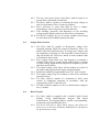
2.0
Operating Conditions
2.0.1 The Drive’s operating ambient temperature range shall be 10°C to 50°C.
2.0.2 The Drive’s storage temperature shall be -25° to 65°C.
2.0.3 The Drive’s relative humidity range shall be 5-95%, noncondensing.
2.0.4 The Drive shall be suitable for operation at altitudes up to 3,280
feet without de-rating.
2.0.5 The Drive shall be capable of sustaining a 1.0g vibration test.
2.0.6 The Drive shall be capable of side-by-side installation
mounting with 0 inches clearance required. The top and bottom
clearance shall be 3.4 inches minimum.
3.0
Standards
3.0.1
The Drive shall be UL and cUL listed and not require any
external fusing. The Drive shall also be CE labeled and comply
with standards 61800-3 for EMC Compliance and EN 61800-2
for Low Voltage Compliance. The Drive shall also be RoHs
Compliant as well as WEEE Compliant.
3.0.2 The Drive shall be designed in accordance with applicable
NEMA Standards.
3.0.3 The Drive shall be compatible with the installation
requirements of interpretive Codes such as National Electric
Code (NEC) and the Occupational Safety & Health Act
(OSHA).
3.0.4 The Drive with standard built-in A1/B1 Filter shall
significantly reduce Radio Frequency Interference (RFI).
4.0
Input Power Section
4.0.1
4.0.2
4.0.3
4.0.4
4.0.5
The Drive shall be designed to operate at either 200-240Vac
Single-Phase or Three-Phase input voltage, or 380-480Vac
Three-Phase input voltage.
System frequency shall be 50 or 60 Hertz, +/- 5%
The Drive shall be able to withstand input voltage variation of
+/- 10%
The Drive shall operate with an input voltage imbalance of
3.0% maximum between phases.
The displacement power factor of the Drive shall be greater
than 0.98 lagging.
4.0.6
The true (real) power factor of the Drive shall be equal to or
greater than 0.4 nominal at rated load.
4.0.7 The Drive shall be capable of switching the input voltage on
and off a maximum of two (2) times per minute.
4.0.8 Drive efficiency at rated load shall be 98% or higher,
depending on carrier frequency selection and load.
4.0.9 Line notching, transients, and harmonics on the incoming
voltage supply shall not adversely affect Drive performance.
4.0.10 The Drive is suitable for use on circuits capable of delivering
no more than 100,000 RMS symmetrical amps.
5.0
Output Power Section
5.0.1
5.0.2
5.0.3
5.0.4
5.0.5
5.0.6
5.0.7
6.0
The Drive shall be capable of Horsepower ratings from
fractional through 10HP and Output Frequencies from 0 to
400Hz. The Drive shall also have an energy saver feature with
the capability of selecting a V/Hz Automatic Control Function
that will modify the V/Hz curve based on load conditions that
will minimize power used.
Drive output voltage shall vary with frequency to maintain a
constant V/Hz ratio up to base speed (60Hz) output. Constant
or linear voltage output shall be supplied at frequencies greater
than base speed (60Hz).
The output voltage of the Drive will be capable of 0-100% of
the input voltage applied at the input voltage terminals.
Ramp times shall be programmable from 0.05-3,600 seconds.
The output voltage may be switched on and off an unlimited
amount of times.
The Drive shall be capable of a minimum of 100% rated
current in continuous operation in accordance with the
requirements of NEC Table 430-150.
The Drive shall be capable of 150% overload current rating for
one (1) minute.
Drive Keypad
6.0.1
6.0.2
The Drive shall be supplied with a backlit Liquid Crystal
Display (LCD) Multi-Function Keypad with Speed
Potentiometer. The Keypad shall be capable of programming,
monitoring, and controlling the Drive.
The Drive shall have a Quick Menu feature, that allows for
quick access to the most commonly modified Drive Parameters
for quick and easy setup.
6.0.3
6.0.4
6.0.5
6.0.6
6.0.7
6.0.8
6.0.9
7.0
The Drive LCD Keypad Display shall have the following units
available for display functions: Hz, A, V, kW, HP, %, s, or
RPM.
The Drive LCD Keypad Display shall have a Motor Direction
Display that will show either clockwise or counter-clockwise
motor direction.
The Drive shall be capable of being operated in “hand” mode
via the keypad to allow for local control of the motor at the
Drive.
The Drive Keypad shall have three (3) Indication LED’s as
follows:
6.0.6.1 Green – The Drive is “on”
6.0.6.2 Yellow – The Drive has an alarm “warning”
6.0.6.3 Red – The Drive has an “alarm”
The Drive shall display operating data, fault information, and
programming parameters.
The Drive LCD Keypad shall be remote mountable by using an
option kit which will allow for mounting the LCD Keypad up
to 10’ from the Drive.
The Drive LCD Keypad shall be capable of copying the
parameter set from one AF-6 LP Micro Drive to another AF-6
LP Micro Drive.
Drive Features
7.0.1
7.0.2
7.0.3
7.0.4
7.0.5
7.0.6
The Drive shall be capable of remote mounting with simple
wiring connections or via an RS-485 serial communications
port.
Upon a fault condition, the Drive shall display drive
parameters captured at the time the fault occurred to aid in
trouble-shooting of the fault. The Drive will store the last ten
(10) fault trips in a Fault Log Parameter.
The Drive shall operate as an open-loop system requiring no
motor fdbk device.
The Drive shall accept and follow a selectable external
frequency reference of 0-10Vdc, 0-20ma, or 4-20mA.
The Drive will also follow an internal frequency set-point off
the up and down arrows on the LCD Keypad, optional LCD
Keypad Speed Potentiometer, parameter preset speeds, or serial
communications speed set-point via RS-485.
The Drive shall maintain the output frequency to within 0.2%
of reference when the reference is analog, and to within 0.01%
of reference when the reference is digital (keypad, contact
closure, or serial communications)
7.0.7
7.0.8
7.0.9
The Drive shall maintain set-point frequency regardless of load
fluctuations.
The Drive shall be able to operate in three (3) modes: Hand,
Off, or Auto.
The Drive shall be password protected to protect against
unintended change of sensitive parameters.
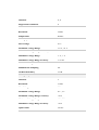
Anexo No. 03. - Datos técnicos de la tarjeta de adquisición de datos.
NI USB-6008
14-Bit, 48 kS/s Low-Cost Multifunction DAQ
• 8 analog inputs (14-bit, 48 kS/s)
• 2 analog outputs (12-bit, 150 S/s); 12 digital I/O; 32bit counter
• Bus-powered for high mobility; built-in signal
connectivity
• OEM version available
• Compatible with LabVIEW, LabWindows/CVI, and
Measurement Studio for Visual Studio .NET
• NI-DAQmx driver software and NI LabVIEW
SignalExpress LE interactive data-logging software
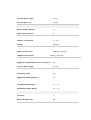
Specifications Summary
General
Product Name
USB-6009
Product Family
Multifunction Data Acquisition
Form Factor
USB
Operating System/Target
Windows , Linux , Mac OS , Pocket
PC
DAQ Product Family
B Series
Measurement Type
Voltage
RoHS Compliant
Yes
Analog Input
Channels
8,4
Single-Ended Channels
8
Differential Channels
4
Resolution
14 bits
Sample Rate
48 kS/s
Throughput
48 kS/s
Max Voltage
10 V
Maximum Voltage Range
-10 V , 10 V
Maximum Voltage Range Accuracy
138 mV
Minimum Voltage Range
-1 V , 1 V
Minimum Voltage Range Accuracy
37.5 mV
Number of Ranges
8
Simultaneous Sampling
No
On-Board Memory
512 B
Analog Output
Channels
2
Resolution
12 bits
Max Voltage
5V
Maximum Voltage Range
0V,5V
Maximum Voltage Range Accuracy
7 mV
Minimum Voltage Range
0V,5V
Minimum Voltage Range Accuracy
7 mV
Update Rate
150 S/s
Current Drive Single
5 mA
Current Drive All
10 mA
Digital I/O
Bidirectional Channels
12
Input-Only Channels
0
Output-Only Channels
0
Number of Channels
12 , 0 , 0
Timing
Software
Logic Levels
TTL
Input Current Flow
Sinking , Sourcing
Output Current Flow
Sinking , Sourcing
Programmable Input Filters
No
Supports Programmable Power-Up States?
No
Current Drive Single
8.5 mA
Current Drive All
102 mA
Watchdog Timer
No
Supports Handshaking I/O?
No
Supports Pattern I/O?
No
Maximum Input Range
0V,5V
Maximum Output Range
0V,5V
Counter/Timers
Counters
1
Buffered Operations
No
Debouncing/Glitch Removal
No
GPS Synchronization
No
Maximum Range
0V,5V
Max Source Frequency
5 MHz
Minimum Input Pulse Width
100 ns
Pulse Generation
No
Resolution
32 bits
Timebase Stability
50 ppm
Logic Levels
TTL
Physical Specifications
Length
8.51 cm
Width
8.18 cm
Height
2.31 cm
I/O Connector
Screw terminals
Related Information
• NI USB Data Acquisition for OEM
• Download NI Data Acquisition Drivers
• NI LabVIEW SignalExpress Interactive Data-Logging Software
© 2010 National Instruments Corporation. All rights reserved. For information
regarding NI trademarks, see ni.com/trademarks. Other product and company names
are trademarks or trade names of their respective companies. Except as expressly set
forth to the contrary below, use of this content is subject to the terms of use for
ni.com.
National Instruments permits you to use and reproduce the content of this model
page, in whole or in part; provided, however, that (a) in no event may you (i) modify
or otherwise alter the pricing or technical specifications contained herein, (ii) delete,
modify, or otherwise alter any of the proprietary notices contained herein, (iii) include
any National Instruments logos on any reproduction, or (iv) imply in any manner
affiliation by NI with, or sponsorship or endorsement by NI of, you or your products
or services or that the reproduction is an official NI document; and (b) you include
the following notice in each such reproduction:
“This document/work includes copyrighted content of National Instruments. This
content is provided “AS IS” and may contain out-of-date, incomplete, or otherwise
inaccurate information. For more detailed product and pricing information, please
visit ni.com.”
http://www.ni.com/niweek/?metc=mtxrhy
Anexo No. 04.- Datos técnicos del Medidor de Energía.
The 3710 ACM is an economical, panel mounted, 3-phase digital power
monitoring instrument. Well established and successful, the 3710 ACM offers
high accuracy, reliability and exceptional ruggedness. It is an affordable
solution for power utilities and industrial or commercial power distribution
systems. The 3710 ACM can be used stand alone or as one element in a large
energy management network. The 3710 ACM is an economical, panel mounted,
3-phase digital power monitoring instrument. Well established and successful,
the 3710 ACM offers high accuracy, reliability and exceptional ruggedness. It
is an affordable solution for power utilities and industrial or commercial power
distribution systems. The 3710 ACM can be used stand alone or as one element
in a large energy management network.
Cost Effective
• Replaces dozens of separate meters
• Simple installation
Measurements
• True RMS voltage, current & power
Data Logging
• Waveform Capture
• Scheduled or event-driven logging
• Min/Max logging
• Sequence of events logging
Extensive I/O
• digital/counter inputs
• 3 digital relay outputs
Powerful Setpoint Control System
• Setpoint on any parameter or condition
Communications
• Supports Modbus, DNP and PLC/AB
Front Panel Display
The front panel features an easy-to-read, 20-character vacuum fluorescent
display. Voltage, current and power functions can all be displayed together for
the selected phase. Voltage or current readings can be displayed for all three
phases concurrently.
The 3710 ACM may also be ordered with no front panel display for use as a
digital power transducer.
• Four sealed membrane switches for parameter selection and programming
• Select voltage and current readings using the PHASE key
• Common power functions are available using the FUNCTION key
• Display the maximum and minimum values for each measured parameter
using the MAX/MIN keys
• Programming and control is password protected
Extensive I/O
Use the inputs to monitor utility KYZ initiators, device cycles, running hours,
etc. Outputs can be used for equipment control, alarms, etc.
Status Inputs
• Four optically isolated, digital (status) inputs can monitor status, count pulses,
or any other external dry contact
Relays
• 3 on-board relays controlled automatically by the internal setpoints or
manually via a communications port
• Programmable for kWh, kVARh or kVAh output pulsing
• Form C mechanical relays rated at 10 A (AC or DC); or single-pole, singlethrow solid state relays rated at 1 A (AC only)
Auxiliary Output
• Auxiliary analog current output provides 0-20mA or 4-20 mA proportional to
any measured parameter
Control
The 3710 ACM setpoint system provides intelligent logging and control
functions.
Programmable Setpoint Control
Setpoints are defined by independent high and low trigger limits (for
operate/release hysteresis), and time delays on both operate/ release for the
resulting function. Multiple setpoints can be channelled to a single relay ("OR"
function) for multi-level setpoint protection functions. All setpoint activity is
recorded automatically in the on-aboard Event Log.
•
•
17 setpoints, one second (typ.) response time
Any setpoint condition can be set to control relays
Metering
The 3710 ACM provides high accuracy true RMS measurements of voltage,
current, power and energy readings, as well as minima, maxima, and status
parameters. All parameters are quickly accessible via the front panel display
or through the communications port. Voltage, current, power and energy
readings are sensitive to beyond the 50th harmonic. Four-quadrant readings
measure bidirectional (import/ export) energy flow, useful in any cogeneration
application.
Instantaneous
Voltage (l-l/l-n), per phase & average
Current, per phase & average
Neutral Current
Real, Reactive & Apparent Power, total (per phase available via
communications)
Power Factor, total
Frequency
Auxiliary Voltage
Phase Reversal
Energy
Real & reactive, imported, exported, total and net kWh & kVARh. Apparent
energy, total kVAh.
Demand
Sliding Window Demand calculated for average current and total real power,
or for total apparent power and total real power.
Minimums and Maximums
Recorded for all base measurements & Sliding Window Demand values.
Logging & Recording
The 3710 ACM provides three types of onboard data logging: events,
min/max levels, and snapshot readings are all automatically time-stamped and
recorded in non-volatile memory. There is also a waveform capture feature.
All logging functions are continuous
and concurrent.
Using Power Measurement.s software you can display all logged data. The
software will automatically archive to disk all logged data retrieved from each
device. The data can be converted to file formats compatible with other
software. Min/max values can also be viewed via the front panel.
Historical Logging
Produce daily/weekly/monthly load profile graphs for important readings.
•
Log up to 12 channels of time-stamped data: V avg, I avg, kW total,
kVAR total, kW total Demand, I avg Demand, PF, Vaux, Frequency,
kWh import, kWh export, and kVARh total
•
Trigger at specified time intervals, 1 second to 400 days for preset &
programmable logs
Minimum/Maximum Logging
Records extreme values for system operations analysis, troubleshooting and
problem tracking.
•
•
Records extreme values for all measured parameters
Minima/maxima for each parameter are logged independently with a
date and time stamp @ 1 second resolution
Event Logging & Alarming
Records all setpoint/alarm conditions, relay operations, setup changes, and
selfdiagnostic events.
•
•
•
The 3710 ACM stores up to 50 date & time stamped records
Time stamp resolution to 1 second
Sequence-of-event recording
Communications
The 3710 ACM can be integrated within energy monitoring networks and
supports a variety of protocols. Links between remote sites can use RS-485 or
modems with telephone lines (dedicated or dial-up), fiber optic and/or radio
links.
Optional Communications Port
•
•
•
•
Single optically isolated, transient protected port
Data rates up to 19,200 bps.
RS-232 or RS-485
PML, A-B DF1, Modicon Modbus RTU or Alarm Dialer protocols
The Alarm Dialer (AD) communication protocol enables the 3710 ACM to
automatically contact a master display station on the occurrence of an alarm
condition.
Input & Output Ratings
Voltage Inputs
•
•
•
•
Basic: 120 line-to-neutral / 208 line-to-line nominal full scale input
277 Option: 277 VAC nominal full scale input
347 Option: 347 VAC nominal full scale input
All options: Overload withstand: 1500 VAC continuous, 2500 VAC
for 1 second. Input impedance for all options: 2 MW
Current Inputs
•
•
•
•
•
•
Basic: 5.0 Amps AC nominal full scale input
1AMP Option: 1.0 Amp AC nominal full scale
All options: Overload withstand 15 Amps continuous, 300 Amps for 1
second. Input impedance: 0.002W
Burden: 0.05 VA Aux. Voltage Input
VAC/VDC nominal full scale input (1.25 VAC /VDC max.) Overload
withstand: 120 VAC/ VDC continuous, 1000 VAC/VDC for 1 second.
Input impedance: 10 kW
Aux. Current Output
•
0 to 20 mA into max. 250W load. Accuracy: 2%
Control Relays
•
•
Basic: Form C dry contact electromechanical relays, max. 277 VAC or
30 VDC @ 10 Amp resistive
SSR Option: SPST solid state relays, 24 to 280 VAC @ 1 Amp AC
resistive (AC operation only)
Status Inputs
•
•
•
•
Basic: external-excited, S1, S2, S3, S4 - >20 VAC/VDC = active, <6
VAC/VDC = inactive
Input impedance: 49.2 kW Overload withstand: 1500 V continuous,
2500 V for 1 sec.
SES Option: self-excited +30 VDC differentialSCOM output to S1,
S2, S3, or S4 input
All Options: Minimum Pulse Width: 40 msec.
Power Supply
•
Basic: 85 to 132 VAC / 47 to 440 Hz or 110 to 170 VDC @ 0.2 Amps
•
•
P24/48 Option: 20 to 60 VDC @ 10W
P240 Option: 85 to 264 VAC / 47 to 440 Hz or 110 to 340 VDC / 0.2
A
Environmental Conditions
Operating Temp: 0oC to 50oC (32oF to 122oF) ambient air
(XTEMP Option): -20oC to +70oC (-4oF to +158oF)
Storage Temp: -30oC to +70oC (-22oF to +158oF)
Humidity: 5 to 95 %, non-condensing
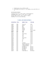
TABLA DE REGISTROS
REGISTRO TIPO
DIRECCION
UNIDAD
40002
40003
40004
40005
40006
40007
40008
40011
40012
40013
40014
40015
40016
40017
40018
40020
40021
40022
40023
40024
40026
40028
40029
40031
40032
40033
40034
40035
Year year
Month
Day
Hour
Minute
Second
UNIX
Van
Vbn
Vcn
Vln average
Vab
Vbc
Vca
Vll average
Vaux
Ia
Ib
Ic
I average
Neutral current (I4)
Voltage imbalance
Current imbalance
kW Phase A
kW Phase B
kW Phase C
kW Total
kVAR Phase A
1900
(1-12)
(1-31)
(0-23)
(0-59)
(0-59)
Time seconds
V rms
V rms
V rms
V rms
V rms
V rms
V rms
V rms
V rms
A rms
A rms
A rms
A rms
A rms
%
%
kW rms
kW rms
kW rms
kW rms
kVAR rms
RW
RW
RW
RW
RW
RW
RW
RO
RO
RO
RO
RO
RO
RO
RO
RO
RO
RO
RO
RO
RO
RO
RO
RO
RO
RO
RO
RO
40036
40037
40038
40039
40040
40041
40042
40043
40044
40045
40046
40048
40049
40050
40051
40052
40053
40054
40055
40056
40057
40058
40061
40062
40063
40064
40065
40066
40067
40068
40071
40072
40073
40074
40075
40076
40077
40078
RO
RO
RO
RO
RO
RO
RO
RO
RO
RO
RO
RO
RO
RO
RO
RO
RO
RO
RO
RO
RO
RO
RO
RO
RO
RO
RO
RO
RO
RO
RO
RO
RO
RO
RO
RO
RO
RO
kVAR Phase B
kVAR rms
kVAR Phase C
kVAR rms
kVAR Total
kVAR rms
Power Factor Phase A
%
Power Factor Phase B
%
Power Factor Phase C
%
Power Factor Total
%
kVA Phase A
kVA
kVA Phase B
kVA
kVA Phase C
kVA
kVA Total
kVA
Frequency on Va
0.01 Hz
Phase Reversal Logical
Real time polarity Bit mapped
kWh Import kWh
M/GWh Import
M/GWh
kWh Export
kWh
M/GWh Export
M/GWh
kWh Total
kWh
M/GWh Total
M/GWh
kWh Net
kWh
M/GWh Net
M/GWh
kVARh Import
kVARh
M/GVARh Import M/GVARh
kVARh Export
kVARh
M/GVARh Export M/GVARh
kVARh Total
kVARh
M/GVARh Total
M/GVARh
kVARh Net
kVARh
M/GVARh Net
M/GVARh
kVAh Import
kVAh
M/GVAh Import
M/GVAh
kVAh Export
kVAh
M/GVAh Export
M/GVAh
kVAh Total
kVAh
M/GVAh Total
M/GVAh
kVAh Net
kVAh
M/GVAh Net
M/GVAh
Worldwide Headquarters
Power Measurement Ltd.2195 Keating Cross Road,
Saanichton, British Columbia, Canada V8M 2A5
Tel: 1-250-652-7100 Fax: 1-250-652-0411
Web: www.pml.com Email: [email protected]
Anexo No. 05.- Datos técnicos del Convertidor de Protocolo.
Model 485SD9TB
Port-Powered RS-485 Converter
The 485SD9TB is a port-powered two-channel RS-232 to RS-485 converter. It
converts the TD and RD RS-232 lines to balanced half-duplex RS-485 signals.
The unit is powered from the RS-232 data and handshake lines whether the lines
are high or low. An external power supply can be connected to two terminals on
the RS-485 connector if no handshake lines are available. The 485SD9TB has a
DB-9 female connector on the RS-232 side and a terminal block connector on the
RS-485 side.
RS-232 Side:
Connector: DB-9 Female.
Signals: Passes through pins 3 (TD) and 2 (RD).
Pins 7 (RTS) and 8 (CTS) are tied together.
Pins 4 (DTR), 6 (DSR), and 1 (CD) are tied together.
RS-485 Side:
Connector: Terminal Block
Signals: Half-duplex two-wire operation only.
Automatic control circuit enables driver only when transmitting.
Receiver is disabled when transmitting to prevent echo back to RS-232 device.
Can transmit up to 4000 feet at 115.2k baud.
Power Requirements
No external power required if two RS-232 output handshake lines are available.
External 12VDC can be applied to pins on the RS-485 side between terminals
+12VDC and GND if handshake lines are not available.
35mA current draw maximum under normal operation when externally powered.
NOTE: When using an external supply, the supply should be connected only
to specifically labeled power inputs (power jack, terminal block, etc.).
Connecting an external power supply to the handshake lines may damage the
unit. Contact technical support for more information on connecting an
external power supply to the handshake lines.
Dimensions: 3.50 x 1.34 x .67 in (8.9 x 3.4 x 1.7 cm)
Although the 485SD9TB uses handshake lines to power the converter, no
handshaking is required to control the RS- 485 driver. The RS-485 driver is
automatically enabled during each spacing state on the RS-232 side. During the
marking or idle state, the RS-485 driver is disabled and the data lines are held in
the marking state by the 4.7K ohm pull-up and pull-down resistors. The value of
these resistors may need to be changed to a different value when termination is
used in order to maintain the proper DC bias during the idle state. See B&B
Electronics’ RS-422/RS-485
Application Note for more information on termination and DC biasing of an RS485 network. The 485SD9TB has an internal connection to prevent data
transmitted from the RS-232 port from being echoed back to the RS-232 port. The
485SD9TB is used as a two wire (half duplex) RS-485 converter.
International Headquarters:
707 Dayton Road P.O. Box 1040 Ottawa, IL 61350 USA
815-433-5100 Fax 433-5104 www.bb-elec.com [email protected] [email protected]
Westlink Commercial Park Oranmore Co. Galway Ireland
+353 91 792444 Fax +353 91 792445 www.bb-europe.com [email protected] [email protected]
Anexo No. 06.- LABORATORIOS.
Laboratorio No. 01.- Identificación de Sistemas por el Método No
Pàrametrico.
Laboratorio No. 02.- Identificación de Sistemas por el Método
Paramétrico.
Laboratorio No. 03.- Diseño de Control para la Planta Identificada.
Laboratorio No. 04.- Programación del Control Adaptativo de Ganancia
Programada.
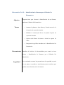
Laboratorio No. 01.- Identificación de Sistemas por el Método No
Pàrametrico.
Objetivo
Capturar datos para efectuar la Identificación de un Sistema,
mediante el Método No Paramétrico.
Tareas
•
Arrancar la planta en lazo abierto y llevarla cerca, de la
frecuencia de operación deseada.
•
Habilitar el control para llevar a la planta al punto de
operación deseado.
•
Aplicar ruido blanco al sistema e iniciar la captura de
datos.
•
Interpretar los gráficos obtenidos en la Identificación No
Paramétrica.
Herramientas Pantallas de Labview 8.6 desarrolladas para control en lazo
abierto e Identificación de Sistemas, por el Método No
Paramétrico.
Seguridad
Se recomienda extremar las precauciones de seguridad, a partir
de este punto, se podrán en movimiento partes mecánicas que
podrían causar lesiones serias ó la muerte.
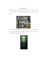
DESARROLLO
1. Energizar la Planta con una fuente de energía trifásica, 230 voltios, 60 Hz, y
cerrar los disyuntores de protección principal que están dentro del tablero de
control.
2. Poner el variador de frecuencia en automático, a partir de este punto el equipo
puede ser arrancado desde el computador sin previo aviso, por lo que se
recomienda tener las precauciones del caso.
3. Arrancar desde el computador el archivo Tesis01 que ha sido desarrollado para el
control de la Planta, con el software Labview 8.6.
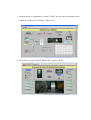
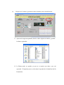
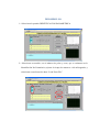
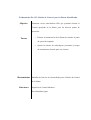
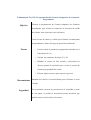
4. Seleccionar la pestaña PANEL PRINCIPAL y pulsar “RUN”
5.
Arrancar la planta accionando el Interruptor de ARRANQUE REMOTO. Desde
esta pantalla se monitorearán varios parámetros del variador de frecuencia.
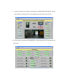
6. Al seleccionar la pestaña ALTERNADOR, se puede monitorear los parámetros del
generador.
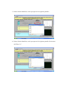
7. Seleccionar la pestaña SISTEMA EN LAZO ABIERTO, para activar esta pantalla
pulsar el botón Habilitar.
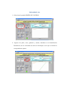
8. Incrementar la referencia hasta obtener la frecuencia de salida deseada de la
Planta.
Recuerde los puntos de interés para este sistema, están ubicados a 50, 52, 54,
56, 58 y 60 Hz. Finalmente solo se seleccionarán 6 Funciones de
Transferencia, que representaran el rango de frecuencia de interés, que se
requiere controlar en este sistema.
Al efectuar la Identificación en un punto, por ejemplo 56 Hz y puesto que el
sistema será excitado para generar variaciones de +- 1 Hz, la Función de
Transferencia que se obtendrá, servirá para representar la dinámica del
sistema dentro del rango 56Hz +- 1Hz.
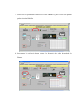
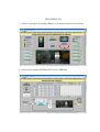
9. En este momento se ha fijado como punto de operación de la Planta 60 Hz, si se
desea otro punto de operación variar la referencia. A partir de este punto podemos
iniciar el proceso de excitación de la entrada con ruido blanco al mismo tiempo, se
comenzará a guardar datos para la Identificación.
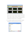
10.
Después de 2 minutos, guardar los datos tomados para la Identificación.
11. Aparecerá la siguiente pantalla, donde se debe asignar un nombre y guardar
los datos registrados.
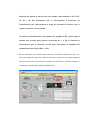
12. La Planta puede ser parada, ya que no se requiere por ahora que esté
operando. El siguiente paso es seleccionar la pestaña de la Identificación No
Paramétrica.
Debemos seleccionar en la Fuente de datos “Load from file”, además se debe
indicar el número de muestras estimadas, considerando que el programa
removió la media y las tendencias de las muestras. También debe tenerse en
consideración que el tiempo de muestreo es de 60 milisegundos.
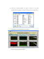
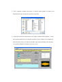
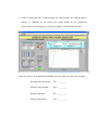
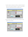
13. Una vez ajustados estos parámetros, pulsar el botón Identificar, la siguiente
ventana aparecerá, seleccionar el tipo de archivo por “All Files(*,*)”
14. Aparecerá la siguiente pantalla, con todos los archivos con los datos
grabados, para este ejemplo se tomarán, los datos a 60 Hz y se pulsara OK.
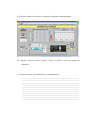
15. Se obtendrán las siguientes respuestas del Sistema.
En base a los gráficos obtenidos indicar:
PARA LA RESPUESTA A UNA ENTRADA ESPECIAL
a. ¿Cuál es el orden del modelo, que representaría este sistema ante la
entrada tipo escalón ?.
___________________________________________________________
___________________________________________________________
___________________________________________________________
b. El sistema es:
Subamortiguado
Criticamente amortiguado
Sobreamortiguado
______
______
______
c. ¿Cuál es la ganancia en estado estacionario?.
___________________________________________________________
___________________________________________________________
___________________________________________________________
d. ¿En qué tiempo aproximadamente el sistema alcanza el valor nominal?.
___________________________________________________________
___________________________________________________________
___________________________________________________________
e. ¿Qué nos indica el espectro de potencia de la señal de entrada?.
___________________________________________________________
___________________________________________________________
___________________________________________________________
ANALISIS DE CORRELACION
f. ¿Cuál es el comportamiento del sistema ante la señal impulso aplicada?.
___________________________________________________________
___________________________________________________________
___________________________________________________________
g. ¿Hay algún retardo de tiempo?.
___________________________________________________________
___________________________________________________________
___________________________________________________________
h. Con el nivel de autocorrelación que se obtuvo es suficiente, para capturar
la dinámica del sistema?.
___________________________________________________________
___________________________________________________________
___________________________________________________________
ANALISIS ESPECTRAL
i. En base al gráfico de magnitud y fase de este sistema, calcule el margen
de ganancia y margen de fase.
___________________________________________________________
___________________________________________________________
___________________________________________________________
_________________________________________________________________
________________________________________________________________
________________________________________________________________
j. Según la respuesta de fase ¿Cuál es el mínimo número de polos y ceros,
que representa este sistema?.
___________________________________________________________
___________________________________________________________
___________________________________________________________
16. Proceda a anotar las conclusiones y recomendaciones:
____________________________________________________________________
____________________________________________________________________
____________________________________________________________________
____________________________________________________________________
____________________________________________________________________
____________________________________________________________________
____________________________________________________________________
____________________________________________________________________
____________________________________________________________________
____________________________________________________________________
____________________________________________________________________
____________________________________________________________________
____________________________________________________________________
____________________________________________________________________
____________________________________________________________________
____________________________________________________________________
____________________________________________________________________
____________________________________________________________________
En base a las conclusiones que ha obtenido, efectuar la Identificación
Paramétrica y obtener la ecuación que mejor representa este sistema.
Laboratorio No. 02.- Identificación de Sistemas por el Método
Paramétrico.
Objetivo
Efectuar la Identificación de un Sistema, mediante el Método
Paramétrico, usando los modelos ARX, ARMAX, Output Error.
Box Jenkins ó General Lineal.
Tareas
•
Efectuar la Identificación de la Planta usando los diversos
modelos, variando el número de polos y ceros de los
polinomios característicos, tomando como base la
información
obtenida
en
la
Identificación
No
Paramétrica.
•
Analizar la Autocorrelación, Correlación Cruzada y el
Error obtenido con las diversas Identificaciones.
•
Escoger la función de transferencia que mejor represente
el sistema.
Herramientas Pantallas de Labview 8.6 desarrolladas para la Identificación
Paramétrica.
Literatura
Departamento de Automática y Computación. ISPJAE.
Identificación de Sistemas por Msc. Aristides Reyes Bacardí.
DESARROLLO
1.- Seleccionar la pestaña IDENTIFICACION PARAMETRICA.
2.- Seleccionar un modelo, con el número de polos y ceros, que se estimaron en la
Identificación No Paramétrica, ajustar el tiempo de muestreo a 60 milisegundos y
seleccionar como fuente de datos “Load From File”.
3.- Pulsar el botón Identificar, con lo que aparecerá la siguiente pantalla.
4.- Pulsar el botón Identificar, con lo que aparecerá la siguiente pantalla. Seleccionar
“All Files(*.*)”.
5.- En la siguiente ventana seleccionar, el archivo donde guardo los datos de la
Identificación, para el punto de operación requerido.
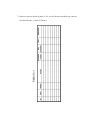
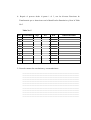
6.- Copiar la Función de Transferencia en la Tabla 4, también debe copiarse, el valor
de la Autocorrelación, la Correlación cruzada y el error. Dentro de la columna de
observaciones, anotar si la función obtenida, representa la dinámica del sistema y
si es posible disminuir el número de polos y ceros.
7.- Repetir el proceso desde el punto 3 al 6, con los diversos modelos que están en
este Identificador, y llenar la Tabla 4.
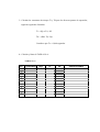
Use la siguiente convención.
ARX 221 equivalente a decir Modelo ARX con 2 polos, 2 ceros y un retardo de tiempo
BJ 321 equivalente a decir Modelo Box Jenskins con 3 polos, 2 ceros y un retardo de tiempo
8.- Una vez que tenga llena la tabla, seleccione la función de transferencia que mejor
representa la dinámica del sistema, para el punto de operación seleccionado. Si se
desea obtener la función de transferencia para otros puntos de operación, se debe
repetir el proceso.
9.- Anote las funciones de Transferencia obtenidas para los diversos puntos de
operación.
Para 50 Hz. G1(s)= ________________________________
Para 52 Hz. G2(s)= ________________________________
Para 54 Hz. G3(s)= ________________________________
Para 56 Hz. G4(s)= ________________________________
Para 58 Hz. G5(s)= ________________________________
Para 60 Hz. G6(s)= ________________________________
10.- Proceda a anotar las conclusiones y recomendaciones:
____________________________________________________________________
____________________________________________________________________
____________________________________________________________________
Laboratorio No. 03.- Diseño de Control para la Planta Identificada.
Objetivo
Sintonizar varios controladores PID, que permitan efectuar el
Control apropiado de la Planta, para los diversos puntos de
operación.
Tareas
•
Efectuar la sintonización de la Planta de acuerdo al punto
de operación asignado.
•
Ajustar los límites de sobredisparo porcentual y tiempo
de asentamiento deseado para este sistema.
Herramientas Pantallas de Labview 8.6 desarrolladas para el Diseño de Control
de la Planta.
Literatura
Ingeniería de Control Moderna
Por: Katsuhiko Ogata.
DESARROLLO
1.- Seleccionar la pestaña DISEÑO DE CONTROL.
2.- Ingresar los polos, ceros, ganancia y retardo, obtenidos en la Identificación
Paramétrica, una vez efectuado esto activar el interruptor, con lo que se inician los
correspondientes ajustes.
3.- Como se puede apreciar, se deben ajustar los valores de Kp, Ki y Kd para que el
sistema, se comporte de tal manera que quede dentro de los parámetros
seleccionados de sobredisparo porcentual y tiempo de asentamiento deseado.
Copie los valores de las ganancias obtenidas para este punto de operación escogido.
Frecuencia de Operación:
Hz = _________.
Ganancia proporcional:
Kp = _________.
Ganancia Integral:
Ki = _________.
Ganancia Derivativa:
Kd = _________.
4.- Repetir el proceso desde el punto 1 al 3, con las diversas Funciones de
Transferencia que se obtuvieron con la Identificación Paramétrica y llene la Tabla
No.5.
Tabla No. 5
No. Frecuencia
Kp.
Ki.
Kd.
Observaciones
1
2
3
4
5
5.- Proceda a anotar las conclusiones y recomendaciones:
____________________________________________________________________
____________________________________________________________________
____________________________________________________________________
____________________________________________________________________
____________________________________________________________________
____________________________________________________________________
____________________________________________________________________
____________________________________________________________________
____________________________________________________________________
____________________________________________________________________
____________________________________________________________________
____________________________________________________________________
Laboratorio No. 04.- Programación del Control Adaptativo de Ganancia
Programada.
Objetivo
Efectuar la programación del Control Adaptativo de Ganancia
Programada, para efectuar el control de la frecuencia de salida
del sistema, ante variaciones en la referencia.
Cerrar el lazo de control y verificar que la Planta, está trabajando
apropiadamente, dentro del rango de operación establecido.
Tareas
•
Llenar la tabla de ganancias programadas obtenidas en el
Laboratorio No. 03,
•
Calcular las constantes de tiempo Ti y Td.
•
Habilitar el control en lazo cerrado y seleccionar los
diversos puntos de operación para el cual el control de
Ganancia programada fue creado.
•
Efectuar ajustes menores para mejorar el proceso.
Herramientas Pantallas de Labview 8.6 desarrolladas para el Sistema en Lazo
Cerrado.
Seguridad
Se recomienda extremar las precauciones de seguridad, a partir
de este punto, se podrán en movimiento partes mecánicas que
podrían causar serias lesiones ó la muerte.
DESARROLLO
1.- Active el interruptor de arranque Remoto y Arranque la planta en lazo abierto.
2.- Seleccionar la pestaña SISTEMA EN LAZO CERRADO.
3.- Calcular las constantes de tiempo Ti y Td para los diversos puntos de operación,
según las siguientes formulas:
Ti = (Kp x Ts) / Ki
Td = (Kd x Ts) / Kp
Considere que Ts = 0,060 segundos.
4.- Calcular y llenar la TABLA No. 6.
TABLA No. 6
No. Frecuencia
1
2
3
4
5
Kp.
Ti.
Td.
Observaciones
5.- Llenar la tabla de Ganancias Programadas, según los datos obtenidos en el
Laboratorio No. 03.
6.- Activar el control y cerrar el lazo, pulsando el botón de habilitar.
7.- Ajustar la referencia a un valor entre 50 y 60 Hz en la ventana F.R., usted podrá
apreciar como la frecuencia de salida sigue a la referencia. En forma análoga,
seleccionar el comportamiento del sistema al variar dicha referencia.
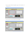
8.- Oscilar la referencia usando el botón Aplicar variación, el cual aplicara un paso
escalón de 1 Hz. A la referencia.
9.-El sistema seguirá la referencia y mostrara el siguiente comportamiento.
10.- Repetir el proceso desde el punto 7 hasta el punto 9, para otros puntos de
referencia:
11.- Proceda a anotar las conclusiones y recomendaciones:
____________________________________________________________________
____________________________________________________________________
____________________________________________________________________
____________________________________________________________________
____________________________________________________________________
____________________________________________________________________
____________________________________________________________________
____________________________________________________________________
____________________________________________________________________
____________________________________________________________________
____________________________________________________________________
Bibliografìa
- Msc. Héctor Garcini, “Sistemas de Control en Tiempo Contínuo”, Folleto de
Maestria en Automatizacion y Control Industrial, año 2008 – 2009.
- Dr. Roger Misa Llorca, “Sistemas Discretos”, La Habana – Cuba, Marzo 2007.
- Eduardo F. Camacho y Carlos Bordons, CONTROL PREDICTIVO: PASADO,
PRESENTE Y FUTURO, Escuela Superior de Ingenieros. Universidad de Sevilla,
Octubre 2004.
- Dagoberto Montero, David B. Barrantes y Jorge M. Quirós, Introducción a los
sistemas de control supervisor y de adquisición de datos (SCADA) ,
Monogarafia de Sistema de Control, Universidad de Costa Rica, año 2004.
- National Instrument, Labview PID Control Toolkit User Manual, www.ni.com,
Junio 2008.