Download User manual ()

XMBF 2.40
Stefan Meinel
June 7, 2013
Contents
1 Introduction
2 Compiling XMBF
2.1 Standard Double-Precision Build . . .
2.2 Build with Quad-Double Inverter . . .
2.3 Build for parallel bootstrap with MPI
2.4 Additional programs . . . . . . . . . .
3
.
.
.
.
3
3
3
4
4
3 Using XMBF
3.1 Using XMBF_mpack_qd . . . . . . . . . . . . . . . . . . . . . . . . . . . . . . . . . . . . .
3.2 Using XMBF_mpi . . . . . . . . . . . . . . . . . . . . . . . . . . . . . . . . . . . . . . . . .
4
5
5
4 Basic structure of the input file
5
5 The macros node
6
6 The combined_models node
6
.
.
.
.
.
.
.
.
.
.
.
.
.
.
.
.
.
.
.
.
.
.
.
.
.
.
.
.
.
.
.
.
.
.
.
.
.
.
.
.
.
.
.
.
.
.
.
.
.
.
.
.
.
.
.
.
.
.
.
.
.
.
.
.
.
.
.
.
.
.
.
.
.
.
.
.
.
.
.
.
.
.
.
.
.
.
.
.
.
.
.
.
.
.
.
.
.
.
.
.
.
.
.
.
.
.
.
.
7 The chi_sqr_extra_term node
10
8 The fit_settings node
11
9 The parameter_values and constant_values nodes
12
10 More details on fit ranges
14
10.1 Lower and upper bounds . . . . . . . . . . . . . . . . . . . . . . . . . . . . . . . . . . . . 14
10.2 Step sizes . . . . . . . . . . . . . . . . . . . . . . . . . . . . . . . . . . . . . . . . . . . . 14
11 More details on bootstrap
14
11.1 Resampling the data . . . . . . . . . . . . . . . . . . . . . . . . . . . . . . . . . . . . . . 14
11.2 Resampling both the data and the fit ranges . . . . . . . . . . . . . . . . . . . . . . . . . 15
12 Multifit
16
1
13 Built-in Models
13.1 Scalar two-point models . . . . . . . . . . . . . . . . . .
13.1.1 multi_exp_model . . . . . . . . . . . . . . . . .
13.1.2 multi_exp_expE_model . . . . . . . . . . . . . .
13.1.3 multi_exp_Asqr_model . . . . . . . . . . . . . .
13.1.4 multi_exp_Asqr_expE_model . . . . . . . . . . .
13.1.5 multi_alt_exp_model . . . . . . . . . . . . . . .
13.1.6 multi_alt_exp_expE_model . . . . . . . . . . .
13.1.7 multi_alt_exp_Asqr_model . . . . . . . . . . .
13.1.8 multi_alt_exp_Asqr_expE_model . . . . . . . .
13.2 Vector two-point models . . . . . . . . . . . . . . . . . .
13.3 Two-point models with periodic B.C. . . . . . . . . . . .
13.4 Two-point models with time-independent contributions
13.5 Matrix two-point models . . . . . . . . . . . . . . . . . .
13.5.1 multi_exp_mat_model . . . . . . . . . . . . . . .
13.5.2 multi_exp_expE_mat_model . . . . . . . . . . .
13.5.3 multi_alt_exp_mat_model . . . . . . . . . . . .
13.5.4 multi_alt_exp_expE_mat_model . . . . . . . . .
13.6 Matrix two-point models, type II . . . . . . . . . . . . .
13.6.1 multi_exp_mat_II_model . . . . . . . . . . . . .
13.6.2 multi_exp_expE_mat_II_model . . . . . . . . .
13.7 Triangular matrix two-point models . . . . . . . . . . .
13.7.1 multi_exp_mat_upper_model . . . . . . . . . . .
13.7.2 multi_exp_expE_mat_upper_model . . . . . . .
13.7.3 multi_exp_mat_II_upper_model . . . . . . . . .
13.7.4 multi_exp_expE_mat_II_upper_model . . . . .
13.8 Non-symmetric matrix two-point models . . . . . . . . .
13.8.1 multi_exp_nonsym_mat_model . . . . . . . . . .
13.8.2 multi_exp_expE_nonsym_mat_model . . . . . . .
13.8.3 multi_alt_exp_nonsym_mat_model . . . . . . .
13.8.4 multi_alt_exp_expE_nonsym_mat_model . . . .
13.9 Scalar three-point models . . . . . . . . . . . . . . . . .
13.9.1 threept_multi_exp_model . . . . . . . . . . . .
13.9.2 threept_multi_exp_expE_model . . . . . . . . .
13.9.3 threept_multi_alt_exp_model . . . . . . . . .
13.9.4 threept_multi_alt_exp_expE_model . . . . . .
13.10Vector three-point models . . . . . . . . . . . . . . . . .
13.11“Degenerate” three-point models . . . . . . . . . . . . .
13.11.1 threept_constant_model . . . . . . . . . . . . .
13.11.2 threept_constant_sqr_model . . . . . . . . . .
13.11.3 multi_exp_2var_model . . . . . . . . . . . . . .
13.11.4 multi_exp_expE_2var_model . . . . . . . . . . .
13.12Multi-particle two-point models . . . . . . . . . . . . . .
13.12.1 multi_part_exp_expE_model . . . . . . . . . . .
14 User-defined model
.
.
.
.
.
.
.
.
.
.
.
.
.
.
.
.
.
.
.
.
.
.
.
.
.
.
.
.
.
.
.
.
.
.
.
.
.
.
.
.
.
.
.
.
.
.
.
.
.
.
.
.
.
.
.
.
.
.
.
.
.
.
.
.
.
.
.
.
.
.
.
.
.
.
.
.
.
.
.
.
.
.
.
.
.
.
.
.
.
.
.
.
.
.
.
.
.
.
.
.
.
.
.
.
.
.
.
.
.
.
.
.
.
.
.
.
.
.
.
.
.
.
.
.
.
.
.
.
.
.
.
.
.
.
.
.
.
.
.
.
.
.
.
.
.
.
.
.
.
.
.
.
.
.
.
.
.
.
.
.
.
.
.
.
.
.
.
.
.
.
.
.
.
.
.
.
.
.
.
.
.
.
.
.
.
.
.
.
.
.
.
.
.
.
.
.
.
.
.
.
.
.
.
.
.
.
.
.
.
.
.
.
.
.
.
.
.
.
.
.
.
.
.
.
.
.
.
.
.
.
.
.
.
.
.
.
.
.
.
.
.
.
.
.
.
.
.
.
.
.
.
.
.
.
.
.
.
.
.
.
.
.
.
.
.
.
.
.
.
.
.
.
.
.
.
.
.
.
.
.
.
.
.
.
.
.
.
.
.
.
.
.
.
.
.
.
.
.
.
.
.
.
.
.
.
.
.
.
.
.
.
.
.
.
.
.
.
.
.
.
.
.
.
.
.
.
.
.
.
.
.
.
.
.
.
.
.
.
.
.
.
.
.
.
.
.
.
.
.
.
.
.
.
.
.
.
.
.
.
.
.
.
.
.
.
.
.
.
.
.
.
.
.
.
.
.
.
.
.
.
.
.
.
.
.
.
.
.
.
.
.
.
.
.
.
.
.
.
.
.
.
.
.
.
.
.
.
.
.
.
.
.
.
.
.
.
.
.
.
.
.
.
.
.
.
.
.
.
.
.
.
.
.
.
.
.
.
.
.
.
.
.
.
.
.
.
.
.
.
.
.
.
.
.
.
.
.
.
.
.
.
.
.
.
.
.
.
.
.
.
.
.
.
.
.
.
.
.
.
.
.
.
.
.
.
.
.
.
.
.
.
.
.
.
.
.
.
.
.
.
.
.
.
.
.
.
.
.
.
.
.
.
.
.
.
.
.
.
.
.
.
.
.
.
.
.
.
.
.
.
.
.
.
.
.
.
.
.
.
.
.
.
.
.
.
.
.
.
.
.
.
.
.
.
.
.
.
.
.
.
.
.
.
.
.
.
.
.
.
.
.
.
.
.
.
.
.
.
.
.
.
.
.
.
.
.
.
.
.
.
.
.
.
.
.
.
.
.
.
.
.
.
.
.
.
.
.
.
.
.
.
.
.
.
.
.
.
.
.
.
.
.
.
.
.
.
.
.
.
.
.
.
.
.
.
.
.
.
.
.
.
.
.
.
.
.
.
.
.
.
.
.
.
.
.
.
.
.
.
.
.
.
.
.
.
.
.
.
.
.
.
.
.
.
.
.
.
.
.
.
.
.
.
.
.
.
.
.
.
.
.
.
.
.
.
.
.
.
.
.
.
.
.
.
.
.
.
.
.
.
.
.
.
.
.
.
.
.
.
.
.
.
.
.
.
.
.
.
.
.
.
.
.
.
.
.
.
.
.
.
.
.
.
.
.
.
.
.
.
.
.
.
.
.
.
.
.
.
.
.
.
.
.
.
.
.
.
.
.
.
.
.
.
.
16
16
16
17
17
17
17
18
18
18
19
19
20
22
22
22
23
23
23
24
24
24
24
25
25
25
26
26
26
27
28
28
28
29
29
31
31
32
32
32
32
33
33
33
34
1
Introduction
XMBF is used to perform fits that can combine multiple QMBF-type fit models, each with its
own data file, to a simultaneous, fully correlated fit. See the documentation of QMBF for the
meaning of “QMBF-type fit model” and the data file format. More information on the method of
combining multiple models to a simultaneous correlated fit can be found in Appendix C.2 of the
PhD thesis “Heavy quark physics on the lattice with improved nonrelativistic actions”, available at
http://www.dspace.cam.ac.uk/handle/1810/225126.
In XMBF, fit parameters with the same name across different models will be shared. The parameter names for each model are defined using input from the user, so that the user can decide which
parameters will be common to which fit models. XMBF uses XML input files to specify the models,
fitting ranges etc. The XML files are read such that for each node, the order of the child nodes does
not matter. Comments are also allowed, using the standard XML syntax for comments.
To allow the correct calculation of correlations, the data files for each model must correspond to
the same order of measurements.
2
Compiling XMBF
2.1
Standard Double-Precision Build
Required libraries are
• GNU Scientific Library, version ≥ 1.13
• libxml++
• Boost C++ libraries
and their dependencies. When installing these libraries using a package manager, note that the development packages are also needed (these usually have -dev or -devel in the package name). A
Makefile is supplied with the source code; the variables INCPATH and LIBS may require adjustment for
the specific machine.
2.2
Build with Quad-Double Inverter
It is possible to compile a version of XMBF that uses the libraries
• MPACK Multiple precision arithmetic BLAS (MBLAS) and LAPACK (MLAPACK),
• QD Quad Double package,
to invert the data correlation matrix in “quad double” precision (256 bits, approx. 64 digits). This is
useful to prevent round-off errors when the data correlation matrix has a condition number larger than
1016 . Note that most numerical operations in the quad-double build of XMBF are still performed in
standard double precision; only the inversion (or pseudo-inversion) of the data correlation matrix (and
some related operations) are performed in quad double precision.
To compile this higher-precision version, install MPACK and QD, and then compile XMBF using
the makefile Makefile_mpack_qd (after adjusting the variables INCPATH and LIBS). This generates an
executable called XMBF_mpack_qd.
When doing a fit with XMBF_mpack_qd, if the XML input file specifies the inversion method LU (see
Sec. 12), then MPACK’s functions Rgetrf and Rgetri are used to fully invert the data correlation
3
matrix. If the XML input file instead specifies svd_fixed_cut, svd_ratio_cut, or svd_absolute_cut (see Sec. 12), the MPACK function Rsyev is used to compute the spectral decomposition of the
data correlation matrix, and then the pseudo-inverse, removing the contributions from the smallest
eigenvalues as determined by the user. Note that with version 0.6.7 of MPACK, the function Rsyev
may fail for large matrices (dimension more than about 500) for an unknown reason, in which case
XMBF will abort.
2.3
Build for parallel bootstrap with MPI
It is possible to build a version of XMBF that performs bootstrap (see Sec. 11) in parallel, using MPI.
To compile this version, use make -f Makefile_mpi (after adjusting this Makefile for your machine,
if necessary). This generates an MPI executable called XMBF_mpi. Note that this executable has
restricted functionality (bootstrap only).
2.4
Additional programs
The source of XMBF includes some additional programs for manipulating the XML files. These
programs can be found in subdirectories and must be compiled separately. The most important tool is
called MBF_to_XMBF, and allows to convert .mbf session files generated by QMBF into XML input files
for use with XMBF. The usage is as follows:
MBF_to_XMBF mbf_file xml_file
3
Using XMBF
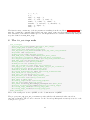
XMBF requires an XML input file containing all the settings, e.g. the fit models, start values for the
parameters, the locations of the data files. The usage is as follows:
XMBF [ options ] inputfile
options :
-o output . xml
-c cov . dat
-r res . dat
- re res_err . dat
-p directory
-b directory
-m directory
-v level
write fit results to " output . xml "
write covariance matrix to " cov . dat "
write results to " res . dat "
write results with errors to " res_err . dat "
plot data and fit functions , write output files to " directory "
perform bootstrap , write output files to " directory "
perform multifit , write output files to " directory "
verbose level [0 ,1 ,2]
XMBF always reads the input file and performs a fit; the results are printed to stdout. When
the option -o outputfile is given, the fit results are additionally written to an output file in XML
format. When the options -c cov.dat is specified, the elements of the parameter covariance matrix
are written to the specified file (similarly, -r res.dat writes the central values of the fitted parameters;
-re res_err.dat writes the central values and errors). With the option -p directory, the averaged
data and the values of the fitted functions are written to files in the specified directory; these files can
then be used for plotting. With the option -b directory, XMBF performs the bootstrap procedure
(see Sec. 11) and writes the results for each parameter into an individual file in directory. With the
option -m directory, XMBF performs the “multifit” procedure (see Sec. 12) and writes the results
for each parameter into an individual file in directory.
4
The option -v level determines how much information is printed to stdout during the fit. The
default corresponds to -v 0. With -v 1, after every iteration the current values of χ2 /dof and λ are
printed; with -v 2 in addition the current values of all parameters are printed after every step.
3.1
Using XMBF_mpack_qd
The quad-double version, XMBF_mpack_qd, can be used in the same way as the standard version.
3.2
Using XMBF_mpi
The MPI version, XMBF_mpi, is only intended for parallel bootstrap (see Sec. 11). It must be used as
follows (assuming Open MPI):
mpirun - np nprocs XMBF_mpi -b directory inputfile
Here, nprocs is the number of MPI processes to be used; the number of bootstrap samples must be
divisible by nprocs.
4
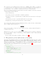
Basic structure of the input file
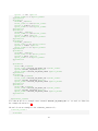
This is the basic structure of an input file:
<? xml version ="1.0"? >
<fit >
< macros >
...
</ macros >
< combined_model >
...
</ combined_model >
< chi_sqr_extra_term >
...
</ chi_sqr_extra_term >
< fit_settings >
...
</ fit_settings >
< parameter_values >
...
</ parameter_values >
< constant_values >
...
</ constant_values >
</ fit >
There has to be a root node, called fit, which contains (up to) five main nodes (in arbitrary order):
• macros [optional]: cf. section 5
5
• combined_model : cf. section 6
• chi_sqr_extra_term [optional] : cf. section 7
• fit_settings : cf. section 12
• parameter_values : cf. section 9
• constant_values [optional]: cf. section 9
5
The macros node
Here is an example:
< macros >
< macro >
< name > INITIAL_dE_START_VAL </ name >
< value > -1.1 </ value >
</ macro >
< macro >
< name > INITIAL_dE_PRIOR </ name >
< value > -1 </ value >
</ macro >
< macro >
< name > I NI TI AL_ dE _P RI OR_ WI DT H </ name >
< value > 1 </ value >
</ macro >
...
</ macros >
The macros node contains a list of macros, each of them with a unique name and a value. Both
are strings; spaces and newlines will be removed. For the example shown here, appearences of
INITIAL_dE_START_VAL in content nodes elsewhere in the XML document will be replaced by -1.1
etc.
6
The combined_models node
The combined_models node contains one or more individual models, to be fitted simultaneously.
Each individual model can either be a built-in model (cf. Sec. 13) or a completely user-defined model
(cf. Sec. 14).
An example for a combined_models node with 5 built-in models is shown below:
< combined_model >
< multi_alt_exp_expE_mat_model >
< n_exp > 8 < / n_exp >
< n_o_exp > 8 </ n_o_exp >
< A_name > Ai </ A_name >
< B_name > Bi </ B_name >
< E_name > Ei </ E_name >
< dE_name > dEi </ dE_name >
< t_name > t </ t_name >
< dim_1 > 2 </ dim_1 >
< dim_2 > 1 </ dim_2 >
<! - - B 2 - point fn -->
6
< fit_domain >
< variable_name > t </ variable_name >
< range >
<min > 2 </ min >
<max > 32 </ max >
</ range >
</ fit_domain >
< plot_domain >
< variable_name > t </ variable_name >
< plot_order > 1 </ plot_order >
< range >
<min > 0 </ min >
<max > 32 </ max >
</ range >
< step > 1 </ step >
</ plot_domain >
< data_file >
< file_type > ASCII </ file_type >
< file_name > r e _ B _ 2 x 1 _ m at r i x _ m o m _ 0 _ 0 _ 0 . dat </ file_name >
</ data_file >
</ multi_alt_exp_expE_mat_model >
< multi_alt_exp_Asqr_expE_BC_model > <! - - Kstar 2 - point fn -->
< n_exp > 8 </ n_exp >
< n_o_exp > 8 </ n_o_exp >
< A_name > Af </ A_name >
< B_name > Bf </ B_name >
< E_name > Ef </ E_name >
< dE_name > dEf </ dE_name >
< t_name > t </ t_name >
< T_name > L4 </ T_name >
< fit_domain >
< variable_name >t </ variable_name >
< range >
<min > 1 </ min >
<max > 20 </ max >
</ range >
< range >
<min > 44 </ min >
<max > 63 </ max >
</ range >
</ fit_domain >
< plot_domain >
< variable_name > t </ variable_name >
< plot_order > 1 </ plot_order >
< range >
<min > 0 </ min >
<max > 64 </ max >
</ range >
< step > 0.01 </ step >
</ plot_domain >
< data_file >
< file_type > ASCII </ file_type >
< file_name > re _v_l s_xyz _mom _0_0_ 0 . dat </ file_name >
</ data_file >
</ multi_alt_exp_Asqr_expE_BC_model >
< threept_multi_alt_exp_expE_model >
<! - - B to Kstar 3 - point fn -->
7
< n_exp_initial > 8 </ n_exp_initial >
< n_o_exp_initial > 8 </ n_o_exp_initial >
< n_exp_final > 8 </ n_exp_final >
< n_o_exp_final > 8 </ n_o_exp_final >
< A_name > A </ A_name >
< B_name > B </ B_name >
< E_initial_name > Ei </ E_initial_name >
< dE_initial_name > dEi </ dE_initial_name >
< E_final_name > Ef </ E_final_name >
< dE_final_name > dEf </ dE_final_name >
< t_name > t </ t_name >
< T_name > T </ T_name >
< fit_domain >
< variable_name > t </ variable_name >
< range >
<min > 1 </ min >
<max > T -2 </ max >
</ range >
</ fit_domain >
< fit_domain >
< variable_name > T </ variable_name >
< range >
<min > 14 </ min >
<max > 16 </ max >
</ range >
</ fit_domain >
< plot_domain >
< variable_name > t </ variable_name >
< plot_order > 2 </ plot_order >
< range >
<min > 1 </ min >
<max > T -2 </ max >
</ range >
< step > 1 </ step >
</ plot_domain >
< plot_domain >
< variable_name > T </ variable_name >
< plot_order > 1 </ plot_order >
< range >
<min > 14 </ min >
<max > 16 </ max >
</ range >
< step > 1 </ step >
</ plot_domain >
< data_file >
< file_type > binary </ file_type >
< file_name > i m _ g j _ s 0 j g 5 _ s l _ p f _ 0 _ 0 _ 0 _ p _ 0 _ 0 _ 0 . bin </ file_name >
</ data_file >
</ threept_multi_alt_exp_expE_model >
< multi_exp_Asqr_expE_BC_model >
< n_exp > 1 </ n_exp >
< A_name > KAf </ A_name >
< B_name > KBf </ B_name >
< E_name > KEf </ E_name >
< dE_name > KdEf </ dE_name >
< t_name > t </ t_name >
< T_name > L4 </ T_name >
<! - - K 2 - point fn -->
8
< fit_domain >
< variable_name > t </ variable_name >
< range >
<min > 10 </ min >
<max > 54 </ max >
</ range >
</ fit_domain >
< plot_domain >
< variable_name > t </ variable_name >
< plot_order > 1 </ plot_order >
< range >
<min > 0 </ min >
<max > 64 </ max >
</ range >
< step > 0.01 </ step >
</ plot_domain >
< data_file >
< file_type > ASCII </ file_type >
< file_name > re_ps_ls_mom_0_0_0 . dat </ file_name >
</ data_file >
</ multi_exp_Asqr_expE_BC_model >
< threept_multi_alt_exp_expE_model >
<! - - B to K 3 - point fn -->
< n_exp_initial > 1 </ n_exp_initial >
< n_o_exp_initial > 1 </ n_o_exp_initial >
< n_exp_final > 1 </ n_exp_final >
< n_o_exp_final > 0 </ n_o_exp_final >
< A_name > KA </ A_name >
< B_name > KB </ B_name >
< E_initial_name > Ei </ E_initial_name >
< dE_initial_name > dEi </ dE_initial_name >
< E_final_name > KEf </ E_final_name >
< dE_final_name > KdEf </ dE_final_name >
< t_name > t </ t_name >
< T_name > T </ T_name >
< fit_domain >
< variable_name > t </ variable_name >
< range >
<min > 6 </ min >
<max > T -12 </ max >
</ range >
</ fit_domain >
< fit_domain >
< variable_name > T </ variable_name >
< range >
<min > 0 </ min >
<max > 26 </ max >
</ range >
</ fit_domain >
< plot_domain >
< variable_name > t </ variable_name >
< plot_order > 2 </ plot_order >
< range >
<min > 0 </ min >
<max > T </ max >
</ range >
< step > 1 </ step >
</ plot_domain >
9
< plot_domain >
< variable_name > T </ variable_name >
< plot_order > 1 </ plot_order >
< range >
<min > 0 </ min >
<max > 26 </ max >
</ range >
< step > 1 </ step >
</ plot_domain >
< data_file >
< file_type > binary </ file_type >
< file_name > r e _ g 5 _ g 0 _ s l _ p f _ 0 _ 0 _ 0 _ p _ 0 _ 0 _ 0 . bin </ file_name >
</ data_file >
</ threept_multi_alt_exp_expE_model >
</ combined_model >
Every model has the nodes fit_domain (see Sec. 10 for more details), data_file, and plot_domain
(the latter is only needed when plotting). The allowed values for the property file_type are ASCII
and binary. For the other properties, see the descriptions of the individual models in Secs. 13 and
14. For the built-in models, he strings entered in fields such as dE_name are used as templates for the
parameter names. XMBF will “decorate” the names with additional indices as appropriate; see Sec. 13
for more details.
Fit parameters (and constants) with the same names will be shared between individual models, i.e.
they are forced to have the same value globally. Note that variable names are only used individually
for each model and only serve to specify the individual fitting ranges. It does not matter whether two
models have a common variable name or not.
7
The chi_sqr_extra_term node
The optional chi_sqr_extra_term node can be used to add an arbitrary function of the fit parameters
to χ2 . Note that it must be enabled separately by putting the line “<chi_sqr_extra_term_enabled>
true </chi_sqr_extra_term_enabled>” in the fit_settings node. Here is an example, which forces
two fit parameters a and b to have similar values within a width sigma_a_b, and puts a non-gaussian
constraint on another parameter c:
< chi_sqr_extra_term >
< function > sqr (a - b )/ sqr ( sigma_a_b ) + exp ( sqr (c -1.0)/ sqr ( sigma_c )) </ function >
< constant >
< name > sigma_a_b </ name >
< value > 0.1 </ value >
</ constant >
< constant >
< name > sigma_c </ name >
< value > 0.01 </ value >
</ constant >
< num_diff_step > 1e -8 </ num_diff_step >
</ chi_sqr_extra_term >
In general, the function can be constructed using the elementary operations
10
+, -, *, /,
(, ),
exp(...), log(...),
sin(...), cos(...), tan(...),
sinh(...), cosh(...), tanh(...),
arcsin(...), arccos(...), arctan(...),
sqr(...), sqrt(...),
alt(...).
The function may contain any of the fit parameters resulting from the models in combined_model. It
may also contain the constants defined inside chi_sqr_extra_term, as well as numerical literal values.
The derivatives of the function with respect to the fit parameters are calculated numerically using the
step size defined via num_diff_step.
8
The fit_settings node
< fit_settings >
< restrict_data_range > false </ restrict_data_range >
< data_range_min > 1 </ data_range_min >
< data_range_max > 1000 </ data_range_max >
< chi_sqr_extra_term_enabled > false </ chi_sqr_extra_term_enabled >
< bayesian > true </ bayesian >
< random_priors > true </ random_priors >
< num_diff_first_order > false </ num_diff_first_order >
< second_deriv_covariance > false </ second_deriv_covariance >
< second_deriv_minimization > false </ second_deriv_minimization >
< num_diff_step > 1e -08 </ num_diff_step >
< start_lambda > 0.001 </ start_lambda >
< lambda_factor > 10 </ lambda_factor >
< chi_sqr_tolerance > 0.001 </ chi_sqr_tolerance >
< chi_sqr_per_dof_tolerance > true </ chi_sqr_per_dof_tolerance >
< n_parameters_dof > 18 </ n_parameters_dof >
< inversion_method > LU </ inversion_method >
< bootstrap_normalization > false </ bootstrap_normalization >
< svd_fixed_cut > 0 </ svd_fixed_cut >
< svd_ratio_cut > 1e -06 </ svd_ratio_cut >
< svd_absolute_cut > 1e -06 </ svd_absolute_cut >
< max_iterations > 1000 </ max_iterations >
< bin_size > 1 </ bin_size >
< bootstrap_samples > 500 </ bootstrap_samples >
< use_bse_file > true </ use_bse_file >
< bse_file > b o o t s t r a p _ 1 6 0 0 c o n f i g s _ 5 0 0 s a m p l e s . bse </ bse_file >
< restrict_bootstrap_range > false </ restrict_bootstrap_range >
< bootstrap_range_min >1 </ bootstrap_range_min >
< bootstrap_range_max >50 </ bootstrap_range_max >
</ fit_settings >
Most of the settings are as in to QMBF; see the documentation of QMBF.
The property chi_sqr_per_dof_tolerance specifies whether the numerical value entered in
chi_sqr_tolerance (the abortion criterion for the Levenberg-Marquardt iteration) is used for the
total χ2 or for χ2 /dof.
11
The optional property n_parameters_dof is analoguous to QMBF’s setting “Number of parameters
to be subtracted from d.o.f”. If this property is not present in the XML file, the default values are: 0
(for Bayesian fits), or the total number of parameters in the fit (for non-Bayesian fits).
The property inversion_method specifies the method used in the calculation of the inverse of the data
correlation matrix. Allowed values are:
• LU (for full inversion)
• svd_fixed_cut (remove given number of smallest eigenvalues)
• svd_ratio_cut (remove eigenvalues that are smaller than some given fraction of the largest
eigenvalue)
• svd_absolute_cut (remove eigenvalues smaller than some given value)
• diagonal (keep only diagonal elements in data correlation matrix)
One very important setting is bootstrap_normalization. If set to false, the data correlation matrix
will be normalized with the usual factor of
1
,
N (N − 1)
where N is the number of data sets. If set to true, the data correlation matrix will instead be
normalized with the factor
1
.
N −1
This is needed to get the correct error estimates for fit parameters for the case that the original data
file was created using bootstrap over data sets (e.g. in the calculation of ratios of three-point and
two-point functions).
For more details on the setting concerning bootstrap, see Sec. 11.
9
The parameter_values and constant_values nodes
An excerpt of the parameter_values node from an example XML file is shown below. Note: entries
with parameter names that are not needed for the models are allowed and will be simply be ignored.
This is very convenient if for example changing the number of exponentials in a fit. Also note: the
tags prior and prior_width for each parameter are only needed for Bayesian fits, which are enabled
using <bayesian> true </bayesian> in the fit_settings node (see Sec. 12).
< parameter_values >
< parameter >
< name > Ei </ name >
< start_value > -0.66 </ start_value >
< prior > -0.6622 </ prior >
< prior_width > 0.04 </ prior_width >
</ parameter >
< parameter >
< name > Eio </ name >
< start_value > -0.33 </ start_value >
12
< prior > -0.3270 </ prior >
< prior_width > 0.3 </ prior_width >
</ parameter >
< parameter >
< name > Ai__1 </ name >
< start_value > 0.054 </ start_value >
< prior > 0.0544017 </ prior >
< prior_width > 0.007 </ prior_width >
</ parameter >
< parameter >
< name > Aio__1 </ name >
< start_value > 0.044 </ start_value >
< prior > 0.04416 </ prior >
< prior_width > 0.07 </ prior_width >
</ parameter >
< parameter >
< name > Ai__2 </ name >
< start_value > 0.18 </ start_value >
< prior > 0.179835 </ prior >
< prior_width > 0.03 </ prior_width >
</ parameter >
< parameter >
< name > Aio__2 </ name >
< start_value > 0.16 </ start_value >
< prior > 0.16123 </ prior >
< prior_width > 0.2 </ prior_width >
</ parameter >
...
< parameter >
< name > dEi_1 </ name >
< start_value > INITIAL_dE_START_VAL </ start_value >
< prior > INITIAL_dE_PRIOR </ prior >
< prior_width > I NI TI AL_ dE _P RIO R_ WI DT H </ prior_width >
</ parameter >
< parameter >
< name > dEi_2 </ name >
< start_value > INITIAL_dE_START_VAL </ start_value >
< prior > INITIAL_dE_PRIOR </ prior >
< prior_width > I NI TI AL_ dE _P RIO R_ WI DT H </ prior_width >
</ parameter >
< parameter >
< name > dEi_3 </ name >
< start_value > INITIAL_dE_START_VAL </ start_value >
< prior > INITIAL_dE_PRIOR </ prior >
< prior_width > I NI TI AL_ dE _P RIO R_ WI DT H </ prior_width >
</ parameter >
...
</ parameter_values >
Note that in the above example, macros named INITIAL_dE_START_VAL etc. are used, as defined in
the example shown in Sec. 5.
Shown below is an example for the constant_values node:
< constant_values >
< constant >
13
< name > L4 </ name >
< value > 64 </ value >
</ constant >
</ constant_values >
10
More details on fit ranges
Every model inside combined_models (see Sec. 6) must have one node called fit_domain for each
variable of that model.
Every fit_domain node can contain an arbitrary number of range nodes, where every range node
specifies a condition on the value of the variable (required: min, max – see Sec. 10.1; optional: step –
see Sec. 10.2). Every fit domain is the union (rather than the intersection) of the individual ranges.
That is, a fit point is included in the fit if and only if the value of every variable at that point satisfies
the condition of at least one of its range nodes.
10.1
Lower and upper bounds
Every range node must have two entries called min and max. These entries can contain numerical
values (integer or floating point), but also functions of other variables and constants (for example,
in the model threept_multi_alt_exp_expE_model shown in Sec. 6, the range for the variable t is
<min>1</min> and <max>T-2</max>, where T is the other variable. The function strings are parsed by
XMBF; the allowed operations are the same as given in Sec. 14. If no step (see Sec. 10.2) is specified
in the range node, a value x of a variable is considered inside the range if min ≤ x ≤ max.
10.2
Step sizes
Every range node can contain an optional entry called step, which must contain a step size ∆, which is
a positive numerical value (integer or floating point). In this case, a value x of a variable is considered
inside the range if in addition to statisfying min ≤ x ≤ max, the value satisfies as x = min + n · ∆,
where n is an integer.
11
11.1
More details on bootstrap
Resampling the data
When starting XMBF with the command-line option -b directory, the program performs the bootstrap procedure and writes the results for each parameter into an individual file in directory. The
output files have names that are combinations of the XML input file name and the parameter names.
On multi-core systems, the bootstrap procedure can be parallelized using XMBF_mpi instead of XMBF
(see Sec. 3.2).
The number of bootstrap samples is specified in the fit_settings node via bootstrap_samples.
Each bootstrap sample is obtained by randomly choosing N out of the N data configurations with
allowed repetitions. XMBF will recompute and invert the data correlation matrix for every single
bootstrap sample.
When the bootstrap is completed, the bootstrap averages and error estimates (based on sorting the
results and taking the 68% central part of the distributions) of the fit results are also printed to the
standard output.
14
By default, the random numbers of configurations are generated by XMBF at run time just before
the bootstrap. Alternatively, if the option use_bse_file in the fit_settings node is set to true, the
numbers are read from a text file, specified in bse_file. The format of a bootstrap ensemble file is as
follows: the number of bootstrap samples S, followed by the number of configurations N , followed by
S · N random integer numbers in the range 1...N . Such files can also be generated by QMBF (see the
QMBF manual).
For Bayesian fitting, it is recommended to set the option random_priors to true, in order to
get the (approximately) correct probability distribution. If this is activated, in addition to randomly
choosing data set ensembles, the priors will be choosen randomly from Gaussian distributions with the
given prior widths. This option does not affect the bootstrap for non-Bayesian fits.
Finally, by setting the optional property restrict_bootstrap_range to true, the bootstrap procedure can be restricted to a certain range of the samples, specified using bootstrap_range_min and
bootstrap_range_max. When a restricted range in the input XML file is specified, only only the
appropriate part of the .bse file will be used. Note that the option restrict_bootstrap_range is
fully compatible with random_priors: if bootstrap_range_min is greater than 1, the correct amount
of random numbers is skipped, so that also the sequence of random numbers for the priors remains
unchanged.
11.2
Resampling both the data and the fit ranges
XMBF can performed a generalized bootstrap procedure such that at the same time as resampling
the data configurations (and parameter priors, if activated), the fit ranges for the variables are also
resampled. This allows the incorporation of systematic errors due to the choices of the fitting ranges
into the bootstrap distribution.
Every range node can have an optional entry called range_bootstrap_file, which contains the
name of a file with the ranges for bootstrap (generated by the user). For example:
< fit_domain >
< variable_name > t </ variable_name >
< range >
<min > 8 </ min >
<max > T -12 </ max >
< range_bootstrap_file > BK3pt . brf </ range_bootstrap_file >
</ range >
</ fit_domain >
< fit_domain >
< variable_name >T </ variable_name >
< range >
<min > 0 </ min >
<max > 26 </ max >
</ range >
</ fit_domain >
In this case, the explicit range specified for the variable t via min and max (8 to T −12) are only used for
the initial fit when XMBF starts, but not for the bootstrap. During the bootstrap, the values for min
and max for each bootstrap sample are instead read from the file specified in range_bootstrap_file,
in this case “BK3pt.brf”. This number of lines in this file must be equal to bootstrap_samples, and
every line must have two entries, the min and max. As discussed in Sec. 10.1, these entries may also
contain functions of constants and other variables (but the functions must not contain whitespaces).
The first few lines of the file “BK3pt.brf” in the example could for example be
15
5
10
7
13
T -12
T -14
T -12
T -13
As discussed in Sec. 10.1, in XMBF every fit_domain can have multiple range nodes, and the actual
fit range is the union of the ranges. It is allowed that some range nodes do not have a range_bootstrap_file while others do.
An optional step value (Sec. 10.2) inside a range node is respected during the bootstrap even if a
range_bootstrap_file is used.
12
Multifit
When starting XMBF with the command-line option -m directory, the program performs the “multifit” procedure and writes the results for each parameter into an individual file in directory. The
output files have names that are combinations of the XML input file name and the parameter names.
The “multifit” procedure is the following: XMBF performs N successive fits, where the nth fit uses
just the nth data sample instead of the average over all data samples. The covariance matrix stays
fixed and is computed as usual using all data samples.
The “multifit” procedure is useful when the data samples themselves were obtained through a
bootstrap procedure, and a corresponding resampling of the fit results is wanted.
For Bayesian fitting, it is recommended to set the option random_priors in the fit_settings
node (see Sec. ) to true, in order to get the (approximately) correct probability distribution for the
fit parameters. If this is activated, the priors for each fit will be drawn randomly from Gaussian
distributions with the given prior widths and central values. This option does not affect the multifit
procedure for non-Bayesian fits.
13
Built-in Models
In the following, those parts of the parameter, constant, and variable names that are specified by the
user are typeset in typewriter font.
13.1
13.1.1
Scalar two-point models
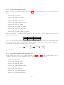
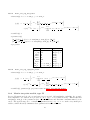
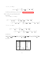
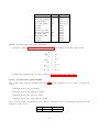
multi_exp_model
• function(s):
"
f (t) = A e−E
t
+
N
−1
X
n=1
• variable(s): t
• parameter(s): A, {B n}, E, {dE n}
• properties:
16
#
B n e−(E+dE 1+...+dE n)t
Key
n_exp
A_name
B_name
E_name
dE_name
t_name
13.1.2
content
N
A
B
E
dE
t
type
integer ≥ 1
string
string
string
string
string
multi_exp_expE_model
• function(s):
"
−eE t
f (t) = A e
+
N
−1
X
#
B ne
−(eE +edE 1 +...+edE n )t
n=1
• variable(s), parameter(s), properties: same as multi_exp_model
13.1.3
multi_exp_Asqr_model
• function(s):
"
2
f (t) = A
e
−E t
+
N
−1
X
#
2
(B n) e
−(E+dE 1+...+dE n)t
n=1
• variable(s), parameter(s), properties: same as multi_exp_model
13.1.4
multi_exp_Asqr_expE_model
• function(s):
"
f (t) = A2 e
−eE
t
+
N
−1
X
#
−(eE +edE 1 +...+edE n )t
(B n)2 e
n=1
• variable(s), parameter(s), properties: same as multi_exp_model
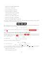
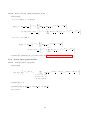
13.1.5
multi_alt_exp_model
• function(s):
"
−E t
f (t) = A e
+
N
−1
X
#
B ne
−(E+dE 1+...+dE n)t
n=1
"
+(−1)t+1 Ao e−Eo
t
+
M
−1
X
m=1
• variable(s): t
17
#
Bo m e−(Eo+dEo 1+...+dEo m)t
• parameter(s): A, {B n}, E, {dE n}, Ao, {Bo m}, Eo, {dEo m}
• properties:
Key
n_exp
n_o_exp
A_name
B_name
E_name
dE_name
t_name
13.1.6
content
N
M
A
B
E
dE
t
type
integer ≥ 1
integer ≥ 1
string
string
string
string
string
multi_alt_exp_expE_model
• function(s):
N
−1
X
"
f (t) = A e
−eE t
+
#
B ne
−(eE +edE 1 +...+edE n )t
n=1
"
−eEo
+(−1)t+1 Ao e
t
+
M
−1
X
#
Bo m e
−(eEo +edEo 1 +...+edEo m )t
m=1
• variable(s), parameter(s), properties: same as multi_alt_exp_model
13.1.7
multi_alt_exp_Asqr_model
• function(s):
"
2
f (t) = A
e
−E t
+
N
−1
X
#
−(E+dE 1+...+dE n)t
2
(B n) e
n=1
M
−1
X
"
+(−1)t+1 Ao 2 e−Eo
t
#
(Bo m)2 e−(Eo+dEo 1+...+dEo m)t
+
m=1
• variable(s), parameter(s), properties: same as multi_alt_exp_model
13.1.8
multi_alt_exp_Asqr_expE_model
• function(s):
"
−eE
f (t) = A2 e
t
+
N
−1
X
#
(B n)2 e
−(eE +edE 1 +...+edE n )t
n=1
"
t+1
+(−1)
Ao
2
−eEo t
e
+
M
−1
X
#
2
(Bo m) e
−(eEo +edEo 1 +...+edEo
m=1
• variable(s), parameter(s), properties: same as multi_alt_exp_model
18
m )t
13.2
Vector two-point models
All the “scalar” two-point models listed in section 13.1 are also available as “vector” two-point models,
called
• multi_exp_vec_model
• multi_exp_expE_vec_model
• multi_exp_Asqr_vec_model
• multi_exp_Asqr_expE_vec_model
• multi_alt_exp_vec_model
• multi_alt_exp_expE_vec_model
• multi_alt_exp_Asqr_vec_model
• multi_alt_exp_Asqr_expE_vec_model
These models require one further key in addition to the keys of the corresponding scalar models: the
dimension of the vector:
Key
dim
content
i = 1...dim
type
integer ≥ 1
A vector model has then dim functions fi (t) (i = 1...dim) of the same form as the underlying scalar
model. These functions have individual amplitude parameters, but share all the energy parameters.
For example, the functions for multi_exp_vec_model are
"
#
N
−1
X
−E t
−(E+dE 1+...+dE n)t
fi (t) = A i e
+
B n ie
n=1
for i = 1...dim.
13.3
Two-point models with periodic B.C.
All the “scalar” and “vector” two-point models listed in 13.1 and 13.2 are also available with periodic
boundary conditions. The models with periodic boundary conditions are called
• multi_exp_BC_model
• multi_exp_expE_BC_model
• multi_exp_Asqr_BC_model
• multi_exp_Asqr_expE_BC_model
• multi_alt_exp_BC_model
• multi_alt_exp_expE_BC_model
• multi_alt_exp_Asqr_BC_model
19
• multi_alt_exp_Asqr_expE_BC_model
• multi_exp_vec_BC_model
• multi_exp_expE_vec_BC_model
• multi_exp_Asqr_vec_BC_model
• multi_exp_Asqr_expE_vec_BC_model
• multi_alt_exp_vec_BC_model
• multi_alt_exp_expE_vec_BC_model
• multi_alt_exp_Asqr_vec_BC_model
• multi_alt_exp_Asqr_expE_vec_BC_model
and require one further key in addition to the keys of the underlying models: the name of the constant
corresponding to the temporal extent (of the lattice):
Key
T_name
content
T
type
string
The models with periodic boundary conditions have the same parameters as the underlying models.
The only difference is the replacement
→
fi (t)
fi (t) + fi (T − t)
for all functions fi of the model. The value of T has to be specified in the constant_values node; see
section 9.
13.4
Two-point models with time-independent contributions
For all the “scalar” and “vector” two-point models listed in 13.1 and 13.2, as well as their versions with
periodic boundary conditions (Sec. 13.3), an additional version exists, which adds time-independent
pieces to the fit function:
f (t) → f (t) + C
for scalar models,
f (t) + C + (−1)t+1 Co
→
f (t)
for scalar models with oscillating contributions,
fi (t)
→
fi (t) + C i
for vector models, and
fi (t)
→
fi (t) + C i + (−1)t+1 Co i
for vector models with oscillating contributions. The quantities C, Co, {C i}, {Co i} (as appropriate)
are additional fit parameters. These models are called
• multi_exp_const_model
• multi_exp_expE_const_model
20
• multi_exp_Asqr_const_model
• multi_exp_Asqr_expE_const_model
• multi_alt_exp_const_model
• multi_alt_exp_expE_const_model
• multi_alt_exp_Asqr_const_model
• multi_alt_exp_Asqr_expE_const_model
• multi_exp_vec_const_model
• multi_exp_expE_vec_const_model
• multi_exp_Asqr_vec_const_model
• multi_exp_Asqr_expE_vec_const_model
• multi_alt_exp_vec_const_model
• multi_alt_exp_expE_vec_const_model
• multi_alt_exp_Asqr_vec_const_model
• multi_alt_exp_Asqr_expE_vec_const_model
• multi_exp_BC_const_model
• multi_exp_expE_BC_const_model
• multi_exp_Asqr_BC_const_model
• multi_exp_Asqr_expE_BC_const_model
• multi_alt_exp_BC_const_model
• multi_alt_exp_expE_BC_const_model
• multi_alt_exp_Asqr_BC_const_model
• multi_alt_exp_Asqr_expE_BC_const_model
• multi_exp_vec_BC_const_model
• multi_exp_expE_vec_BC_const_model
• multi_exp_Asqr_vec_BC_const_model
• multi_exp_Asqr_expE_vec_BC_const_model
• multi_alt_exp_vec_BC_const_model
• multi_alt_exp_expE_vec_BC_const_model
• multi_alt_exp_Asqr_vec_BC_const_model
21
• multi_alt_exp_Asqr_expE_vec_BC_const_model
and require one further key in addition to the keys of the underlying models: the name template for
the new parameter(s):
Key
C_name
13.5
content
C
type
string
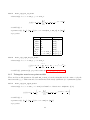
Matrix two-point models
Matrix models are very different from vector models. In matrix models, it is assumed that the amplitudes factor into an outer product of a vector with itself, like A i A j, where the A i are used as fit
parameters.
In the following, the functions are labelled by two indices i, j. The required storage order in the
data files is such that the first index (i) runs slow and the second index (j) runs fast.
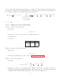
13.5.1
multi_exp_mat_model
• function(s): for i = 1...dim_1, j = 1...dim_2:
"
fij (t) = A i A j
e
−E t
+
N
−1
X
#
−(E+dE 1+...+dE n)t
Bn i Bn j e
n=1
• variable(s): t
• parameter(s): {A i}, {B n i} (for i = 1...max(dim_1, dim_2)), E, {dE n}
• properties:
Key
n_exp
A_name
B_name
E_name
dE_name
t_name
dim_1
dim_2
13.5.2
content
N
A
B
E
dE
t
i = 1...dim_1
j = 1...dim_2
type
integer ≥ 1
string
string
string
string
string
integer ≥ 1
integer ≥ 1
multi_exp_expE_mat_model
• function(s): for i = 1...dim_1, j = 1...dim_2:
"
fij (t) = A i A j
−eE
e
t
+
N
−1
X
#
−(eE +edE 1 +...+edE n )t
Bn i Bn j e
n=1
• variable(s), parameter(s), properties: same as multi_exp_mat_model
22
13.5.3
multi_alt_exp_mat_model
• function(s): for i = 1...dim_1, j = 1...dim_2:
"
e−E
fij (t) = A i A j
t
+
N
−1
X
#
B n i B n j e−(E+dE 1+...+dE n)t
n=1
"
t+1
+(−1)
Ao i Ao j
e
−Eo t
+
M
−1
X
#
−(Eo+dEo 1+...+dEo m)t
Bo m i Bo m j e
m=1
• variable(s): t
• parameter(s):
{A i}, {B n i} (for i = 1...max(dim_1, dim_2)), E, {dE n},
{Ao i}, {Bo m i} (for i = 1...max(dim_1, dim_2)), Eo, {dEo m},
• properties:
Key
n_exp
n_o_exp
A_name
B_name
E_name
dE_name
t_name
dim_1
dim_2
13.5.4
content
N
M
A
B
E
dE
t
i = 1...dim_1
j = 1...dim_2
type
integer
integer
string
string
string
string
string
integer
integer
≥1
≥1
≥1
≥1
multi_alt_exp_expE_mat_model
• function(s): for i = 1...dim_1, j = 1...dim_2:
"
fij (t) = A i A j
e
−eE
t
+
N
−1
X
#
−(eE +edE 1 +...+edE n )t
Bn i Bn j e
n=1
"
+(−1)t+1 Ao i Ao j
e
−eEo t
+
M
−1
X
#
−(eEo +edEo 1 +...+edEo m )t
Bo m i Bo m j e
m=1
• variable(s), parameter(s), properties: same as multi_alt_exp_mat_model
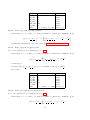
13.6
Matrix two-point models, type II
In type II matrix models, the ground state is not special. All amplitudes, including the groundstate amplitude, are written as a product A i B n i (i.e., n now starts from 0). This means that
max(dim_1, dim_2) of the parameters {B n i} are redundant, and Bayesian constraints must be activated. The typical usage is to constrain the parameters B (i − 1) i to 1 ± with a very small prior
width , which effectively eliminates these parameters from the functions.
23
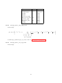
13.6.1
multi_exp_mat_II_model
• function(s): for i = 1...dim_1, j = 1...dim_2:
fij (t) = A i A j
N
−1
X
B n i B n j e−(E+...+dE n)t
n=0
• variable(s): t
• parameter(s): {A i}, {B n i} (for i = 1...max(dim_1, dim_2)), E, {dE n}
• properties:
Key
n_exp
A_name
B_name
E_name
dE_name
t_name
dim_1
dim_2
13.6.2
content
N
A
B
E
dE
t
i = 1...dim_1
j = 1...dim_2
type
integer ≥ 1
string
string
string
string
string
integer ≥ 1
integer ≥ 1
multi_exp_expE_mat_II_model
• function(s): for i = 1...dim_1, j = 1...dim_2:
fij (t) = A i A j
N
−1
X
E +...+edE n )t
B n i B n j e−(e
n=0
• variable(s), parameter(s), properties: same as multi_exp_mat_II_model
13.7
Triangular matrix two-point models
These models are like matrix models with dim_1=dim_2, but the triangular models consist of only the
functions with j ≥ i. This is intended for matrix fits with exactly symmetric (i.e. symmetrized) data.
13.7.1
multi_exp_mat_upper_model
• function(s): for i = 1...dim, j = i...dim (total number of functions = dim(dim + 1)/2):
"
fij (t) = A i A j
e
−E t
+
N
−1
X
#
Bn i Bn j e
n=1
• variable(s): t
• parameter(s): {A i}, {B n i} (for i = 1...dim), E, {dE n}
• properties:
24
−(E+dE 1+...+dE n)t
Key
n_exp
A_name
B_name
E_name
dE_name
t_name
dim
13.7.2
content
N
A
B
E
dE
t
i = 1...dim, j = i...dim
type
integer ≥ 1
string
string
string
string
string
integer ≥ 1
multi_exp_expE_mat_upper_model
• function(s): for i = 1...dim, j = i...dim (total number of functions = dim(dim + 1)/2):
"
fij (t) = A i A j
−eE
e
t
+
N
−1
X
#
−(eE +edE 1 +...+edE n )t
Bn i Bn j e
n=1
• variable(s), parameter(s), properties: same as multi_exp_mat_upper_model
13.7.3
multi_exp_mat_II_upper_model
Note: some parameters are redundant (see Sec. 13.6).
• function(s): for i = 1...dim, j = i...dim (total number of functions = dim(dim + 1)/2):
fij (t) = A i A j
N
−1
X
B n i B n j e−(E+...+dE n)t
n=0
• variable(s): t
• parameter(s): {A i}, {B n i} (for i = 1...max(dim_1, dim_2)), E, {dE n}
• properties:
Key
n_exp
A_name
B_name
E_name
dE_name
t_name
dim
13.7.4
content
N
A
B
E
dE
t
i = 1...dim, j = i...dim
type
integer ≥ 1
string
string
string
string
string
integer ≥ 1
multi_exp_expE_mat_II_upper_model
Note: some parameters are redundant (see Sec. 13.6).
• function(s): for i = 1...dim, j = i...dim (total number of functions = dim(dim + 1)/2):
fij (t) = A i A j
N
−1
X
E +...+edE n )t
B n i B n j e−(e
n=0
25
• variable(s), parameter(s), properties: same as multi_exp_mat_II_upper_model
13.8
Non-symmetric matrix two-point models
Here the amplitudes are factorized into an outer product of two different vectors, rather than the outer
product of a vector with itself, as in the models of Sec. 13.5. Because of a reparametrization invariance,
some amplitude parameters need to be eliminated to get unique results. This has already been done
in the following models, so that the fit functions are different for i = 1 vs i > 1 (see below).
As in Sec. 13.5, the required storage order in the data files is such that the first index (i) runs slow
and the second index (j) runs fast.
13.8.1
multi_exp_nonsym_mat_model
• function(s):
for i = 2...dim_1, j = 1...dim_2:
"
fij (t) = Ax i Ay j
e
−E t
+
N
−1
X
#
−(E+dE 1+...+dE n)t
Bx n i By n j e
n=1
for i = 1, j = 1...dim_2:
"
f1j (t) = Ay j
e
−E t
+
N
−1
X
#
−(E+dE 1+...+dE n)t
By n j e
n=1
• variable(s): t
• parameter(s): {Ax i, Bx n i} (for i = 2...dim_1), {Ay j, By n j} (for j = 1...dim_2), E, {dE n}
• properties:
Key
n_exp
A_name
B_name
E_name
dE_name
t_name
dim_1
dim_2
13.8.2
content
N
A
B
E
dE
t
i = 1...dim_1
j = 1...dim_2
type
integer ≥ 1
string
string
string
string
string
integer ≥ 2
integer ≥ 1
multi_exp_expE_nonsym_mat_model
• function(s):
for i = 2...dim_1, j = 1...dim_2:
"
fij (t) = Ax i Ay j
−eE t
e
+
N
−1
X
n=1
26
#
−(eE +edE 1 +...+edE n )t
Bx n i By n j e
for i = 1, j = 1...dim_2:
"
f1j (t) = Ay j
−eE
e
t
+
N
−1
X
#
−(eE +edE 1 +...+edE n )t
By n j e
n=1
• variable(s), parameter(s), properties: same as multi_exp_nonsym_mat_model
13.8.3
multi_alt_exp_nonsym_mat_model
• function(s):
for i = 2...dim_1, j = 1...dim_2:
"
fij (t) = Ax i Ay j
e−E
t
+
N
−1
X
#
Bx n i By n j e−(E+dE 1+...+dE n)t
n=1
"
t+1
+(−1)
Aox i Aoy j
e
−Eo t
+
M
−1
X
#
−(Eo+dEo 1+...+dEo m)t
Box m i Boy m j e
m=1
for i = 1, j = 1...dim_2:
"
f1j (t) = Ay j
−E t
e
+
N
−1
X
#
−(E+dE 1+...+dE n)t
By n j e
n=1
"
+(−1)t+1 Aoy j
e−Eo
t
+
M
−1
X
#
Boy m j e−(Eo+dEo 1+...+dEo m)t
m=1
• variable(s): t
• parameter(s): {Ax i, Bx n i} (for i = 2...dim_1), {Ay j, By n j} (for j = 1...dim_2), E, {dE n},
{Aox i, Box m i} (for i = 2...dim_1), {Aoy j, Boy m j} (for j = 1...dim_2), Eo, {dEo n}
• properties:
Key
n_exp
n_o_exp
A_name
B_name
E_name
dE_name
t_name
dim_1
dim_2
content
N
M
A
B
E
dE
t
i = 1...dim_1
j = 1...dim_2
27
type
integer
integer
string
string
string
string
string
integer
integer
≥1
≥1
≥2
≥1
13.8.4
multi_alt_exp_expE_nonsym_mat_model
• function(s):
for i = 2...dim_1, j = 1...dim_2:
"
fij (t) = Ax i Ay j
e
−eE t
+
N
−1
X
#
−(eE +edE 1 +...+edE n )t
Bx n i By n j e
n=1
"
−eEo
+(−1)t+1 Aox i Aoy j
e
t
+
M
−1
X
#
−(eEo +edEo 1 +...+edEo m )t
Box m i Boy m j e
m=1
for i = 1, j = 1...dim_2:
"
f1j (t) = Ay j
e
−eE
t
+
N
−1
X
#
−(eE +edE 1 +...+edE n )t
By n j e
n=1
"
t+1
+(−1)
e
Aoy j
−eEo t
+
M
−1
X
#
−(eEo +edEo 1 +...+edEo
Boy m j e
m )t
m=1
• variable(s), parameter(s), properties: same as multi_alt_exp_nonsym_mat_model
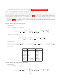
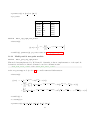
13.9
13.9.1
Scalar three-point models
threept_multi_exp_model
• function(s):
"
#
f (t, T) = A e−F t e−E(T−t) +
X
B n0 n e−(F+dF 1+...+dF
n = 0 ... N − 1,
n0 = 0 ... N 0 − 1,
(n, n0 ) 6= (0, 0)
• variable(s): t, T
• parameter(s): A, {B n0 n},
E, {dE n},
F, {dF n0 }
• properties:
28
n0 )t
e−(E+dE 1+...+dE n)(T−t)
Key
n_exp_initial
n_exp_final
A_name
B_name
E_initial_name
dE_initial_name
E_final_name
dE_final_name
t_name
T_name
13.9.2
content
N
N0
A
B
E
dE
F
dF
t
T
type
integer ≥ 1
integer ≥ 1
string
string
string
string
string
string
string
string
threept_multi_exp_expE_model
• function(s):
"
f (t, T) = A e
−eF t −eE (T−t)
e
X
+
0
−(eF +edF 1 +...+edF
Bn n e
n0 )t
#
e
−(eE +edE 1 +...+edE n )(T−t)
n = 0 ... N − 1,
n0 = 0 ... N 0 − 1,
(n, n0 ) 6= (0, 0)
• variable(s), parameter(s), properties: same as threept_multi_exp_model
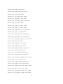
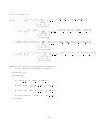
13.9.3
threept_multi_alt_exp_model
• function(s):
29
For M > 0 and M 0 > 0:
"
f (t, T)
=
#
X
Aee e−F t e−E(T−t) +
Bee n0 n e−(F+dF 1+...+dF
n0 )t
e−(E+dE 1+...+dE n)(T−t)
n = 0 ... N − 1,
n0 = 0 ... N 0 − 1,
(n, n0 ) 6= (0, 0)
"
+
(−1)t
#
−Fo t −E(T−t)
Aoe e
e
+
X
0
Boe m n e
−(Fo+dFo 1+...+dFo m0 )t
−(E+dE 1+...+dE n)(T−t)
e
n = 0 ... N − 1,
m0 = 0 ... M 0 − 1,
(n, m0 ) 6= (0, 0)
"
+
(−1)(T −t)
#
−F t −Eo(T−t)
Aeo e
e
+
X
0
Beo n m e
−(F+dF 1+...+dF n0 )t
−(Eo+dEo 1+...+dEo m)(T−t)
e
m = 0 ... M − 1,
n0 = 0 ... N 0 − 1,
(m, n0 ) 6= (0, 0)
#
"
+
(−1)T
−Fo t −Eo(T−t)
Aoo e
e
X
+
0
Boo m m e
m = 0 ... M − 1,
m0 = 0 ... M 0 − 1,
(m, m0 ) 6= (0, 0)
Note: for M 0 = 0, the second and fourth row disappear.
for M = 0, the third and fourth row disappear.
• variable(s): t, T
• parameter(s):
Aee, {Bee n0 n},
E, {dE n},
F, {dF n0 }
For M > 0 also
Aeo, {Beo n0 m},
For M 0 > 0 also
Aoe, {Boe m0 n},
For (M > 0 and M 0 > 0) also
Eo, {dEo m}
Fo, {dFo m0 }
Aoo, {Boo m0 m}
• properties:
30
−(Fo+dFo 1+...+dFo m0 )t
e
−(Eo+dEo 1+...+dEo m)(T−t)
Key
n_exp_initial
n_o_exp_initial
n_exp_final
n_o_exp_final
A_name
B_name
E_initial_name
dE_initial_name
E_final_name
dE_final_name
t_name
T_name
13.9.4
content
N
M
N0
M0
A
B
E
dE
F
dF
t
T
type
integer
integer
integer
integer
string
string
string
string
string
string
string
string
≥1
≥0
≥1
≥0
threept_multi_alt_exp_expE_model
• function: same as threept_multi_alt_exp_model, but with the following replacements:
E → eE
dE_n → edE_n
F → eF
dF_n0 → edF_n
0
Eo → eEo
dEo_m → edEo_m
Fo → eFo
0
dFo_m0 → edFo_m
• variable(s), parameter(s), properties: same as threept_multi_alt_exp_model
13.10
Vector three-point models
The “scalar” three-point models listed in section 13.9 are also available as “vector” three-point models,
called
• threept_multi_exp_vec_model
• threept_multi_exp_expE_vec_model
• threept_multi_alt_exp_vec_model
• threept_multi_alt_exp_expE_vec_model
These models require one further key in addition to the keys of the corresponding scalar models: the
dimension of the vector:
Key
dim
content
i = 1...dim
31
type
integer ≥ 1
A vector model has then dim functions fi (t) (i = 1...dim) of the same form as the underlying scalar
model. These functions have individual amplitude parameters, but share all the energy parameters.
For example, the functions for threept_multi_exp_vec_model are
"
#
X
−F t −E(T−t)
0
−(F+dF 1+...+dF n0 )t −(E+dE 1+...+dE n)(T−t)
fi (t, T) = A i e
e
+
Bn n i e
e
n = 0 ... N − 1,
n0 = 0 ... N 0 − 1,
(n, n0 ) 6= (0, 0)
for i = 1...dim.
13.11
13.11.1
“Degenerate” three-point models
threept_constant_model
• function(s):
f (t, T) = C
• variable(s): t, T (note: both t and T are a dummy variables.)
• parameter(s): C
• properties:
Key
C_name
t_name
T_name
13.11.2
content
C
t
T
type
string
string
string
threept_constant_sqr_model
• function(s):
f (t, T) = C2
• variable(s), parameter(s), properties: same as threept_constant_model
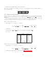
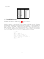
13.11.3
multi_exp_2var_model
• function(s):
"
f (t, T) = A e−E
T
+
N
−1
X
#
B n e−(E+dE 1+...+dE n)T
n=1
• variable(s): t, T (note: t is a dummy variable. This model is intended for fitting of three-point
functions in which the initial and the final state have identical energy levels, and the off-diagonal
transition matrix elements vanish. In this case, the t-dependence disappears.)
32
• parameter(s): A, {B n}, E, {dE n}
• properties:
Key
n_exp
A_name
B_name
E_name
dE_name
t_name
T_name
13.11.4
content
N
A
B
E
dE
t
T
type
integer ≥ 1
string
string
string
string
string
string
multi_exp_expE_2var_model
• function(s):
N
−1
X
"
−eE T
f (t, T) = A e
+
#
B ne
−(eE +edE 1 +...+edE n )T
n=1
• variable(s), parameter(s), properties: same as multi_exp_2var_model
13.12
13.12.1
Multi-particle two-point models
multi_part_exp_expE_model
This model was implemented by W. Detmold. Currently, it has no implementation of the symbolic
derivatives, and therefore this model must be used in combination with
< num_diff_first_order > true </ num_diff_first_order >
in the fit_settings node (see Sec. 12) to enable numerical differentiation.
• function(s):
E P (T/2)
f (t, T) = Z P e−e
bP/2c
+
X
p=1
+
N
−1
X
2
P
p
cosh(eE P (t − T/2))
E (P −p) +eE p )(T/2)
Z P A P p e−(e
E P +edE P 1 +...+edE P n )(T/2)
Z P B P n e−(e
n=1
• variable(s): t
• constant(s): T
• parameter(s): Z P , {A P p}, {B P n}, {E p}, {dE n}
33
cosh (eE (P −p) + eE p )(t − T/2)
cosh (eE P + edE P
1
+ ... + edE P n )(t − T/2)
• properties:
Key
n_exp
n_part
A_name
B_name
Z_name
E_name
dE_name
t_name
T_name
14
content
N
P
A
B
Z
E
dE
t
T
type
integer ≥ 1
integer ≥ 1
string
string
string
string
string
string
string
User-defined model
In addition to the built-in models listed in Sec. 13, there is a model called
parse_model,
which allows the user to completely define new models using only the XML input file. When using
parse_model, the functions (and, if necessary their first-order derivatives) are entered as strings and
parsed by XMBF. A parse_model of XMBF offers the same functionality as a user-defined model of
QMBF, allowing the definition of models with an arbitrary number of functions, variables, parameters, and constants. The functions (and derivatives) can be constructed using the same elementary
operations as in QMBF (the reader is referred to the QMBF manual for the details):
+, -, *, /,
(, ),
exp(...), log(...),
sin(...), cos(...), tan(...),
sinh(...), cosh(...), tanh(...),
arcsin(...), arccos(...), arctan(...),
sqr(...), sqrt(...),
alt(...).
34
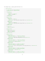
An example usage of parse_model is shown below:
< parse_model >
< n_variables > 1 </ n_variables >
< n_functions > 2 </ n_functions >
< variables >
< variable >
< number > 1 </ number >
< name > t </ name >
</ variable >
</ variables >
< functions >
< function >
< number > 1 </ number >
< definition > A_1 *( exp ( - E * t )+ exp ( - E *( T - t ))) </ definition >
</ function >
< function >
< number > 2 </ number >
< definition > A_2 *( exp ( - E * t )+ exp ( - E *( T - t ))) </ definition >
</ function >
</ functions >
< constants >
< name > T </ name >
</ constants >
< parameters >
< name > A_2 </ name >
< name > E </ name >
< name > A_1 </ name >
</ parameters >
< derivatives >
< derivative >
< function_number > 1 </ function_number >
< parameter_name > A_1 </ parameter_name >
< definition > exp ( - E * t )+ exp ( - E *( T - t )) </ definition >
</ derivative >
< derivative >
< function_number > 1 </ function_number >
< parameter_name > A_2 </ parameter_name >
< definition > 0 </ definition >
</ derivative >
< derivative >
< function_number > 1 </ function_number >
< parameter_name > E </ parameter_name >
< definition > A_1 *(( - t )* exp ( - E * t ) -(T - t )* exp ( - E *( T - t ))) </ definition >
</ derivative >
< derivative >
< function_number > 2 </ function_number >
< parameter_name > A_1 </ parameter_name >
< definition > 0 </ definition >
</ derivative >
< derivative >
< function_number > 2 </ function_number >
< parameter_name > A_2 </ parameter_name >
35
< definition > exp ( - E * t )+ exp ( - E *( T - t )) </ definition >
</ derivative >
< derivative >
< function_number > 2 </ function_number >
< parameter_name > E </ parameter_name >
< definition > A_2 *(( - t )* exp ( - E * t ) -(T - t )* exp ( - E *( T - t ))) </ definition >
</ derivative >
</ derivatives >
< fit_domain >
< variable_name > t </ variable_name >
< range >
<min > 10 </ min >
<max > 54 </ max >
</ range >
</ fit_domain >
< data_file >
< file_type > ASCII </ file_type >
< file_name > correlator . dat </ file_name >
</ data_file >
</ parse_model >
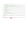
(this particular example actually reimplements the case of multi_exp_vec_BC_model with n_exp=1
and dim=2).
Note that the derivatives node in parse_model is only required if the option num_diff_first_order
in the fit_settings node (see Sec. 12) is set to false.
36