Download User`s manual

The fastcluster package: User’s manual
Version 1.1.9
Daniel Müllner
March 15, 2013
The fastcluster package is a C++ library for hierarchical, agglomerative clustering.
It efficiently implements the seven most widely used clustering schemes: single, complete, average, weighted/mcquitty, Ward, centroid and median linkage. The library
currently has interfaces to two languages: R and Python/SciPy. Part of the functionality is designed as drop-in replacement for existing routines: linkage in the SciPy
package scipy.cluster.hierarchy, hclust in R’s stats package, and the flashClust
package. Once the fastcluster library is loaded at the beginning of the code, every program that uses hierarchical clustering can benefit immediately and effortlessly from
the performance gain. Moreover, there are memory-saving routines for clustering of
vector data, which go beyond what the existing packages provide.
This document describes the usage for the two interfaces for R and Python and is meant
as the reference document for the end user. Installation instructions are given in the file
INSTALL in the source distribution and are not repeated here. The sections about the
two interfaces are independent and in consequence somewhat redundant, so that users who
need a reference for one interface need to consult only one section.
If you use the fastcluster package for scientific work, please cite it as:
Daniel Müllner, fastcluster: Fast hierarchical clustering routines for R and
Python, Version 1.1.9, 2012. Available at CRAN http://cran.r-project.org
and and PyPI http://pypi.python.org/pypi/fastcluster.
Contents
1 The R interface
hclust . . . . . . . . . . . . . . . . . . . . . . . . . . . . . . . . . . . . . . . . . .
hclust.vector . . . . . . . . . . . . . . . . . . . . . . . . . . . . . . . . . . . . .
1
2
3
5
2 The Python interface
linkage . . . . . . . .
single . . . . . . . . .
complete . . . . . . .
average . . . . . . . .
weighted . . . . . . .
centroid . . . . . . .
median . . . . . . . . .
ward . . . . . . . . . .
linkage_vector . . .
.
.
.
.
.
.
.
.
.
.
.
.
.
.
.
.
.
.
.
.
.
.
.
.
.
.
.
.
.
.
.
.
.
.
.
.
.
.
.
.
.
.
.
.
.
.
.
.
.
.
.
.
.
.
.
.
.
.
.
.
.
.
.
.
.
.
.
.
.
.
.
.
.
.
.
.
.
.
.
.
.
.
.
.
.
.
.
.
.
.
.
.
.
.
.
.
.
.
.
.
.
.
.
.
.
.
.
.
.
.
.
.
.
.
.
.
.
.
.
.
.
.
.
.
.
.
.
.
.
.
.
.
.
.
.
.
.
.
.
.
.
.
.
.
.
.
.
.
.
.
.
.
.
.
.
.
.
.
.
.
.
.
.
.
.
.
.
.
.
.
.
.
.
.
.
.
.
.
.
.
.
.
.
.
.
.
.
.
.
.
.
.
.
.
.
.
.
.
.
.
.
.
.
.
.
.
.
.
.
.
.
.
.
.
.
.
.
.
.
.
.
.
.
.
.
.
.
.
.
.
.
.
.
.
.
.
.
.
.
.
.
.
.
.
.
.
.
.
.
.
.
.
.
.
.
.
.
.
.
.
.
.
.
.
.
.
.
.
.
.
.
.
.
.
.
.
.
.
.
.
.
.
.
.
.
.
.
.
.
.
.
.
.
.
.
.
.
6
7
10
10
10
10
10
10
10
10
3 Behavior for NaN and infinite values
14
4 Differences between the two interfaces
15
5 References
15
1 The R interface
Load the package with the following command:
library('fastcluster')
The package overwrites the function hclust from the stats package (in the same way as
the flashClust package does). Please remove any references to the flashClust package in
your R files to not accidentally overwrite the hclust function with the flashClust version.
The new hclust function has exactly the same calling conventions as the old one. You
may just load the package and immediately and effortlessly enjoy the performance improvements. The function is also an improvement to the flashClust function from the
flashClust package. Just replace every call to flashClust by hclust and expect your
code to work as before, only faster.1 In case the data includes infinite or NaN values, see
Section 3.
If you need to access the old function or make sure that the right function is called,
specify the package as follows:
fastcluster::hclust(...)
flashClust::hclust(...)
stats::hclust(...)
Vector data can be clustered with a memory-saving algorithm with the command:
1 If
you are using flashClust prior to version 1.01, update it! See the change log for flashClust at
http://cran.r-project.org/web/packages/flashClust/ChangeLog.
2
hclust.vector(...)
The following sections contain comprehensive descriptions of these methods.
hclust (d, method='complete', members=NULL)
Hierarchical, agglomerative clustering on a condensed dissimilarity matrix.
This method has the same specifications as the method hclust in the package stats
and hclust alias flashClust in the package flashClust. In particular, the print,
plot, rect.hclust and identify methods work as expected.
The argument d is a condensed distance matrix, as it is produced by dist.
The argument method is one of the strings 'single', 'complete', 'average', 'mcquitty',
'centroid', 'median', 'ward', or an unambiguous abbreviation thereof.
The argument members specifies the sizes of the initial nodes, ie. the number of
observations in the initial clusters. The default value NULL says that all initial nodes
are singletons, ie. have size 1. Otherwise, members must be a vector whose size is the
number of input points. The vector is processed as a double array so that not only
integer cardinalities of nodes can be accounted for but also weighted nodes with real
weights.
The general scheme of the agglomerative clustering procedure is as follows:
1. Start with N singleton clusters (nodes) labeled −1, . . . , −N , which represent the
input points.
2. Find a pair of nodes with minimal distance among all pairwise distances.
3. Join the two nodes into a new node and remove the two old nodes. The new
nodes are labeled consecutively 1, 2, . . .
4. The distances from the new node to all other nodes is determined by the method
parameter (see below).
5. Repeat N − 1 times from step 2, until there is one big node, which contains all
original input points.
The output of hclust is an object of class 'hclust' and represents a stepwise dendrogram. It contains the following fields:
merge This is an (N − 1) × 2 array. Row i specifies the labels of the nodes which are
joined step i of the clustering.
height This is a vector of length N − 1. It contains the sequence of dissimilarities at
which every pair of nearest nodes is joined.
order This is a vector of length N . It contains a permutation of the numbers 1, . . . N
for the plot method. When the dendrogram is plotted, this is the order in
which the singleton nodes are plotted as the leaves of a rooted tree. The order
is computed so that the dendrogram is plotted without intersections (except the
3
case when there are inversions for the 'centroid' and 'median' methods). The
choice of the 'order' sequence follows the same scheme as the stats package does,
only with a faster algorithm. Note that there are many valid choices to order
the nodes in a dendrogram without intersections. Also, subsequent points in the
'order' field are not always close in the ultrametric given by the dendrogram.
labels This copies the attribute 'Labels' from the first input parameter d. It contains
the labels for the objects being clustered.
method The (unabbreviated) string for the 'method' parameter. See below for a
specification of all available methods.
call The full command that produced the result. See match.call.
dist.method This 'method' attribute of the first input parameter d. This specifies
which metric was used in the dist method which generated the first argument.
The parameter method specifies which clustering scheme to use. The clustering scheme
determines the distance from a new node to the other nodes. Denote the dissimilarities
by d, the nodes to be joined by I, J, the new node by K and any other node by L.
The symbol |I| denotes the size of the cluster I.
method='single': d(K, L) = min(d(I, L), d(J, L))
The distance between two clusters A, B is the closest distance between any two
points in each cluster:
d(A, B) = min d(a, b)
a∈A,b∈B
method='complete': d(K, L) = max(d(I, L), d(J, L))
The distance between two clusters A, B is the maximal distance between any
two points in each cluster:
d(A, B) =
max d(a, b)
a∈A,b∈B
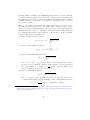
|I| · d(I, L) + |J| · d(J, L)
|I| + |J|
The distance between two clusters A, B is the average distance between the
points in the two clusters:
method='average': d(K, L) =
d(A, B) =
1
|A||B|
∑
d(a, b)
a∈A,b∈B
method='mcquitty': d(K, L) = 12 (d(I, L) + d(J, L))
There is no global description for the distance between clusters since the distance
depends on the order of the merging steps.
4
The following three methods are intended for Euclidean data only, ie. when X contains
the pairwise squared distances between vectors in Euclidean space. The algorithm
will work on any input, however, and it is up to the user to make sure that applying
the methods makes sense.
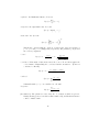
|I| · d(I, L) + |J| · d(J, L) |I| · |J| · d(I, J)
method='centroid': d(K, L) =
−
|I| + |J|
(|I| + |J|)2
There is a geometric interpretation: d(A, B) is the distance between the centroids
(ie. barycenters) of the clusters in Euclidean space:
d(A, B) = ∥⃗cA − ⃗cB ∥2 ,
where ⃗cA denotes the centroid of the points in cluster A.
method='median': d(K, L) = 21 d(I, L) + 12 d(J, L) − 14 d(I, J)
Define the midpoint w
⃗ K of a cluster K iteratively as w
⃗ K = k if K = {k} is a
⃗I + w
⃗ J ) if K is formed by joining I and J.
singleton and as the midpoint 21 (w
Then we have
d(A, B) = ∥w
⃗A − w
⃗ B ∥2
in Euclidean space for all nodes A, B. Notice however that this distance depends
on the order of the merging steps.
(|I| + |L|) · d(I, L) + (|J| + |L|) · d(J, L) − |L| · d(I, J)
method='ward': d(K, L) =
|I| + |J| + |L|
The global cluster dissimilarity can be expressed as
d(A, B) =
2|A||B|
· ∥⃗cA − ⃗cB ∥2 ,
|A| + |B|
where ⃗cA again denotes the centroid of the points in cluster A.
hclust.vector (X, method='single', members=NULL, metric='euclidean', p=NULL)
This performs hierarchical, agglomerative clustering on vector data with memorysaving algorithms. While the hclust method requires Θ(N 2 ) memory for clustering
of N points, this method needs Θ(N D) for N points in RD , which is usually much
smaller.
The argument X must be a two-dimensional matrix with double precision values. It
describes N data points in RD as an (N × D) matrix.
The parameter 'members' is the same as for hclust.
The parameter 'method' is one of the strings 'single', 'centroid', 'median', 'ward', or
an unambiguous abbreviation thereof.
If method is 'single', single linkage clustering is performed on the data points with
the metric which is specified by the metric parameter. The choices are the same as
5
in the dist method: 'euclidean', 'maximum', 'manhattan', 'canberra', 'binary' and
'minkowski'. Any unambiguous substring can be given. The parameter p is used for
the 'minkowski' metric only.
The call
hclust.vector(X, method='single', metric=[...])
is equivalent to
hclust(dist(X, metric=[...]), method='single')
but uses less memory and is equally fast. Ties may be resolved differently, ie. if two
pairs of nodes have equal, minimal dissimilarity values at some point, in the specific
computer’s representation for floating point numbers, either pair may be chosen for
the next merging step in the dendrogram.
If method is one of 'centroid', 'median', 'ward', clustering is performed with respect to
Euclidean distances. In this case, the parameter metric must be 'euclidean'. Notice
that hclust.vector operates on Euclidean distances for compatibility reasons with
the dist method, while hclust assumes squared Euclidean distances for compatibility with the stats::hclust method! Hence, the call
hc = hclust.vector(X, method='ward')
is, aside from the lesser memory requirements, equivalent to
d = dist(X)
hc = hclust(d^2, method='ward')
hc$height = sqrt(hc$height)
The same applies to the 'centroid' and 'median' methods. Differences may arise only
from the resolution of ties (which may, however, in extreme cases affect the entire
clustering result due to the inherently unstable nature of the clustering schemes).
2 The Python interface
The fastcluster package is imported as usual by:
import fastcluster
It provides the following functions:
linkage (X, method='single', metric='euclidean', preserve_input=True)
single (X)
complete (X)
average (X)
weighted (X)
ward (X)
6
centroid (X)
median (X)
linkage_vector (X, method='single', metric='euclidean', extraarg=None)
The following sections contain comprehensive descriptions of these methods.
fastcluster.linkage (X, method='single', metric='euclidean', preserve_input='True')
Hierarchical, agglomerative clustering on a condensed dissimilarity matrix or on vector
data.
Apart from the argument preserve_input, the method has the same input parameters
and output format as the function of the same name in the module scipy.cluster.
hierarchy.
The argument X is preferably a NumPy array with floating point entries (X.dtype
==numpy.double). Any other data format will be converted before it is processed.
NumPy’s masked arrays are not treated as special, and the mask is simply ignored.
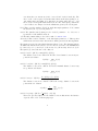
If X is a one-dimensional array, it is considered a condensed matrix of pairwise dissimilarities in the format which is returned by scipy.spatial.distance.pdist. It
contains the flattened, upper-triangular part of a pairwise dissimilarity matrix. That
is, if there are N data points and the matrix d contains the dissimilarity
( ) between the
i-th and j-th observation at position di,j , the vector X has length N2 and is ordered
as follows:

 

0 d0,1 d0,2 . . . d0,n−1
0 X[0]
X[1]
. . . X[n − 2]

 

0
d1,2 . . .
0
X[n − 1] . . .

 





0
...
0
...
d=
=





.
.
..
..

 

0
0
The metric argument is ignored in case of dissimilarity input.
The optional argument preserve_input specifies whether the method makes a working
copy of the dissimilarity vector or writes temporary data into the existing array. If the
dissimilarities are generated for the clustering step only and are not needed afterward,
approximately half the memory can be saved by specifying preserve_input=False.
Note that the input array X contains unspecified values after this procedure. It is
therefore safer to write
linkage(X, method="...", preserve_input=False)
del X
to make sure that the matrix X is not accessed accidentally after it has been used as
scratch memory. (The single linkage algorithm does not write to the distance matrix
or its copy anyway, so the preserve_input flag has no effect in this case.)
7
If X contains vector data, it must be a two-dimensional array with N observations in
D dimensions as an (N × D) array. The preserve_input argument is ignored in this
case. The specified metric is used to generate pairwise distances from the input. The
following two function calls yield equivalent output:
linkage(pdist(X, metric), method="...", preserve_input=False)
linkage(X, metric=metric, method="...")
The two results are identical in most cases, but differences occur if ties are resolved
differently: if the minimum in step 2 below is attained for more than one pair of
nodes, either pair may be chosen. It is not guaranteed that both linkage variants
choose the same pair in this case.
The general scheme of the agglomerative clustering procedure is as follows:
1. Start with N singleton clusters (nodes) labeled 0, . . . , N − 1, which represent the
input points.
2. Find a pair of nodes with minimal distance among all pairwise distances.
3. Join the two nodes into a new node and remove the two old nodes. The new
nodes are labeled consecutively N, N + 1, . . .
4. The distances from the new node to all other nodes is determined by the method
parameter (see below).
5. Repeat N − 1 times from step 2, until there is one big node, which contains all
original input points.
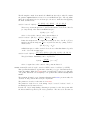
The output of linkage is stepwise dendrogram, which is represented as an (N − 1) ×
4 NumPy array with floating point entries (dtype=numpy.double). The first two
columns contain the node indices which are joined in each step. The input nodes are
labeled 0, . . . , N − 1, and the newly generated nodes have the labels N, . . . , 2N − 2.
The third column contains the distance between the two nodes at each step, ie. the
current minimal distance at the time of the merge. The fourth column counts the
number of points which comprise each new node.
The parameter method specifies which clustering scheme to use. The clustering scheme
determines the distance from a new node to the other nodes. Denote the dissimilarities
by d, the nodes to be joined by I, J, the new node by K and any other node by L.
The symbol |I| denotes the size of the cluster I.
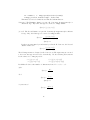
method='single': d(K, L) = min(d(I, L), d(J, L))
The distance between two clusters A, B is the closest distance between any two
points in each cluster:
d(A, B) = min d(a, b)
a∈A,b∈B
8
method='complete': d(K, L) = max(d(I, L), d(J, L))
The distance between two clusters A, B is the maximal distance between any
two points in each cluster:
d(A, B) =
max d(a, b)
a∈A,b∈B
|I| · d(I, L) + |J| · d(J, L)
|I| + |J|
The distance between two clusters A, B is the average distance between the
points in the two clusters:
method='average': d(K, L) =
d(A, B) =
1
|A||B|
∑
d(a, b)
a∈A,b∈B
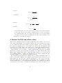
method='weighted': d(K, L) = 12 (d(I, L) + d(J, L))
There is no global description for the distance between clusters since the distance
depends on the order of the merging steps.
The following three methods are intended for Euclidean data only, ie. when X contains the pairwise (non-squared!) distances between vectors in Euclidean space. The
algorithm will work on any input, however, and it is up to the user to make sure that
applying the methods makes sense.
√
|I| · d(I, L) + |J| · d(J, L) |I| · |J| · d(I, J)
method='centroid': d(K, L) =
−
|I| + |J|
(|I| + |J|)2
There is a geometric interpretation: d(A, B) is the distance between the centroids
(ie. barycenters) of the clusters in Euclidean space:
d(A, B) = ∥⃗cA − ⃗cB ∥,
where ⃗cA denotes the centroid of the points in cluster A.
√
method='median': d(K, L) = 12 d(I, L) + 12 d(J, L) − 14 d(I, J)
Define the midpoint w
⃗ K of a cluster K iteratively as w
⃗ K = k if K = {k} is a
singleton and as the midpoint 21 (w
⃗I + w
⃗ J ) if K is formed by joining I and J.
Then we have
d(A, B) = ∥w
⃗A − w
⃗B∥
in Euclidean space for all nodes A, B. Notice however that this distance depends
on the order of the merging steps.
9
√
method='ward': d(K, L) =
(|I| + |L|) · d(I, L) + (|J| + |L|) · d(J, L) − |L| · d(I, J)
|I| + |J| + |L|
The global cluster dissimilarity can be expressed as
√
2|A||B|
d(A, B) =
· ∥⃗cA − ⃗cB ∥,
|A| + |B|
where ⃗cA again denotes the centroid of the points in cluster A.
fastcluster.single (X )
Alias for fastcluster.linkage (X, method='single').
fastcluster.complete (X )
Alias for fastcluster.linkage (X, method='complete').
fastcluster.average (X )
Alias for fastcluster.linkage (X, method='average').
fastcluster.weighted (X )
Alias for fastcluster.linkage (X, method='weighted').
fastcluster.centroid (X )
Alias for fastcluster.linkage (X, method='centroid').
fastcluster.median (X )
Alias for fastcluster.linkage (X, method='median').
fastcluster.ward (X )
Alias for fastcluster.linkage (X, method='ward').
fastcluster.linkage_vector (X, method='single', metric='euclidean', extraarg='None')
This performs hierarchical, agglomerative clustering on vector data with memorysaving algorithms. While the linkage method requires Θ(N 2 ) memory for clustering
of N points, this method needs Θ(N D) for N points in RD , which is usually much
smaller.
The argument X has the same format as before, when X describes vector data, ie. it is
an (N × D) array. Also the output array has the same format. The parameter method
must be one of 'single', 'centroid', 'median', 'ward', ie. only for these methods there
exist memory-saving algorithms currently. If method, is one of 'centroid', 'median',
'ward', the metric must be 'euclidean'.
Like the linkage method, linkage_vector does not treat NumPy’s masked arrays
as special and simply ignores the mask.
10
For single linkage clustering, any dissimilarity function may be chosen. Basically,
every metric which is implemented in the method scipy.spatial.distance.pdist
is reimplemented here. However, the metrics differ in some instances since a number
of mistakes and typos (both in the code and in the documentation) were corrected in
the fastcluster package.2
Therefore, the available metrics with their definitions are listed below as a reference.
The symbols u and v mostly denote vectors in RD with coordinates uj and vj respectively. See below for additional metrics for Boolean vectors. Unless otherwise stated,
the input array X is converted to a floating point array (X.dtype==numpy.double) if
it does has have already the required data type. Some metrics accept Boolean input;
in this case this is stated explicitly below.
'euclidean': Euclidean metric, L2 norm
d(u, v) = ∥u − v∥2 =
√∑
(uj − vj )2
j
'sqeuclidean': squared Euclidean metric
d(u, v) = ∥u − v∥22 =
∑
(uj − vj )2
j
'seuclidean': standardized Euclidean metric
√∑
d(u, v) =
(uj − vj )2 /Vj
j
The vector V = (V0 , . . . , VD−1 ) is given as the extraarg argument. If no extraarg
is given, Vj is by default the unbiased sample
of all observations in
∑ variance
2
the j-th coordinate, Vj = Vari (Xi,j ) = N 1−1 i (Xi,j
− µ(Xj )2 ). (Here, µ(Xj )
denotes as usual the mean of Xi,j over all rows i.)
'mahalanobis': Mahalanobis distance
√
d(u, v) =
(u − v)⊤ V (u − v)
Here, V = extraarg, a (D × D)-matrix. If V is not specified, the inverse of the
covariance matrix numpy.linalg.inv(numpy.cov(X, rowvar=False)) is used:
1 ∑
(V −1 )j,k =
(Xi,j − µ(Xj ))(Xi,k − µ(Xk ))
N −1 i
2 Hopefully,
the SciPy metric will be corrected in future versions and some day coincide with the fastcluster
definitions. See the bug reports at http://projects.scipy.org/scipy/ticket/1484, http://projects.
scipy.org/scipy/ticket/1486.
11
'cityblock': the Manhattan distance, L1 norm
∑
d(u, v) =
|uj − vj |
j
'chebychev': the supremum norm, L∞ norm
d(u, v) = max |uj − vj |
j
'minkowski': the Lp norm

d(u, v) = 
∑
1/p
|uj − vj |p 
j
This metric coincides with the cityblock, euclidean and chebychev metrics for
p = 1, p = 2 and p = ∞ (numpy.inf), respectively. The parameter p is given as
the 'extraarg' argument.
'cosine'
∑
⟨u, v⟩
j uj vj
d(u, v) = 1 −
= 1 − √∑
∑ 2
∥u∥ · ∥v∥
2
j vj
j uj ·
'correlation': This method first mean-centers the rows of X and then applies the
cosine distance. Equivalently, the correlation distance measures 1 − (Pearson’s
correlation coefficient).
d(u, v) = 1 −
⟨u − µ(u), v − µ(v)⟩
,
∥u − µ(u)∥ · ∥v − µ(v)∥
'canberra'
d(u, v) =
∑ |uj − vj |
|uj | + |vj |
j
Summands with uj = vj = 0 contribute 0 to the sum.
'braycurtis'
∑
j
d(u, v) = ∑
j
|uj − vj |
|uj + vj |
(user function): The parameter metric may also be a function which accepts two
NumPy floating point vectors and returns a number. Eg. the Euclidean distance
could be emulated with
12
fn = lambda u, v: numpy.sqrt(((u-v)*(u-v)).sum())
linkage_vector(X, method='single', metric=fn)
This method, however, is much slower than the built-in function.
'hamming': The Hamming distance accepts a Boolean array (X.dtype==bool) for
efficient storage. Any other data type is converted to numpy.double.
d(u, v) = |{j | uj ̸= vj }|
'jaccard': The Jaccard distance accepts a Boolean array (X.dtype==bool) for efficient
storage. Any other data type is converted to numpy.double.
d(u, v) =
|{j | uj ̸= vj }|
|{j | uj ̸= 0 or vj ̸= 0}|
d(0, 0) = 0
Python represents True by 1 and False by 0. In the Boolean case, the Jaccard
distance is therefore:
|{j | uj ̸= vj }|
d(u, v) =
|{j | uj ∨ vj }|
The following metrics are designed for Boolean vectors. The input array is converted
to the bool data type if it is not Boolean already. Use the following abbreviations
for the entries of a contingency table:
a = |{j | uj ∧ vj }|
c = |{j | (¬uj ) ∧ vj }|
b = |{j | uj ∧ (¬vj )}|
d = |{j | (¬uj ) ∧ (¬vj )}|
Recall that D denotes the number of dimensions, hence D = a + b + c + d.
'yule'
d(u, v) =
2bc
ad + bc
'dice'
b+c
2a + b + c
d(0, 0) = 0
d(u, v) =
'rogerstanimoto'
d(u, v) =
13
2(b + c)
b+c+D
'russellrao'
d(u, v) =
b+c+d
D
'sokalsneath'
2(b + c)
a + 2(b + c)
d(0, 0) = 0
d(u, v) =
'kulsinski'
1
d(u, v) = ·
2
(
c
b
+
a+b a+c
)
'matching'
b+c
D
Notice that when given a Boolean array, the matching and hamming distance
are the same. The matching distance formula, however, converts every input to
Boolean first. Hence, the vectors (0, 1) and (0, 2) have zero matching distance
since they are both converted to (False, True) but the hamming distance is 0.5.
d(u, v) =
'sokalmichener' is an alias for 'matching'.
3 Behavior for NaN and infinite values
Whenever the fastcluster package encounters a NaN value as the distance between nodes,
either as the initial distance or as an updated distance after some merging steps, it raises
an error. This was designed intentionally, even if there might be ways to propagate NaNs
through the algorithms in a more or less sensible way. Indeed, since the clustering result
depends on every single distance value, the presence of NaN values usually indicates a
dubious clustering result, and therefore NaN values should be eliminated in preprocessing.
In the R interface for vector input, coordinates with NA value are interpreted as missing
data and treated in the same way as R’s dist function does. This results in valid output
whenever the resulting distances are not NaN. The Python interface does not provide any
way of handling missing coordinates, and data should be processed accordingly and given
as pairwise distances to the clustering algorithms in this case.
The fastcluster package handles node distances and coordinates with infinite values correctly, as long as the formulas for the distance updates and the metric (in case of vector
input) make sense. In concordance with the statement above, an error is produced if a
NaN value results from performing arithmetic with infinity. Also, the usual proviso applies:
internal formulas in the code are mathematically equivalent to the formulas as stated in the
documentation only for finite, real numbers but might produce different results for ±∞.
14
Apart from obvious cases like single or complete linkage, it is therefore recommended that
users think about how they want infinite values to be treated by the distance update and
metric formulas and then check whether the fastcluster code does exactly what they want
in these special cases.
4 Differences between the two interfaces
• The 'mcquitty' method in R is called 'weighted' in Python.
• R and SciPy use different conventions for the “Euclidean” methods 'centroid', 'median' and 'Ward'! R assumes that the dissimilarity matrix consists of squared Euclidean distances, while SciPy expects non-squared Euclidean distances. The fastcluster package respects these conventions and uses different formulas in the two
interfaces.
If the same results in both interfaces ought to be obtained, then the hclust function in
R must be fed with the entry-wise square of the distance matrix, d^2, for the 'ward',
'centroid' and 'median' methods, and later the square root of the height field in
the dendrogram must be taken. The hclust.vector method calculates non-squared
Euclidean distances, like R’s dist method and the Python interface. See the example
in the hclust.vector documentation above.
For the 'average' and 'weighted' alias 'mcquitty' methods, the same, non-squared
distance matrix d as in the Python interface must be used for the same results. The
'single' and 'complete' methods only depend on the relative order of the distances,
hence it does not make a difference whether the method operates on the distances or
the squared distances.
The code example in the R documentation (enter ?hclust or example(hclust) in
R) contains another instance where the squared distance matrix is generated from
Euclidean data.
• The Python interface is not designed to deal with missing values, and NaN values
in the vector data raise an error message. The hclust.vector method in the R
interface, in contrast, deals with NaN and the (R specific) NA values in the same way
as the dist method does. Confer the documentation for dist for details.
5 References
NumPy: Scientific computing tools for Python, http://numpy.scipy.org/.
Eric Jones, Travis Oliphant, Pearu Peterson et al., SciPy: Open Source Scientific Tools for
Python, 2001, http://www.scipy.org.
15
R: A Language and Environment for Statistical Computing, R Foundation for Statistical
Computing, Vienna, 2011, http://www.r-project.org.
16