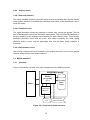
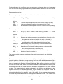
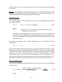
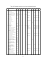
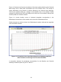
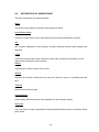
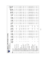
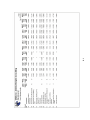
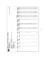
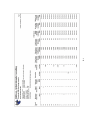
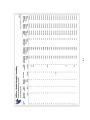
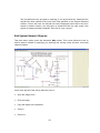
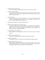
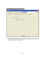
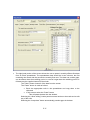
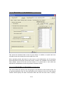
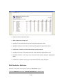
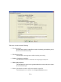
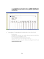
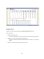
Download a model for rapidly assessing the impact of waste discharge on

A MODEL FOR RAPIDLY ASSESSING THE IMPACT OF
WASTE DISCHARGE ON DOWNSTREAM WATER QUALITY
Report to the
Water Research Commission
by
CE Herold1, K le Roux2, J Blight3, A Rowse3 and S Dladla3
1
Umfula Wempilo Consulting
2
Datron Electronic Systems
3
Department of Civil Engineering
University of the Witwatersrand
WRC Report No. 1212/1/10
ISBN 978-1-77005-986-3
August 2010
DISCLAIMER
This report has been reviewed by the Water Research Commission (WRC) and
approved for publication. Approval does not signify that the contents necessarily reflect
the views and policies of the WRC, nor does mention of trade names or commercial
products constitute endorsement or recommendation for use.
EXECUTIVE SUMMARY
INTRODUCTION
Background and motivation
DWA Regional Office, Head Office and CMA staff needs a rapid means of assessing the
impact of waste load discharge permit applications and the required degree of change to
permit conditions to meet water quality objectives. WQ2000 already provides such a tool for
salinity. However, non-conservative pollutants are also of paramount importance to water
quality managers. This is because human activities typically result in the discharge of
nutrients and biological pollutant loads, thereby promoting eutrophication of water bodies and
presenting a direct threat to public health. A number of models are available for simulating
these impacts. However, they are generally highly complex, data intensive and costly to
apply, requiring the services of experts to set up and test each and every option. In practice,
the use of such models is usually defeated by shortage of funds, excessive development
time delays and the fact that such complex models seldom deliver commensurately adequate
results.
Another important factor is that water quality models require naturalised catchment flow data
to provide essential input. Processing of this essential hydrological data requires extensive
patching and analysis. Typically several years elapse between the major studies required to
produce this data. This means that the water quality data collected in the interim cannot be
used effectively to answer the key “what if?” questions such as, “what will happen if a new
effluent source is introduced?” This is especially important since our water quality data base
is relatively short.
This research is aimed at providing a simple to apply evaluation tool capable of making good
use of the new water quality data and of simulating the effects of both conservative and nonconservative pollutants, taking account of both point and diffuse inputs. This model requires
experts to first set up the model, after which the CMA and Regional Office personnel can use
it to rapidly test a range of waste discharge options with minimal input from experts. The
objective is to speed up and reduce the cost of processing waste discharge applications and
the testing of alternative discharge permits. Departmental personnel and scarce outside
experts should then be freed to concentrate on interpreting the model output data, setting
appropriate permit levels, filling key data gaps and ensuring compliance with the
requirements.
Aims
1.
Provide a simple to apply model for rapidly assessing the impact of applications for
new waste load discharges, or applications for the modification of old permits.
2.
Calibrate and test the model on an existing river system. The Blesbokspruit
catchment has been chosen for this purpose.
iii
3.
Provide adequate documentation of the model.
Approach
A model has been developed to utilise the most recent flow and water quality data available in
standard DWA hydrological and water quality data systems without any need for prior
processing or naturalisation. User-friendly screens have been provided to facilitate system
setup and the capture of river channel data. The model is self-calibrating. The simulation mode
provides a powerful tool for assessing the impact of system changes on the water quality in
downstream channel reaches. The statistical properties of the stored calibrated river channel
decay values, diffuse input loads and effluent concentrations are used to generate stochastic
values that are used in the simulation mode during which concentrations are generated at the
ends of each channel reach for a range of flow conditions. The results are then tabulated and
plotted against defined water quality objectives.
Applications
Key applications include:



Rapid assessment of impacts of waste discharge
Initial testing of management options
Evaluation of monitoring requirements
WQDOWN MODEL
WQDown is a simple to operate self-calibrating non-conservative variable water quality model
that was developed to simulate the effect of applications for new waste discharge permits (or
changes to existing permits) on downstream water quality.
Model concept
The main steps in the modelling process are outlined in Figure 1. These are discussed below.
1. Define run: Select an existing project database or create a new one.
2. Set up system: Set up the catchment layout, system network and channel reach
characteristics and define the flow and water quality input files. The initial setup requires
specialist input, but need not be repeated unless substantial changes are made to the system.
3. Select water quality variable: A selection is made from the water quality variables
contained in the data files generated by the DWA’s Water Management System (WMS).
iv
1. Define Run:
Select existing system or
define new one
2. Set up system consisting
of connecting channel reaches
3. Select water quality variable
5. Simulation
4. Calibration
4.1 Specify water quality data
5.1 Define simulation attributes:
4.3 Estimate incremental catchment
runoffs and channel reach losses
- Simulation period
- Number of repetitions
- Urban and irrigation areas
- Point discharges
- Mean effluent concentrations
- Characteristics for new effluent sources
- Residual distribution type
4.4 Calculate runoff adjustment factor:
Compare estimated flow with observed flow
at gauging weir and calculate catchment
runoff adjustment factor
5.2 Calculate channel
reach flows
4.6 Calculate channel reach detention times
5.3 Stochastic selection: Of effluent
source concentrations, reach decay
values and reach diffuse input loads
Daily loop
4.5 Adjust estimated incremental
catchment runoffs: To all channel reaches
and ensuing channel reach flows
.
Repetition loop
Loop for selected days
4.2 Select calibration dates:
Days with observed flow and
sufficient water quality values
5.4 Calculate concentration
at end of each channel reach
4.7 Calculate decay value or diffuse
diffuse input for each channel reach
6. Display Results
4.8 Accumulate statistics: For point source
Inputs, decay values and diffuse input loads
6.1 Calculate statistics
6.2 Tabulate
results
4.9 Calculate stochastic parameters
Simulate new option
6.3 Plot
duration curves
Select?
New variable
Figure 1: Main steps in the WQDown modelling process
v
End
End
4. Calibration: Define and run model calibration.
Calibration setup includes:
 Specify water quality data and default values
 Select calibration dates based on availability of flow and water quality data.
For each calibration date the model automatically does the following:
 Estimates incremental catchment runoffs and channel reach losses
 Calculates runoff adjustment factor: The initial flow estimate at the downstream end of
the channel reach coinciding with the catchment flow gauging station is compared with
the observed flow to yield an adjustment factor
 Adjust estimated incremental catchment runoffs: The adjustment factor is applied to all
of the previously calculated initial incremental catchment runoffs
 Calculate channel reach detention times
 Calculate decay value or diffuse input for each channel reach
 Accumulate statistics: for decay values and diffuse inputs to each channel reach.
After completion of the main simulation loop the stochastic parameters are calculated for each
channel reach and effluent point source and a statistical summary is generated.
5. Simulation: Define and run model simulation.
Simulation setup includes:
 Define simulation attributes: Set up the system attributes defining the simulation run
including simulation period, number of repetitions, urbanised and irrigated areas,
effluent discharge flow and water quality characteristics, abstraction rates and
parameters controlling the handling of the stochastically generated residuals for effluent
concentrations and channel reach decay values and diffuse load inputs.
For each iterated day of the simulation period the model automatically does the following:
 Calculate channel reach flows and detention times
 Stochastic selection: of effluent concentration, channel reach decay or diffuse input
load for each channel reach
 Calculate concentration at end of each channel reach.
6. Display results: The mean, standard deviation, percentile values and the percentage
time that the defined water quality objective is exceeded are calculated and stored at the
downstream end of each river reach. The following types of display are provided:
 Tabulate results
 Plot duration curves: for one or more channel reaches, along with the water quality
objective.
Model Algorithms
The algorithms used in model calibration and model simulation are described.
vi
DATA REQUIREMENTS
The data requirements for WQDown have been divided into three groups:
 Initial setup
 Periodic updating
 Simulation.
Initial setup
This step should be carried out by persons with expertise in hydrological and water quality
modelling. User-friendly screens have been provided to facilitate this. The following information
is required for the initial model setup:
 Reference gauge flow data
 Define system network
 Channel reach data:
Quaternary location
Channel length
Channel flow control data
Mean monthly values
Point discharge and abstraction flow data
River sampling water quality data (WMS files)
Effluent quality data (WMS files) and default concentrations
Controls defining calibration period, default values, etc.
Set standard dates
Periodic updating
Periodic updating falls into two classes:
 Revision of the setup: Done after significant catchment changes and requires modelling
expertise.
 Updating of time series data: Updating of river flow and WMS water quality time series
files and monthly point source discharge and abstraction flow data. It is also desirable to
regularly (say each year) re-evaluate the default effluent point source concentration decay
values. These updates can be carried out by competent Head Office, Regional Office and
CMA personnel who have had appropriate training and is desirable once per year.
Simulation
Model simulation is the intended day by day use of the model by Regional Office and CMA
personnel. The data that is required for simulation relates only to the system change being
simulated.
vii
TESTING ON BLESBOKSPRUIT CATCHMENT
The model was tested on the Blesbokspruit catchment and the lower portion of the
Suikerbosrand River down to its confluence with the Vaal River.
This system was chosen for model testing because it contains all of the main elements used in
WQDown, including heavily urbanised, irrigation, wetland and lake features, several effluent
point sources, water abstractions, diffuse pollution from a number of areas, several river and
effluent water quality monitoring stations of various sampling frequency and duration and a flow
gauging station. The catchment is also of great concern due to high pollution load inputs, the
Blesbokspruit RAMSAR wetland, the threat posed to informal users who may use the river
water for domestic purposes and the impact on the already polluted Vaal Barrage and
downstream Middle Vaal River.
Model testing comprised simulation of phosphate for two options:
 Baseline
 Grootvlei Gold Mine effluent ceases.
Cessation of Grootvlei Gold Mine underground effluent results in an 82% increase in the
simulated 90-percentile peak phosphate concentration at the Grootvlei Mine bridge (to 0.89
mg/l), with a 70% increase in the mean (to 0.35 mg/l). near the downstream end of the wetland
at the R42 road crossing the increase in the simulated 90-percentile peak reduced to 67% and
the mean to 39%. Near the mouth of the Suikerbosrand River at weir C2H004 the increase in
the 90-percentile rose to 95%, although the absolute magnitude of the peak reduced to 0.76
mg/l, while the mean increased by 34%.
This example demonstrates the potential of WQDown for making rapid initial assessments of
the impact of changes in waste discharges on water quality in complex systems.
MODEL CAPABILITIES AND LIMITATIONS
Model capabilities

Rapid initial assessment: WQDown places a powerful tool in the hands of water
resource managers to make rapid “what if?” assessments of the impact of a variety of
options on the concentrations of non-conservative and conservative pollutants in complex
river systems.

User friendly: The user-friendly features are designed to permit managers who do not
have detailed experience in water quality modelling to apply it.

Automatic calibration: A particular strength and unique feature of WQDown is that it is
self-calibrating and makes full use of the available water quality records and streamflow
data routinely processed by the DWA. The technique employed to seamlessly naturalise
the hydrology is a strong feature. A third unique feature is the method of switching between
viii
the calculation of decay values and diffuse input loads and the use of stochastic modelling
to sample these values in the simulation mode. Treating the decay and diffuse loads as
stochastic elements, rather than the conventional method of running water quality
concentrations through a stochastic generator lifts the model from a blind regression
process to a tool that can take account of cause and effect.

Assess complex systems using limited data:
The model has been tested on an
extremely complex and highly developed river system and used to evaluate one of a wide
variety of options. The test produced plausible results.
Model Limitations

Initial evaluation: WQDown is intended as an initial rapid assessment tool. It is not
meant to replace more comprehensive models. However, it must be stated that more
comprehensive models are impractical to apply in most instances due to their insatiable
data requirements.

Probabilistic model: WQDown is a hybrid between process modelling with relatively
simple decay and stochastic generation. It telescopes all of the complex in-stream
processes into simple decay and, where appropriate, diffuse input. As such the model
remains agnostic about the type of channel reach (wetland, lake or normal river channel),
sedimentation, sediment uptake, organic cycling, etc. All these are covered by a single
decay factor calculated for the entire channel reach.
Comprehensive water quality models require the laborious calibration of fixed decay and other
parameter values, resulting in compromise values that fail to simulate observed extremes and
therefore inevitably under-estimate the observed variance. By contrast WQDown preserves the
variance by treating the calculated decay values as a stochastically changing variable that is a
feature of each channel reach. The complex inter-relationship between all of the parameters
and processes playing a part in the channel reach often defeats complex modelling. This is
because extreme water quality events in a real system tend to be dominated by unanticipated
events, such as sewer overflows, illegal discharges, temporary biological failure of a sewage
works when unexpected slugs of toxic waste enter the sewers, chlorine dosing plant failure and
the like. Even the most sophisticated models cannot hope to replicate such semi-stochastic
events. However, the characteristics are contained in the river quality data. WQDown uses this
information in such a way that the statistical properties are preserved, but also allows a variety
of management options to be simulated in a rational way.
The underlying assumption is that the gross dynamics of the channel reach will remain
unchanged. If the channel reach characteristics are radically altered, for example if a wetland is
canalised or a lake breached, then the decay down the channel reach will also be altered. The
model is flexible enough to permit the assigning of a default decay value for the channel reach
that corresponds to the characteristics of another water body. So, for example, if a new lake is
developed, then the default decay value for a similar lake can be applied to the channel reach
and at the same time the earlier water quality data record for the channel reach (if such exists)
can be discarded thereby forcing use of the new default value. Then, as more sampling data is
ix
accumulated by the regular data collection programme, the old inapplicable data for the
channel reach can be replaced by the new data that represents the altered condition.
USER MANUAL
A user manual dealing with model setup and describing the mechanics of using the model is
provided.
CONCLUSIONS
The following conclusions have been drawn.
Aims achieved



A simple to apply self-calibrating model for rapidly assessing the impact of proposed waste
load discharges on river system non-conservative water quality has been provided.
The model has been calibrated and tested successfully on the highly developed and
complex Blesbokspruit catchment.
The model has been documented.
Data requirements defined
The data requirements of the WQDown model have been defined and differentiated between
the needs for:
 Once-off initial setup by modelling specialists
 Periodic revision of the setup to reflect changing conditions
 Ongoing application by Regional Office and CMA personnel.
All of the data is well within the means of the parties concerned to assimilate from readily
available sources.
Dissemination and application
Incorporation in the DWA’s User Support System and associated training will ensure that the
vast potential benefits of this unique modelling tool are fully realised. Catchments where there
is already a pressing need to apply the model have been identified.
Further research needs
Beneficial research needs have been identified to further facilitate the application of the model.
x
RECOMMENDATIONS
Dissemination and application
The primary purpose of WQOWN is to aid in the evaluation of discharge permits and generally
assist in assessing catchment management strategies. Accordingly the following actions
should be put into effect without undue delay.

Incorporate in User Support System:
DWA’s User Support System (USS).

Training: Training sessions should be set up to ensure that the new technology is widely
disseminated..

Application: There are immediate areas of application where the model can be used,
including, but not limited to, the following developed catchments:
Blesbokspruit
Klip River
Rietspruit
Vaal Barrage
Waterval River
Mgeni River
Crocodile River (West)
Mooi River

Rationalise water quality monitoring:
The model could be used to rationalise
monitoring programmes to better serve the needs of water quality modelling:
WQDOOWN should be incorporated into the
Further research

Automatic convergence of default values:
A procedure to automatically reset the
default decay values based on the average simulated for the available sample points is
desirable.

Include temperature effects: Temperature plays a significant role in in-stream decay
processes and should be incorporated.

Assign decay distributions to unmonitored channel reaches: At present the decay
rates for unmonitored channel reaches are assumed to remain constant at the defined
default value. However, a better approach might be to link the unmonitored channel reach
to a suitable nearby route that has similar characteristics. In the calibration mode the decay
value calculated for the associated channel reach could then be used in place of the default
value for dates when data is available for the associated channel reach.
xi

Merge routes for calculating decay values:
It often occurs that two water quality
monitoring points are separated by more than one channel reaches to accommodate point
inputs or river junctions. Grouping of similar stations along portions of river lengths could
facilitate direct calculation of decay values for the entire channel reach.

Increase simulation speed:
speed.

Growth in historical catchment development: Allowing for growth between specified
break point values is recommended.

Introduce variable seasonal effluent flow: A facility to use the monthly point discharge
and abstraction time series calibration data to derive a dimensionless monthly seasonal
pattern for use in the simulation mode is recommended.

Track calibration changes: Checks are required to determine when last the river flow
and WMS files and project database were updated and the time and date of the latest
calibration run to obviate unnecessary repetition of the calibration step.

Combine water quality records: It has been observed that the WMS database contains
two and sometimes three feature codes for the same monitoring point. Since these split the
record over different periods it is important to combine them for the purpose of modelling.

Sensitivity analyses: Sensitivity analyses are required to determine:
The desired number of repetitions of the hydrology to ensure convergence
during model simulation
The effect that the choice of distribution type (linear, log or observed) has on
simulated water quality
Determine how seasonality affects the simulation results
The effect of eliminating poor and small or redundant records, rather than letting
them dilute long channel reaches with default values.

Relate catchment quality to runoff:
The concentration assumed for incremental
catchment runoff can affect the modelling of decay rates and diffuse input loads. Derivation
of suitable relationships between incremental runoff and runoff quality is desirable.

Test other water quality variables:
The initial model development and testing has
focussed on phosphate. Other water quality variables should be tested. This is probably
best linked to the practical application of the model, rather than as an academic exercise.

Simulate for exact calibration dates and flow conditions and compare water quality
statistics:
Checking for complex systems would be enabled by a facility to run a
simulation that exactly replicates the flow conditions of the calibration period, using the
identical dates and the corresponding effluent and abstraction discharge rates.
Various means are available to increase the simulation
xii

Update WR90 with WR2005 quaternary data: Replacement of the WR90 values in the
database with data from the WR2005 study is recommended, together with the unit paved
surface runoff proportions.

Incorporate multiple flow gauges:
desirable.

Effect of storage:
WQDown is not a dynamic model. Storage effects in large
impoundments may warrant investigation.

Integrate with WMS:
consideration.
The inclusion of multiple flow gauging points is
Integration of WQDown into the DWA’s WMS system bears
xiii
ACKNOWLEDGEMENTS
The research in this report emanated from a project funded by the Water Research
Commission and is entitled: "Development of a user-friendly model for assessing the
impact of waste discharge applications on downstream water quality".
The Steering Committee responsible for this project consisted of:
Mr HM du Plessis
Mr H Maaren
Mr M Keet
Mr P Viljoen
Mr G Grobler
Mr M Selepe
Mr F van Wyk
Mr S Terry
Mr DA Salmon
Dr CE Herold
Water Research Commission (Chairman)
Water Research Commission
Department of Water Affairs, Gauteng Region
Department of Water Affairs, Resource Planning Systems –
Water Quality Planning
Department of Water Affairs, Resource Planning Systems –
Water Quality Planning
Department of Water Affairs, Gauteng Region
Rand Water
Umgeni Water
Anglo Coal Environmental Services
Stewart Scott Water Quality
The financing of the project by the Water Research Commission and the contribution of
the members of the Steering Committee are gratefully acknowledged.
This project was only possible with the co-operation of many individuals and institutions.
In this regard the authors wish to record their sincere thanks to Ms R Munnik of the
Department of Water Affairs for the provision of water quality data. Mr J van Wyk, C
Swanepoel, Ms D Maritz, B Davis and M Erasmus of the Department of Water Affairs
also offered valuable advice and information regarding the Water Management System.
xiv
TABLE OF CONTENTS
Page
EXECUTIVE SUMMARY ......................................................................................................
iii
ACKNOWLEDGMENTS ...................................................................................................... xiv
TABLE OF CONTENTS .......................................................................................................
xv
LIST OF FIGURES ...............................................................................................................
xx
LIST OF TABLES ................................................................................................................. xxi
LIST OF ABBREVIATIONS ................................................................................................ xxii
1.
INTRODUCTION ......................................................................................................
1
1.1
Background and motivation ......................................................................................
1
1.2
Aims
.....................................................................................................................
3
1.3
Approach ...................................................................................................................
3
1.4
Applications ...............................................................................................................
1.4.1
Rapid assessment of impacts of waste discharge ...................................
1.4.2
Initial testing of management options ........................................................
1.4.3
Evaluation of monitoring requirements .......................................................
4
4
4
4
1.5
Structure of the report ...............................................................................................
5
2.
WQDOWN MODEL ..................................................................................................
6
2.1
Literature survey .......................................................................................................
6
2.2
Model concept ...........................................................................................................
2.2.1
Define run ...................................................................................................
2.2.2
Set up system .............................................................................................
2.2.3
Select water quality variables ....................................................................
2.2.4
Calibration .................................................................................................
2.2.4.1 Specify water quality data ...........................................................
2.2.4.2 Select calibration dates ...............................................................
6
6
6
8
8
8
9
xv
TABLE OF CONTENTS
Page
2.2.5
2.2.6
2.2.4.3 Estimate incremental catchment runoffs and channel reach
Losses .........................................................................................
2.2.4.4 Calculate runoff adjustment factor ...............................................
2.2.4.5 Adjust estimated incremental catchment runoffs ........................
2.2.4.6 Calculate channel reach detention times ....................................
2.2.4.7 Calculate decay value or diffuse input for each channel reach ...
2.2.4.8 Accumulate statistics ...................................................................
2.2.4.9 Calculate stochastic parameters and generate statistical
summaries ..................................................................................
Simulation ..................................................................................................
2.2.5.1 Define simulation attributes ..........................................................
2.2.5.2 Calculate channel reach flows .....................................................
2.2.5.3 Stochastic selection .....................................................................
2.2.5.4 Calculate concentrations at ends of channel reach ....................
Display results ...........................................................................................
2.2.6.1 Calculate statistics .......................................................................
2.2.6.2 Tabulate results ............................................................................
2.2.6.3 Plot duration curves .....................................................................
9
9
10
10
10
11
11
11
11
13
14
14
15
15
15
15
2.3
Model structure .........................................................................................................
2.3.1
Overview .....................................................................................................
2.3.2
Catchment representation ..........................................................................
2.3.3
Channel reach representation ....................................................................
15
15
16
18
2.4
Calibration algorithms ...............................................................................................
2.4.1
Point source inputs and abstractions .........................................................
2.4.2
Channel reach flow .....................................................................................
2.4.3
Velocity- flow relationships .........................................................................
2.4.4
Detention time ............................................................................................
2.4.5
Water quality at head of channel reach .....................................................
2.4.6
In-stream attenuation between pairs of points ...........................................
2.4.7
Accumulation of statistics ...........................................................................
19
19
20
26
29
30
31
33
2.5
Simulation algorithms ...............................................................................................
2.5.1
Initialisation .................................................................................................
2.5.2
Run simulation .............................................................................................
2.5.2.1 Simulation of effluent concentrations ...........................................
2.5.2.2 Simulation of decay values ..........................................................
2.5.2.3 Simulation of diffuse loads ...........................................................
34
34
34
35
37
38
xvi
TABLE OF CONTENTS
Page
2.5.3
2.5.2.4 Calculation of downstream concentration ................................... 40
Presentation of results................................................................................. 40
3.
DATA REQUIREMENTS ......................................................................................... 41
3.1
Initial setup ................................................................................................................
3.1.1
Reference gauge flow data ........................................................................
3.1.2
Define system network ...............................................................................
3.1.3
Channel reach data ....................................................................................
3.2
Periodic updating ...................................................................................................... 44
3.2.1
Revision of setup ........................................................................................ 44
3.2.2
Updating of time series data ...................................................................... 44
3.3
Simulation ................................................................................................................. 45
4.
TESTING ON BLESBOKSPRUIT CATCHMENT ................................................... 47
4.1
Introduction ............................................................................................................... 47
4.2
Catchment overview .................................................................................................
4.2.1
Initialisation ..................................................................................................
4.2.2
Reference flow gauge .................................................................................
4.2.3
System network ..........................................................................................
4.2.4
River reach attributes .................................................................................
4.2.5
River reach quality data .............................................................................
4.2.6
Point source data .......................................................................................
4.3
Calibration results ..................................................................................................... 58
4.4
Model results ............................................................................................................. 58
4.4.1
Baseline ...................................................................................................... 58
4.4.2
Grootvlei Gold Mine discharge ceases ....................................................... 61
5.
MODEL CAPABILITIES AND LIMITATIONS ......................................................... 65
5.1
Model capabilities .....................................................................................................
5.1.1
Rapid initial assessment ............................................................................
5.1.2
User friendly ...............................................................................................
5.1.3
Automatic calibration ..................................................................................
xvii
41
41
41
41
47
47
52
52
52
52
52
65
65
65
65
TABLE OF CONTENTS
Page
5.1.4
Assess complex systems using limited data ............................................. 65
5.2
Model limitations ....................................................................................................... 65
5.2.1
Initial evaluation .......................................................................................... 65
5.2.2
Probabilistic model ..................................................................................... 66
6.
USER MANUAL ....................................................................................................... 67
7.
CONCLUSIONS ....................................................................................................... 68
7.1
Aims achieved ........................................................................................................... 68
7.2
Data requirements defined ....................................................................................... 68
7.3
Dissemination and application .................................................................................. 68
7.4
Further research needs ............................................................................................ 68
8.
RECOMMENDATIONS ............................................................................................ 69
8.1
Dissemination and application ...................................................................................
8.1.1
Incorporate in User Support System ..........................................................
8.1.2
Training .......................................................................................................
8.1.3
Application ...................................................................................................
8.1.3.1 Blesbokspruit ................................................................................
8.1.3.2 Klip River ......................................................................................
8.1.3.3 Rietspruit ......................................................................................
8.1.3.4 Vaal Barrage ................................................................................
8.1.3.5 Waterval .......................................................................................
8.1.3.6 Mgeni River ..................................................................................
8.1.3.7 Crocodile River .............................................................................
8.1.3.8 Mooi River ....................................................................................
8.1.4
8.2
69
69
69
69
69
69
70
70
70
70
70
70
Rationalise water quality sampling ............................................................. 71
Further research ........................................................................................................
8.2.1
Automatic convergence of default values ..................................................
8.2.2
Include temperature effects ........................................................................
8.2.3
Assign decay distribution to unmonitored reaches ....................................
8.2.4
Merge routes for calculating decay values ................................................
xviii
72
72
72
73
73
TABLE OF CONTENTS
Page
8.2.5
8.2.6
8.2.7
8.2.8
8.2.9
8.2.10
8.2.11
8.2.12
8.2.13
8.2.14
8.2.15
8.2.16
8.2.17
9.
Increase simulation speed .........................................................................
Growth in historical catchment development .............................................
Introduce variable effluent flow ..................................................................
Track calibration changes ..........................................................................
Combine water quantity records ................................................................
Sensitivity analyses ....................................................................................
Relate catchment quality to runoff .............................................................
Test other water quality variables ..............................................................
Simulate for exact calibration dates and flow conditions and
compare water quality statistics ................................................................
Update WR90 with WR2005 quaternary data ..........................................
Incorporate multiple flow gauges ...............................................................
Effect of storage .........................................................................................
Integrate with WMS ....................................................................................
74
74
75
75
75
76
76
77
77
77
78
78
78
REFERENCES ......................................................................................................... 79
APPENDIX A: WQDOWN SUBROUTINES ..................................................................... A.1
APPENDIX B: WQDOWN CALIBRATION RESULTS FOR BLESBOKSPRUIT ............. B.1
APPENDIX C: WQDOWN SIMULATION RESULTS FOR BLESBOKSPRUIT
BASELINE CONDITION ........................................................................... C.1
APPENDIX D: WQDOWN SIMULATION RESULTS FOR BLESBOKSPRUIT
GROOTVLEI GOLD MINE DISCHARGE CEASES ................................ D.1
APPENDIX E: USER MANUAL ........................................................................................ E.1
xix
LIST OF FIGURES
Page
2.1
Main steps in the WQDown modelling process .......................................................
2.2
Overview of model structure ..................................................................................... 15
2.3
Typical catchment layout .......................................................................................... 16
2.4
Model system configuration ...................................................................................... 17
2.5
Channel reach configuration...................................................................................... 18
2.6
Lake outlet section .................................................................................................... 28
2.7
Decay with introduction of diffuse input load ............................................................ 32
4.1
Blesbokspruit catchment .......................................................................................... 48
4.2
North-West section of Blesbokspruit catchment ...................................................... 49
4.3
Central section of Blesbokspruit catchment ............................................................. 50
4.4
South-West section of Blesbokspruit catchment ...................................................... 51
4.5
Blesbokspruit catchment system network ................................................................ 53
4.6
Duration curves of phosphate along the Benoni canal ............................................ 59
4.7
Phosphate in the upper Blesbokspruit – Baseline option ........................................ 60
4.8
Phosphate in the Blesbokspruit wetland – Baseline option ..................................... 61
4.9
Phosphate in the lower Blesbokspruit and Suikerbosrand River
– Baseline option ...................................................................................................... 62
4.10
Phosphate in the Blesbokspruit wetland – After cessation of discharge from
Grootvlei Gold Mine .................................................................................................. 62
4.11
Phosphate in the lower Blesbokspruit and Suikerbosrand River
– After cessation of discharge from Grootvlei Gold Mine ........................................ 63
xx
7
LIST OF TABLES
Page
4.1
Attributes of Blesbokspruit system network ............................................................. 54
4.2
Phosphate and point source input and abstraction data .......................................... 57
4.3
Changes in phosphate concentration after cessation of Grootvlei discharge ......... 64
xxi
LIST OF ABBREVIATIONS
CMA
Catchment Management Agency
DWA
Department of Water Affairs
USS
User Support System
VRSAU
DWA Vaal River System Analysis Update study
WMS
Water Management System (DWA water quality system)
WQDown
Water quality assessment model developed in this project
WQT
Water Quality TDS (and sulphate) monthly catchment model
WQ2000
User-friendly system for rapidly assessing salinity in quaternary catchments
making use of the a pre-calibrated version of the WQT hydro-salinity model
WR2005
Water Resources of South Africa, 2005 study (Middleton and Bailey, 20094)
WR90
Water Resources 90 database and manuals (Midgley et al., 1994)
xxii
1.
INTRODUCTION
1.1
Background and motivation
Personnel involved with water quality management in the Department of Water Affairs
(DWA) head office and the Gauteng Regional Office have expressed the concern that
they lack a suitable means of determining the impact of permit applications on
downstream water quality. The Regional Offices continually have to assess the merits of
applications for new waste discharges. Such applications can take the form of new
discharge points, increased discharges or altered permit conditions. In the past such
applications were dealt with by the application of blanket effluent standards. However,
account must now be taken of integrated catchment management. This calls for meeting
the requirements of receiving water quality objectives, which in turn are defined by user
requirements and lead to the establishment of in-stream water quality requirements.
Determination of the in-stream water quality likely to arise in the downstream river system
requires suitable modelling tools.
The need for such a water quality management tool is made even more urgent by the
establishment of Catchment Management Agencies (CMA’s), each of which face similar
requirements. Industries and Local Authorities also need a simple means of assessing
the likely impact of their own discharge applications, in a manner that will be acceptable
to the Authorities.
At present a number of water quality models are available. In the case of salinity, the
WQT hydro-salinity model (Allen and Herold, 1988) has already been applied to (or is
being set up for) a number of major river catchments in South Africa including the Vaal,
Orange, Fish-Sundays, Crocodile, upper Olifants and parts of the Western Cape River
systems. In the case of the highly developed Vaal Barrage catchment a daily time step
version of this model has also been developed. These models can, and have, been used
to evaluate permit conditions. This model requires a high level of skill to set up and
operate, with concomitant high costs. Even then, the WQT model can only simulate TDS
and sulphate. This model can also be calibrated for other conservative salts (such as
sodium, chloride, etc.). However, this would require further calibration of the model for
these constituents. The data requirements for rigorous calibration of this model are
onerous.
However, non-conservative pollutants are also of paramount importance to water quality
managers. This is because human activities typically result in the discharge of nutrients
(such as phosphorous, nitrates and ammonia), which can adversely affect aquatic life
and lead to eutrophication problems in downstream water bodies. Human habitation can
also lead to the release of large biological pollutant loads (such as evidenced by
indicators like E.coli), thereby presenting a direct threat to public health. Industrial and
mining activities can lead to elevated local metal, fluoride and cyanide concentrations.
Agriculture can lead to elevated pesticide and herbicide levels. A number of models are
available for simulating these impacts. However, they are generally highly complex, data
1
intensive and address only a few of the above elements. As a result, application of these
models proves extremely costly and requires the services of experts to set up and test
each and every option. Such models also require large amounts of costly data, take a
long time to apply and lead to a proliferation of diverse models, the results of which are
difficult to compare. In some cases it is also necessary to cascade the results of complex
upstream models as input to equally complex downstream models. For example, in the
case of nutrients, a detailed land use and river routing model would be required to
provide input to a complex downstream reservoir eutrophication model. In practice,
however, such use of multiple models is usually defeated by shortage of funds, excessive
development time delays and the fact that such complex models seldom deliver
commensurately adequate results.
Another important factor is that water quality models require naturalised catchment flow
data to provide essential input. Processing of this essential hydrological data requires
extensive patching and analysis. Typically several years elapse between the major
studies required to produce this data. This means that the water quality data collected in
the interim cannot be used effectively to answer the key “what if?” questions such as,
“what will happen if a new effluent source is introduced?” This is especially important
since our water quality data base is relatively short.
A case in point is the Vaal Barrage catchment. Useful water quality sampling data is
available only from about 1975. But load estimation and effective water quality modelling
could not proceed until after the hydrology was processed during the two-year Vaal River
System Analysis study that ended in 1987. This made it possible to model water quality
for the 10 years up to the end of the 1984 hydrological year, but only using monthly time
step models. The 10-year water quality record was hardly long enough to span even half
of one wet to dry hydrological cycle, resulting in a distinct hydrologically driven trend in
the surface water quality. Between 1984 and 1999 the water quality record became more
comprehensive and the data period more than doubled. Significantly during this period
major changes took place within the catchment. These included the commissioning of the
Lesotho Highlands Water Scheme, the cessation of pumping from the Grootvlei Gold
mine, the closing of some other gold mines and substantial growth in catchment
development and effluent discharges. But the new data could not be used in water quality
models since the all important driving hydrological data had not been processed. The
task of doing so was too onerous to be funded by smaller sub-catchment studies and had
to wait until the Vaal River System Analysis Update study was completed in 1999, which
advanced the processed hydrological record by 11 years to 1994. By the time the
hydrological data became available it was already out of date and another 5 to 6 years of
water quality data had been accumulated, during which time the re-commencement of
the Grootvlei Gold mine pumping at unprecedented flow and salinity had radically
changed the water quality regime of the Blesbokspruit. Since 1994 another 16 years of
water quality data has been accumulated and before a new hydrological study is carried
out the grossly under-utilised portion of the water quality record will have doubled yet
again. This is a serious oversight given the vast developmental changes that will have
taken place during the preceding two decades.
2
It is therefore essential that an evaluation tool is developed that is capable of making
good use of the new water quality data and of simulating the effects of both conservative
and non-conservative pollutants. A means of accounting for both point and diffuse inputs
is also required, since in many instances diffuse pollution sources play a significant role.
The model should also be simple to apply and be able to operate even on scanty input
data. Ideally it should be possible for experts to first set up and calibrate the model, after
which the CMA and Regional Office personnel can use it to rapidly test a range of waste
discharge options with minimal input from experts. The objective is to speed up and
reduce the cost of processing waste discharge applications and the testing of alternative
discharge permits. Departmental personnel and scarce outside experts, should then be
freed to concentrate on interpreting the model output data, setting appropriate permit
levels, filling key data gaps and ensuring compliance with the requirements. This study is
aimed at fulfilling these requirements.
1.2
1.3
Aims
1.
Provide a simple to apply model for rapidly assessing the impact of
applications for new waste load discharges, or applications for the
modification of old permits.
2.
Calibrate and test the model on an existing river system.
The Blesbokspruit catchment has been chosen for this purpose.
3.
Provide adequate documentation of the model.
Approach
A model has been developed to utilise the most recent flow and water quality data
available in standard DWA hydrological and water quality data systems without any need
for prior processing or naturalisation. User-friendly screens have been provided to facilitate
system setup and the capture of river channel data. The model is self-calibrating. The
simulation mode provides a powerful tool for assessing the impact of system changes on
the water quality in downstream channel reaches. As such it is well placed for assessing
the impact of permit applications. The user defines the simulation option, which can include
changes to paved catchment areas, changes to effluent discharge rates, effluent quality
changes, the introduction of new effluent sources and new or changed abstractions. The
statistical properties of the stored calibrated river channel decay values, diffuse input loads
and effluent concentrations are used to generate stochastic values that are used in the
simulation mode during which concentrations are generated at the ends of each channel
reach for a range of flow conditions. The results are then tabulated and plotted against
defined water quality objectives.
3
1.4
Applications
1.4.1
Rapid assessment of impacts of waste discharge
The model that was developed provides a means of rapidly assessing the impact of
applications for new or altered waste load discharges. Since receiving water quality often
violates water quality targets, it is also essential to assess the degree to which existing
effluent permits need to be tightened to meet the targets while also allowing the
introduction of new users.
The model has been developed to handle non-conservative water quality variables for
which data is available and to make full use of the latest water quality data without the
need for prior patching and naturalisation of the hydrology. Conservative pollutants can
also be simulated, although the model has not yet been tested for such variables. The
minimum requirement is the presence of one river flow gauge within the study catchment.
Daily flow data from such stations is readily available from the DWA with a lag time
between flow recording in the field that is commensurate with the lag time between water
quality sampling, analysis and inclusion in the DWA’s Water Management System
(WMS).
The model that has been developed is intended as an initial low cost rapid assessment
tool that does not replace the judicious application of more sophisticated water quality
models.
1.4.2
Initial testing of management options
The model facilitates rapid testing of a range of “what if?” options including increased or
decreased effluent discharge volumes and the introduction of new discharge points.
Typically the model results would be used to determine if a new discharge application
can be accepted or not and the water quality conditions that need to be applied to meet
in stream water quality objectives. It is anticipated that in many instances these
requirements would be accepted by the applicants. However, in marginal and important
cases the DWA may insist on the applicant funding more rigorous modelling. It may also
occur that an applicant may seek a more lenient ruling, in which case recourse to more
comprehensive modelling may ensue.
Standardisation of the process should also make it possible to evaluate the initial results
obtained by a large variety of organisations other than DWA. This would help to reduce
the time requirement and cost of studies that have to be made by applicants.
1.4.3
Evaluation of monitoring requirements
The modelling would also assist in identifying critical gaps in monitoring systems and
eliminating wasteful redundancies. The testing on the Blesbokspruit has revealed a
number of instances where beneficial improvements to the monitoring could be made.
4
1.5
Structure of report
Chapter 1 introduces the background and motivation, the project aims and approach and
applications of the research product.
The main product of the research, the WQDown model, is described in Chapter 2 and
Appendix A. This includes the model concept, the model structure and the algorithms used
in the calibration and simulation modes.
The data requirements are discussed in Chapter 3.
Chapter 4 and Appendices B, C and D describe the testing of the model on the highly
developed and complex Blesbokspruit catchment.
The model capabilities and limitations are discussed in Chapter 5.
Chapter 6 and Appendix E describe the user manual.
The conclusions, including a discussion of the degree to which the project aims were met,
is given in Chapter 7.
Recommendations for model application and further research are given in Chapter 8.
References are contained in Chapter 9.
5
2.
WQDOWN MODEL
WQDown is a simple to operate self-calibrating non-conservative variable water quality
model that was developed to simulate the effect of applications for new waste discharge
permits (or changes to existing permits) on downstream water quality.
2.1
Literature survey
The WQDown model developed in this study embodies requirements for a self-calibrating
rapid assessment water quality model.
This model is unique and other models with similar features do not appear to be
available. Similar findings arose from another study investigating the need for a simplified
water quality model (Heath and Herold, 2007).
2.2
Model concept
The main steps in the modelling process are outlined in Figure 2.1. These are discussed
below.
2.2.1
Define run
The project database to be run can be selected from a list of existing databases, an
existing database can be used to clone a new one, or a brand new system can be built up
from scratch. An existing database can be modified at will during the subsequent steps.
2.2.2
Set up system
During this step the physical channel reach and sub-catchment characteristics such as
total and urbanised sub-catchment areas, channel shape and slope, locations of lakes and
their outlet controls, wetlands and irrigated areas are set up. If a system already exists,
opportunity is given to make modifications. The linkages of observed streamflow and river
water quality monitoring points are also defined, along with the historical effluent discharge
inputs. Water quality data is read directly from the standard .CSV format files generated by
the DWA’s WMS database. Likewise, daily streamflow data at the designated flow gauging
point is read directly from the files generated by the DWA database. Allowance is also
made for the user to define flow data derived from other data sources, such as that
provided by Rand Water.
Channel reach linkages can be defined digitally or using a graphical network visualiser.
Channel reaches can be defined either as normal river channel reaches with flow-depth
relationships defined by the Manning equation, or as level pool lake channel reaches with
outflows controlled by a broad crested weir outlet.
6
1. Define Run:
Select existing system or
define new one
2. Set up system consisting
of connecting channel reaches
3. Select water quality variable
5. Simulation
4. Calibration
4.1 Specify water quality data
5.1 Define simulation attributes:
- Simulation period
- Number of repetitions
- Urban and irrigation areas
- Point discharges
- Mean effluent concentrations
- Characteristics for new effluent sources
- Residual distribution type
4.2 Select calibration dates:
Days with observed flow and
sufficient water quality values
4.3 Estimate incremental catchment
runoffs and channel reach losses
.
Repetition loop
5.2 Calculate channel
reach flows
4.5 Adjust estimated incremental
catchment runoffs: To all channel reaches
and ensuing channel reach flows
4.6 Calculate channel reach detention times
5.3 Stochastic selection: Of effluent
source concentrations, reach decay
values and reach diffuse input loads
Daily loop
Loop for selected days
4.4 Calculate runoff adjustment factor:
Compare estimated flow with observed flow
at gauging weir and calculate catchment
runoff adjustment factor
5.4 Calculate concentration
at end of each channel reach
4.7 Calculate decay value or diffuse
diffuse input for each channel reach
6. Display Results
6.1 Calculate statistics
4.8 Accumulate statistics: For point source
Inputs, decay values and diffuse input loads
6.2 Tabulate
results
4.9 Calculate stochastic parameters
Simulate new option
6.3 Plot
duration curves
Select?
New variable
Figure 2.1: Main steps in the WQDown modelling process
7
End
End
The data for each channel reach is stored in a project database.
The initial setup requires specialist input, but once done, need not be repeated unless
substantial changes are made to the system.
2.2.3
Select water quality variable
The user may select any of the water quality variables contained in the data files generated
by the WMS that are used as input to the model. The default decay values, background
catchment runoff concentrations, minimum and maximum allowable concentrations defined
for each channel reach are stored in a user defined project database. These values are
retained irrespective of how many new variables are selected and their values defined.
This means that it is not necessary to redefine these values when the water quality
variables are changed.
2.2.4
Calibration
2.2.4.1 Specify water quality data
The calibration option first allows the user to:

Define the WMS feature and pathname of the file containing the quality data for
each channel reach.

Define the WMS feature and pathname of the file containing the quality data for
each effluent point source and the default effluent concentration to be used on
occasions when river quality data is available but there is no effluent quality data.

Define (for new systems) or modify (for existing systems) the river and effluent
point source water quality data files to be used in the calibration for each channel
reach.

Select the range of months (i.e. seasons) to be included in the calibration.

Define the average catchment runoff concentration.

Define the default decay values to be used when downstream water quality data is
not available or when the downstream concentration is higher than the upstream
value and the minimum allowable decay value.

Define the minimum decay value below which the default value is used and a
diffuse input load is calculated.
8
2.2.4.2 Select calibration dates
The selected dates should coincide with the sampling of water quality at a sufficiently
representative number of significant monitoring points. The model provides a useful means
of identifying and quickly selecting evaluation dates. An option is also provided to allow
automatic grouping of samples taken within a specified number of days before and after
the selected sampling date to be treated as if they are part of the same event. The is to
allow for the fact that for logistical reasons sample collection rounds are sometimes split
into two or more groups collected on successive days. Sometimes a weekend could also
intervene between sampling rounds, with the one set sampled on the Friday and the rest
the following Monday. During low flow periods the two can logically be treated as one
event, although this might break down during wet weather when flow conditions during the
second data collection round could differ markedly from those of the first.
For example, if the grouping period is set to (say) three days before or after the selected
date (to cover the possibility of a normal week-end splitting the sampling rounds), then if
sample points A, B and C correspond exactly with the selected date, then they are
obviously included. If point D is sampled only 4 days after the selected date, then it is
rejected. If sampling points E and F were sampled two days before, then they are also
included. If point G has three samples taken: G1 three days before, G2 one day before and
G3 one day after, then the automatic selection procedure will first temporarily select G1,
then reject it in favour of G2 since it is closer to the selected date and finally reject sample
G3 since it is already represented by a sample that is one day away from the selected
target date.
The run calibration option causes the steps outlined in Sections 2.2.4.3 to 2.2.4.8 to
proceed automatically using all of the defined dates. Key information is stored in temporary
output files. There is usually no need to view these, but they can be accessed external to
the model if so desired.
2.2.4.3 Estimate incremental catchment runoffs and channel reach losses
For each sampling date the automatic calibration procedure first solves for the flow mass
balance. Irrigation, wetland, lake and river bed losses and impervious and pervious
catchment runoffs to the upstream end of, and lateral to, each channel reach are calculated
based on simple mean monthly quaternary catchment values stored in the database that
have been populated from the WR90 hydrological study (Midgley et al, 1994). This is done
sequentially from the top to the bottom of the study catchment. This is only a crude initial
estimation, since the mean monthly quaternary values can differ widely from the actual
daily values.
2.2.4.4 Calculate runoff adjustment factor
The flow thus estimated at the bottom end of the channel reach that coincides with the
catchment flow gauging station is compared with the observed flow for that day. This yields
9
an adjustment factor that has to be applied to the crude initial estimate of the catchment
runoff.
Steps 2.2.4.3 and 2.2.4.4 are carried out every day in the specified simulation period for
which flow data is available, which could be much longer and contain many more daily flow
values covering a wide range of historical hydrology than the typically much smaller
calibration sample based on available water quality data that confines the selection of the
calibration dates. The calculated catchment runoffs adjustment factors are stored in a
temporary file for later use in the simulation stage.
2.2.4.5 Adjust estimated incremental catchment runoffs
The adjustment factor is then applied to all of the previously calculated initial incremental
catchment runoffs entering each channel reach in the system. This yields new adjusted
estimates of the catchment runoffs to each channel reach that result in a flow at the
observation point the same as that observed.
2.2.4.6 Calculate channel reach detention times
The flows at the upstream and downstream ends of each channel reach and the channel
reach hydraulic characteristics are then used to calculate the channel reach detention
times.
2.2.4.7 Calculate decay value or diffuse input for each channel reach
For each date defined for the calibration the concentration at the head of each channel
reach, starting with the channel reach located at the upstream end of the catchment, is
calculated by mixing the inputs from upstream channel reaches, effluent inflows and
incremental catchment runoff. If the downstream end of the channel reach has an observed
concentration for the day being calibrated and the downstream concentration is lower that
that at the upstream end, then the decay along the channel reach is calculated taking
account of the detention time in the channel reach. If there is no water quality data
available at the lower end of the channel reach, then the default decay value for that
channel reach is used. If the downstream concentration exceeds the upstream
concentration then it follows that a diffuse pollutant load must be entering the channel
reach. The decay rate for the channel reach on that day is then set equal to the default
value and the magnitude of the diffuse input load is calculated assuming that it enters the
channel reach at a predefined distance from the lower end of the reach. This distance is
usually set equal to half of the channel reach length. However, if the pollution control officer
knows the location of an industry, mine dump or other potential source the distance can be
set appropriately. This could be important if the source is located near to the upper or lower
end of the channel reach since a source near to the lower end would not be subject to instream decay, whereas one located near the upstream end would result in a higher
calculated diffuse input load to account for full decay during the longer detention period
down the reach.
10
2.2.4.8 Accumulate statistics
The statistics required to calculate the mean and standard deviation of the calculated
decay, or where appropriate, diffuse loads are calculated for each of the calibration dates.
The mean and standard deviation of the logs of these values are also calculated. The
decay and diffuse loads are also stored and later ranked to determine the observed
distribution. Similar statistics and observed distributions are also stored for the
concentrations of each effluent point source, except that in this case decay and diffuse
input loads do not need to be considered. Since effluent quality data is usually collected at
a much higher frequency than the river quality data, the statistics and observed
distributions for effluent sources are accumulated for the full effluent record between the
start and end dates of the calibration period, rather than being restricted only to those dates
for which river quality data is available.
2.2.4.9 Calculate stochastic parameters and generate statistical summaries
After the iteration for all if the calibration dates has been completed (steps 2.2.4.3 to
2.2.4.9), the means and standard deviations are calculated for the effluent concentrations,
decay values and diffuse load inputs (natural and log values). The effluent concentrations,
calculated decay values and diffuse loads are also ranked to yield observed distributions.
The statistics are stored for use in the simulation mode.
A summary showing the sample sizes, natural mean and standard deviation, mean and
standard deviation of the logs of the decay values and the diffuse loads is displayed for
each channel reach and can be stored and printed.
A summary of the sample sizes and the natural and log mean and standard deviation of the
concentrations of each of the effluent point sources is also produced.
2.2.5
Simulation
2.2.5.1 Define simulation attributes
The water quality parameter to be simulated is defined by the previous calibration run.
(This is necessary to ensure that external data files have not been updated since the last
calibration run.) The user can specify or modify the simulation run period, whether daily or
monthly flow data is to be used, the number of repetitions to be simulated and the water
quality objective.
The physical characteristics of the modified system are also defined. Initially the catchment
characteristics, such as urbanised and irrigated areas, abstraction rates and effluent point
source discharges and quality characteristics are automatically defined according to the
characteristics of the historical system used in the calibrations.
11
The whole point of the simulation is to be able to evaluate the changes in water quality that
would arise from changes to the system. Therefore the user can change one or more of the
characteristics for each channel reach to reflect the option being simulated. Changes can
be made to the following characteristics for each channel reach:

The incremental upstream and lateral urban areas

Irrigation area

Point abstraction rate

Effluent discharge rate

Effluent discharge mean concentration

Channel reach number used to define the effluent concentration characteristics. (By
default this is set equal to the current channel reach, but in some instances, such
as when introducing a new point source for which there is not yet any data it is
desirable to assume the same distribution as for an existing effluent source, which
will be scaled according to the newly defined target mean concentration.)

Define which method is to be used to generate decay values and diffuse source
loads for each channel reach and the water quality for each effluent point source.
Possible selections for each include:
Linear (i.e. stochastic generation based on the mean and standard
deviation of the natural historical values)
Log (i.e. stochastic generation based on the mean and standard deviation
of the logs of the historical values)
Observed (i.e. random selection constrained by the historical distribution).
The above three options have been included, because each will have its own effect
on the simulation results.
In the linear case the drawback is that negative stochastic values can be
generated, more frequently if the standard deviation is large compared with the
mean. Since a negative decay value cannot be tolerated (as this would imply a
higher downstream concentration than the upstream one, in which case the decay
value should rather be set equal to the default value and a diffuse input load
generated), the generated value has to be set to the minimum allowable value.
Similarly a negative load is intolerable and has to be set to zero. In both instances
this artificially increases the mean value above that derived from the model
calibration. This effect is tolerable if the occurrence of negative values is small, but
may not be in other cases.
12
Log values hold the advantage that negative values cannot be generated. This
makes the log distribution a more desirable choice. However, a disadvantage of a
log distribution is that it can lead to unrealistically high peak values.
Use of the observed distribution holds the advantage that unrealistically high or low
values cannot be generated and that the simulated values must tend towards
exactly replicating the distribution calculated during the calibration period. However,
this depends on the observed distribution being realistic. For example, if the sample
size is small the calibrated values may provide an unrealistic distribution and a
normal distribution generated stochastically from the mean and standard deviation
may be better. Another potential disadvantage is that higher values than those
observed cannot be generated.
It is not yet clear how important these considerations are and hence all three
options have been included pending further testing.
The above model features facilitate the definition of the option to be simulated, which, for
example, may be set to model:

Present day conditions (but for a more comprehensive range of flow conditions and
range of decay values than is encompassed by the more limited historical sample
size). This would serve as a baseline against which to compare other options.

Projected future conditions, with growth in urban areas, abstractions and effluent
discharges.

The effect of introducing one or more new effluent sources.

The effect on receiving water quality of a change in a proposed new effluent source
quality (in order to determine acceptable permit conditions).

The effect of modifying existing permit conditions to determine what is required to
meet in-stream water quality objectives.
Steps 2.2.5.2 to 2.2.5.4 are repeated for each channel reach and for each day in the
simulation period. This sequence can be repeated a number of times to increase the size
of the stochastic sample.
2.2.5.2 Calculate channel reach flows
The incremental catchment runoffs to each channel reach are calculated using the
adjustment factors stored during the calibration step and the urbanised areas defined for
the simulation. The defined effluent discharge, abstraction and irrigation areas and the
channel reach physical characteristics (including the channel shape, Manning equation or
weir outlet control characteristics, bed loss, lake and wetland areas) are then used to
13
calculate the flows into the upstream end of each channel reach, the outflow from its
downstream end and the channel reach detention time.
2.2.5.3 Stochastic selection
For each channel reach and day simulated a random number is first generated and
compared to the percentage time that the historical data yielded decay values or diffuse
input loads to choose if decay values are to be generated. When decay generation is
selected, the diffuse load is set to zero. Otherwise the decay value is set to the default
value (to be consistent with the procedure adopted during calibration) and a diffuse input
load is generated. Two random numbers between 0 and 1 are selected (one to set the sign
to +1 or -1) and the other filtered to produce normalised random numbers that are then
applied to the calibrated mean and standard deviations (natural or log as selected) to
determine the decay (or diffuse input load) value.
Alternatively, if the “observed” historical distribution option has been selected, then only
one random number between 0 and 1 is generated. This is then used to find the position in
the ranked calibration distribution to pick out the appropriate decay, diffuse load or point
concentration value.
2.2.5.4 Calculate concentration at end of each channel reach
The generated effluent concentration and the other upstream inputs are then used to
calculate the concentration at the head of the channel reach. The generated decay or
diffuse input values are then used to calculate the decay down the channel reach and,
when applicable, increase due to a diffuse input load, and finally the concentration at the
downstream end of the channel reach. Inputs from upstream channel reaches are passed
on to those downstream until the lowermost point is reached.
This procedure is repeated for each daily (or monthly, if so defined) time step in the
simulation period. Then the entire process is repeated for the specified number of
repetitions.
In practice it is not necessary to specify an excessive number of repetitions to ensure a
sufficient sample of stochastically generated decay and diffuse input load values, since the
hydrology itself (if daily hydrology has been specified) already contains a large number of
repeated flows of similar magnitude, especially in the predominant low flow range. If the
river is broken into a number of channel reaches, then this too effectively increases the
aggregate sample size. Also, the longer the simulation period, the fewer repetitions are
required. Selection of monthly hydrology has the effect of reducing the hydrological sample
size by a factor of 30.4, which indicates the need for more repetitions than would be the
case for daily sampling.
The concentrations simulated at the downstream end of each channel reach are
accumulated.
14
2.2.6
Display results
2.2.6.1 Calculate statistics
The mean, standard deviation, percentile values and the percentage time that the defined
water quality objective is exceeded are calculated and stored at the downstream end of
each river reach.
2.2.6.2 Tabulate results
The model simulation results can displayed in tabular form, stored and printed. The first
part of the tabulation records the simulation assumptions. This is followed by tabulation of
the key statistics of the simulated concentrations for each channel reach. These include
simulated percentile values and the mean, with values exceeding the water quality
objective shown in bold, and the percentage time that the water quality objective is
exceeded.
2.2.6.3 Plot duration curves
User friendly routines have been included to plot duration curves for one or more channel
reaches, along with the water quality objective.
2.3 Model structure
2.3.1
Overview
Figure 2.2 shows an overview of the main components of the WQDown model.
WQDOWN model
Model
programs
(Delphi)
User
Access
Database
presentation
routines
Report
files
Flow and water
quality data files
Figure 2.2: Overview of model structure
15
The model is written in Delphi and interfaces with the user via a system of screen menus. A
system screen editor is used to set up, view and modify the system network and to enter
channel reach attributes. Other modules calculate sub-catchment runoffs entering each
channel reach, read and process point source input flow and water quality and river node
data, process it to carry out model calibrations and simulate the system to assess
proposed development. WQDown is designed to accept flow and water quality data in the
same format as the output from the DWA’s Water Management System (WMS). This data
is obtained in the form of data files. System network data, channel reach attributes and key
calibration information for each water quality variable are stored in an Access database.
Reports on input data and model results can be selected. Modules have also been
included to graphically display output results.
A description of the main subroutines used in WQDown is given in Appendix A.
2.3.2
Catchment representation
Figure 2.3 shows a typical hypothetical catchment layout.
1
A1
P1
P2
1
3
2
P3
4
6
1
5
2
Key:
2
Catchment boundary
7
River
2
Flow sampling point
7
Q uality sampling point
3
Sub-catchment number
P2
A1
8
Effluent point source
Abstraction
Wetland
Dam / lake
Urban area
Irrigation
Figure 2.3: Typical catchment layout
16
The catchment flow gauging site (shown in a square numbered 1), divides the catchment
into two main sub-catchments (numbered 1 and 2 denoted by hexagonal boxes), and 8
water quality sampling sites (denoted by numbered circles). Two existing effluent point
discharges (P1 and P2) are shown, denoted by arrows entering the river system. A dashed
arrow indicates a third potential effluent discharge point (P3). An arrow leaving the river
system denotes an abstraction point (A1). The sample catchment includes some urban
areas (shaded), a wetland and a lake (dark shaded). Hatched areas denote irrigation.
Figure 2.4 shows the catchment being represented by means of a series of connected
channel reaches (named 1 to 13 in this example).
13
1
P1
1
A1
P2
1
2
3
3
4 2
a
5
P3
4
5
8
7
6
b
9
6
1
Key:
10
2
Catchm ent boundary
11
River
7
1
7
2
P2
12
A1
Sampling points
Sub-catchm ent num ber
Effluent point source
Abstraction
W etland
Dam / lake
8
Urban area
Irrigation
3
River reach
Figure 2.4: Model system configuration
Model channel reaches have been chosen to:
17




Connect flow and water quality sampling points
Represent major river junctions of interest
Accommodate point source inputs and outputs
Provide nodes at points where simulated information is required.
Additional sub-catchment boundaries have been included to denote the areas of catchment
features upstream of and lateral to each channel reach. This is required to estimate the
catchment runoff entering each channel reach, which is assumed to be driven by total
catchment area, paved urban area and mean monthly precipitation. The model also uses
the area of land irrigated from each channel reach, the wetland areas and lake areas.
Provision is made to use estimates of bed loss that may be available from other studies.
2.3.3
Channel reach representation
Figure 2.5 shows the configuration of a generalised channel reach.
Inflow from
upstream reaches
2
3
Upstream
catchment
P
Lateral
catchment
Channel bed loss
4
Evapotranspiration
Irrigation
Abstraction
Diffuse
Point
discharge
Channel length, L
1
A
Outflow
Figure 2.5: Channel reach configuration
Each channel reach can be connected to up to three upstream channel reaches and can
accept a point source discharge to its upstream end. Incremental catchment runoff enters
18
partially at the upstream end of the channel reach (this would be particularly important for
channel reach 8 in the example – see Figure 3.4) and partially laterally (for example all of
the local catchment runoff to channel reach 12 enters by this mechanism).
Irrigation abstraction, riverbed loss, lake and wetland evapotranspiration and point
abstraction are assumed to leave the channel reach at its downstream end, as does the
remaining outflow.
2.4
Calibration algorithms
The equations and assumptions driving the model are described in the following sections.
2.4.1
Point source inputs and abstractions
Monthly effluent point source (or water importation) flow input to the upstream end of each
channel reach can be read in for the entire simulation period. Alternatively values can be
specified manually as discrete monthly values, with linear or exponential interpolation
between the specified break point values.
Case 1: File of monthly values provided
In the first case the monthly effluent flow data is cut from a spreadsheet and pasted into the
model via an input screen. The first column is reserved for the date (Excel format) and the
second column for the monthly flow. Appropriate flow units are specified (m3/day, Ml/day or
106m3/month). Thereafter the model automatically converts all flows to m3/day, which are
used for all flow units in the calculations.
The effluent flow values specified for each month are as follows:
QPi
=
Effluent flow for month i (m3/day)
For this option the specified data should span each of the months from the starting date to
the ending date that is to be simulated.
Hence i1 =< is and in >= ie
Where:
i1
=
is
=
in
=
ie
=
first month of data
specified starting month of calibration
last month of data
specified ending month of calibration
Monthly abstractions from the downstream end of the channel reach can also be cut and
pasted from a spreadsheet in a similar manner. In this case only abstraction volume (QAi –
19
m3/day) values are specified for each month since the concentration of the abstracted
water will be calculated by the model.
The abstraction flow values specified for each month are as follows:
QAi
=
Abstraction for month i (m3/day)
Case 2: Annual break points specified
In the second case the effluent flow values (QPi) and abstraction rates (QAi) are provided
manually for selected breakpoint months. Linear or exponential interpolation is used to
calculate the flow and concentration values for intermediate months:
Linear interpolation:
QPi
=
Where:
=
QPi1
=
QPi2
QPi1 + (I - i1)·(QPi2 - QPi1)/(i2 - i1) .......................................... (2.1a)
Specified point inflow for month i1 (where i1 < i)
Specified point inflow for month i2 (where i2 > i)
Exponential interpolation:
If QPi1 > 0.
QPi
=
QPi1·(QPi2/QPi1){(i - i1)/(i2 - i1)} ....................................................... (2.1b)
Else use linear interpolation over this interval (i.e. equation (2.1.a))
The monthly subscripts have been omitted in the following text to simplify the equations.
From here onwards flow and concentration values with no subscripts refer to the current
time step.
2.4.2
Channel reach flow
One flow gauging point must be included in the modelled system. But allowance is made
for more than one historical flow file to be available at that point. For example, in the case
of the Blesbokspruit test catchment, three different flow records are specified for DWA flow
gauging point C2H004 at the bottom of the Suikerbosrand. These comprise: a DWA daily
flow record, a daily flow record from Rand Water (RW) and a monthly flow record and a
patched monthly record derived from the Vaal River System Analysis Update study. The
order in which these are specified determines the priority given to each record. The model
switches to the next priority record in instances when gaps appear in the higher priority
record. Generally a daily flow record is given a higher priority than a monthly record and the
reliability of the record also play a role in the priority order.
20
During calibration the runoff from each sub-catchment during each time step is estimated
from the observed flow gauge data and the upstream inflows abstractions and river losses.
Evapotranspiration loss
The net evapotranspiration loss from each channel reach is calculated as:
QEk
=
Where:
=
QEk
QELk =
QEWk =
QELk + QEWk .......................................................................... (2.2)
Total net evapotranspiration loss from channel reach k (m3/day)
Lake net evaporation loss from channel reach k (m3/day)
Net wetland evapotranspiration loss from channel reach k (m3/day)
The net evaporation loss from free water surfaces is calculated as:
QELk
=
Where:
=
ALk
PLq,m =
PESq,m =
RAINq,m =
MAPq
=
MAPk =
NDm =
ALk·{PLq,m·PESq,m – RAINq,m·(MAPk /MAPq)}·(103/NDm).......... (2.2a)
Lake surface area for channel reach k (km2)
Symons pan to lake evaporation conversion factor for month m for
the quaternary catchment in which the reach is situated.(-)
Mean Symons pan evaporation for month m for the quaternary
catchment within which channel reach k is situated (mm)
Mean monthly rainfall for quaternary catchment within which
channel reach k is situated (mm)
Mean Annual Precipitation for the quaternary catchment within
which the channel reach is situated (mm)
Mean Annual Precipitation for channel reach k (mm)
Number of days in month m (-)
The mean monthly quaternary catchment information is contained in the distribution
database.
The use of mean monthly rainfall in equation (2.2a) is a simplification necessitated by the
practical problem of obtaining and processing catchment daily rainfall data fast enough to
facilitate the rapid determination. The objectives are to develop a rapid user-friendly tool
that can be applied by Regional Office and CMA staff. Both of these objectives would fail if
the user has to first obtain, check and enter the latest daily rainfall data from a second party
before they can make use of the latest flow and water quality data that is readily available
to them. This approximation is partially mitigated by the fact that an adjustment is later
applied to correct the estimated catchment runoffs to match the observed flow at the
reference gauge (see equations (2.6) and (2.7)). The approximation is of little consequence
during the predominant dry weather, and in wet weather if the evapotranspiration losses
are small compared with the effluent discharges and catchment runoffs. This is likely to be
the case in catchments where anthropogenic inputs are significant, which applies to most
21
of the instances where this type of modelling will be required to support the evaluation of
discharge permits.
The lake surface area, ALk, is approximated as the normal free water surface area. For
normal channel reaches this should be taken as the river surface area for base flow
conditions. The approximation should have little influence as the flow in the river will
normally be much larger than the free water evaporation loss. For lake sections the normal
lake surface area should be used. This should seldom vary much for urban lakes since
these are normally maintained at or near their full storage level by upstream effluent
discharges.
The net wetland evapotranspiration loss is calculated as:
QEWk =
Where:
=
AWk
CFWq,m =
PEAq,m =
AWk·{CFWq,m·PEAq,m – (RAINq,m·(MAPk/MAPq) }·(103/NDm) ... (2.2b)
Wetland area for channel reach k (km2)
Wetland crop factor for month m for the quaternary catchment
within which channel reach k is situated (-)
A-pan evaporation for month m for the quaternary catchment within
which the channel reach is situated (mm)
The wetland area, AWk, is approximated as remaining constant. This assumption is
justified by the propensity of wetland areas in developed catchments to be kept wetted by
upstream effluent flows. The nominal most recently mapped wetland area is used for this
purpose. The mean monthly wetland crop factors, CFWq,m, can be chosen to implicitly
account for regular seasonal variation in wetted surface area.
Irrigation use
The net irrigation use from each channel reach (m3/day) is calculated as:
QIk
=
Where:
=
AIk
CPFk =
=
EFIk
CFq,m =
ERFq,m =
PIRk =
=
TLk
AIk·(CPFk/EFIk)·(PEAq,m·CFq,m – ERFq,m·RAINq,m· (MAPk/ MAPq)
·(100-PIRk)/(100-TLk)·(103/NDm) ........................................... (2.3)
Area irrigated from channel reach k (km2)
Percentage of potential irrigation area cropped (%)
Irrigation water use efficiency (%)
Monthly crop factor for quaternary catchment within which the
channel reach is situated (-)
Monthly effective rainfall factor for channel reach k (-)
Percentage irrigation return flow (%)
Irrigation supply transmission loss e.g. in main canals (%)
22
Catchment runoff
A theoretical estimate of the catchment runoff entering all of the channel reaches upstream
of reference flow gauge is first made from the volumetric balance for the upstream
catchment: (m3/day):
NC
QC’
=
Σ(QUUk + QPUk + QULk + QPLk) ............................................. (2.4)
K=1
Where:
QC’ =
NC
=
QUUk =
QPUk =
QULk
=
QPLk
=
Estimate of total catchment runoff upstream of gauge  (m3/day)
Number of sub-catchments upstream of and including reference
gauge  (= 2 x number of upstream channel reaches)
Preliminary estimate of urban runoff from incremental catchment
upstream of channel reach k (m3/day)
For channel reach 6 of the example (Figure 2.3) sub-catchment a
is the incremental upstream catchment.
Preliminary estimate of pervious surface runoff from incremental
catchment upstream of channel reach k (m3/day)
Preliminary estimate of lateral urban runoff from incremental
catchment adjacent to channel reach k (m3/day)
For channel reach 6 of the example (Figure 2.3) sub-catchment b
is the incremental lateral catchment
Preliminary estimate of lateral pervious surface runoff from the
incremental catchment adjacent to channel reach k (m3/day)
The initial theoretical estimate of the incremental urban runoff to the upstream
end of each channel reach is given as:
QUUk =
Where:
AUUk =
PUk
=
FUk
=
AUUk·PUk·{(MAPk/MAPq)·RAINq,m}·FUk·(103/NDm) ................ (2.4a)
Urban area in upstream incremental catchment (km2)
Percentage of urban area that is paved (typically 12 to 20%) (%)
Default values are provided in the model distribution database.
Urban runoff factor (proportion of rainfall giving rise to runoff from
urban surfaces) (-)
Default values are provided in the model distribution database.
As with evapotranspiration losses, the use of mean monthly rainfall data (RAINk,m) is less
accurate than actual catchment rainfall data. Once again this approximation was used for
practical reasons to facilitate rapid application of the model without the need to first
collect and process catchment rainfall data. This approximation is mitigated by the
23
adjustment that is later applied to correct the estimated catchment runoffs to match the
observed flow at the reference flow gauge (see equations (2.6) and (2.7)).
The initial theoretical estimate of the incremental runoff from pervious surfaces to the
upstream end of the channel reach is given as:
QPUk = (Qquatq,m/Aquatq)·(ATUk - AUUk·PUk) ·(MAPk/MAPq)·(103/NDm) ... (2.4b)
Where:
Qquatq,m =
Aquatq =
ATUk =
Mean monthly runoff from the quaternary catchment within which
the channel reach is situated (106m3)
This information is provided from the WR90 database.
Quaternary catchment area (km2)
Total area of incremental catchment of channel reach k (km2)
The initial theoretical estimate of the incremental lateral urban runoff to the channel reach
is given as:
QULk
=
Where:
AULk =
AULk·PUk·{(MAPk/MAPq)}·RAINk,m}·FUk·(103/NDm) ............... (2.4c)
Urban area in incremental catchment adjacent to channel reach k
(km2)
The initial theoretical estimate of the incremental runoff from pervious surfaces entering
the channel reach laterally is given as:
QPLk
=
Where:
ATLk =
(Qquatk,m/Aquatk)·(ATLk - AULk·PUk) ·(MAPk/MAPq)·(103/NDm) ... (2.4d)
Total area of incremental catchment adjacent to channel reach k
(km2)
The total catchment runoff upstream of the reference gauge is next calculated taking
account of the observed flow at the reference gauge and the known upstream inputs and
outputs. From the catchment water balance:
NRG
QC
=
86400·QG - Σ(QPk - QEk - QIk - QAk - QBk) .......................... (2.5)
K=1
If the calculated value of QC< 0, then set QC = 0.
Where:
=
QC
Calculated total catchment runoff upstream of gauge , excluding
24
86400
QG
NRG
QPk
QAk
QBk
point inputs and losses
Number of seconds in a day (s)
Observed flow rate at reference gauge  (m3/s)
Number of channel reaches upstream of reference flow gauge (-)
Point source inflow to channel reach k (m3/day)
Point abstraction from channel reach k (m3/day)
Bed seepage loss from channel reach k (m3/day)
=
=
=
=
=
=
It is implicitly assumed in equation (2.5) that changes in channel storage can be ignored.
Hence accurate results may not be achieved when significantly large changes in channel
storage occur between sampling intervals. This would be particularly the case when
major dams are involved. However, in such instances storage and detention times are
generally so large as to render most decay processes spurious. Small urban lakes tend
to be maintained at sensibly constant storage, except during large storms.
The calculated value obtained from equation (2.5) is taken as the coarse theoretical
estimate of the total runoff upstream of the reference gauge. An adjustment factor, FA, is
then calculated from equations (2.4) and (2.5) as:
FA
=
QC/QC’ ............................................................................. (2.6)
The theoretical estimates given in equations (3.4a) to (3.4d) are then used to make the
adjusted estimate of the upstream and lateral incremental catchment runoff to each
channel reach:
=
(QUUk + QPUk)·FA .............................................................. (2.7)
QCLATk =
(QULk + QPLk)·FA .............................................................. (2.8)
Where:
QCUPk =
QCLATk =
Catchment runoff to upstream end of channel reach k (m3/day)
Catchment runoff to upstream end of channel reach k (m3/day)
QCUPk
Upstream flow
The flow at the upstream end of each channel reach (see Figure 3.4) is calculated as:
NUP
QSk
=
QCUPk + QPk + Σ(QOUTj,k) .................................................... (2.9)
j=1
Where:
=
QSk
NUP =
QOUTj,k =
Inflow at start of channel reach k (m3/day)
Number of channel reaches connected to upstream end of reach k
Outflow from jth upstream channel reach connected to head of
channel reach k (m3/day)
25
Downstream flow
The flow reaching the downstream end of the channel reach is given by:
QDk
=
Where:
=
QDk
QSk + QCLATk - QBk - QEk - QIk ............................................ (2.10)
Flow at bottom end of channel reach k (m3/day)
If QDk < 0, then set QDk = 0.
Abstraction
If QDk < QAk, then adjust QAk value to QAk = QDk
Outflow to downstream channel reaches:
QOUTk =
2.4.3
QDk - QAk ................................................................................ (2.11)
Velocity – flow relationship
Two basic channel reach types are accommodated:

Normal river reach

Lake
Normal river reach
A parabolic channel shape has been assumed of the form:
hk
=
Where:
=
hk
=
bk
=
ak
ak·bk2 ........................................................................................ (2.12)
height above channel bottom (m)
channel width at height h (m)
constant (m-1)
For a measured height Hk (m) and width Bk (m) for channel reach k:
ak
=
Hk/Bk2 ....................................................................................... (2.12a)
For a parabolic shape the cross sectional area, Axk (m2), is given by:
Axk
=
⅔bk·hk ...................................................................................... (2.13)
From (2.9), (2.9a) and (2.10) the cross section area for channel reach k is given by:
26
Axk
=
⅔(Bk/Hk½)·hk1.5 ......................................................................... (2.13a)
For b >> h, the wetted perimeter, Pk (m), can be approximated as:
Pk
=
bk ............................................................................................. (2.14)
The hydraulic radius, Rk (m), is given by:
Rk
=
Axk/Pk ...................................................................................... (2.15)
From (3.13), (3.14) and (3.15):
Rk
=
⅔hk .......................................................................................... (2.15a)
The Manning equation is assumed to govern the flow-depth relationship for a normal
channel reach:
Vk
=
Where:
=
Vk
=
nk
=
Sk
(1/nk)·Rk⅔·Sk½ .......................................................................... (2.16)
Flow velocity (m/s)
Manning friction factor (-)
channel slope (-)
The discharge, Qk (m3/day), is calculated as:
Qk
=
86400·Vk·Axk ........................................................................... (2.17)
From (3.13a), (3.15a), (3.16) and (3.17):
Qk
=
86400·(⅔)5/3·(1/nk)·(Bk/Hk½)·Sk½·hk13/6 ........................................... (2.17a)
hk
=
{(3/2)5/3·(Qk·nk)/(86400·Sk½)·(Hk½/Bk)}6/13 ....................................... (2.17b)
The cross sectional area is derived from equations (2.13) and (2.17b) as:
Axk
=
(3/2)2/13·( Bk/Hk½)4/13·{(Qk·nk)/(86400·Sk½)}9/13 ................................ (2.18)
Lake
The main body of a lake channel reach is also assumed to have a parabolic cross section.
However, the outlet is assumed controlled by a broad-crested weir. Figure 2.6 shows the
assumed lake outlet shape.
27
Bo
Bs
hs
Broad crested
spillway
Parabolic
channel shape:
h
Ho
h = a·b2
Figure 2.6 : Lake outlet section
The assumption is made that the lake remains full. Hence if Qk = 0, the lake level is
assumed to not drop below Hok (m). This is a reasonable assumption for most urban lakes
which tend not to drop much below full storage level since they are usually adequately
supplied from local effluent discharges and urban runoff and are usually devoid of
significant abstractions. Recreational use of such amenities also requires a relatively
constant water level.
Equation (2.18) describes the assumed parabolic channel cross section.
A broad crested weir equation describes the outflow when the outlet weir is overtopped:
QOUTk =
86400·1.706·Bsk·hsk1.5 ............................................................ (2.19)
Where:
1.706 =
=
Bsk
=
hsk
Weir coefficient (m½/s)
Spillway length (m)
Lake level above spillway level (m)
Hence:
hsk
=
{QOUTk/(86400·1.706·Bsk)}⅔ .................................................. (2.19a)
The lake volume is given as:
VOLk
=
Where:
VOLk =
=
Lk
Axk·Lk·1000 .............................................................................. (2.20)
Storage volume for channel reach k (m3)
Average lake length for channel reach k (km)
28
From equation (3.13a), (3.20) and Figure 3.5 the lake volume can be expressed as:
VOLk
=
Where:
=
Bok
=
Hok
1000· (⅔)·Lk·(Bok/Hok½)·(Hok + hsk)1.5 .................................... (2.20a)
Average lake breadth at full storage level for channel reach k (m)
Average lake full storage depth for channel reach k (m)
From equations (2.19a) and (2.20a):
VOLk
2.4.4
=
1000· (⅔)·Lk·(Bok/Hok½)·{Hok + [QOUTk/(1.706·Bsk)]⅔}1.5 ...... (2.20b)
Detention time
The detention time in the channel reach has a significant impact on the estimated decay
(attenuation) of non-conservative water quality variables.
Two cases can arise:

Zero outflow at bottom of channel reach

Positive outflow at bottom of channel reach
When flow at the downstream end ceases, the theoretical detention time becomes infinity
and therefore cannot be calculated. Nor can the water quality variable concentration be
calculated. However, in such cases a small discrete flow may still have occurred and a
water quality sample may have been obtained. In such instances the sample remains valid.
Such discrepancies between actual and estimated flows can arise since the method of
estimating flows at all upstream channel reaches is only an approximation (flows are
generally not directly measured at all sampling points). Moreover, the model is not dynamic
and does not keep track of changes in storage and flow events that might have arisen
between sampling dates. For example, much of the routine sampling is at weekly or even
monthly intervals. Hence excess water from preceding events could still be passing
through the channel. In the case of a lake, zero outflow can also occur when the water
level is below the spillway crest. Clearly a valid sample can still be taken in the body of
water behind the dam wall.
Allowance has been made to use a nominal maximum detention period, Tmaxk (days)
during events when there is no outflow from the channel reach. Judgement needs to be
exercised in choosing this value, which should be based on knowledge of the system. The
sampling interval and the duration of low or zero flow periods between runoff events would
influence the choice.
The calculation of the detention period when the channel outflow is positive is discussed
below.
29
Normal channel reach
The cross-sectional area at the upstream end of channel reach k, Axuk (m2), is calculated
from equation (3.18) as:
Axuk
=
(3/2)2/13·( Bk/Hk½)4/13·{(QSk·nk)/(86400·Sk½)}9/13 ............................. (2.21a)
And that at the downstream end of the channel reach, Axdk (m2), is calculated as:
Axdk
=
(3/2)2/13·( Bk/Hk½)4/13·{(QOUTk·nk)/(86400·Sk½)}9/13 ....................... (2.21b)
The average volume of water in the channel reach, VOLk (m3) is then obtained as:
VOLk
=
½·(Axuk + Axdk)·Lk·1000 .......................................................... (2.22)
The average detention time for a particle of water to move from the top to the bottom of the
channel reach, Tk (days), is given by:
Tk
=
VOLk/QOUTk ............................................................................ (2.23)
Lake
For a lake channel reach the detention time is also obtained from equation (2.23), but with
the values for VOLk and QOUTk obtained from equations (2.20b) and (2.19).
2.4.5
Water quality at head of channel reach
Effluent water quality data is derived from a .CSV file generated by the DWA’s WMS
system, for which the WMS flow line code must be specified.
The water quality variable concentration at the head of each channel reach is calculated
from the load balance:
NUP
CSk
=
{ QPk·CPk + QCUPk·CCATk + Σ(QOUTj,k·COUTj,k) } / QSk ..... (2.24)
J=1
Where:
=
CSk
CPk
=
CCATk =
COUTj,k =
Water quality variable concentration at head of channel reach k
(appropriate units)
Water quality variable concentration in point source discharge to
head of channel reach k (appropriate units)
Water quality variable concentration in catchment runoff to channel
reach k (appropriate units)
Water quality variable concentration in outflow from downstream
end of jth channel reach directly connected to head of reach k
(appropriate units)
30
In the calibration mode the point input water quality variable concentration, CPk, is known
from the observed data.
The simplifying assumption is made that the catchment runoff water quality variable
concentration, CCATk, remains constant. This concentration is applied to the upstream
(QCUPk) and lateral catchment runoff (QCLATk). The CCATk value should be chosen to
correspond to estimated natural catchment runoff conditions. Added diffuse source runoff
due to catchment development or under-estimation of the natural catchment runoff is
accommodated by the calculated diffuse source input discussed in section 3.2.6. This
assumption is justified by the fact that for most polluted catchments the anthropogenic
input via point and diffuse sources is very much higher than that of the natural catchment
runoff. Instances where this is not the case will be less relevant, since this would either
reflect undeveloped catchments were water quality is not problematic or a problematic
undeveloped area where little can be done to manage the catchment anyway. In either
case there would be little incentive to use this model or most others.
2.4.6
In-stream attenuation between pairs of points
In the calibration mode the water quality variable concentration at the downstream end of
the connected upstream channel reaches (COUTj,k) can be obtained from either of two
sources. In the first instance, if an in-stream sampling point is located at the downstream
end of the channel reach, then the observed value is used. If there is no such sampling
point, or there is no data for the date in question, the concentration at the bottom of the
channel reach is calculated assuming a default decay parameter value.
The simplifying assumption is made that all of the inputs and outputs occur at the nodes at
the head and tail of each channel reach. This assumption is reasonable if the flow through
the channel reach is large compared to the lateral inflow and losses, which for relatively
short channel reaches is likely, especially in systems where base flows are dominated by
effluent discharges.
First order decay along the channel reach yields the following relationship:
-DECk·Tk
CDk
=
Where:
DECk =
CSk · e
......................................................................... (2.25)
Decay constant to describe attenuation of the constituent (day-1)
The decay value is calculated from equation (2.25) as:
DECk
=
- { ln[CDk/CSk] }/ Tk
.............................................................. (2.25a)
A minimum permissible decay value, DMINk, (d-1) is specified for each channel reach. If
the calculated value falls below this minimum (i.e. if the downstream concentration is
31
unreasonably high relative to the upstream concentration) then the attenuation is
recalculated assuming that a diffuse load enters the channel reach. A specified default
decay value, DEFk, is then adopted. The diffuse input load is assumed to enter the channel
reach LED km from the upstream end of the channel reach.
Figure 2.7 illustrates this process.
C2k
CSk
CDk
C1k
Lk-LEDk
QSk
Axuk
QLDk
Axldk
LEDk
QDk
Axdk
Diffuse load
LDk
Figure 2.7 : Decay with introduction of diffuse input load
When DECk < DMINk the default decay rate DDEFk is adopted and the concentration at the
point just before the introduction of the diffuse load is calculated as:
-DDEFk·T1k
C1k
=
Where:
=
C1k
DDEFk =
=
T1k
CSk · e
....................................................................... (2.26)
Concentration in the channel reach just before the point of
Introduction of the diffuse load (appropriate units)
Default decay value for channel reach k (d-1)
Detention time from start of channel reach until just upstream of
diffuse input (d).
For a lake T1k is calculated as a simple proportion of the total detention time as:
T1k
=
Tk · (Lk - LEDk)/ Lk ............................................................................ (2.27)
Where LEDk is distance of the diffuse input from the bottom of channel reach k (km).
32
For a channel reach the cross-sectional area is assumed to vary linearly between Axuk at
the upstream end to Axdk at the downstream end. The cross sectional area at the point at
which the diffuse load enters, Axldk (m2), is therefore given as:
Axldk
=
Axuk + (Axdk - Axuk) · (Lk - LEDk)/ Lk ........................................... (2.28)
Similarly the flow at the point of input of the diffuse load, QLDk (m3/day), is calculated as:
QLDk
=
QSk + (QDk - QSk) ·(Lk - LEDk)/ Lk ................................................ (2.29)
The concentration in the channel reach just below the point of introduction of the diffuse
load is obtained from the load balance:
C2k
=
Where:
=
C2k
LDk
=
C1k + LDk / QDk ....................................................................... (2.30)
Concentration just below the mid-point of channel reach k
(appropriate units)
Diffuse load entering channel reach k (appropriate units)
After decay in the lower half of the channel reach the final concentration is given by:
-½·DDEFk·Tk
CDk
=
C2k · e
=
CDk · e
............................................................................ (2.31)
And:
½·DDEFk·Tk
C2k
........................................................................... (2.31a)
From equations (3.26), (3.27) and (3.28a):
½·DDEFk·Tk
LDk
=
{CDk · e
-½·DDEFk·Tk
- CSk · e
} · QDk ........................ (2.32)
Each channel reach can be assigned one water quality sampling point at its downstream
end. However, the observed water quality data may be missing at one or more such points.
This can occur when sampling problems prevent sample analyses on some occasions.
Some channel reaches may also have been included simply to connect river junctions or
upstream point sources and may not be sampled at all. In such instances the specified
default decay value for the channel reach is used to calculate the downstream
concentration:
-DDEFk·Tk
CDk
=
CSk · e
........................................................................... (2.33)
33
The decay value calculated for the next downstream channel reach that has sampling data
will therefore implicitly compensate for any errors arising from the use of default values for
upstream channel reaches that do not have sampling data.
Once the first calibration run has been completed the tabulated calibration results should
be examined to compare the average decay value for each channel reach with the
previously specified default value. The default value for the channel reach should then be
adjusted to the calibrated mean. The average of the mean values for all channel reaches
grouped together according to their type (river, wetland or lake) should also be calculated
and this average value used to define the default values for channel reaches of similar type
that do not have any decay samples. This procedure may have to be repeated more than
once since some channel reaches that do have a positive calibrated decay value sample
size may also have occurrences when diffuse loads were calculated, thereby affecting the
average value tabulated for the channel reach. At a later stage this procedure should be
automated.
2.4.7
Accumulation of statistics
The sample size, mean and standard deviation of the calculated decay values are
calculated for each channel reach, as are the mean and standard deviation of the logs of
the decay values. Similar statistics are calculated for the calculated diffuse loads entering
each channel reach and the effluent point source concentrations (for channel reaches
receiving effluent discharges).
In addition the decay values, diffuse input loads and effluent concentrations for each reach
are ranked and probabilities in the range 0 to 1 assigned to the ranked values.
2.5
Simulation algorithms
2.5.1
Initialisation
The attributes of the system condition to be simulated are defined, as discussed in Section
2.2.5.1.
2.5.2
Run simulation
A check is in place to prevent execution of a simulation run unless the system has first
been calibrated during the current computer session. This is to ensure that no changes
have been made to the input files since WQDown was last used to carry out the calibration.
The algorithms for model simulation follow closely on those for calibration. The main
differences are that:
 The point source and abstraction input files use single defined flow rates
(representing a specified level of development), rather than reading in a historical
time series. This affects most of the flow algorithms discussed in Section 3.3.2.
34
 The catchment runoff flow reduction factor (Equation 3.6) does not have to be
calculated in the simulation mode since an array of these values has already been
simulated and stored for each channel reach during model calibration. Hence
equations (3.4) and (3.5) are no longer required.
 The velocity-flow relationships based on channel characteristics given in Section
3.3.3, the calculation of channel reach detention time (Section 3.3.4) and the water
quality at the head of each channel reach (Section 3.3.4) also remain unchanged.
 The main changes occur in Section 3.3.5 where the effluent point source quality
concentrations are no longer read from file and channel reach decay and diffuse
load values are no longer calculated from the observed channel reach
concentrations. Instead these values are calculated stochastically from the stored
statistical data.
2.5.2.1 Simulation of effluent concentrations
During simulation setup the user defined one of three options for calculating the effluent
point source concentrations for each channel reach, namely, “Linear”, “Log” and
“Observed”.
Linear distribution type
Selection of this option results in the generation of two random numbers, RAND and
RAND2, in the range 0 to 1. These are passed to a routine to filter the random number
RAND to derive a random number, NORM, conforming to a normal distribution. RAND2 is
used to define the sign of the residual. The normalised random number has a mean of zero
and can now exceed 1 or be smaller than -1 in conformity with the bell shaped normal
distribution.
For each time step the sampled concentration of the point source discharged to the
channel reach is calculated as:
CPk
Where:
CPSk
=
CPSk • (1. + COVCPk ) • RNORM ........................................... (2.34)
=
COVCPk =
RNORM =
Average concentration of point source defined for the simulation for
channel reach k (appropriate units)
Coefficient of variation for the historical point source concentrations
for the channel reach selected to represent channel reach k
(appropriate units)
Normalised random number.
Since the effluent concentration cannot be negative, if the CPk value thus calculated is
below zero, then the concentration is set to the minimum allowable value (typically zero) for
35
channel reach k. This can only happen when the “Linear” type is specified for calculating
the residuals.
Warning: Setting negative concentration values to zero or a small positive minimum value
will result in over-estimation of the simulated average value. This is especially serious if the
observed standard deviation is large compared with the mean.
Log distribution type
The sampled logarithm of the concentration of the point source discharged to the channel
reach is calculated as:
LCP
=
Where:
LCP =
CPSk • (1. + COVCPk ) • RNORM ........................................... (2.35)
Average of logs of concentration of point source defined for the
simulation for channel reach k.
And CPSk is the specified average of the logarithms of point source concentration
and COVCPk is the coefficient of variation of the log of the concentrations for the
point source discharged to the channel reach selected to represent channel reach k
(appropriate units)
The natural concentration of the effluent discharge used in the calculations is then
calculated as:
CPk
=
eLCP .......................................................................................... (2.36)
Use of the log option prevents the generation of negative concentrations. However, the log
distribution can result in unrealistically high concentrations. It should also be noted that the
mean of the log values, when converted back to a concentration value leads to a different
estimate of the mean concentration. For example, a sample consisting of three
concentration values of 1.0, 2.0 and 3.0 concentration units has a true sample mean of 2.0,
whereas the average of the natural logs comes to 0.59725, which converts back to 1.8171
concentration units. Hence a log distribution can also skew the average concentration.
Observed distribution type
If the observed distribution is selected, then the concentration of the point source discharge
is calculated as:
CPk = {RANKPk,j-1 +
(RANKPk,j-RANKPk,j-1)•(RAND-PROBPk,j-1)
(PROBPk,j-PROBPk,j-1)
Where:
36
CPSk
}•
AVECPk
…..…. (2.37)
PROBPk,j and PROBPk,j-1 = Probabilities on either side of the randomly generated
probability RAND (values between 0 and 1)
RANKPk,j and RANKPk,j-1 = Ranked calibrated effluent concentrations
corresponding to probabilities PROBPk,j and
PROBPk,j-1 (appropriate units)
AVECPk
= Average observed concentration for effluent discharge
to the channel reach used to define the distribution for
channel reach k (appropriate units).
Use of the actual observed distribution should preserve the sample mean, thereby
obviating the problems associated with the linear and log distribution options. A potential
drawback is that this method cannot generate concentrations that lie outside the observed
range. This is not a serious drawback if the sample size is large, but if the sample size is
small then the full range of possible concentrations will not be generated. Small sample
sizes would also force the generated concentrations to comply with an unrealistic
distribution shape, whereas values generated stochastically (linear or log) from the
observed mean and standard deviation would at least follow a normal distribution.
2.5.2.2 Simulation of decay values
A random number, RAND, between 0 and 1 is first sampled for each channel reach to
determine if decay values or diffuse loads are to be calculated.
If RAND > NVALLk/NVALk then a decay value is calculated.
Where
NVALLk = Number of effluent quality samples for the calibration period for which diffuse
Loads were calculated
NVALk = Total number of effluent quality samples for the calibration period for which
either a decay value or a diffuse load was sampled.
The diffuse load, LDDk (appropriate load units), is then set to zero.
Linear distribution type
The sampled decay value for the channel reach is calculated as:
DECCk
=
AVEDk + STDDk • RNORM .................................................... (2.38)
Where:
DECCk
AVEDk
STDDk
=
=
=
Simulated decay value for channel reach k (day-1)
Average decay value for calibration period for reach k (day-1)
Standard deviation of calibrated decay values reach k (day-1)
37
Once again negative decay values cannot be tolerated since these would imply growth
rather than decay and a diffuse input load has already been accounted for (see Section
2.4.2.3).
Log distribution type
The logarithm of the sampled decay value for the channel reach is calculated as:
LDEC
=
Where:
LDEC
=
LAVEDk =
STDDk =
LAVEDk + LSTDDk • RNORM ............................................... . (2.39)
Log of decay value for channel reach k.
Average of calibrated logs of decay values for channel reach k
Standard deviation of logs of calibrated decay values for channel
reach k
The simulated decay value is then calculated as:
DECCk =
eLDEC ........................................................................................ . (2.40)
Observed distribution type
If the observed distribution is selected, then the decay value is calculated as:
DECCk = RANKDk,j-1 +
(RANKDk,j-RANKDk,j-1)•(RAND-PROBDk,j-1)
(PROBDk,j-PROBDk,j-1)
………..…..…. (2.41)
Where:
PROBDk,j and PROBDk,j-1 = Probabilities on either side of the randomly generated
probability RAND (values between 0 and 1)
RANKDk,j and RANKDk,j-1 = Ranked calibrated decay values corresponding to
probabilities PROBDk,j and PROBDk,j- (day-1).
2.5.2.3 Simulation of diffuse loads
If RAND (as calculated in Section 2.4.2.2) =< NVALLk/NVALk then a diffuse load is
calculated and the decay value, DECCk, is set equal to the default decay value, DDEFk.
Linear distribution type
The sampled diffuse input load for the channel reach is calculated as:
38
LDDk
=
AVELk + STDLk • RNORM ...................................................... (2.42)
Where:
LDDk
AVELk
=
=
STDLk
=
Simulated diffuse load entering channel reach k (appropriate units)
Average diffuse load for calibration period for channel reach k
(appropriate units)
Standard deviation of calibrated diffuse loads for channel reach k
(appropriate units).
Negative diffuse input loads cannot be tolerated and have to be set to zero.
Log distribution type
The logarithm of the sampled diffuse load entering the channel reach is calculated as:
LLD
=
Where:
LLD
=
LAVELk =
LSTDLk =
LAVELk + LSTDLk • RNORM ................................................. (2.43)
Log of diffuse load entering channel reach k
Average of calibrated logs of diffuse loads entering channel reach k
Standard deviation of logs of calibrated diffuse loads entering
channel reach k.
The simulated decay value is then calculated as:
LDDk
=
eLDD .......................................................................................... (2.44)
Observed distribution type
If the observed distribution is selected, then the diffuse load is calculated as:
LDDk = RANKLk,j-1 +
(RANKLk,j-RANKLk,j-1)•(RAND-PROBLk,j-1)
(PROBLk,j-PROBLk,j-1)
……….,.….. (2.45)
Where:
PROBLk,j and PROBLk,j-1 = Probabilities on either side of the randomly generated
probability RAND (values between 0 and 1)
RANKLk,j and RANKLk,j-1 = Ranked calibrated diffuse loads corresponding to
probabilities PROBLk,j and PROBLk,
(appropriate units).
2.5.2.4 Calculation downstream concentration
The concentration at the point in the channel reach where the diffuse load enters is
calculated as:
39
C1 = CSk • e
Where:
C1
=
-DECCk•T1k
………………………………………………………….…..…. (2.46)
concentration at the point where the diffuse load is set to enter
channel reach k (appropriate units)
After the diffuse load has entered the decayed concentration at the downstream end of the
channel reach is then calculated as:
COUTk = {
LDDk
QLDk
-DECCk•T2k
+ C1} • e
……………………………………..….…..…. (2.47)
The concentration at the downstream end of each channel reach then defines the input to
the linked downstream channel reach, together with point discharges and incremental
catchment runoff.
2.5.3
Presentation of results
The simulated concentrations at the downstream end of each channel reach are then
ranked to yield percentile values and the average is calculated. Exceedances of the water
quality objective are highlighted and the percentage time that the water quality objective is
exceeded is calculated. These results are tabulated and displayed.
The option of plotting duration curves at one or more nodes is provided.
40
3.
DATA REQUIREMENTS
The data requirements for WQDown have been divided into three groups:
 Initial setup
 Periodic updating
 Simulation.
The levels of expertise required for these three groups of tasks differ widely. The end result
is aimed at making the simulation task widely assessable to Regional Office and CMA
personnel and to organisations making permit applications.
3.1
Initial setup
User-friendly screens have been provided to facilitate entry of the initial system setup.
Nevertheless it is recommended that this step be carried out by persons with expertise and
experience in hydrological and water quality modelling.
The following information is required for the initial model setup:
3.1.1
Reference gauge flow data
One or more files of historical daily or monthly flow data files need to be obtained for a key
flow gauging station in the study catchment. Pathnames and data flow units for each file
must be defined and the order of priority set for the automatic selection of the best
available file. Daily flow data collected by the Directorate of Hydrology is likely to be the first
choice for most catchments. In some instances Water Boards may have more
comprehensive detailed information. It is important to evaluate the flow gauge and data
record to ensure that misleading information is not used.
3.1.2
Define system network
The linkages between channel reaches need to be defined and nodes chosen to
accommodate the location of river junctions, point effluent and abstraction points, river
quality sampling points, flow reference gauging sites, significant features such as wetlands,
lakes and irrigated areas and potential points at which new effluent discharge or
abstraction points are anticipated.
A screen is provided for the user to graphically build the desired network. This screen
builder automatically creates database entries for the required channel and point source
features, which then have to be populated.
3.1.3
Channel reach data
The following data is required for each channel reach:
41

Quaternary catchment within which the channel reach is situated (e.g. C21D)

Total channel reach length (m)

Channel reach friction type: i.e. Manning or lake
For a normal river channel reach the following is required:
Channel slope (m/m)
Manning’s n friction factor
Representative channel width and depth for a typical cross-section
assuming a parabolic channel shape (m)
For a lake reach the following is required:
Length of the broad crested spillway (m)
Water depth at full capacity (i.e. just before overflow occurs) (m).

The most likely distance from the downstream end of the channel reach to a diffuse
load input (km)

Mean monthly values derived from WR90 and other sources:
Symons pan evaporation (mm)
Class A pan evaporation (mm)
Irrigation crop factor relative to A-pan evaporation (aggregated for all crops)
Wetland crop factor relative to A-pan evaporation
Symons pan to lake evaporation factor
Effective rainfall factor
Quaternary catchment rainfall (mm)
Quaternary catchment runoff (106m3)
Default values for all of the above are inserted automatically from the
WQDown database, but modifications are required to suite the
characteristics of each channel reach. This is because quaternary
catchments are quite large and more specific information may be available
for individual channel reaches.

Point source flow data
Historical monthly flow data (break point data or complete patched record)
Definition of the flow units
Interpolation type (linear or power) to be used between break points.

Point abstraction data
Historical monthly flow data (break point data or complete patched record)
Definition of the flow units
Interpolation type (linear or power) to be used between break points.
42

River sampling water quality data.
WMS .CSV file pathname
WMS feature number

Point source input quality data.
Constant point source concentration (required for all of the water quality
variables that are to be simulated), or
WMS .CSV file pathname
WMS feature number
Default concentration to be used when there are gaps in the effluent water
quality record (appropriate flow units). This is required for all of the water
quality variables that are to be simulated.

Calibration controls:
Set calibration period. The selected period should be long enough to
embrace a representative range of hydrological conditions, since it also
defines the limits of the simulation period
Define acceptable data error (days). This is the range before or after the
specified calibration dates in which additional channel reach sample data
will be accepted as applying to the nominal date.
Natural catchment runoff concentration (appropriate units)
Maximum allowable concentration (appropriate units)
Minimum allowable decay value (appropriate units), below which the default
decay value is used and a diffuse input load is calculated
Default decay value (appropriate units).

Set standard dates to be used in the calibration. A suitable screen is provided
showing channel reaches for which quality data is available for each date for which
one or more samples are available. Care has to be exercised in selecting
calibration dates so as to ensure that:
There are enough samples to represent the system. This is important since
all of the channel reaches for which there is no data will be represented by
the default values. For example, if there are 10 channel reaches in series
and nine of them are sampled at monthly intervals and the last is sampled
weekly and all of the dates are accepted, then for 9-tenths of the possible
calibration dates nine of the channel reaches will have default decay values
with the calculated decay value for the 10th channel reach having to
compensate for the errors arising from the upstream channel reaches within
the last channel reach. This would distort the calibration by lending too
much weight to the default values for the upstream channel reaches,
thereby flattening their distributions, and cause far too much variance in the
calculated values for the last channel reach. A better result would ensue
from simply eliminating those dates for which only one sample is available,
(despite reducing the sample size at the last point by 90%). The above
example is not unrealistic. A case in point is the Blesbokspruit, where the
43
Regional Office sampling frequency is monthly, which accounts for most of
the 25 upstream river sampling points. Conversely the DWA National
monitoring system gathers weekly samples at station C2H004 near the
outlet of the Suikerbosrand catchment.
These considerations also have a bearing on the selection of system
channel reaches (i.e. Section 4.2.2). It may be better to eliminate a
sampling point with very few samples entirely if it commands a long channel
reach in favour of a nearby downstream monitoring station that has a better
record.
There are also implications for the design and operation of monitoring
systems. Fewer well selected monitoring points that are consistently
sampled are much more valuable for modelling than many sampling points
that operate only for limited blocks of time, or where the sampling frequency
is erratic.
Care also needs to be exercised in selecting the length of the calibration
period to ensure that it does not span a discontinuity in the physical system.
For example, if a lake is constructed the decay values for the erstwhile
channel reach will not be compatible with the lake formed after construction.
Under such circumstances it might be better to only do the calibration for
the period after the lake is built. Alternatively, if the overall system for which
water quality records are available is significantly bigger and a reduction in
the sample size for all of the other sampling points is undesirable, it might
be more appropriate to remove the record for just the affected monitoring
station prior to the date of construction.
3.2
Periodic updating
Periodic updating falls into two classes:
 Revision of the setup
 Updating of time series data.
3.2.1
Revision of setup
The first of these classes comprises a review of the initial setup (see Section 4.1) and as
such requires modelling expertise. Setup revision need be done only after catchment
changes are significant enough to justify revision of catchment characteristics. Sometimes
this may only be required for those parts of the system affected by the changes. However,
it is recommended that a full revision is carried out at less frequent intervals to capture
changes in catchment development and re-examine field conditions.
3.2.2
Updating of time series data
The second class involves the periodic updating of river flow and WMS water quality time
series files and monthly point source discharge and abstraction flow data. This task can be
carried out by competent Head Office, Regional Office and CMA personnel who have had
44
appropriate training on using the model. This should be done once per year to ensure that
the recently collected readily available data is assimilated. It is not onerous to replace the
old WMS and daily flow files with the latest available. Updating the monthly effluent flow
data should be facilitated by the monthly returns that dischargers are required to return
anyway in terms of their discharge permits. Only 12 monthly flow values are required to be
entered per year and this is a good discipline to ensure that the essential flow records are
updated regularly.
It is also desirable to regularly (say each year) re-evaluate the default effluent point source
concentration decay values for each channel reach. This can be done by running a data
calibration, replacing the default values with the simulation averages, and repeating the
calibration until convergence is reached. This is desirable since the sample size available
at each monitoring point will become more comprehensive than that which was available
when the model was first set up, resulting in better estimates of the default values. This
could assume even greater importance if the recommendations regarding the sampling
programme are followed.
3.3
Simulation
Model simulation is the intended day by day use of the model by Regional Office and CMA
personnel.
The additional data that is required for simulation relates only to the system change being
simulated. For example, if a new effluent discharge is being contemplated, then it is
necessary to determine the discharge rate and the average effluent quality. If the sewage
treatment works is to be similar to an existing one, then it might be reasonable to assume a
distribution of effluent quality values similar to the existing works, but perhaps with a
revised average effluent concentration to reflect a different target level. This is considered
more realistic than simply assuming a fixed concentration at the target level, since even in
the best run entities occasional plant failures will still occur or clients will discharge a slug of
pollutants that will disrupt biological processes for a period of time. Nevertheless WQDown
does provide the option of simply specifying a constant effluent concentration.
The current version of WQDown does not provide for simulating a variable effluent
discharge rate. A seasonal flow distribution feature could easily be added.
If a new future time horizon is to be simulated (or if the growth in urban and irrigated areas
during the calibration period was long enough for the present day values to be substantially
different), then it would be necessary to define new urban and irrigated areas and point
effluent discharge and abstraction flow rates. Changes in current urban and irrigated areas
can be obtained from satellite imagery supported by suitable ground truthing. Projections of
future areas would require hydrological and other expertise.
The data required to support simulation comprises:
 Set the simulation period (which must lie within the limits of the total calibration
period)
45




Select either daily or monthly flow data
Set the number of data repetitions
Set the water quality objective (appropriate units)
For each channel reach define:
Incremental upstream and lateral urban areas (km2)
Irrigation area (km2)
Average point abstraction rate (m3/day)
Average effluent point discharge rate (m3/day)
Number of the channel reach to be used to represent the distribution of
residuals for the local effluent point source
Average effluent point source concentration (appropriate units)
Distribution type to be used to simulate stochastic effluent point source
concentrations (“Linear”, “Log” or “Observed”)
Distribution type to be used to simulate stochastic channel reach decay
values (“Linear”, “Log” or “Observed”)
Distribution type to be used to simulate stochastic channel reach diffuse
input loads (“Linear”, “Log” or “Observed”).
46
4.
TESTING ON BLESBOKSPRUIT CATCHMENT
4.1
Introduction
During the development phase extensive testing was carried out using a simple
hypothetical system that included most of the model element types. Comprehensive
spreadsheets were developed to assist in this process and ensure that the model produced
expected results.
Once everything was working satisfactorily the model was applied to the complex
Blesbokspruit system, the results of which are discussed in the following sections.
4.2
Catchment overview
The Blesbokspruit was chosen for testing and Figure 4.1 shows the main features of the
Blesbokspruit / Suikerbosrand River catchment. Figures 4.2, 4.3 and 4.4 are enlargements
of the north-west, central and south western sections of the catchment.
The study catchment includes the lower portion of the Suikerbosrand River down to its
confluence with the Vaal River.
This system was chosen for model testing because it contains all of the main elements
used in WQDown, including heavily urbanised, irrigation, wetland and lake features,
several effluent point sources, water abstractions, diffuse pollution from a number of areas,
several river and effluent water quality monitoring stations of various sampling frequency
and duration and a flow gauging station. The catchment is also of great concern due to
high pollution load inputs, the Blesbokspruit RAMSAR wetland, the threat posed to informal
users who may use the river water for domestic purposes and the impact on the already
polluted Vaal Barrage and downstream Middle Vaal River.
4.2.1
Initialisation
The following details apply to the Blesbokspruit test setup:



Database name:
Project name:
Calibration period:
WQDBlesbok.mdb
Blesbokspruit
1991/01 – 2002/01
47
Vereeniging
nd
sra
o
rb
ike
Su
Benoni
48
Ble
sb
o
k
sp
rui
t
and
rbosr
Suike
Heidelberg
Nigel
Daveyton
Balfour
C21 catchment
Figure 4.1
Figure catchment
6.1
Blesbokspruit
Benoni
Figure 4.2
North-West section of
Blesbokspruit catchment
Brakpan
49
Springs
Daveyton
ruit
oksp
b
s
e
Bl
Grootvlei
Etwatwa
it
spru
bok
s
e
l
B
Central section of
Blesbokspruit catchment
Figure 4.3
Duduze
Heidelberg
Tskane
B
Springs
50
les
bo
k
s
pr
uit
Nigel
Marivale Bird Sanctuary
t
prui
oks
b
s
Ble
Vereeniging
51
r
os
rb
e
ik
Su
d
an
South-West section of Blesbokspruit catchment
Figure 4.4
nd
sra
o
rb
ike
Su
Ratanda
Heidelberg
Ble
sb
ok
s
pru
it
4.2.2
Reference flow gauge
Streamflow station C2H004 located on the Suikerbosrand River upstream of its confluence
with the Vaal River was taken as the reference flow gauge. The downstream end of
channel reach 54 was chosen to coincide with this weir. Three flow records are available at
this site:
1) Adjusted daily flow data collected by Rand Water
2) DWA daily flow data, and
3) Patched monthly flow data.
This was taken as the priority order, since hydraulic modelling was undertaken to extend
the Rand Water rating curves to cater for flows beyond the 50 m3/s modular limit of the
weir.
4.2.3
System network
The WQDown system network representing the Blesbokspruit is shown in Figure 4.5.
The network comprises 54 interconnected channel reaches of various types (lake, wetland
and channel reaches), 27 sampling points for which data is included in the DWA’s WMS
database, 15 effluent point source inputs for which data is also contained in the WMS and
two abstraction points.
4.2.4
Channel reach attributes
The attributes of the channel reaches used in WQDown are summarised in Table 4.1.
4.2.5
Channel reach quality data
The sources of the water quality data and phosphate input values used in the model
calibrations is summarised in Table 4.2.
4.2.6
Point source data
A summary of the point effluent discharge and abstraction data and the sources of the
point source water quality data are also contained in Table 4.2.
52
Figure 6.5: Blesbokspruit catchment system network
53
C21D
C21D
Benoni canal above Snake Road
Benoni canal below Snake Road
Van Ryn Dam
Victor Penning Bird Sanctuary
Below VPBS
4
5
6
7
8
C21D
Geduld Dam
Alexander Dam
Enstra Road
Cowles Dam upper
Cowles Dam
Blesbok canal below Cowles Dam
Blesbok: Daveyton to N12
Blesbokspruit: N12 to Welgedacht
Blesbokspruit: Welgedacht to
confluence
15
16
17
18
19
20
21
22
23
Grootvlei Mine bridge
GMB to Klein Blesbok confluence
Klein Blesbokspruit
Klein Blesbok to Blesbokspruit
26
27
28
29
R555 - Benoni Bird Sanctuary
Benoni canal
14
Blesbokspruit above Grootvlei Mine
Stream from Jan Smuts
13
25
C21D
Jan Smuts Lake
12
24
C21D
Wetland below R29
11
C21E
C21E
C21E
C21E
C21D
C21D
C21D
C21D
C21D
C21D
C21D
C21D
C21D
C21D
C21D
C21D
C21D
C21D
From JP Marais
Wetland to R29
9
10
C21D
C21D
C21D
C21D
C21D
Kleinfontein Lake
Stream from Benoni STW
C21D
3
Homestead Lake
1
Quat.
2
Description
ID
km
4.08
2.27
0.70
1.13
0.77
4.54
0.95
0.64
4.58
3.17
1.60
1.81
0.94
1.15
1.47
1.16
1.91
2.92
0.96
0.60
2.50
1.73
3.60
0.83
1.53
6.17
0.78
3.20
1.14
0.35
0.56
0.39
2.27
0.47
0.32
2.29
1.59
0.80
0.91
0.47
0.58
0.73
0.58
0.96
1.46
0.48
0.30
1.25
0.86
1.80
0.41
0.77
3.09
0.39
1.60
2.04
0.89
km
1.78
LED
LE
0
0
0.0018
0.0029
0.0015
0.0004
0.0004
0.001
0.0016
0.0009
0.0013
0.0006
0
0
0.0052
0
0
0.0008
0.0041
0
0.0008
0.0004
0.0023
0.0028
0
0
0.0026
0.004
0.001
m/m
S
0.1
0.1
0.3
0.3
0.3
0.3
0.1
0.1
0.3
0.3
0
0
0.1
0
0
0.3
0.1
0
0.3
0.3
0
0.2
0
0
0.1
0.1
0.1
0
0
Mann
18
18
400
400
400
200
15
15
15
200
341
341
18
503
284
275
0.4
667
275
15
3.7
1.3
159
273
11
11
3
142
234
m
B
0.3
0.3
0.5
0.5
0.5
0.3
0.3
0.3
0.3
0.3
2
2
0.1
2
2
0.3
0.3
2
0.3
0.3
0.3
0.2
1
2
0.3
0.3
0.3
2
2
m
H
0
0
0
0
0
0
0
0
0
0
45
45
0
40
40
0
0
10
0
0
0
0
10
20
0
0
0
20
20
m
BS
54
0
0
0
0
0
0
0
0
0
0
341
341
0
503
284
0
0
667
0
0
0
0
159
273
0
0
0
142
234
m
B0
0
0
0
0
0
0
0
0
0
0
2
2
0
2
2
0
0
2
0
0
0
0
1
2
0
0
0
2
2
m
H0
0
0
0
0
0
6
0
0
0
0
0
0
0
0
0
24
0
0
0
0
0
0
0
0
0
0
0
0
0
0
0
0
0.7
0
0
0
0
0
0.6
0.1
0
0.7
0.3
0
0
0.6
0
0
0
0
0.1
0.4
0.2
0
0.3
0.7
0.4
km2
0
AL
QB
Ml/d
0
0
0.3
0.4
2.1
0.2
0
0
1
0.5
0
0
0
0
0
0.6
0
0
0
1.1
0
0.2
0
0
0
0
0
0
0
km2
AW
0
0
0
0
0.4
0
0
0
0.8
0
0
0
0
0.3
0
0
0
0
0
0
0
0
0
0
0
0
0
0
0
km2
AI
0
50
0
0
0
0
0
0
109
0
0
0
0
0
0
0
0
12
0
6.7
8.8
0
0
32
0
0
0.1
0
56
km2
ATU
1.1
0.6
3.5
1.9
43
1.2
1.7
45
16
1.3
3.2
2.1
6.6
11
6.9
5
30
2
0.4
8.4
6
1.3
3.9
1
9.7
1.2
1.3
14
4.5
km2
ATL
Table 4.1: Attributes of Blesbokspruit system network
0
22
0
0
0
0
0
0
18
0
0
0
0
0
0
0
0
10
0
0
2.7
0
0
12
0
0
0
0
20
km2
AUU
0.2
0
0.3
0.1
7.3
0
0
2
1
0
0
0.3
0.5
2.5
0.2
0
2.4
1.2
0
3.5
0
0
0.6
0
0.5
0
0
11
3.9
km2
AUL
0.2
0.2
0.2
0.2
0.2
0.2
0.2
0.2
0.2
0.2
0.2
0.2
0.13
0.13
0.13
0.13
0.13
0.13
0.13
0.13
0.2
0.13
0.13
0.13
0.13
0.13
0.13
0.13
0.13
(-)
PU
0.88
0.88
0.88
0.88
0.88
0.88
0.88
0.88
0.88
0.88
0.88
0.88
0.88
0.88
0.88
0.88
0.88
0.88
0.88
0.88
0.88
0.88
0.88
0.88
0.88
0.88
0.88
0.88
0.88
(-)
FU
691
691
691
691
691
698
698
698
698
698
698
698
698
698
698
698
698
698
698
698
698
698
698
698
698
698
698
698
698
mm
MAP
57
57
57
57
57
57
57
57
57
57
57
57
57
57
57
57
57
57
57
57
57
57
57
57
57
57
57
57
57
%
CPF
65
65
65
65
65
65
65
65
65
65
65
65
65
65
65
65
65
65
65
65
65
65
65
65
65
65
65
65
65
%
EFI
10
10
10
10
10
10
10
10
10
10
10
10
10
10
10
10
10
10
10
10
10
10
10
10
10
10
10
10
10
%
PIR
0
0
0
0
0
0
0
0
0
0
0
0
0
0
0
0
0
0
0
0
0
0
0
0
0
0
0
0
0
%
TL
30
30
30
30
30
30
30
30
30
30
30
30
30
30
30
30
30
30
30
30
30
30
30
30
30
30
30
30
30
d
TMX
C21E
C21E
Blesbokspruit: Dagga to MBS
causeway
Blesbokspruit: MBS to R42
Blesbokspruit: R42 to R51
Blesbokspruit: R51 to stream from
Nigel Dam
Nigel Dam + outlet canal
Stream below Nigel Dam
33
34
35
36
37
38
45
C21C
C21G
C21G
Suikerbosrand above Blesbokspruit
confluence
Suikerbosrand: Blesbok to C2H070
Suikerbosrand: C2H070 to
Badfontein
Suikerbosrand: C2H070 to C2H004
Suikerbosrand: C2H004 to Vaal
51
52
53
54
C21G
C21G
C21C
Suikerbosrand River above S1
50
C21F
C21F
C21F
C21F
C21F
C21F
C21F
C21E
C21E
C21E
C21E
C21E
C21E
C21E
49
48
47
46
Blesboksruit: Kaydale to B10
44
Blesbokspruit: B10 to Heidelberg
STW
Blesbokspruit: Heidelberg STW to
Ratanda STW
Blesbokspruit: Ratanda STW to
Suikerbosrand confluence
Kaydale - Stream from Tskane
Kaydale to Blesbokspruit
43
42
41
40
39
C21E
Blesbokspruit: N17 to Daggafontein
32
Blesbokspruit: Confluence to
Noycedale
Blesbokspruit: Noycedale to H
Bickley STW
Blesbokspruit: H BICKLEY to
Poortjie
Blesbokspruit: Poortjie to
Kaydalespruit
C21E
Blesbokspruit: R29 to N17
31
C21E
Blesbokspruit: Klein Blesbok to R29
30
Quat.
Description
ID
6.03
5.10
32
11
4.12
4.75
7.80
4.69
4.94
8.49
0.71
13.31
3.35
5.68
1.44
0.68
2.06
3.24
7.19
5.02
4.36
8.23
2.38
0.42
3.02
2.55
15.82
5.33
2.06
2.37
3.90
2.34
2.47
4.25
0.36
6.65
1.68
2.84
0.72
0.34
1.03
1.62
3.60
2.51
2.18
4.11
1.19
0.21
0.12
km
0.24
LED
LE
km
S
0.0004
0.0006
0.0012
0.001
0.0004
0.0008
0.0011
0.0031
0.0031
0.0009
0.0043
0.0043
0.0009
0.0014
0.0014
0.0023
0.0029
0
0.0023
0.0006
0.0002
0.0006
0.0004
0.0053
0.0022
m/m
0
0
0
0
0.1
0.1
0
0
0
0
0.1
0.1
0
0.1
0.1
0.1
0.1
0
0.1
0.1
0.3
0.3
0.3
0.3
0.3
Mann
B
24
24
24
24
20
20
20
20
20
10
10
10
10
10
10
10
8
217
10
10
400
400
400
400
400
m
H
1.3
1.3
1.3
1.3
0.5
0.5
0.5
0.5
0.5
0.5
0.2
0.2
0.5
0.5
0.5
0.5
1.5
2
0.5
0.5
0.5
0.5
0.5
0.5
0.5
m
0
0
0
0
0
0
0
0
0
0
0
0
0
0
0
0
0
10
0
0
0
0
0
0
0
m
BS
55
0
0
0
0
0
0
0
0
0
0
0
0
0
0
0
0
0
217
0
0
0
0
0
0
0
m
B0
0
0
0
0
0
0
0
0
0
0
0
0
0
0
0
0
0
2
0
0
0
0
0
0
0
m
H0
0
0
0
0
0
0
0
0
0
0
0
0
0
0
0
0
0
0
0
0
0
0
0
0
0
0
0
0
0
0
0
0
0
0
0
0
0.3
0
0
0
0
0
0.7
0
0.1
0.1
0.4
0
0
0
AL
km2
QB
Ml/d
AW
0
0
0
0
0
0
0
0
0
0
0
0.2
0
0
0
0
0
0
0
0
4.6
6.4
1.1
0.3
0.2
km2
AI
0
0
12
0
0
0
3.2
3.2
0
1.6
0
0
0
0
0
0
0
0
0
0.6
0
2.3
0
0
0
km2
0
0
0
0
0
1549
0
0
0
0
0
9.7
0
0
0
0
0
44
0
0
0
0
0
0
0
km2
ATU
ATL
43
20
337
58
7.2
13
78
33
96
52
0.5
113
34
17
6.3
13
8.2
26
45
102
25
115
152
2.4
0.4
km2
0
0
0
0
0
7.9
0
0
0
0
0
5
0
0
0
0
0
8.7
0
0
0
0
0
0
0
km2
AUU
5.3
0
0.2
0
0
0
0
1.8
2.7
5.7
0
4.5
0
0
0
4.9
2.3
2.6
0
0.3
0.8
1.9
0.4
0
0
km2
AUL
0.13
0.13
0.2
0.13
0.13
0.13
0.13
0.2
0.13
0.13
0.2
0.2
0.13
0.13
0.13
0.13
0.15
0.15
0.13
0.13
0.13
0.2
0.2
0.13
0.13
(-)
PU
0.87
0.87
0.87
0.87
0.87
0.87
0.88
0.88
0.88
0.88
0.88
0.88
0.88
0.88
0.88
0.88
0.88
0.88
0.88
0.88
0.88
0.88
0.88
0.88
0.88
(-)
FU
667
667
667
667
674
674
704
704
704
704
704
704
704
704
691
691
691
691
691
691
691
691
691
691
691
mm
MAP
57
57
57
57
57
57
57
57
57
57
57
57
57
57
57
57
57
57
57
57
57
57
57
57
57
%
CPF
65
65
65
65
65
65
65
65
65
65
65
65
65
65
65
65
65
65
65
65
65
65
65
65
65
%
EFI
10
10
10
10
10
10
10
10
10
10
10
10
10
10
10
10
10
10
10
10
10
10
10
10
10
%
PIR
0
0
0
0
0
0
0
0
0
0
0
0
0
0
0
0
0
0
0
0
0
0
0
0
0
%
TL
30
30
30
30
30
30
30
30
30
30
30
30
30
30
30
30
30
30
30
30
30
30
30
30
30
d
TMX
ID
LE
LED
QUAT
TYPE
S
MANN
B
H
BS
B0
H0
QB
AL
AW
AI
ATU
ATL
AUU
AUL
PU
FU
MAP
CPF
EFI
PIR
TL
TMAX
56
Channel reach number
Channel reach length (km )
Distance from downstream end of channel reach to diffuse input
Quaternary number
Reach type: River (Manning friction factor) or Lake (level pool outlet control)
Channel slope (m/m)
Manning n friction factor
Measured river cross-section breadth (m)
Corresponding measured river cross-section depth (m)
Lake outlet broad crested weir spill way length (m)
Lake width (m)
Lake full storage depth (m)
Bed loss (m3/day)
Lake area (km2)
Wetland area (km2)
Irrigated area (km2)
Total incremental catchment area entering upstream end of channel reach (km2)
Total incremental catchment area entering channel reach laterally (km2)
Urbanised area entering upstream end of channel reach (km2)
Urbanised area entering channel reach laterally (km2)
Proportion of urban area paved
Unit runoff from paved surfaces (proportion of rainfall)
Mean Annual Precipitation (mm)
Percentage of irrigation area cropped (%)
Irrigation efficiency (%)
Irrigation return flow (%)
Transmission loss between channel reach and irrigated area (%)
Maximum number of days detention time in channel reach (days)
The key for the column headings used in Table 4.1 is as follows:
Code
Description
Table 4.2: Phosphate and point source input and abstraction data
ID
Channel reach description
WMS
CCAT
CMAX
CMIN
DDEF
Point source
QA
QP
WMS
CPD
Feature
mg/l
mg/l
mg/l
1/day
description
Ml/d
Ml/d
Feature
mg/l
1
Homestead Lake
177781
2
Kleinfontein Lake
0.05
10
0
0.04
3
Stream from Benoni STW
0.05
10
0
2.48
4
Benoni canal above Snake Road
0.05
10
0
28.9
5
Benoni canal below Snake Road
0.05
10
0
2.48
177785
0.05
10
0
0.04
6
Van Ryn Dam
177788
0.05
10
0
0.03
7
Victor Penning Bird Sanctuary
177790
0.05
10
0
0.16
8
Below VPBS
0.05
10
0
2.48
9
From JP Marais
10
Wetland to R29
0.05
10
0
2.48
0.05
10
0
2.48
11
12
Wetland below R29
0.05
10
0
2.48
Jan Smuts Lake
0.05
10
0
13
0.04
Stream from Jan Smuts
0.05
10
0
2.48
14
Benoni canal
15
Geduld Dam
16
Alexander Dam
17
Enstra Road
18
Cowles Dam upper
19
Cowles Dam
177796
177806
0.36
0
177808
0.36
10
0
0.14
10
0
2.48
0.05
10
0
0.14
Sappi HDS
177809
0.05
10
0
0.23
Sappi FL
26
Grootvlei Mine bridge
27
GMB to Klein Blesbok confluence
28
Klein Blesbokspruit
29
Klein Blesbok to Blesbokspruit
30
Blesbokspruit: Klein Blesbok to R29
177834
0.05
10
0
32.6
31
Blesbokspruit: R29 to N17
177835
0.05
10
0
1.63
32
Blesbokspruit: N17 to Daggafontein
177836
0.05
10
0
0.48
33
Blesbokspruit: Dagga to MBS
causeway
177837
0.05
10
0
0.2
34
Blesbokspruit: MBS to R42
177838
0.05
10
0
0.26
35
Blesbokspruit: R42 to R51
90697
0.05
10
0
3.02
36
Blesbokspruit: R51 to stream from
Nigel Dam
0.05
10
0
4.36
37
Nigel Dam + outlet canal
0.05
10
0
4.36
38
Stream below Nigel Dam
0.05
10
0
4.36
0.05
10
0
29.2
0.05
10
0
3.33
0.05
10
0
3.93
0.05
10
0
4.36
0.05
10
0
1.89
0.05
10
0
1.89
0.05
10
0
6.24
0.05
10
0
4.36
46
25800
0.05
Blesbokspruit above Grootvlei Mine
Blesbokspruit: B10 to Heidelberg
STW
1.03
0.05
R555 - Benoni Bird Sanctuary
Blesboksruit: Kaydale to B10
88793
177804
25
45
7774
Jan Smuts STW
2.48
24
Kaydale to Blesbokspruit
0.89
0.06
23
Kaydale - Stream from Tskane
179054
0
Blesbokspruit: Welgedacht to
confluence
44
24839
JP Marais
0
Blesbokspruit: N12 to Welgedacht
43
1.21
10
22
42
179050
10
Blesbok canal below Cowles Dam
41
7129
0.05
Blesbok: Daveyton to N12
40
Rynfield STW
0.05
21
Blesbokspruit: Confluence to
Noycedale
Blesbokspruit: Noycedale to H
Bickley STW
Blesbokspruit: H BICKLEY to
Poortjie
Blesbokspruit: Poortjie to
Kaydalespruit
9065
177800
20
39
Benoni STW
0.45
800
0.05
10
0
0.91
McComb STW
9677
88569
2.29
90670
0.05
10
0
0.91
Daveyton STW
20968
179049
,877
177831
0.05
10
0
0.91
0.05
10
0
0.91
0.05
10
0
4.39
0.05
10
0
3.52
0.05
10
0
2.66
Grootvlei Mine
120000
177815
0.19
0.05
10
0
3.52
0.05
10
0
178
28194
179051
0.53
0.05
10
0
3.52
90698
177833
177820
177823
177839
177840
177828
90681
57
Anchor STW
5800
Grundling STW
3581
H Bickley STW
10323
179052
1.72
9355
179048
0.24
Tskane STW
0.6
ID
47
48
Channel reach description
WMS
CCAT
CMAX
CMIN
DDEF
Point source
QA
QP
WMS
CPD
Feature
mg/l
mg/l
mg/l
1/day
description
Ml/d
Ml/d
Feature
mg/l
Blesbokspruit: Heidelberg STW to
Ratanda STW
Blesbokspruit: Ratanda STW to
Suikerbosrand confluence
49
Suikerbosrand River above S1
50
Suikerbosrand above Blesbokspruit
confluence
51
Suikerbosrand: Blesbok to C2H070
52
Suikerbosrand: C2H070 to
Badfontein
53
Suikerbosrand: C2H070 to C2H004
54
Suikerbosrand: C2H004 to Vaal
0.05
10
0
4.36
Heidelberg STW
5161
88777
0.57
Ratanda STW
2903
1E+08
0.65
0.05
10
0
4.36
0.05
10
0
3.28
0.05
10
0
3.28
90653
0.05
10
0
3.84
90741
0.05
10
0
2.1
90679
90615
0.05
10
0
4.73
177907
0.05
10
0
3.56
The key for the column headings used in Table 4.2 is as follows:
Code
Description
ID
WMS feature
CCAT
CMAX
CMIN
DDEF
QA
AP
CPD
4.3
Channel reach number
WMS system sampling station code
Catchment runoff phosphate concentration (mg/l)
Maximum simulated phosphate concentration (mg/l)
Minimum simulated phosphate concentration (mg/l)
Default decay value (day-1)
Point abstraction from reach at end of calibration period (m3/day)
Point discharge to reach at end of calibration period (m3/day)
Default point source inflow phosphate concentration (mg/l)
Calibration results
The results of the model calibration for phosphate are given in Appendix B. These then
provide the statistical values required to simulate options.
4.4
Model simulations
Two options have been simulated:


4.4.1
Baseline
Grootvlei Gold Mine effluent ceases.
Baseline
The Baseline option reflects 2002 conditions at the end of the calibration period. The
results of the Baseline simulation are tabulated in Appendix C.
Note that the Baseline option is not identical to the calibration period since growth in
pollution inputs loads occurred throughout the calibration period. Another major change
was to the Grootvlei Gold Mine’s effluent discharge. During the first year of the calibration
period Grootvlei Gold mine discharged only about 10 Ml/day at a relatively low salt
concentration. Thereafter pumping from Grootvlei’s underground workings ceased entirely
58
for the next 4 years. Dewatering resumed in February 1996 at a much higher discharge
rate than before, which peaked at about 120 Ml/d and at a much higher TDS
concentration.
The observed distribution of residuals was used to generate decay and diffuse load values,
since this option should most closely replicate the calibration conditions.
Figure 4.6 shows simulated duration curves of phosphate concentrations at key points in
the Blesbokspruit system.
The SA Water quality guidelines do not give a target for phosphate. This is because the
development of eutrophication problems is a complex function of factors such as nutrient
loading, turbidity, detention time, temperature, etc. In general the Blesbokspruit behaves as
a river, although flow velocities drop in some lake and wetland channel reaches.
Phosphate loads that would lead to severe algal blooms in a slower moving body of water
like Vaal Barrage and the Vaal River impoundments at the North West Water and
Sedibeng Water intakes may not cause similar problems in tributaries that have shorter
detention times. Given these complexities, the water quality objective of 0.5 mg/l used in
the simulation tables and plots is an arbitrary choice and should only be used as a
benchmark for comparing one plot with another.
Figure 4.6: Duration curves of phosphate along the Benoni Canal
Figure 4.6 shows that phosphate concentrations remain low for most of the time in
Homestead Lake, although high peak concentrations can arise for about 5% of the time
59
and reduce further by the end of channel reach 5. Concentrations rise significantly at the
R29 road crossing (end of channel reach 10) below the confluence with the stream below
Rynfield Dam and the Victor Penning Bird Sanctuary. This is due to effluent inflows from
the Rynfield and JP Marais sewage treatment works (STW). Thereafter phosphate
concentrations drop steeply due to the deposition of phosphorus as the flow passes
through a chain of wetlands and lakes comprising Geduld Dam, Alexander Dam and
Cowles Dam. At the outlet from Cowles Dam at Rand Water monitoring point B9 (channel
reach 19) the phosphate concentrations dropped to negligible levels.
Figure 4.7 shows baseline phosphate concentrations in the upper Blesbokspruit between
Daveyton and the R555 road crossing at the start of the main part of the Blesbokspruit
wetland.
Figure 4.7: Phosphate in the upper Blesbokspruit – Baseline option
Phosphate concentrations start high at the N12 road crossing at the end of channel reach
21. This is due to effluent from the Daveyton STW. There is a distinct increase in
concentrations by the end of channel reach 22. There is no point source that can account
for this since the calibration period pre-dates discharges from the Welgedacht STW. The
increase may be attributable to a diffuse input load of about 65 kg/day entering channel
reach 22 (as evidenced by the calibrated diffuse input load tabulated in Appendix C).
Phosphate concentrations drop somewhat at the R555 road crossing (end of channel
reach 29), partially due to deposition in the reed beds and also due to mixing with the low
concentration outflow from Cowles Dam.
60
Figure 4.8 shows the baseline phosphate concentrations in the Blesbokspruit wetland.
Figure 4.8: Phosphate in the Blesbokspruit wetland – Baseline option
Phosphate concentrations drop appreciably between the R555 road and the Grootvlei mine
bridge at the end of channel reach 26, although for about 2% of the time the peak
concentrations exceed those at the R555. There is little change until the end of the wetland
at the R42 road crossing (end of channel reach 34).
Figure 4.9 shows the simulated phosphate concentrations in the Blesbokspruit from the
wetland to the Suikerbosrand weir C2H004.
Figure 4.9 shows remarkably little change in phosphate concentration between the R42
road and weir C2H004 on the lower Suikerbosrand River.
4.4.2
Grootvlei Gold Mine discharge ceases
Appendix D shows the effect on phosphate concentrations of cessation of the discharge
from Grootvlei Gold Mine. Grootvlei Gold Mine’s underground water is discharged into the
head of channel reach 26, so the first point at which the effect can be observed is at the
downstream end of this channel reach near the Grootvlei mine bridge.
Figure 4.10 shows duration curves of simulated phosphate concentrations in the
Blesbokspruit wetland assuming cessation of the effluent discharge from Grootvlei Gold
Mine.
61
Figure 4.9: Phosphate in the lower Blesbokspruit and Suikerbosrand River
– Baseline option
Figure 4.10: Phosphate in the Blesbokspruit wetland – After cessation of discharge
from Grootvlei Gold Mine
62
Figure 4.10 shows more frequent exceedance of the water quality objective at the Grootvlei
Mine bridge, with a wider peak concentration tail to the duration curve. The change is
mainly attributable to the reduction in dilution afforded by the Grootvlei mine discharge.
This may be partially offset by a change in the detention time in the wetland. Similar
changes are evident at the R52 road bridge at the lower end of the wetland, although the
extreme peaks are of shorter duration.
Figure 4.11 shows duration curves of simulated phosphate concentrations in the
Blesbokspruit downstream of the wetland and in the lower Suikerbosrand River.
Similar changes are evident to those in the Blesbokspruit wetland, although the magnitude
of the increases is smaller.
Figure 4.11: Phosphate in the lower Blesbokspruit and Suikerbosrand River
– After cessation of discharge from Grootvlei Gold Mine
A comparison between the phosphate concentrations for the Baseline and Grootvlei
discharge cessation options is given in Table 4.3.
63
Table 4.3:
Changes in phosphate concentration after cessation of Grootvlei
discharge
Channel reach
Option
26
Grootvlei bridge
Baseline
Mine
Change
Baseline
Mine
Change
Baseline
Mine
Change
Baseline
Mine
Change
34
R42 bridge
45
B10 weir
53
C2H004 weir
% time
>WQO
9.81
18.06
8%
12.58
21.84
9%
11.79
14.30
3%
7.34
17.11
10%
Mean
0.203
0.346
70%
0.262
0.364
39%
0.180
0.260
45%
0.248
0.331
34%
Max.
5.28
9.99
89%
9.98
9.88
-1%
5.31
5.80
9%
9.99
9.99
0%
95%
0.74
1.59
115%
0.97
1.58
63%
0.90
1.36
51%
0.71
1.20
69%
Percentile
90%
75%
0.49
0.20
0.89
0.20
82%
0%
0.61
0.26
1.02
0.42
67%
62%
0.56
0.16
0.85
0.23
52%
44%
0.39
0.20
0.76
0.33
95%
65%
50%
0.03
0.00
-100%
0.08
0.12
50%
0.05
0.06
20%
0.06
0.08
33%
This example demonstrates the potential of WQDown for making rapid assessments of the
impact of changes in waste discharges on water quality in complex systems.
64
5.
MODEL CAPABILITIES AND LIMITATIONS
It is important to appreciate the capabilities and limitations for the WQDown model. These
are discussed below.
5.1
Model capabilities
5.1.1
Rapid initial assessment
WQDown places a powerful tool in the hands of water resource managers to make rapid
“what if?” assessments of the impact of a variety of options on the concentrations of nonconservative and conservative pollutants in complex downstream river systems.
5.1.2
User friendly
The model has been designed to be user-friendly so that managers who do not have
detailed experience in water quality modelling can apply it. Although it is easy to apply, the
underlying technology is complex, taking account of flow processes and the interaction
between flow and water quality variable mass balances such as detention time, in-steam
decay processes and diffuse source inputs.
5.1.3
Automatic calibration
A particular strength and unique feature of WQDown is that it is a self-calibrating water
quality model. The model makes full use of the available water quality records and
streamflow data routinely processed by the DWA Directorate of Hydrology. The technique
employed to seamlessly naturalise the hydrology is a particularly strong feature. A third
unique feature is the method of switching between the calculation of decay values and
diffuse input loads and the use of stochastic modelling to sample these values in the
simulation mode. Treating the decay and diffuse loads as stochastic elements, rather than
the conventional method of running water quality concentrations through a stochastic
generator lifts the model from a blind regression process to a tool that can take account of
cause and effect.
5.1.4
Assess complex systems using limited data
The model has been tested on an extremely complex and highly developed river system
and used to evaluate one of a wide variety of options. The test produced plausible results.
5.2
Model Limitations
5.2.1
Initial evaluation
WQDown is intended as an initial rapid assessment tool. It is not meant to replace more
comprehensive models. However, it must be stated that more comprehensive models are
65
impractical to apply in most instances due to their insatiable data requirements. In
particular, the application of such models needs to be preceded by detailed hydrological
modelling, which due to the study length and cost involved perforce can only be carried out
infrequently.
5.2.2
Probabilistic model
WQDown is a hybrid between process modelling with relatively simple decay and
stochastic generation. It telescopes all of the complex in-stream processes into simple
decay and, where appropriate, diffuse input. As such the model remains agnostic about the
type of channel reach (wetland, lake or normal river channel), sedimentation, sediment
uptake, organic cycling, etc. All these are covered by a single decay factor calculated for
the entire channel reach. It could be argued that this is inferior to detailed modelling that
takes account of a host of in-stream processes.
Comprehensive water quality models require the laborious calibration of fixed decay and
other parameter values, resulting in compromise values that fail to simulate observed
extremes and therefore inevitably under-estimate the observed variance. By contrast
WQDown preserves the variance by treating the calculated decay values as a
stochastically changing variable that is a feature of each channel reach. The complex interrelationship between all of the parameters and processes playing a part in the channel
reach often defeats complex modelling. This is because extreme water quality events in a
real system tend to be dominated by unanticipated events, such as sewer overflows, illegal
discharges, temporary biological failure of a sewage works when unexpected slugs of toxic
waste enter the sewers, chlorine dosing plant failure and the like. Even the most
sophisticated models cannot hope to replicate such semi-stochastic events. However, the
characteristics are contained in the river quality data. WQDown uses this information in
such a way that the statistical properties are preserved, but also allows a variety of
management options to be simulated in a rational way.
The underlying assumption is that the gross dynamics of the channel reach will remain
unchanged. If the channel reach characteristics are radically altered, for example if a
wetland is canalised or a lake breached, then the decay down the channel reach will also
be altered. The model is flexible enough to permit the assigning of a default decay value
for the channel reach that corresponds to the characteristics of another water body. So, for
example, if a new lake is developed, then the default decay value for a similar lake can be
applied to the channel reach and at the same time the earlier water quality data record for
the channel reach (if such exists) can be discarded thereby forcing use of the new default
value. Then, as more sampling data is accumulated by the regular data collection
programme, the old inapplicable data for the channel reach can be replaced by the new
data that represents the altered condition. In the case of effluent inputs the current version
of the model allows the concentration distribution of an existing effluent source located
elsewhere in the system to be used for a proposed new discharge point or an unmonitored
old one. This could be extended to assign the decay characteristics of one channel reach
to another which would facilitate the generation of more variance in the altered channel
reaches.
66
6.
USER MANUAL
A user manual showing the model screens is given in Appendix E.
This manual is intended purely to describe the mechanics of using the model. It does not
purport to teach best practice to users.
67
7.
CONCLUSIONS
The following conclusions have been drawn.
7.1
Aims achieved
The aims of the project have been achieved:
7.2

A simple to apply self-calibrating model for rapidly assessing the impact of
proposed waste load discharges, or modification of old permits, on river system
non-conservative water quality has been provided.

The model has been calibrated and tested successfully on the highly developed
and complex Blesbokspruit catchment.

The model has been documented.
Data requirements defined
The data requirements of the WQDown model have been defined and differentiated
between the needs for:
 Once-off initial setup by modelling specialists
 Periodic revision of the setup to reflect changing conditions
 Ongoing application by Regional Office and CMA personnel.
All of the data is well within the means of the parties concerned to assimilate from readily
available sources.
7.3
Dissemination and application
Incorporation in the DWA’s User Support System and associated training of DWA Head
Office, Regional Office and CMA staff will ensure that the vast potential benefits of this
unique modelling tool are fully realised. Catchments where there is already a pressing
need to apply the model have been identified.
7.4
Further research needs
Beneficial research needs have been identified to further facilitate the application of the
model.
68
8.
RECOMMENDATIONS
8.1
Dissemination and application
The primary purpose of WQDown is to aid in the evaluation of discharge permits and
generally assist in assessing catchment management strategies.
Accordingly the following actions should be put into effect without undue delay.
8.1.1
Incorporate in User Support System
WQDown should be incorporated into the DWA’s User Support System (USS) to achieve
the following:
 Preserve the model coding
 Provide access to new program versions
 Ensure backup, maintenance and further development
 Facilitate training
 Provide adequate program version control.
8.1.2
Training
Training sessions should be set up to ensure that the new technology is widely
disseminated, with special emphasis on the needs of the DWA Head Office, Regional
Offices and embryonic CMAs.
A two-pronged approach is envisaged:
 Initial training sponsored by the WRC
 Further training aimed at the DWA regions.
8.1.3
Application
There are immediate areas of application where the model can be used.
8.1.3.1 Blesbokspruit
The Blesbokspruit is the obvious choice for immediate application of the model since the
system has already been set up and there are many unanswered questions that need to
be addressed.
8.1.3.2 Klip River
The Klip River catchment must be high in the order of priority since this catchment is
complex and is the most highly developed in South Africa. Since the model works for the
Blesbokspruit there is every reason to expect that it will perform as well, if not better for the
Klip River seeing as it is not as dominated by wetlands.
69
8.1.3.3 Rietspruit
Water quality in the Rietspruit is adversely affected by STWs, informal settlements,
conventional urban areas and industries. WQDown could play a useful role in the
evaluation of waste load discharge permits and in helping to identify significant pollution
sources.
8.1.3.4 Vaal Barrage
The Klip, Suikerbosrand and Riet Rivers are the main sources of pollutant loads entering
Vaal Barrage. In addition, there are a number of sources located around Vaal Barrage
itself. It is well worth investigating how well WQDown performs on a slow moving body of
water like Vaal Barrage. If the results are adequate, then it could provide a means of linking
the models for the main tributaries and investigating their impact on Vaal Barrage itself.
This would be a particularly important breakthrough since to date non-conservative water
quality investigations have had to stop short at the tributary mouths for want of a means of
assessing their combined impact on Vaal Barrage.
8.1.3.5 Waterval
The upper Waterval catchment is affected by a number of saline pollution sources. In
addition there are a number of STWs and informal settlements that can contribute to nonconservative pollution levels.
8.1.3.6 Mgeni River
Non-conservative pollution is of particular concern due to the preponderance of informal
settlements and STWs. Faecal pollution is a particular concern.
8.1.3.7 Crocodile River
The upper Crocodile West catchment is seriously affected by pollution sources, with most
of the flow entering the highly eutrophic Hartbeespoort Dam emanating from sewage
effluent. WQDown could be applied with effect to the Jukskei River catchment, as well as
to other portions the catchment around Pretoria.
8.1.3.8 Mooi River
WQDown could be applied to portions of the Mooi River catchment that are affected by
non-conservative pollutant inputs. It may be of only limited use in investigating the effect of
radionuclides, since these appear to be dominated by accumulation in sediments, which
are not addressed by WQDown.
70
8.1.4
Rationalise water quality monitoring
Experience gained from the application of WQDown to the Blesbokspruit catchment
suggests ways that the regular water quality monitoring programme could be rationalised
to better serve the needs of water quality modelling:

Consistent regular sampling at fewer key points is better than the proliferation of
infrequent sampling at many points.

Sampling at two points located close together serves little purpose unless it is to
isolate a significant input load or point source.

It is much better if all of the samples are collected on the same day.

If logistical reasons make it necessary to split the sampling programme over two
days, then two successive days is best so that the two data sets can be grouped.
Moreover, within each day the sampling should proceed in the direction of flow from
upstream to downstream to increase the likelihood that the same body of water is
tracked through the system. For the same reason the first day’s sampling should be
at the upstream end of the catchment, followed by the downstream portion the
following day.
Sample sizes in the test catchment were found to be remarkably small. For example,
the Blesbokspruit calibration period spanned nearly 11 years, during which time a
maximum of only 42 samples could be found at any one point on dates when there
were enough samples at other monitoring stations to warrant analysis. This is less than
4 samples per year! This means that decades would have to elapse before sufficient
data could be accumulated to even get a reliable seasonal distribution, by which time
flow and catchment development conditions would have changed considerably,
thereby invalidating the seasonal distribution anyway. The radical changes in the flow
rate and water quality of the Grootvlei Gold Mine discharge over this period is a case in
point (see Section 6.3.1). By contrast the national water quality monitoring system
collects weekly samples at several points, which is barely adequate for load
calculation. The support of modelling at a smaller catchment scale requires a similar, if
not even better, sampling frequency since at the smaller scale flood peaks rise and fall
much more rapidly than is the case for bigger catchments. It is clear then that the
Regional Office sampling is geared primarily to meet the needs of compliance, rather
than modelling. It is doubtful if an effective sampling frequency of less than three
months is adequate for this purpose either. Much better use could be made of the
much more frequent sampling undertaken by the dischargers in the area, many of
whom are required to render returns of their sampling upstream and downstream of
their points of discharge. This data should be digitised (preferably obtained from source
in digital form) and the data made available for modelling.
71
8.2
Further research
8.2.1
Automatic convergence of default values
Default decay values are very important since these are used on all occasions when
sampling is not available at a station. These important values need to be optimised since
they are unknown before the model is used and poor choice of starting values can have a
profound influence on the calibration results. For example, on occasions when the
downstream concentration exceeds that at the head of the channel reach the decay value
is set equal to the default value before calculating the diffuse input load. If this default
decay value is too high, the calculated diffuse load could become unrealistically high. This
may not be too serious if the channel reach characteristics and the upstream point
discharges remain unaltered since the compensating errors between the assumed default
decay rate and the diffuse loads will compensate for one another and still produce an
acceptable concentration result at the downstream end of the channel reach and hence for
the input to the downstream system. However, if the upstream pollutant point input load
were to increase the exaggerated decay rate could result in under-estimation of the load
passed to the downstream system. Conversely, under estimation of the default decay
value would artificially increase the portion of the increased load passed downstream and
may also lead to a large diffuse pollution source being overlooked.
A procedure to automatically reset the default decay values based on the average
simulated for the available sample points would greatly facilitate this. An automatic
procedure would also reduce the likelihood of this important manual procedure being
overlooked.
A defined default decay value is used for those channel reaches where there is no water
quality monitoring. A procedure to link each such channel reach to one or more gauged
channel reaches would facilitate automatic calculation of appropriate default values. (This
was done manually for the Blesbokspruit test catchment described in Section 6.)
8.2.2
Include temperature effects
Temperature plays a significant role in in-stream decay processes for variables such as
bacteria or viruses. Even water quality variables that do not physically decay (like
phosphate), but mimic this process by being removed from the water column by
sedimentation and organic uptake, will exhibit seasonal changes related to the density of
aquatic growth. While these effects are seasonal in nature, temperature remains a good
seasonal indicator. Modelling could therefore be improved by including mean monthly
temperature data and including temperature effects in the decay equations. This will not in
any way inhibit the automatic calibration procedures that have been developed.
72
8.2.3
Assign decay distributions to unmonitored channel reaches
At present the decay rates for unmonitored channel reaches are assumed to remain
constant at the defined default value. However, a better approach might be to link the
unmonitored channel reach to a suitable nearby route that has similar characteristics. In
the calibration mode the decay value calculated for the associated channel reach could
then be used in place of the default value for dates when data is available for the
associated channel reach.
The simplest case would arise when the associated channel reach is solved before (i.e. is
located upstream of) the unmonitored channel reach. However the unmonitored channel
reach can also lie upstream of the associated monitored channel reach. The general
solution procedure therefore requires an iterative process whereby default decay values
are first applied to all unmonitored channel reaches to facilitate solving for the downstream
channel reaches. The associated decay values at monitored channel reaches would then
provide replacements for the default decay values. Iteration would cease when the
difference between the successive decay values for all channel reaches are sufficiently
close for convergence to have occurred. The decay value statistics for the channel reaches
borrowing data from associated monitored channel reaches would then be calculated as if
the data were its own. By this means the channel reach would have the required statistical
values to compile a decay value distribution to drive stochastic generation in the later
simulation mode.
8.2.4
Merge routes for calculating decay values
It often occurs that two water quality monitoring points are separated by more than one
channel reaches to accommodate point inputs or river junctions.
For example, in the Blesbokspruit channel reaches 46, 47, 48 and 51 lie between
monitoring station B10 at Heidelberg and station C2H070 below the BlesbokspruitSuikerbosrand confluence (see Figure 6.5). The first three channel reaches are
unmonitored, necessitating the use of default decay values. This means that during
calibration default values are used for the first two- thirds of the 28 km river length. In
addition a further 4 km channel reach of the Suikerbosrand River is situated between
monitoring station S1 and the confluence with the Blesbokspruit. Consequently the flow of
these two major rivers is first decayed using crude constant default values before the entire
remaining error is applied to the calculations for the last channel reach, which can lead to
large compensating errors. If, for instance, the default decay values are too large, this will
result in decay to an unrealistically low concentration at the head of channel reach 51 that
might be lower than the concentration measured at C2H070. This would necessitate the
generation of a large diffuse input load to compensate for the unnaturally low concentration
at the head of the channel reach. Aside from indicating the presence of a diffuse input that
does not really exist, this effectively places a discontinuity between any changes in the
water quality upstream of B10 and the values modelled at C2H070. In point of fact there is
some evidence of this happening in the study catchment, with over estimation of the decay
73
in unmonitored channel reaches followed by a compensating introduction of a large diffuse
load to the last channel reach that has monitored data.
Similar problems arise on occasions when monitoring data is unavailable at some stations,
either because they are monitored less frequently, or there are gaps in the record.
Grouping of similar stations along portions of river lengths could facilitate direct calculation
of decay values for the entire channel reach. For example the four channel reaches
between B10 and C2H070 could be treated as one channel reach for the purpose of
calculating a single decay value, with point input flows and loads entering at the nodes for
the Heidelberg STW, Ratanda STW and the inflow from the Suikerbosrand River. The
decay value applied to all thee channel reaches could then be solved using a suitable
iterative solution procedure. However, keeping track of which stations do or do not have
data on any given day would greatly complicate the solution procedure.
A much simpler solution is provided by the procedure recommended in Section 8.2.3,
which would incidentally cater for this problem for all channel reaches in the system.
Recommendations 8.2.3 and 8.2.4 should therefore be addressed together.
8.2.5
Increase simulation speed
Recommendation 9.1.3 will require a number of iterations during the calibration stage.
However, currently the model runs much slower than is necessary. This is because:
a)
b)
c)
8.2.6
The model writes a great deal of data to output files to facilitate model testing. This
can easily be eliminated as the need for further testing is eliminated.
The original coding was written in DOS FORTRAN which had severe memory
constraints, necessitating the writing of large arrays of data to temporary files,
which are again read to facilitate later operations. The translated Delphi code still
retains these procedures. This repeated input and output can be eliminated by
storing the information that is generated in memory arrays or by writing to memory
rather than to slower disk files.
Much of the channel reach data is stored in an Access database to preserve project
data for future simulations. However, database input/output is rather slow,
especially when data is retrieved by individual calls. It should be possible to speed
up the processing by reading all of the relevant information from the database in
one read statement and storing it in memory arrays for use in smaller chunks as
required during the simulation. Similarly, all of the data to be stored permanently
can be written to the database in one step once the processing is complete.
Growth in historical catchment development
The current model version assumes constant urban and irrigated areas throughout the
calibration period. However, this assumption becomes coarser the longer the calibration
period due to growth in catchment development. It is therefore recommended that urban
and irrigated areas be specified for breakpoint years with interpolation between them for
74
intermediate years. This is already in place for effluent discharges and point abstractions
and should be relatively easy to implement.
8.2.7
Introduce variable seasonal effluent flow
In the simulation mode the assumption is made that effluent discharges and abstractions
remain constant. This is consistent with the requirement to simulate conditions at a fixed
time horizon and level of development (e.g. present day, a time horizon 10 or 20 years into
the future, etc.) In principle this is in keeping with the requirements. However, sewage
discharges typically vary with season, being higher in wet weather. It is therefore
recommended that a facility be included to use the monthly point discharge and abstraction
time series data used during calibration to derive a dimensionless monthly seasonal
pattern that can be scaled according to the average point flows specified in the simulation
mode.
8.2.8
Track calibration changes
At present the calibration is required to be repeated when the simulation parameters are
changed, or if the model is closed after simulation and later restarted. This is to protect
against the possibility of some key element being changed between the calibration and
simulation steps. However, the changes recommended to the calibration procedure could
result in quite long calibrations, especially early on before the default decay values have
been optimised.
It is therefore recommended that checks be entered to determine when last the river flow
and WMS files and project database were updated and the time and date of the latest
calibration run to obviate unnecessary repetition of the calibration step. It is also necessary
to ensure that all of the information required for the model simulation step is securely
stored in project files after model calibration.
8.2.9
Combine water quality records
It has been observed that the WMS database contains two and sometimes three feature
codes for the same monitoring point. Since these split the record over different periods it is
important to combine them for the purpose of modelling.
One option is to combine the WMS datasets for the different feature code representing the
same point. However, it has been found that once a so-called standard .CSV file generated
by the WMS is edited and saved again (purportedly as a .CSV file generated by MS Excel),
it no longer has the same file attributes and no longer works in many programs. It is
therefore unwise to manually concatenate such files. These files could be concatenated by
the DWA and fixed within the WMS. However, this would be a long term process since
identifying duplicated stations could be time consuming.
75
An easier approach that would yield immediate dividends would be to adjust the WQDown
coding to allow more than one WMS attribute to be assigned to a channel reach monitoring
station or effluent point source.
8.2.10 Sensitivity analyses
Sensitivity analyses are required to determine:

The desired number of repetitions of the hydrology to ensure convergence during
model simulation. The desired number of repetitions would be inversely
proportional to the length of the hydrological record and should be smaller when
daily flow data is used, as opposed to monthly data. An increased number of
monitoring points in series should also help reduce the required number of
repetitions.

The effect that the choice of distribution type (linear, log or observed) has on
simulated water quality should also be investigated and compared with the
observed to give guidelines on which type of distribution is the most appropriate.

The model makes provision for the data to be partitioned seasonally. However, the
sample sizes available for the calibration period were too small to justify partitioning
the data into monthly or even seasonal groupings. Sensitivity analyses should be
carried out to determine how seasonality affects the simulation results.

The problems discussed in sections 8.2.3 and 8.2.4 suggest the need to eliminate
small or redundant records, rather than letting them dilute long channel reaches
with default values. The effect of eliminating poor records bears investigation.
8.2.11 Relate catchment quality to runoff
The concentration assumed for incremental catchment runoff can affect the modelling of
decay rates and diffuse input loads. For example, too low a catchment runoff concentration
could result in the calculated concentration at the head of the channel reach being too
small. This in turn would result in unrealistically low calculated decay rates and may also
result in the need to specify a diffuse input load to compensate for the under-estimate of
the catchment runoff contribution. It would be instructive to set a low runoff concentration at
points where there is no plausible diffuse source and then regress the resulting diffuse
input load values against catchment runoff rate to derive a means of relating catchment
runoff quality to catchment flow rate. This could help provide a means of improving the
modelling of catchment runoff quality.
It may also be worth while to test the regression of the calibrated decay values against
incremental catchment runoff and against in-stream flow rate to try to identify a usable
relationship. If such is found, then a regression relationship with flow could be used to
reduce the magnitude of the residuals that have to be generated stochastically.
76
8.2.12 Test other water quality variables
The initial model development and testing has focussed on phosphate. However, a number
of other non-conservative pollutants are of concern, including E-coli, ammonia, nitrates,
chemical oxygen demand (COD), etc.
These need to be tested as well, although this is probably best linked to the practical
application of the model, rather than as an academic exercise (see Section 8.1).
8.2.13 Simulate for exact calibration dates and flow conditions and compare water
quality statistics
For complex systems it is difficult to compare the calibration and simulation periods
because the latter uses all of the dates for which flow data is available, while the calibration
period is restricted to the selected dates for which a large enough number of monitoring
station have quality data. The simulation is also for a fixed time horizon, while the
calibration period uses observed historical growth in point discharges and abstractions.
Therefore checking would be enabled by a facility to run a simulation that exactly replicates
the flow conditions of the calibration period, using the identical dates and the
corresponding effluent and abstraction discharge rates.
8.2.14 Update WR90 with WR2005 quaternary data
The WQDown database contains mean monthly data derived from the WR90 database for
each quaternary of the Vaal Barrage catchment (Midgley et al, 1994). This has not yet
been populated for other catchments, although this can be done relatively easily. There is
merit in updating the database with the more recent WR2005 data (Middleton and Bailey,
2009). However, this is not critical since the extra 15 years of hydrological data may not
change the mean monthly values too drastically. And even where they do it should have
little effect on the WQDown results since the mean monthly quaternary data is used only to
make a first approximation of incremental channel reach runoff, which is adjusted to match
the observed flow at the reference gauge anyway.
What could be more important are the PU values (see Table 6.1) that define the proportion
of the rainfall on paved surfaces that is assumed to give rise to urban runoff. These values
were derived for all of the quaternary catchments of the Vaal River primary catchment for
use in the WQ2000 model (Herold and Le Roux, 2004). This required simulation of the
WRSM2000 model (Pitman et al, 2007) for each quaternary catchment assuming a unit
urban area. Populating this data for catchments other the then Vaal River would require
additional hydrological modelling. However, the output could be used in WQ2000 as well
as in WQDown.
77
8.2.15 Incorporate multiple flow gauges
The present system makes use of only one flow gauge in the study catchment. However,
the Blesbokspruit catchment has another flow gauging station at B10 near Heidelberg and
the earlier records could also benefit from flow gauging at C2H070 (which has since been
washed away). The algorithms could be modified to allow more than one flow gauge.
However, this would require some care since one or more of the flow gauges can be out of
operation at any time, thereby complicating the modelling procedure.
8.2.16 Effect of storage
WQDown is not a dynamic model. Hence it assumes steady state flow conditions during
each selected sampling date. However, when the detention time exceeds the sampling
frequency, the water quality observed at the outlet could originate from upstream loads that
entered the head of the channel reach during previous sampling dates. These effects might
bear investigation for large storage elements such as urban lakes.
8.2.17 Integrate with WMS
When the project commenced the intention was to eventually integrate WQDown into the
DWA’s WMS system. This could still be investigated, although there are also good reasons
to run WQDWN as a stand alone model that uses WMS data files as one of many other
data input sources.
78
9.
REFERENCES
Allen, RB and Herold, CE, (1988). Water quality modelling Volume A: Water quality
calibration model. Vaal River System Analysis. DWA Report P C000/00/7086. BKS report
to Directorate of Planning, Department of Water Affairs, Pretoria.
Heath, R and Herold, CE (2007). Business analysis for a simple model to assess
management scenarios. Business support for water quality planning systems. Report by
PDNA to Water Resources Planning Systems, Department of Water Affairs and Forestry,
Pretoria.
Herold, CE and Le Roux, PJ (2004). WQ2000: Development of an interactive surface
water quality information and evaluation system for South Africa. WRC Report No.
950/1/04, Water Research Commission, Pretoria.
Middleton, BJ and Bailey, AK (2009). Water resources of South Africa, 2005 study
(WR2005). Report TT 380/08. Water Research Commission, Pretoria.
Midgley, DC, Pitman, WV and Middleton, BJ (1994). Surface water resources of South
Africa 1990. WRC Report 298/1/94. Water Research Commission, Pretoria.
Pitman, WV, Kakebeeke, JP and Bailey, AK (2007): WRSM2000 (Enhanced): Water
Resources Simulation model for windows: User Manual, June 2007.
79
APPENDIX A
WQDOWN SUBROUTINES
A.1
NESTING OF SUBROUTINES
Figure A.1 shows the nesting of the main computational subroutines used in WQDown.
MAIN
LoadCalibrationData
INIT
CONT
NDMON
NDAYS
TSREAD
LoadInflowData
Interpolate
LoadAbstractionData
Interpolate
LoadFlowGaugeData
CATFLO
ReadStandardDates
Calibrate
NDAYS
NDMON
NDAYS
OpenQualityFile
CALIB
RFLO
ParseFText
STAT1
SIMSUB
NDMON
NDMON
NDAYS
SIMMOD
ParseFText
STOC
RFLO
STAT2
RANKIT
ParseFText
Figure A.1: WQDown – nesting of subroutines
A.1
NORMI
A.2
DESCRIPTION OF SUBROUTINES
The main subroutines are described below.
MAIN
This is the main program to which the subroutines are linked.
LoadCalibrationData
Carries out initial checks on the input data and controls data initialisation process.
INIT
INIT controls initialisation of the program, including defining channel reach linkages and
attributes.
CONT
Calculates reach solution order, determines how many reaches are upstream of each
reach and the upstream reach numbers
NMON
Calculate the number of days in the month.
NDAYS
Calculate the number of days from the start of a reference year to a specified date and
time.
TSREAD
Reads time series flow data.
LoadInflowData
Load monthly effluent flow data from database for the simulation period.
Interpolate
Carry out linear or power interpolation between specified effluent flow or abstraction break
point values.
A.2
LoadAbstractionData
Load monthly abstraction data from database.
LoadGaugeData
Load observed flow gauge data from file.
CATFLO
Calculate incremental catchment flows to each channel reach.
Calibrate
Calibrate on historical flow and water quality data.
ReadStandardDates
Assists user to select standard dates to be used in the model calibration
OpenQualityFile
Reads water quality data from .CSV files generated by the DWA’s WMS system.
CALIB
This is the main calibration loop that extracts channel reach flow data, checks for missing
observed river flow and water quality data. Channel reach decay values and diffuse input
loads are calculated and statistical values are accumulated for each channel reach.
RFLO
This calculates the concentration at the head of a channel reach and solves for the
channel reach flows and detention time.
ParseFText
Parses a line of text read from a file into model variables.
STAT1
Calculate statistics for calibration period
SIMSUB
A.3
This is the main simulation routine. The simulation start and end dates and number of
repetitions are set along with the attributes for each channel reach that define the
simulation option. Te simulation loops are controlled. The simulation results are stored.
SIMMOD
This subroutine calculates channel reach flows for the defined simulation conditions.
Downstream concentrations are calculated using stochastically generated decay values
and diffuse input loads. Statistical values are accumulated.
STOC
STOC sample stochastic point inflow concentrations, decay values and diffuse input
loads. These can be based on linear or log normalised distributions or on the observed
distribution.
NORMI
NORMI generates a normalised random number from specified random number.
STAT2
STAT2 calculates simulation statistics.
RANKIT
Ranks simulated concentrations for each channel reach and calculates percentile values.
PERC
A.4
APPENDIX B
WQDOWN CALIBRATION RESULTS FOR
BLESBOKSPRUIT
B.1
B.2
B.3
B.4
B.5
APPENDIX C
WQDOWN SIMULATION RESULTS FOR BLESBOKSPRUIT
BASELINE CONDITION
C.1
C.2
C.3
C.4
C.5
APPENDIX D
WQDOWN SIMULATION RESULTS FOR BLESBOKSPRUIT
GROOTVLEI GOLD MINE DISCHARGE CEASES
D.1
D.2
D.3
D.4
D.5
APPENDIX E
USER MANUAL
USER MANUAL
Introduction
WQDown was developed under WRC Project 1212 – A model for rapidly assessing the
impact of waste discharge on downstream water quality.
Note that in this appendix the words “reach” and “channel reach” are used interchangeably.
System requirements
The minimum system requirements for installing and running WQDown are:
 A personal computer with Windows XP or compatible
 200 MB hard disk space for program and initial data files
 Super VGA screen, minimum 800 x 600 resolution
 512 MB RAM
 CD-ROM (only required for drive installation)
Installation
Read the ReadMe.txt file on the WQDown Setup CD for new changes not applied to the
manual.
To install the WQDown software and data files:
1.
Install the WQDown Setup CD-ROM into the CD drive. The CD AutoRun Index
screen should appear automatically. If not, manually start the AutoRun.exe program
on the CD.
2.
Select Setup WQDown, and follow the prompts on the screen. The program files will
be installed in the directory C:\Program Files\WQDown, unless another destination
directory is specified. A WQDown icon will be placed on the desktop.
3.
WQDown can then be started by clicking on the WQDown icon.
E .1
Uninstalling WQDown
To remove a WQDown installation from the computer:
1.
Make a backup of all projects that you may want to archive.
2.
Select Windows Start | Settings | Control Panel | Add/Remove Programs, select
WQDown and click Add/Remove.
3.
The above steps will only remove files stored on the hard drive by the Setup
program. Projects created afterwards have to be deleted manually. Use Windows
Explorer and delete the C:\Program Files\WQDown directory with all it’s subdirectories and files.
Creating a New WQDown Project
On starting WQDown the Select a Project screen will appear:
The user can select to:

Use the previous project
This will open the project that was last used. It is important to note that any
modification made to the system will permanently over-write the previous project.
E .2

Use an existing project
This option will provide a drop down list of existing projects from which a selection
can be made. As with the first option, any modifications will over-write the original
project.

Copy an existing project to create a new project
This option differs from the first two in that the original project will remain unchanged.
A new project name will be solicited.

Start with a new blank project.
This option requires a brand new project to be built up from scratch.
Main Screen
Once a project has been selected the main Menu screen will be displayed.
E .3
Selecting the first menu option (“Select/Create a project”) will revert to the previous screen to
facilitate creation or selection of another project. Similarly at any stage an earlier option can
be selected to modify data. However, certain steps cannot be run unless preceding steps
have been completed. For example, a calibration cannot be run until the setup steps have
been completed. Similarly a simulation cannot be run unless it has been preceded by
calibration of the same system.
Select/Create a Project
Selection of this main menu option brings up the “Select/Create a Project” screen that
appears when the model is first started.
Edit Project Attributes
Selecting “Edit Project Attribute” from the main menu produces the Project Attributes
screen.
This allows the user to specify or modify:

The project title
E .4

The user name

The project period
This defines the starting and ending dates that encapsulate both the calibration and
simulation periods. The period must be at least one year, and must start on or after
1950/01.

The base path in which input files are stored is the most common path under which most
input files are stored. If for example data is stored in c:\MyFiles\WQData and
c:\MyFiles\WMS, then c:\MyFiles is the common path, and should be the path entered
here. Input file names will be stored relative to this path. This field may be left blank. Any
files that are not stored under this path will also be handled correctly.
E.g. a file name "C:\MyFiles\WMS\Somefile.txt" will be stored as
"..\WMS\Somefile.txt".
The purpose of this field is to simplify maintenance. If you move this path in future,
you only need to update the base path on this dialog, instead of updating each input
file name in the database.

The path for storing output files. If you are only interested in the reports produced by
WQDown, this path is of no relevance and can be left as the default.
Edit Reach River Gauge Data
This menu option opens the Reference Gauges screen.
This allows specification and modification of the flow gauge details for one or more flow data
files at the flow gauging point. More than one file can be specified for the point, since
alternative data sources spanning different periods can arise. The priority of the flow files is
defined by the order in which they are entered. In this example file C2H004.PRN is the first
choice. On days when there is no data in this file, then recourse will be made to file
C2H004W.PRN, and so on. In its present form WQDown permits only one flow observation
location (i.e. at the bottom of channel reach 53 in this example), but provision has been
made in the input screen for the eventual provision of multiple flow gauging points at
different localities. The information provided for each flow file comprises:

Gauge code number (alphanumeric)

Gauge description
E .5

Number of the channel reach with the downstream end corresponding to the flow
observation point.

Flow data type
A drop down menu is provided allowing the following choices:
Constant value (in which case the last field (File Name) is closed)
Daily value(in which case the second last field (Constant Rate) is closed)
Monthly value (In which case the second last field (Constant Rate) is closed).

Flow units
A drop down menu is provided from which the following units can be specified:
m3/s
MCM/month (Million cubic meters per month)
MCM/year (Million cubic meters per month)
Ml/d (million litres per day)
-
Ml /month (million litres per month).

Constant rate
This allows a constant flow rate to be specified instead of specifying a flow file. As
such it is a last resort, which is not recommended.

File name
E .6
The file pathname may be typed in manually or can be browsed for. Ideally this file
should have been copied to the Input Data Path specified on the Project Attributes
window. If this is the case, the full path will not be displayed in this field. If the file is
stored in another location, you may have to update this field for each reach if the
project is copied to another computer. See How to copy a project .
Edit System Network Diagram
This main menu option opens the interactive Map screen. This screen allows the user to
build a system network by specifying (or deleting) and moving nodes and their connected
channel reaches.
Icons at the top left of the screen allow the user to:

Save the image to file

Print the image

Copy the image to the clipboard

Zoom in

Zoom out
E .7

Redraw

Select a feature
In this mode it is possible to:
Click on any node an move it
Double click on a note to display its attributes, which can be modified to:
Change the node name
Elect to show this name on the plot
Change the node description
Double click on a channel reach, which brings up the Reach Data screen to
permit editing of reach attributes.

Add node

Delete node
This removes all reaches entering or leaving the node as well.

Add reach
The heads and tails of new reaches are clicked on to existing nodes.

Delete reach

Move and rotate labels
This permits the re-positioning of reach and point source labels.
Edit network attributes
Selection of this main menu option opens the Item Selection screen.
E .8
This allows selection of a channel reach by its alphanumeric number or its description.
Once a channel reach is selected the first page of the Reach Data screen is opened to
permit editing of the reach data. This screen can also be opened from the Map screen (see
the preceding Edit System Network Diagram option in the main menu) by double clicking on
the appropriate channel reach.
The Reach Data screens for other reaches can be opened by navigating forwards or
backwards using the buttons at the top right of the screen. Doing so will open the same tab
as the one from which the change of reach was selected.
Click the Change or Rename button to edit the reach number. This must be a unique 10
character alphanumeric number
The reach name can be changed in the input field. A maximum of 50 characters is allowed.
This name is only for reference and is not used by the program.
The first tab, Page 1 opens the following screen:
E .9
This controls the following:

Selection to show the reach name on the map. If unselected, the label is not shown on
the system network diagram.

Quaternary code.
The 4-diget alphanumeric code denoting the quaternary catchment within which the
channel reach resides.

Define the river length (km)

Set the flow control as:
Manning friction equation (i.e. normal river reach), or
Broad crested weir outlet control (i.e. lake reach).

For a broad crested weir outlet control define:
Spillway length (m)
Maximum depth at full supply level (m)
If the Manning equation is specified, then the following parameters are specified:
Channel slope (m/m)
Manning n friction factor
Measured channel width (m)
Measured channel width (m)
A parabolic channel cross section is assumed. It is therefore necessary to specify only one
typical channel width and depth.
When the Manning equation is specified the Page 1 screen looks as follows:
E.10
The second tab (Page 2):
The following channel reach characteristics are entered in this page:

Bed seepage loss (m3/day)
Usually this is unknown and is set to zero, but specific information may be available
from previous detailed studies.

Lake surface area (km2)
Note that a channel reach can be partially covered by lake and wetland

Wetland area (km2)
E.11

Irrigation area (km2)
Riparian irrigation adjacent to the channel reach.

Total upstream incremental sub-catchment area (km2)

Total lateral incremental sub-catchment area (km2)

Upstream incremental urban area (km2)

Lateral incremental urban area (km2)
Default values for the following parameter values are obtained directly from the data base,
most of which are obtained from the WR90 quaternary database. Selecting the reload button
restores the default values in all of these fields.
E.12

Quaternary catchment area (km2)
Area of the quaternary catchment within which the channel reach is situated.

Portion of urban area paved
The paved area directly linked to the drainage system. Typically 0.125 for a normal
residential area, but can be higher for high density housing, central business districts
and some industrial areas.

Urban runoff factor
This is the proportion of the rainfall giving rise to runoff from paved areas. The
database has been populated with values for each quaternary catchment derived
from running the WRSM90 rainfall-runoff model.

Mean annual precipitation for quaternary catchment (mm)

Mean annual precipitation for channel reach (mm)
This value is applied to the channel surface area, wetlands, lakes and adjacent
irrigated areas. The default is set equal to the quaternary rainfall, but allowance is
made to specify a reach-specific MAP since the MAP can sometimes vary
significantly across a quaternary catchment.

Potential irrigation area cropped (%)
Diffuse irrigation is often opportunistic and the full nominal crop area is not always
irrigated.

Irrigation water use efficiency (%)
This varies according to the type of irrigation (flood, sprinkler and drip).

Irrigation return flow (%)
The irrigation return flow to the channel as a percentage of the irrigation supply.

Irrigation supply transmission loss (%)
Typically riparian irrigation is pumped from the river and conveyed in pipes. In such
instances the transmission loss is close to the default value of zero. Larger losses
are applicable when the water is transferred via earthen channels.
E.13
The third Reach Data tab (Page 3) is shown below:

This field defines the distance upstream from the downstream end of the reach at which
an un-gauged diffuse input load can be anticipated. If no such point can be identified it is
normally set as half of the channel length.
E.14
The fourth Reach Data tab (Monthly values) is shown below:
Default values of these mean monthly values are all derived from the WR90 quaternary
database and are stored in the WQDown standard database. These values can be modified
if so desired. Selecting the “Reload quat defaults” button restores the default values.
The following mean monthly values are entered:

Symons pan evaporation (mm)

Class A pan evaporation (mm)

Irrigation crop factor
Multiplying this factor by the Class A pan evaporation gives the monthly crop
demand.
E.15

Wetland crop factor

Symons to lake evaporation factor
The shading effect of the reeds can reduce the wetland evapotranspiration loss to
less than lake evaporation, especially for an established reed bed during the dormant
period.

Effective rainfall factor
Used in the calculation of irrigation crop demand.

Quaternary catchment rainfall (mm)

Quaternary catchment runoff (106m3)
The fifth Reach Data tab (Point inflow) is shown below.
The following entries are made:

Define if the reach has a point inflow

Name of the point inflow

Specify if the label is to be shown on the map (see the Edit System Network Diagram
main menu item)

Specify the interpolation type to be used to patch gaps between the specified effluent
flow data values. Linear or exponential interpolation can be chosen.

Flow rate units. The following types can be selected:
m3/day
m3/s
MCM/month (million cubic metres per month)
Ml/day
Ml/month
E.16

The right hand portion of the screen allows the user to paste in monthly effluent flow data
from an Excel spreadsheet. The spreadsheet data should be in two columns, the first
containing the month and the second the monthly flow rate. The data can contain gaps,
can be shorter than the modelling period, or can be longer than the modelling period. A
full date may be supplied instead of the month.
The “Clear” button clears all of the data from the screen
The “Paste” button is used as follows:
 Block the appropriate cells in the spreadsheet and copy them to the
clipboard
 In this screen select the “Paste” button
This will paste the data into the window.
Selecting the “Allow editing” button permits manual entries to be made and to edit
any of the cells.
Selecting the “Interpolate” button automatically patches gaps in the data.
E.17
The sixth Reach Data tab (Point abstractions) is shown below:
This screen has identical fields to that for point inflows. In addition, an option has been
included to enter the monthly time series adapt from a file.
When specifying break point data for point input or point abstractions, the full reporting
period specified for the project should be covered. If data is not available for the full period,
enter realistic values for the first and last months. If no period start or end values are
specified, the extrapolation routine may produce unrealistic values.
The seventh Reach Data tab (Flow gauges) is shown below:
This screen allows the priority of the flow gauges to be defined for each channel reach. For
the present application only one flow observation point is allowed. Hence all of the channel
reaches should specify the same observation data sets with the same order of priority.
E.18
However, provision has been made to accommodate more than one flow observation point.
For example, if two observation points were used, then the channel reaches upstream of
and adjacent to the upstream flow gauging point would specify the first gauging point as the
first priority, with the second more remote gauging point having a lower priority.
Edit Quality Data
Selection of this main menu option opens the River and Point Inflow Quality Values
screen.
The first River and Point Inflow Quality Values tab (River Quality) is shown below
The following items are specified for each channel reach in this screen:
E.19

WMS reach feature ID
This is the code used to denote a water quality monitoring point in the DWA’s WMS
database. (Not all channel reaches will have such data.)

Quality variable
The water quality variable is selected from a drop down menu of standard parameter
descriptions found in the WMS files.

WMS exported quality data file name
This is the name of the .CSV data file containing the water quality data for this
channel reach. By default the preceding path name is taken as that specified in the
project attributes screen. However, the user can browse for a file in some other
directory. The water quality data for all of the monitoring points could be contained in
the same WMS file, or as in the example, the data could be contained in more than
one file. However, all of the data for a monitoring point should be contained in only
one file since the present application does not have a facility to concatenate
monitoring point records.
E.20
The second River and Point Inflow Quality Values tab (Point Inflow Quality) is shown
below
The following items are specified for each effluent point discharge to the channel reach:

Quality variable

Data type. This data can be specified as:
Constant value, or
Time series file

If a constant value is specified, then this is entered into the open cell (“Constant Value”)
It is important that the units used are exactly the same as those used in the WMS
database. For example, for phosphate WMS uses units of mg/l. It would therefore
be incorrect to use μg/l for the specified constant value.
E.21
If a time series file is specified, then the following fields are filled:

WMS Feature ID (the WMS monitoring point code for the point source)

WMS exported quality data .CSV file name

Default Value
The default effluent concentration to be used when there are gaps in the record for
chosen calibration dates. The initial choice of these default values can be modified
after the first and subsequent calibration run to reflect the sample average. Constant
values for unmonitored channel reaches can be set equal to the average for
monitored point sources having similar characteristics.
Edit Calibration Parameters
Selection of this main menu option opens the Calibration Parameters screen.
The first Calibration Parameters tab (General parameters)
This screen is used to set the following:

Start and end tears of the calibration period
This period must lie between the start and end dates set in the Project Attributes
screen (see the main menu option Edit Project Attributes)

Set the seasonal range
This allows seasonal partitioning of the data. For example, if only the low flow
season flows are to be examined, then the range of months 4 to 9 would mean that
only the winder months from April to September are used.

Set acceptable date error
This is the range of days (before and after each selected calibration date) that will be
accepted as being essentially the same sample. A fuller explanation is given in
Section 2.2.4.2 of the main report.
E.22
The second Calibration Parameters tab (Reach parameters)
This screen is used to set the following:

Average natural catchment runoff concentration

Maximum allowable concentration

Minimum decay value before assuming defaults (day-1)

Default decay value (day-1)
Again, the default values can be modified after the first and successive calibration
runs to reflect the average for the channel reach (or for a nearby reach with similar
characteristics if only default values were used for the channel reach.)
E.23
Select Dates for Processing
Selection of this main menu option opens the Standard Dates screen.
The model automatically populates this screen with all of the dates for which there is one or
more river water quality sample and a flow data at the observation flow gauge. The numbers
of all channel reaches for which there is water quality data are shown to aid the user in
selecting calibration dates.


Dates can be selected by checking the boxes in the left hand column.
The user can also check the most important sampling points in the right hand set of
boxes and check the “Highlight records..” option. This causes all of the dates in the left
hand box that contain one or more of the selected reaches to be highlighted. Selecting
E.24
the “Tick all highlighted” button will then automatically select these dates. This is not the
recommended method of selection since it will include dates for which only one of the
identified reaches has data. However, highlighting the records is a useful means of
identifying potential calibration dates that can then be selected manually if there is
sufficient data from other stations.
Run Data Calibration
This main menu option opens the Confirm screen, asks if the user wants the results screens
to be displayed automatically on completion of the calibration run.
E.25
Thereafter the Busy Processing screen is opened, which indicates the elapsed time and
the current operation that is in progress.
Display Reach Calibration Results
Selection of this main menu option opens the Reach Calibration Results report.
The report records the water quality variable used, the calibration period and the date when
the report was generated. The following parameter values are displayed in this report for
each channel reach:
E.26

Channel reach number and name

Decay value sample size

Diffuse load sample size

Average of calculated decay values (day1)

Standard deviation of calculated decay values (day1)

Coefficient of variation of calculated decay values

Average of calculated logs of decay values

Standard deviation of calculated logs of decay values

Coefficient of variation of calculated logs of decay values

Average of calculated daily diffuse load inputs (appropriate units)

Standard deviation of calculated daily diffuse load inputs (appropriate units)

Coefficient of variation of calculated daily diffuse load inputs

Average of calculated logs of daily diffuse load inputs

Standard deviation of calculated logs of daily diffuse load inputs

Coefficient of variation of calculated logs of daily diffuse load inputs.
Display Point Inflow Calibration Results
Selection of this main menu option opens the Point Inflow Calibration Results report.
This report records the water quality variable used, the calibration period and the date when
the report was generated. The following parameter effluent water quality parameter values
are displayed in this report for each channel reach:
E.27

Channel reach number and name

Water quality data sample size

Average of the observed water quality analyses (appropriate units)

Standard deviation of the observed water quality analyses (appropriate units)

Coefficient of variation of the observed water quality analyses

Average of the logs of the observed water quality analyses (appropriate units)

Standard deviation of the logs of the observed water quality analyses (appropriate
units)

Coefficient of variation of the logs of the observed water quality analyses.
Edit Simulation Attributes
Selection of this main menu option opens the Simulation screen.
The first Simulation screen tab (General parameters) is shown below
E.28
This screen is used to set the following:

Simulation period
The data input period is specified to assist in selecting a simulation period,
which must lie within this range.

Simulation time step
The simulation time step can be defined as daily or monthly.

Number of hydrology repetitions
This defines the number of iterations of the hydrological sequence.

Water quality objective
This benchmark is shown in the generated duration curves and is also shown
in the tabulated output.

Name of simulated river reach outflow concentration output file
The default path root is defined in the Project Attributes screen.
E.29
The second Simulation screen tab (Reach parameters) is shown below
This screen defines the nature of the option to be simulated by defining the attributes of
each river reach. The fields are initially populated with default values based on the values for
the last month of the calibration period, therefore approximating the present day conditions
pertaining to the end of the calibration period. Any of these default values may be modified
to define the option to be simulated.
The following values may be specified for each reach in this screen:

Urban area (incremental) adjacent to upstream end of channel reach (km2)

Urban area (incremental) lateral to channel reach (km2)

Irrigation area adjacent to (and supplied from) channel reach (km2)

Abstraction from channel reach (m3/day)
A constant discharge rate is assumed for the simulation mode.
E.30

Point discharge to channel reach (m3/day)
A constant abstraction rate is assumed.

Reach number used to model point source water quality distribution
This feature allows the attributes defining the distribution of the point source
concentrations to be set identical to those for a point source entering another
reach. Thus, for example, if a new point source is to be introduced, the
distribution of a similar existing effluent source (that was included in the
calibration) can be used. The range of concentration of the new source will be
scaled in proportion to the specified mean concentration and that of the point
source used in the calibration. (That is why the non-dimensional coefficient of
variation is used instead of the standard deviation.)

Point source quality residual calculation type. Three choices are available:
Linear (residual distribution based on mean and coefficient of variation of
concentrations)
Log (residual distribution based on mean and coefficient of variation of logs of
concentrations)
Observed (effluent concentration sampled from the observed distribution
during the calibration period, suitably scaled to account for the specified mean
concentration)

Average concentration of point inflow (appropriate units)

Coefficient of variation of point source concentrations

Decay value residual calculation type (Linear, log or Observed):
Linear (residual distribution based on mean and standard deviation of
calculated decay values)
Log (residual distribution based on mean and standard deviation of logs of
calculated decay values)
Observed (decay values sampled from the observed distribution during the
calibration period)

Diffuse load residual calculation type. (Linear, log or Observed):
Linear (residual distribution based on mean and standard deviation of
calculated diffuse input loads)
Log (residual distribution based on mean and standard deviation of logs of
calculated diffuse input loads values)
Observed (diffuse input loads sampled from the observed distribution during
the calibration period)
E.31

Options are provided to:
Reload default values for the current reach
Reload default values for all reaches
Change all residual calculation types (to Linear, Log or Observed).
Run Simulation
This main menu option opens the Busy processing screen, which indicates the elapsed
time and the current operation that is in progress.
Statistics
Selection of this main menu option opens the Reach Simulation Results report.
This report records:

Details defining the simulation:
Option title
Date and time of generation
Calibration period
Range of months included
Simulation period
Number of repetitions
Simulation time step (Daily or Monthly)
Water quality objective
Scenario name
E.32
All of the variables set for each channel reach in the Reach Parameter tab of
the Simulation screen are recorded in the first part of the report to uniquely
define the option.

The second part of the report gives the simulation results for each channel reach:
Reach number
Percentage time that the water quality objective was exceeded (values
greater than zero are highlighted in bold)
Mean concentration at downstream end of the reach
Standard deviation of all of the simulated concentrations
Maximum, 95%, 90%, 75%, 50%, 25%, 10% and 5% percentiles and
minimum simulated concentrations. (Values exceeding the water quality
objective are shown in bold.)
E.33
Duration Curve
Selection of this main menu option opens the Data for Duration Curve screen.
This screen allows:

Specification of the plot title
The sub-title will default to the scenario description entered on the Simulation screen.

Selection of one or more channel reaches to be plotted
Provision is made to select all of the channel reaches for plotting or to unselect all
reaches

Selection of OK button generates the duration curve plot.
E.34
Plot output
An example of a generated duration curve is shown below.
The top task bar allows control over line colours and thicknesses.
The “Reaches” button returns control to the previous screen so that a new plot can be
defined.
E.35
E.36