Download Implementing Regional Air Monitoring Programs

Chemicals in the Community
Implementing
Regional Air Monitoring Programs
Prepared for the
Chemical Manufacturers Association
NUS Corporation
0 1990 Chemical Manufacturers Association
Legal Notice
This document identifies methods used to implement regional air monitoring programs. Knowledgeable professionals prepared this document using accepted information. There is no representation, expressed or implied, that
these methods are suitable for any given application.
The intended user of this document is the technical professional and the regional decision-maker. Neither CMA
nor this document can replace the necessary professional judgment needed to recommend specific procedures or
methods on how to proceed. Each reader must analyze the particular circumstances, tailor the information in this
docwnent to those circumstances, and get appropriate technical and legal assistance. CMA does not assume any liability resulting from the user or reliance upon any information, procedures, conclusions, or opinions contained in
this document.
This document may be copied in its entirety and distributed freely as provided below.
This work is protected by copyright. The Chemical Manufacturers Association (CMA), owner of the copyright,
hereby grants a nonexclusive royalty-free license to reproduce and distribute this workbook, subject to the following
limitations:
1. The work must be reproduced in its entirety without alterations, and
2. All copies of the work must include a cover page bearing CMA’s notice of copyright and this notice. Copies of
the work made under the authority of this license may not be sold by any party other than CMA.
References to registered trademarks are not intended as endorsements of the products by the Chemical
Manufacturers Association.
@Chemical Manufacturers Association, 1990.
i
Section
Executive Summary .........................................................................
vii
Introduction .........................................................................
1
1.0
1.1
1.2
2.0
3.0
5.0
6.0
7.0
1
2
5
Defining Your Objectives ...................................................
Involving Others in the Program .............................................
Establishing a Management Structure .........................................
6
7
5
Developing the Monitoring Plan and Methodologies .........................................
9
Overview of Plan Elements ..................................................
Selecting Constituents of Interest .............................................
Selecting Duration and Frequency of Monitoring ................................
Selecting Sampling and Analytical Methods ....................................
Defining Meteorological Requirements ........................................
Designing the Network .....................................................
Selecting Contractors for Sampling and Analysis ................................
References ...............................................................
9
10
11
13
16
17
20
21
3.1
3.2
3.3
3.4
3.5
3.6
3.7
3.8
4.0
Organization of the Document ...............................................
Why Conduct an Air Toxics Monitoring Program? ..............................
Getting a Monitoring Program Started ....................................................
2.1
2.2
2.3
1
Page
................................................................
4.1
Selecting and Training Personnel .............................................
4.2
Procuring Equipment and Supplies ...........................................
4.3
Operating and Maintaining the Field Instrumentation ............................
4.4
RecordkeepingRequirements ................................................
Implementing Quality Assurance/Quality Control (QA/QC) ..................................
5.1
Defining Quality Assurance/Quality Control (QA/QC) Requirements ...............
5.2
Performing Routine QA/QC Checks ..........................................
5.3
Implementing Periodic QA/QC Checks .......................................
5.4
Executing Laboratory QA/QC Program .......................................
5.5
ImplementingData Management QA/QC Checks ...............................
5.6
References ...............................................................
Managing and Evaluatingthe Data .......................................................
6.1
Storing and Summarizing the Data ............................................
Interpretingthe Results .....................................................
6.2
Re-evaluating the Program ..................................................
6.3
6.4
Reporting Results and Conclusions ...........................................
6.5
Optional Use of Results in Model Validation ....................................
6.6
References ...............................................................
Estimating Program Costs ..............................................................
7.1
Unit Costs of Equipment. Supplies. and Analyses ................................
7.2
Program ScenarioCosts ....................................................
Operating the Network
iii
23
23
24
24
25
27
27
28
29
30
30
30
33
33
35
35
36
36
37
39
39
39
No
.
Page
.....
An Overview of Air Toxics Monitoring/Sampling Techniques .................................
A Summary of Time-IntegratingMonitoring Techniques for Organics and Inorganicsin Air .........
Comparisons of Regional Air Monitoring Techniques .......................................
Recommended System Accuracies and Resolutions ..........................................
Recommended Response Characteristicsfor Meteorological Sensors ............................
17
3-7
Guidance for Selecting the Number and Locations of Monitoring Stations for
Regional Air Monitoring Programs ......................................................
18
3-8
A Summary of Key Probe Sitting Criteria for Air Monitoring Stations ...........................
18
5-1
..........................................
Typical Sampling/Analysis Frequencies for QC Samples .....................................
Calibration Requirements for Sampling and Analysis Instrumentation ..........................
28
Recommended Program Sampling Duration and Frequency and Program Length by Objectives
3-1
3-2
3-3
34
3-5
3-6
QA/QC Activitiesto be Specified in Program Plan
5-2
5-3
12
~
13
14
15
16
28
29
7-1
Ranges of Unit Cost Estimates for Equipment and Supplies and Laboratory Analysis for Regional Air
Monitoring Programs .................................................................
40
7-2
Example Range of Cost Estimates for Implementing the Case I Short-Term
VOCs Air Monitoring Study ............................................................
41
7-3
Example Range of Cost Estimates for Implementing Case I1 Long-Term Regional Air Monitoring
Program for VOCs and Metal Particulate .................................................
42
No
.
Page
1-1
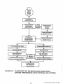
Elements to Plan and Implement a Regional Air Toxics Monitoring Program .....................
2
2- 1
Getting a Monitoring Program Started ....................................................
5
3-1
Key Elements of a Plan for Regional Air Toxics Monitoring Program
...........................
Selecting Monitoring Constituents .......................................................
Key Elements of Network Operation .....................................................
Field Instrumentation Operation and Maintenance ..........................................
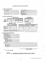
Typical Chain of Custody Form .........................................................
Key Elements of QA/QC for Regional Air Monitoring Programs ..............................
Regional Air Monitoring QA/QC Strategy ................................................
Summarizeand Evaluate Results ........................................................
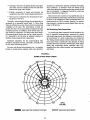
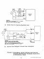
Example Wind Rose Format ............................................................
9
3-2
4-1
4-2
4-3
5-1
5 -2
6-1
6-2
-
iv
10
25
26
27
29
33
34
.
Appendices
Page
A
B
C
D
E
F
...............................
Hazard Index Methodology ............................................................
Air Toxic Monitoring Methods and Equipment ............................................
Bibliography of Air Monitoring Standard Operating Procedures ..............................
65
Excerpt from Technical Assistance Document for Sampling and Analysis of Toxic Organic
Compoundsin Ambient Air ( U S EPA. June 1983. Revised 1990) .............................
71
List of Toxic Air Pollutants for Regional Monitoring Programs
51
55
..............................................
SOPS for Operating VOCS Canister Samples ............................................
91
SOPS for Meteorological Station Operations and Calibration ...............................
169
Data Validation Criteria and Procedures ..................................................
175
Examples of Standard Operating Procedures
U S. EPA Compendium Method TO14 (1988)
G
45
V
89
.
CMA, as part of its ongoing technical education and communication efforts, developed this document as part of
its “Chemicals in the Community:” series. Other documents in this and related series include:
CHEMICALS IN THE COMMUNITY Series includes:
Methods to Evaluate Airborne Chemical Levels, May 1988.
A resource document presents two general approaches for placing emission levels in context: data-base driven
and model driven. Using these two approaches, 8 methods, are described to evaluate the health impact of airborne releases.
Member price $8.00; Non-member price $12.00.
Implementing Regional Air Monitoring Programs, February 1990.
A manual to assist companies establish regional air monitoring programs. This document covers both the
policy issues and the technical details of setting up a regional air monitoring project.
Member price $20.00; Non-member price $40.00.
Understanding Environmental Fate, in preparation.
IMPROVING AIR QUALITY Series includes:
Guidance for Estimating Fugitive Emissions from Equipment, January 1989.
A guidance manual of fugitive emission testing for plants that want to conduct accurate leak rate estimations.
This manual includes the EPA protocol with notations for implementation by the chemical industry.
Member price $20.00; Non-member price $30.00.
Fugitive Emission Workshop Videotapes
These videotapes cover some of the topics plant personnel ask about when setting up a testing program for
equipment leak, detection, and repair (LDAR).
Tape I: Overview
Tape 11: Screening
Tape 111: Bagging
All Three Tapes
Minutes
42
58
38
Member Price
$ 75.00
75.00
75.00
225.00
Non-Member Price
$1 12.50
112.50
112.50
337.50
All tapes are available in ?hand 3/4 inch formats.
POSSEE Software (Plant Organizational Software System for Emissions from Equipment)
POSSEE is a software data entry system for fugitive emissions testing designed exclusively for CMA. POSSEE
can help you set up a testing program, enter data, and develop estimates of the fugitive emissions at your plant.
Member price $150.00; Non-member price $225.00.
A Guide to Estimate Secondary Emissions, In Publication.
A guidance manual for estimation emissions from secondary air sources for SARA 313 reporting.
Member price $40.00; Non-member price $60.00.
PAVE Software, In Development.
To order these documents, please refer to order form on the last page of this publication.
vi
Executive Summary
As responsible members of the communities in which they operate, industries are increasinglymotivated to participate in efforts to measure concentrations of chemicals in the community.
Publics (e.g., community, concerned citizens’ groups, business, and Federal, state, and local regulatory agencies)
have become very aware of the presence of chemicals in the air. These audiences are rightfully demanding credible
information about levels, sources, and effects of chemicals to which they may be exposed. They are expecting
information to:
Determine ambient concentrations of airborne pollutants, commonly known as “air toxics.”
Fill data gaps regarding concentrations of airborne pollutants in the community.
Respond to local, state, or Federal regulatory requirements.
Provide data to evaluate the impacts of airborne chemicals.
Identify contributors of toxic air pollutants in the community. Contributors can include mobile sources, commercial and residential chemical users, and industrial chemical processes. In addition, long-range transport of
air pollutants may contribute chemicals to the community.
Toxic air pollutant monitoring may be needed as part of ozone precursor studies, emergency release evaluations,
and source-receptor relationship studies, including model validations.
)
Regional monitoring programs benefit both the community and industry participants. These programs provide
unique opportunities for cooperative efforts involving industry, regulators, and the community. Ambient data
collected can be of great value to all parties. These data provide a technically sound basis for regulatory decisionmaking and public policy formation.
The purpose of this document is to provide information to those individuals responsible for deciding if and how an
air toxics monitoring program should be undertaken. This document is directed to industry representatives who are
interested in monitoring levels of toxic air pollutants in regions where they operate. It provides a framework for
organizing and participating in regional air monitoring programs. This guidance allows flexibility in tailoring the
program to meet specificlocal needs. It also emphasizesthe cooperativenature of such projects and the steps needed
to involve the public and regulators during the program planning process.
The document also provides specific technical recommendations for conducting an air toxics survey followed by
longer term regional air monitoring. These recommendations are:
Perform air toxics survey monitoring study for preliminary determination of community concentrations as
follows:
- Program duration should be 30 to 90 days.
-
Samples are to be collected for 3 to 24 hours every other day or once in 3 days, depending on the study’s
specific objectives.
- The number of monitoring stations established depends on specific local conditions and program objectives. A minimum of two monitoring stations should be implemented in this type of study.
1
- A portable meteorological station should be used.
vi i
Perform regional air toxic monitoring to establish regional community concentrations as follows:
-
Program duration should be one year or more.
-
Samples are to be collected for 24 hours every sixth day or less.
-
The number of monitoring stations established depends on specific local conditions. For flat or gently
rolling topography with no land/water interface, the network should contain a minimum of three monitoring stations, with one station representing prevailing upwind conditions and the others representing
prevailing downwind stations. The number of monitoring stations can be re-evaluated after one year of
operation.
- The number of meteorological stations established depends on local specific conditions such as topography, the distance between individual monitoring stations, and program objectives. In general, a meteorological station should be located next to each air sampling station. However, this recommendation
could be modified, depending on local specific conditions.
Use the SUMMA passivated canister for sampling of volatile organic compounds (VOCs) and gas
chromatography/mass spectrometry (GC/MS) for subsequent analysis.
Estimated costs for setting up and operating a monitoring network are included in this document. For example,
the estimated first-year cost for installing and operating a regional air toxics monitoring network consisting of four
canister samplers each operating every sixth day at three sites, plus one meteorological station, ranges between
$300,000and $4oo,OOO. Procurement and start-up costs comprise about 25 percent of these costs, with the remainder
allocated to operation, analysis, and data management expenses.
The emphasis of a regional air monitoring program must be on quality to ensure credibility.The quality of the program depends directly on quality management and quality contractors. The data collected during the program must
be impeccable to withstand peer review. It is important that other industries, government agencies, and the public be
involved to gain credibility for the program.
viii
1.0 INTRODUCTION
Before starting a monitoring project, industry must
establish a clear understanding of the overall goal, objectives, and driving forces behind ambient air toxics monitoring. This includes identifyingcommunityconcern and
regulatory requirements.
Ensuring the quality of collected data.
Organizing and reporting monitoring results.
Estimating costs of monitoring programs.
This document has been developed for the Chemical
ManufacturersAssociation (CMA)by NUS Corporation.
Its ultimate objective is to guide planning and implementation of regional air toxics monitoring programs. The
specific objectives of this document are:
0
)
This document is intended to be both a managementand technical-level planning tool which can be useful as a
guide for directing CMA member staff and contractor
activities in regional air toxics monitoring programs.
To provide a basic, yet comprehensive, guide for
planning and implementing regional air toxics
monitoring programs.
0
To allow flexibility in tailoring regional programs
to meet specific local needs.
0
To provide a framework that will ensure consistency
between the various regional programs, which will
allow the development of a useful data base.
0
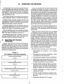
1.1 ORGANIZATION OF THE DOCUMENT
Program elements associated with the planning and
implementation of regional ambient air toxics monitoring are shown in Figure 1-1. This figure includes six key
elements. Each represents a chapter in this document
and is summarized as follows:
Chapter 2.0 (Getting a Monitoring Program
Started) discusses the motivation and philosophy
behind such programs; who should be involved in
the program (public, regulatory agencies, other
industries)and why; and what management factors
should be considered in designing and implementing a regional air toxics monitoring program.
To provide a systematic process for the decision
maker (usually the facility or plant manager
within a region) to ensure the development and
implementation of successful regional air toxics
monitoring programs.
Chapter 3.0 (Developing the Monitoring Plan and
Methodologies) describesthe process for developing monitoring program plans. Key features
include selecting constituents to be monitored;
selecting program duration and frequency;
selecting sampling and analytical methods; defining meteorological program requirements;
designing elements of the network; and selecting
contractors for sampling and analysis.
Those interested in monitoring air toxics levels in communities where they operate will find this document
useful. It primarily addresses how to plan and operate
regional monitoring networks for volatile organic compounds (VOCs). However, monitoring for other constituents, such as metal particulates, are covered in a more
condensed manner.
The document includes specific recommendations for
establishing a regional air toxics monitoring network.
These recommendationscan be modified as needed from
one region to another. Those industries interested in
establishing monitoring networks should consider a joint
program with regulators and the public. These networks
can provide technically sound information to participating sponsors, the public, and regulatory and planning
agencies.
The document provides guidance in the following
areas:
Involving regulators, the public, and other interested parties.
1
Chapter 4.0 (Operating the Network) describes
the process for selecting and training personnel;
procuring equipment; operating and maintaining
field instrumentation; and keeping records.
Chapter 5 .O (Implementing Quality Assurance/
Quality Control) provides guidance for routine
and periodic field, laboratory, and data management QA/QC requirements.
Chapter 6.0 (Managing and Evaluating the Data)
describes the process of storing, reducing, processing, validating, analyzing, interpreting, reporting, and using data.
Structuring the management of a regional air
toxics program.
Chapter 7.0 (EstimatingProgram Costs) provides
estimates for unit costs of equipment and iaboratory analysis as well as estimates of capital and
operating costs, for example, program scenarios.
Developing a monitoring program plan.
Implementing sampling and analysis activities.
1
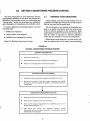
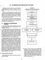
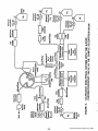
FIGURE 1-1
ELEMENTS TO PLAN AND IMPLEMENT A
REGIONAL AIR TOXICS MONITORING PROGRAM
GETTING A MONITORING
PROGRAM STARTED
(CHAPTER 2.0)
0
DEVELOPING THE MONITORING
PLAN AND METHODS
(CHAPTER 3.0)
Defining your objectives
0
0
0
involving others in the program
0
Establishing a management structure
-D
0
0
0
0
Selecting constituents
Duration and frequency of monitoring
Selecting sampling and analytical
methods
Defining meteorological requirements
Designing the network
Selecting contractors for sampling
and analysis
OPERATING THE NETWORK
(CHAPTER 4.0)
IMPLEMENTING
QUALITY ASSURANCE/ QUALITY CONTROL
(CHAPTER 5.0)
Selecting and training personnel
0
0
0
Defining Q N Q C requirements
Performing routine Q N Q C checks
Implementing periodic Q N Q C checks
Executing laboratory Q N Q C Program
Data management Q N Q C
e-
0
Procuring equipment and supplies
0
Operating and maintaining field
instrumentation
0
Keeping records
1
ESTIMATING PROGRAM COSTS
(CHAPTER 7.0)
MANAGING AND EVALUATING THE DATA
(CHAPTER 6.0)
0
0
0
0
0
1.2
Storing and analyzing the data
Interpreting the results
Re-evaluating the program
Reporting the results
Using the results
+
0
Identifying unit costs of equipment,
supplies, and analysis
Providing example program scenarios
WHY CONDUCT AN AIR TOXICS
MONITORING PROGRAM
Several reasons drive the need for regional air toxics
monitoring programs. They include corporate positions,
regulatory requirements, and public concerns. Communities have become very aware of the presence of
chemicals in the air and are demanding credible information about the levels, sources, and effects of chemicals to
which they may be exposed. Industry is increasingly
motivated to:
a
Fill data gaps regarding concentrations of airborne pollutants in the community.
a
Respond to local, state, or Federal regulatory
requirements.
a
Provide data to evaluate the impacts of airborne
chemicals.
a
Identify contributors of toxic air pollutants in the
community. Contributors can include mobile
^^__I^^^
S U U I LGS,
^^__^_^
1-1
LUIIIIIIGI L l d l
-l---:-..1
LllCllllLill
--A
---:A--L:-l
a l l U I GSlUCIlLlill
chemical users, and industrial chemical processes
and long-range transport of air pollutants.
Determine ambient concentrations of airborne
pollutants, commonly known as “air toxics.”
2
__
__
measures to obtain data from communities. The public,
industry, and regulators can use these data as one input
to evaluatingthe impact that various sourceshave on the
uublic health.
Public awareness of toxic chemical emissions from
industrial and other sources and their effects on public
health and the environment has increased since the
enactment of the Right-to-Know Act under the 1986
Superfund Amendments and Reauthorization Act
(SARA). Federal, state, and local jurisdictions have
enacted regulations or policies that require consideration
of air emissions when issuing permits for both new and
existing sources.
Regional air toxics studies benefit both the public and
industry participants. These efforts provide industry,
regulators, and the public a unique opportunity to work
together to find answers to difficult questions. These
data can provide the technically sound basis for decisionmaking processes.
Regional air monitoring programs can provide information about air quality. These data can address public
and industry concerns and can provide a better understanding of the impact of air toxics emissions. This
knowledge is of particular importance in regions with
large industrial complexes.
This section has provided an overview of the rationale
for conducting an air toxics monitoring program. Other
factors that could affect the decision for conducting an
air toxics monitoring program are driven by regionmecific factors. It is. therefore. imperative for YOU to
carefully review this document A d define your specific
totivations for conducting air toxics monitoring
programs.
Results of well-designed and implemented air monitoring programs provide a “ground truth” for what is
happening in the area or region of interest. In this
respect, such programs can be viewed as proactive
3
L
i
L
GETTING A MONITORING PROGRAM STARTED
2.0
The most critical phase of your regional air monitoring program is planning. In this phase, the direction and
priorities of the program are set, the relationships and
“ground rules” among the Participants are established,
and a foundation of cooperation and credibility is built.
2.1
DEFINING YOUR OBJECTIVES
Clearly identify all of the potential objectives for the
program in the beginning of the project so that the priorities for the study can be agreed upon.
To start a regional air monitoring program, you must
take three steps:
Establish your management structure
The overall goal of any regional air monitoring program is to gather information about the presence and
levels of airborne pollutants in the community. Highquality data are needed even if the results are used only to
infer the effect of exposures to airborne pollutants.
These data are essential for sound risk management.
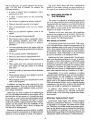
Figure 2-1 illustrates these three key steps.
Within these overall objectives, you will need to consider the characteristics of the region where monitoring
* Define your objectives
Involve others in the program
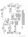
FIGURE 2-1
GETTING A MONITORING PROGRAM STARTED
I
DEFINING YOUR OBJECTIVES
0
W h y are you m o n i t o r i n g ?
0
W h a t questions d o you wish t o answer w i t h this program?
I
W h a t are t h e intended uses o f t h e m o n i t o r i n g data?
I
INVOLVING OTHERS IN THE PROGRAM
I
0
W h o (other industries, regulatory agencies, public) d o you involve?
0
W h y (e.g., end users of final data, users o f detailed data, Q N Q C
participants, m o n i t o r i n g program designers, and program operators)
involve t h e m ?
I
ESTABLISHING A MANAGEMENT STRUCTURE
0
W h a t personnel resources are required and/or available?
W h a t are your b u d g e t resources and constraints?
W h a t are t h e logistical requirements f o r implementing each of t h e
p r o g r a m elements (Figure 1 - l ) ?
0
How should you interact w i t h e q u i p m e n t vendors, outside
laboratories, atid w i t h outside contractors i n impiementing one or
m o r e phases o f t h e p r o g r a m ?
5
The issues posed above and other considerations
specific to your needs will help you make decisions on
the scope of your program and the methods to be used.
will be conducted to set specific objectives for the program. You may want to consider, for example, the
following questions:
In terms of industry and/or population, is this a
growth area or not?
2.2
Is there a natural home for this monitoring
network?
INVOLVING OTHERS IN
THE PROGRAM
The results of a regional air monitoring program will
not be of value unless they are accepted as being valid by
the general public and regulators, as well as the industrial
participants. It is also true that these publics are much
more likely to accept results if they have been actively
included in all stages of the project.
Do you have to organize an industry coalition?
What are the public concerns in the region?
How environmentally active are the citizens
groups?
What are the particular regulatory issues in the
region?
Therefore, at the start, each party with a significant
interest in the program must be involved. This involvement will ensure that the results are useful. Hence, you
must consider the following questions:
Are new regulations being developed?
What factors (such as climate, topography, industrial operating schedules, and public activity
patterns) could affect exposures to airborne
pollutants?
Who should you involve?
All interested parties must be involved. Their objectives, once agreed upon, should be incorporated into the
project planning stages to help create a focused program
effort. Some typical parties include the general public,
governmental bodies, industrial groups, and Chambers
of Commerce. These relationships to the involvement
process are described in the paragraphs below.
Are there particular areas in the region which are
suspected of having high ambient levels of airborne
pollutants?
Do they contain sensitive subpopulations?
Where do these sensitive subpopulationslive?
Identifying who in the “general public’’ should participate in the monitoring program is not easy. In general,
you need to involve those groups or individuals whose
acceptance of the study results would be most credible
among other members of the public. For example, prime
candidates for inclusion are public interest or environmental advocacy groups or neighborhood coalitions in
areas where exposure levels are considered to be high.
What kind of data (e.g, short- or long-term)do you
want?
What studies have been conducted previously in
your region and what gaps remain in the existing
data base?
What is the quality of past data and how defensible
are they?
Responsibility for air toxics regulations or policies
generally resides with Federal, state, or local air pollution
control agencies. To add credibility to your program,
consider involving, or at a minimum, informing key
agency staff in the regional monitoring program area.
Other governmental bodies, such as regional planning
commissions, may also have a stake in the monitoring
results and should be considered for participation.
What technical resources are available to perform
or assist in the program?
What financial resources are required and/or available for this program?
In addition, you may have other objectives for your
monitoring program. These can include permitting for
facility expansion, model validation studies, and emergency release evaluations.
In addition, other industry groups or the local
Chambers of Commerce are potential participants
because results of the monitoring program may impact
their activities.
Other issues you need to address in the beginning are
how the information generated by the program will be
used and who will have access to it. Ground rules must
be set early to avoid future misunderstandings among
project participants. Participants will expect to access
results and, possibly, ongoing operations data. Nonparticipants can also inquire about the availability of and
access to data. However, there is always a danger that
raw data can be misinterpreted.
What does “being involved” mean?
Involvement really begins with defining program
objectives, as discussed in Section 2.1. If no one agrees
on the goals for its program, the results will be of little
use. Therefore, you should consult the program participants on key decisions such as selecting the constituents
to be included in a preliminary survey and/or the the
final monitoring, agreeingon the sampling schedule, and
selecting the number and location of monitoring sites.
Resources for programs are always limited. Available
resources should be concentrated on the highest priority
objectives, so that the quality of results is not diluted.
6
)
“Being involved” means having enough information,
on a timely basis, about the progress, problems, and
results of the program to judge whether or not it is meeting its objectives.
A management committee, composed of representatives of contributing sponsors.
A corporation formed specifically to run the
program (as was done in the Houston Regional
Monitoring Project).
How are participants kept involved?
An outside party, such as a Chamber of Commerce, which could collect and disburse funds,
with management direction coming from a committee of representatives of contributing sponsors.
Involvement is largely a matter of your establishing
relationships and maintaining communications. Once
the participants are identified, make every effort to
maintain continuity of personnel so that working relationships and credibility are established and maintained.
Send participants information regularly and on a timely
basis. Furthermore, in the planning phase and at key
points throughout the project, you should meet with
participants regularly to discuss key issues, review
results, or solve problems encountered. The public at
large and opinion leaders can be kept informed via open
meetings and press releases. In this regard you should
designate a project participant as the program’s communications coordinator.
2.3
1
Typically, final decision-making power regarding
allocation of resources resides with those who are
financing the study. However, as described in Section
2.2, you should closely consult with a broad range of
participants so that study results can be credibly
communicated and be accepted by the various publics.
Funding for the program may come entirely from
industry or from other sponsors, regulatory agencies,
community groups, or environmental trust funds.
Responsibilities for planning and implementing tasks
are outlined in Figure 1-1. These tasks are discussed in
detail in Chapters 3.0-7.0. Once program objectives are
defined and the management structure is established and
operating, your management group must develop a
monitoring program plan. Even after the monitoring
program plan is written, your management team must
continue to follow the plan implementation to ensure
that the program’s objectives are met. Note that all of
the individual items in Figure 1-1 will come into play at
some point during the project.
ESTABLISHING A MANAGEMENT
STRUCTURE
A regional air toxics monitoring program is a complex
undertaking. Depending on program objectives, a program can last from several days to many years. Costs of
the program can be considerable (see Section 7.0). It is
necessary, then, for you to establish a program management structure to make decisions regarding the monitoring program, implement them, and administer funds to
accomplish the program objectives. A number of mechanisms are available to administer the monitoring
program including:
Be aware that if you do not continue to follow the plan
throughout the project, its data and results may not be
defensible.
7
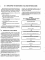
3.0
1
DEVELOPING THE MONITORING PLAN AND METHODOLOGIES
The monitoring plan provides the detailed design for a
regional air toxics monitoring program. It is the design
that sets the boundaries for the program by defining the
elements involved through a well thought-out process.
monitoring and meteorological stations, the use of
models to select monitoring sites, and network design for
dispersion model validation.
Finally, the selection of contractors for performing air
sampling and analysis is discussed in Section 3.7. Also,
the elements associated with such a selection process are
included in this section.
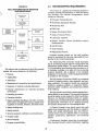
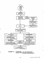
By developing a monitoring plan, you will answer the
following key questions:
What constituents will be monitored?
How many monitoring stations will be involved
and where will they be located?
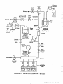
FIGURE 3-1
KEY ELEMENTS OF A REGIONAL AIR TOXICS
MONITORING PROGRAM
What is the sampling duration and frequency and
the program length?
What sampling and analysis methods will be
employed?
SELECT1NG CONSTITUENTS
Section 3.2, Figure 3-2, A p p e n d i c e s A and B
Who and what will be the resource requirements
involved?
Answers to these questions early in the program save
time and money by streamliningthe process, eliminating
unneeded steps, and avoiding pitfalls.
3.1
SELECTING DURATION AND FREQUENCY OF MONITORING
Section 3.3, Table 3-1
OVERVIEW OF PLAN ELEMENTS
SELECTING SAMPLING AND ANALYTICAL METHODS
A good monitoring plan consists of several steps
including those shown in Figure 3-1. A brief discussion
of each of these steps occurs in the following paragraphs.
Section 3.4, Tables 3-2 and 3-3, Appendices C and D
In developing a monitoring plan, first select the constituents to be monitored. Section 3.2 discusses factors to
be considered in developing this list.
Secondly, define the duration and frequency of monitoring to meet specific program needs. Section 3.3 provides
a discussion of this subject. Table 3-1 provides general
guidelines for program length, sampling duration and
frequency by program objectives.
DESIGNING THE NETWORK
Section 3.6
Third, a key element of the monitoring plan is the
selection of sampling and analysis methods most suitable
for your program. This selection is based on the program
objectives, resources, and constraints. Section 3.4 provides a discussion of sampling and analysis methodologies. Details are provided in Appendices C and D.
)
i
In addition to the air monitoring methods, the meteorological monitoring requirements associated with each
air monitoring program are important. A discussion of
these requirements is included in Section 3.5.
Next comes the design of the network which is described in Section 3.6. This section covers the number and
locations of monitoring stations, the siting of air
9
_-
3.2
The Superfund Amendments Reauthorization Act
(SARA) 313 list contains some components that are very
difficult to measure. For some components, new sampling and analytical methods are needed. In fact, for some
pollutants, the monitoring difficulties are cost prohibitive.
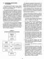
SELECTING CONSTITUENTS
OF INTEREST
Once a decision has been made to conduct a regional
air monitoring program, you have to establish a list of
constituents to be analyzed. Figure 3-2 outlines the
process for selecting constituents.
If the monitoring results for a large number of the
measured constituents are below the detection limits,
you can reduce the list of constituents to be monitored.
Otherwise, one may choose to continue monitoring all
constituents listed in Appendix A.
The starting point is the list of chemicals of concern to
the community. Not aIl airborne pollutants are measurable
using existing techniques. To aid the reader, the lists of
pollutants that are on the U.S. Environmental Protection
Agency @PA) lists of volatile organics quantified in the
Toxic Air Monitoring Stations ( T A M S ) program and the
Urban Toxics Monitoring Program are provided in
Appendix A. These lists include all of the compounds
which EPA considers to be amenable to analysis. EPA
uses this list extensively in its air monitoring programs.
Appendix A also includes the Houston Regional Monitoring (HRM) list of air pollutants. This list includes the
compounds analyzed under the HRM program.
Since the primary goal of the program is to identify
concentrations of air pollutants in the community, the
selected list of constituents for monitoring should reflect
local concerns and issues. To meet this objective, it is
recommended that you evaluate the following:
Community concerns regarding certain types of air
toxics. This should be a key factor in the selection
process of constituents to be monitored.
Air toxics release inventories filed under the
requirements of the “Toxic Chemical Release
Reporting; Community Right-to-Know,” (40CFR
Part 372 subpart D). EPA has computerized these
inventories, and these data are accessible to the
public. Such data will provide information on air
toxics releases to the atmosphere from reporting
industries. You can obtain additional release information from Federal and state agencies. In addition, EPA has information on estimates of air toxic
constituents emitted from mobile sources.
To confirm the presence of the chemicals in Appendix
A in your region, it is recommended that you consider
conducting a short-term air monitoring survey to collect
a limited number of samples and analyze them for all the
constituents included in this appendix. These results will
provide preliminary insight on the presence and magnitude of the detected constituents.
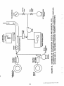
FIGURE 3-2
SELECT1NG MONITORlNG CONSTITUENTS
Air monitoring data available from previous monitoring programs in the monitored region. These
data would identify potential air toxics’ constituents
and their estimated concentrations. Use such data
with caution because changes in demographics may
have occurred after these data were collected. Section 3.8 contains several references on previous
monitoring programs.(’?273)
COMPOUNDS OF
CONCERN TO THE
COMMUNITY
AIR TOXICS
SURVEY RESULTS
AIR TOXICS
RELEASE
INVENTORY
AIR TOXICS
POLICIESAND PROCEDURES
PREVIOUS AIR
MONITORING DATA
I
I
I
I
I
CONSTITUENT RANKING
INDEX (SEE APPENDIX B)
AIR MODELING
SELECTED LIST
OF CONSTITUEXTS
10
Results of air dispersion modeling. Such results
provide information on calculated levels of air
toxics at different locations within the community
relative to their releases.
Lists contained in state and local air toxics policies
and procedures.
Constituents Ranking Index (CRI) values. These
can provide important information for establishing
priorities for air toxics constituents as a part of the
selection process. The ranking process is explained
in Appendix B. The CRI is the ratio of a constituent’s
calculated or measured air concentration to a
health-oriented number derived from animal
experimental data. The derived ratios are used to
rank the constituents as explained in Appendix B.
Other ranking methods are avaiiabie for the
selection of the list of target constituents.
Examples include The Modified Hazardous Air
Pollutant Prioritization System (MHAPPS)(4)and
Source Category Ranking System(5).
)
In most cases, the 24-hour sampling duration is highly
recommended for long-term monitoring for both
organic and inorganic constituents. Use the 8-hour
sampling duration for compliance studies, acute health
effects studies, or preliminary survey studies. For compliance and health studies this duration is used to maintain consistency with the 8-hour TLV values. Sampling
for air toxicity monitoring survey studies is done for
periods of 8 hours to provide more data points during a
short period of time.
Using these factors, together with the results of the air
toxics survey monitoring, can provide you the basis for
determining whether your regional air toxics program
will address all the constituents included in Appendix A,
add more constituents, or reduce the list to fit your specific regional situation. The selected list of constituents
should be specific to each study area.
3.3
Use a 12-hour sampling duration for determining the
effect of daytime and nighttime meteorology on air toxic
concentrations. This sampling duration covers nighttime
thermal inversions.
SELECTING DURATION AND
FREQUENCY OF MONITORING
Apply the 3-hour sampling duration to several objectives. Use it during ozone formation studies, when the
period between 6:oO a.m. to 9:oO a.m. is very critical.
Apply the 3-hour sampling duration to cover meteorological events such as nighttime thermal inversions or
on-shore breezes, or unusual events associated with the
operation of industrial facilities. The 3- to 8-hour sampling periods also are important when sorbent tubes are
used and breakthrough of constituents trapped in the
tubes could occur. Breakthrough could be a factor when
Tenax tubes are used in the sampling program.
Recommendations for sampling duration, frequency,
and length of the monitoring program are summarized in
Table 3-1 by program objectives. Primary program
objectives include air toxics survey monitoring, and
long-term monitoring to establish community concentrations of air toxics. Other program objectives include,
for example, short- or long-term effect studies, compliance studies, or permitting studies.
Actual sampling duration, frequency, and monitoring
program length will depend on your specific project
objectives and on your available project resources. A
representative number of air samples must be collected
during the monitoring program to provide a reasonable
data base. The number of representative samples depends
on many factors. A simple, statistical analysis may not
provide a good basis for determining this number. The
recommendations specified in Table 3-1 are based on the
following factors:
The recommended program lengths in Table 3-1 provide a reasonable data base that can be used in the application under consideration. For most of the program
objectives in Table 3-1, you should obtain a minimum of
30 samples. If the program lasts less than a year, this will
result in an increased sampling frequency.
For model validation study, 24-hour integrated samples are generally suitable. Short-term samples, such as
1-hour averages, can closely track effects of variability in
wind direction. However, these advantages are frequently
offset by the need to deploy more samplers to increase
the likelihood of sampling in the contaminant plume,
and by increased laboratory cost for more samples.
Frequencies usually adopted in monitoring programs for criteria air pollutants involving the use of
time-integrated samplers. A minimum of one
sample every six days is collected to provide random weekday and weekend sampling.
Use of continuous monitoring for program objectives that require short sampling durations.
When the program lasts less than a full year, identify
any ‘‘reasonableworst-case” period for the monitoring
program. This period is characterized by high groundlevel concentrations of air toxic releases from industrial
and nonindustrial sources.
The resource requirements for laboratory analysis
for organic and inorganic compounds.
Quality assurance/quality control requirements
such as collocated field and trip blank samples, and
spike samples.
1
Samples taken over a very short period of time (a few
minutes or so) do not represent average concentrations
of airborne pollutants. High variability could occur over
short periods of time. Samples taken during regional air
monitoring surveys should be averaged over at least one
hour and, preferably, over a longer period of time.
Use air emission release-rate models and atmospheric
dispersion models to identify reasonable, worst-case
exposure conditions (i.e., to quantitatively account for
the above factors). For a worst-case application, limit
the modeling effort to a screening/sensitivity exercise to
obtain “relative” results for a variety of sources and
meteorological scenarios. Consider only those meteorological parameters of greatest significance (e.g., temperature, wind speed, and stability).
You should tailor the general guidance presented in
Table 3-1 to your specific applications.
Cost is a major consideration in selecting the €requency and duration of the sampling program. Overall
11
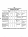
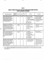
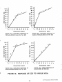
TABLE 3-1
Sampling Duration
Sampling Frequency
Program Length
Program Objectives
1 Hour
3 Hours
8Hours
12Hours 24Hours 5 7 D a y s
30Days
90Days
1 Year
> 1 Year 5 7 Days 30Days
90Days
1 Year
> 1 Year
L
I PRIMARY OBJECTIVES
1
0
Survey Studies
0
-tstauisn
. . . community
c-oncentrations
0
R
Every
0
Oncein
0
R
R
R
Once i n
3days
Once in
6days
Once in
bdays
0
R
0
R
Once in
3days
Once in
6days
Once in
6days
0
R
0
Every
Oncein
other day 3 days
Oncein
6 days
R
0
0
Once in
3days
Once in
6days
Once in
6days
0
0
0
0
Every
Oncein
otherday 3days
Oncein
6days
Oncein
6days
0
0
0
Once in
3days
Once in
6days
0
0
0
Once in
3days
Once in
6days
0
0
0
II OTHER OBJECTIVES
0
Long Term Effects Studies
0
Short Term EffectsStudies
0
Refine Source-Receptor Relationships
0
Compliance Studies
0
0
Model Validation Studies
0
R
Daily(3)
Permitting for Industry Future
Expansion
0
R
Daily(3)
Emergency Release Evaluations
0
0
R
0
(1)
(21
(3’
= Recommended
= Optional
Applicable t o ozone precursor studies
Applicable t o diurnal effects studies
Multiple samples during each day
0
O(1)
R
0
0
0
R
O(21
Daily(3)
0
0
R
operating costs for a program are, in large measure,
directly proportional to the numbers of samplescollected.
Section 7.0 illustrates the effects that the program's
duration and sampling frequency can have on costs.
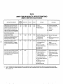
for regional air monitoring programs. Table 3-2 presents
a listing of typical time-integrated monitoring techniques. A brief description of these techniques, the EPA
method number, and the type of compounds detected
are included in Table 3-3. Additional details are included
in Appendix C.
Select sampling periods in a way that will satisfy regulations and public opinion. This kind of scheduling will
help avoid criticism that sample periods do not represent
industrial practices or other activities in the community.
Address the potential problem by adopting a random
schedule with the minimum practical advance notice.
Also, consider collecting more samples than are needed
for the data base, and then decide at a later time, which
samples will be analyzed. (See Section 3.4 for a discussion of sample holding time limitations.)
3.4
U. S. EPA considers canisters for collecting whole-air
samples on a time-integrated basis as the method of
choice, but not the only acceptablemethod, for sampling
volatile organic compounds. It is the recommended
method for regional air monitoring programs. Sorbent
tubes and Tedlar@bagsshould be considered as second
and third choices, respectively, for collecting volatiles on
a time-integrated basis. You should be aware of the limitations associated with these methods. They include a
short holding time from sampling to analysis and a
higher risk of sample losses and contamination.
SELECTING SAMPLING AND
ANALYTICAL METHODS
Near-real-time air toxic monitoring techniques are a
second choice alternative to time-integrated methods.
These techniques can provide reasonably accurate information (in ppbs) on ambient air quality of organic compounds in the gas phase. They also use a combination of
air sampling and a near-real-time analytical analysis
without the use of offsite laboratory facilities. The
analysis is performed with field portable gas chromatograph (GC) systems (see examples in Table 3-2).
Alternative air toxic monitoring techniques for
regional air monitoring programs are classified as
follows:
Time-integrated techniques.
Near-real-time techniques.
Screening-level techniques.
Time-integrated air monitoring methods are applicable when high-quality data are required and the shortterm, temporary variability of concentrations is not
important. In fact, these methods are the most suitable
Limitations of the near-real-timemethods included in
the following:
TABLE 3-2
AN OVERVIEW OF AIR TOXICS MONlTORlNGlSAMPLlNG TECHNIQUES
Technique
Classification
Gas Phase:
I
e
Traps(s0rbentsandcryogenics)and laboratoryanalysis
e
Whole-air samplers (canisters and bags) and laboratory analysis
le
Liquid impingers
Many organic compounds by chemical species
Fraction
ppb ppb
Of a
Historical-integrated
Many organic compounds by chemical species
Historical-integrated
I
I
I
MonitoringISampling
Mode
Compounds Detected
Fraction Of a
ppb to ppb
I
I
I
Detection
Limit
Category of MonitoringlSampling Method
1
Aldehydes, ketones, phosgene, cresollphenols
I
Historical-integrated
b
Particulate Phase:
Gas Phase:
Gas Phase:
0
High-volumesamplers with glass fiber filter. membrane filter or
Teflon filter
pg/m3
lnorganics
Historical-integrated
0
High-volumesamplerswith glass fiber filter and polyurethane
foam'
uglm3
PCBs and other semi-volatile organic species
Historical-integrated
Limited l i s t of organic compounds by chemical species
Historical-integrated
e
Portable field GCanalyzerswith constant-temperatureoven
0
Field GC laboratory
0
Total Hydrocarbon (THC) Analyzers
e
)
ParticulatePhase:
Colorimetric gas detection tubes and monitors
ppb
I
ppb
ppm
Most organics but not by chemical species
Realtime-continuous
ppm
Various organicrand inorganics for a specific chemical
species
Historical-integrated
0
Electrochemical alarm cells
ppm
Various organics fora specific chemical species
Realtime-continuous
e
Portable pumpswith filters
mgIm3
Most inorganic compounds
Historical-integrated
0
Portable pumps with filters 2nd specia! p1u:r
mgld
Semi-vclaile :hemica! species
Historical-integrated
Polyurethane foam (PUF) plug i s designed t o collect semi-volatileorganic gases
0
Tedlar is a registered trademark of E.I. DuPont de Nemours and Company
13
__
ILimited list of organic compoundsby chemtcalspecies IHistorical-integrated
-
I
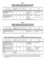
TABLE 3-3
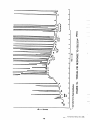
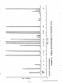
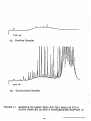
A SUMMARY OF TIME INTEGRATED MONITORING TECHNIQUES FOR ORGANICS AND INORGANICS IN AIR
EPA
Method Number
Technique+
Type of Compounds
Sorption onto Tenax GC Packed Cartridges using low-volume
pump and GUMS Analysis.
TO-1
Volatile, nonpolar organic (e.g., aromatic hydrocarbons,
chlorinated hydrocarbons) having boiling points in the
range of 80" t o 200"C, in gas or vapor phase.
Sorption onto Carbon Molecular Sieve packed cartridge
using low-volume pump and GUMS analyses.
TO-2
Highly volatile, nonpolar organics (e.g., vinyl chloride,
vinylidene chloride, benzene, toluene) having boiling points
in the range of -15" t o + lZO°C, in gas or vapor phase.
Collection of accurately known volume of air into
cryogenically cooled trap in the field and GOFlD or ECD
analyses.
TO-3
Volatile, nonpolar organics having boiling points in the
range of -1 0" to + 200°C. in gas or vapor phase.
Sorption onto polyurethane (PUF) using high-volume
sampler and GUECD analysis.
TO-4
Organochlorinepesticides and PCBs.
Sorption onto Thermosorb/N packed cartridges using
low-volume oumP GUMS analvsis.
TO-7
N-Nitrosodimethylaminein gas phase.
Sorption onto PUF using low-volume or high-volume pump
and high resolution Gas Chromatography/ High Resolution
Mass Spectrometry (HRGUHRMS).
TO-9
Dioxin.
~
Sorption onto PUF using low-volume sampler and Gas-Liquid
Chromatography coupled with ECD.
TO- 10
Organochlorinepesticides.
Sorption onto prepacked silica gel cartridge coated with
acidified dinitrophenylhydrazine (DNPH) using low-volume
pump and High Performance Liquid Chromatography
(HPLC).
TO-11
Formaldehyde.
Sorption t o a combination of quartz filter and a XAD-2 or
PUF cartridge using high-volume sampler and GC with Flame
Ionization (FI) or MS detection or HPLC
TO- 13
Benzo(a)pyrene, [B(a)P] and other polynuclear aromatic
hydrocarbons.
TO-14
Volatile, nonpolar organic (e g , aromatic hydrocarbons)
chlorinated hydrocarbonshaving boiling pointsof -30°C to
about 21 5°C
TO- 12
Non-methaneorganic compounds (NMOC).
ORGANIC COMPOUNDS
- WHOLE AIR SAMPLERS
Whole-air samples are collected in a SUMMA passivated
stainless steel canister and high resolution GC coupled with
mass specific spectrometer (GC MS-SIM or GC-MS-SCAN).
Whole-air samples extracted directly from ambient air and
analyzed using cryogenic preconcentration and direct flame
ionization detector (PDFID), or air samples are collected in a
canister and analyzed by PDFID
Whole-air samples are collected in Tedlar bags and subject
to GUFID or ECD analysis or high-resolution GC compiled
with MS-SIM or MS-SCAN
ORGANIC COMPOUNDS
I
I
Modified TO-3 or
TO- 14
TO-14 or TO-3 Compounds.
- LlOUlD IMPINGERS
-1
Dinitrophenylhydrazine Liquid lmpinger sampling using a
low-volume pump and High Performance Liquid
Chromatography/UVanalysis.
TO-5
Aldehydes and Ketones
Aniline liquid impinger sampling using a low-volume pump
and HPLC analysis.
TO-6
Phosgene.
Sodium HydroxideLiquid lmpinger sampling using a
low-volume pump and HPLC analysis.
TO-8
Cresol/Phenol.
High-volumesampler and Atomic Absorption (AA) or
Inductive Coupled Plasma (ICP).
40 CFR Part 50
Appendix B*
Metals in particulate phase.
PM-10 High Volume sampler and AA or ICP.
40 CFR Part 50
Aaaendix J*
lnhalable metals in particulate phase (up t o 10 microns in
diameter).
High-volumesampler
*Additional details are included in Appendix C
* For sampling methodology only
14
1
Relative and absolute concentrationsof compounds.
The list of chemical species that can be accommodated is shorter than the one handled by a fully
equipped, offsite laboratory.
Relative importance of various compounds in program objectives.
Only an uncomplicated matrix of chemical species
can be analyzed.
Method performance characteristics.
Potential interferences present at the monitoring
site.
As field techniques, these methods lack the ability
to comply with the comprehensive quality assurance/
quality control (QA/QC) procedures used by a certified offsite laboratory.
Time resolution requirements.
Cost restraints.
Screening air monitoring techniques (such as total
hydrocarbon analyzers, colorimetricgas detection tubes,
and industrial hygiene methods) are generally inexpensive, but are only successful for measuring relatively high
detection levels (Le., in the ranges of parts per million for
gaseous contaminants and milligrams per cubic meter
for particulates). Frequently, screening air monitoring
techniques provide near-real-time results in the field.
Alternative survey-level techniques are presented in
Table 3-2. Screening techniques are quite limited in the
number of constituents that can be evaluated concurrently. Hence, these techniques are most effective for air
monitoring near the source to confirm the presence of an
air release and to provide information to support the
development of specifications for a more refined monitoring program. Screening techniques are not recommended for use in regional air monitoring programs.
Base your selection of air monitoring methods and
equipment on a number of factors, including the
following:
Organic and inorganic constituents are monitored by
different methods. Various methods may also be required
for monitoring either organics or inorganics, depending
on the constituentsand their physical/chemical properties.
Whether a compound occurs primarily in the gaseous
phase or is found absorbed to solid particles or aerosols
also affects your choice of monitoring techniques.
Sampling methodologies for PCBs and other semivolatile organic constituents, as well as for inorganics in
the form of particulates, are also included in Table 3-2.
Laboratory analytical techniques must provide for the
positive identification of the components and the accurate and precise measurement of concentrations. This
generally means that the preconcentration and/or storage of air samples are required. Therefore, methods
chosen for time-integrated monitoring usually require a
longer analytical time period, more sophisticated equipment, and more rigorous quality assurance (QA)
procedures.
Physical and chemical properties of compounds.
Table 3 4 presents a comparison of advantages and
TABLE 3-4
COMPARISONS OF REGIONAL AIR MONITORING TECHNIQUES
Time-Integrated
Disadvantages
Advantages
Technique
0
Sampling equipment n o t
complex
0
S t a n d a r d a p p r o a c h used f o r
m o n i t o r i n g air p o l l u t a n t s
~~
Near-Real-ti m e
0
L a b o r a t o r y costs can b e
expensive f o r n i l m e r o u s
samples
0
Short-term temporal
concentration variations n o t
defined
~~
0
Results a v a i l a b l e i m m e d i a t e l y
0
E q u i p m e n t is c o m p l e x
0
Can b e c o s t - e f f e c t i v e f o r h i g h
sampling frequency
0
Number o f sampling
constituents I i m i t e d
0
Provides i n f o r m a t i o n o n
temporal concentration
variations
0
A c c u r a c y c a n b e i m p a i r e d by
interferences
0
S i m p l e t o use
0
H i g h d e t e c t i o n levels
@
inexpensive
M a t r i x interferences a major
problem
15
disadvantages of alternative monitoring techniques. A
list of references and tables which provide additional
guidance on regional air monitoring methodologies is
presented in Appendix C. Tables C-2 through C-10 summarize time-integrated sampling and analysis techniques
for organic and inorganic air pollutants. These methods
are recommended for regional air monitoring.
Primary parameters represent regional dispersion conditions and should be included in all meteorological
monitoring programs. Secondary parameters represent
emission conditions.
Currently, the use of sigma theta in determining
atmospheric stability is an EPA acceptablemethod. EPA
is considering the use of the vertical temperature difference, delta T, in conjunction with net solar radiation to
determineatmospheric stability. Once EPA makes delta T
a part of the method for determining atmospheric stability, it should be integrated in meteorological stations for
regional air monitoring.
Table C-11 in Appendix C includes information on
emerging technologies for regional air monitoring. These
technologies are not recommended for use in regional air
monitoring at this time, but are applicable to some
special purpose studies. This section, along with the data
included in Appendix C, provides useful guidance in the
selection process for regional air monitoring techniques.
3.5
Field equipment used to collect meteorological data
can range in complexity from a very simple analog or
mechanical pulse counter data-logging system, to a
microprocessor-based data logging system. Combine
these approaches for your regional air monitoring program. This recommendation is not expensive and facilitates the convenient collection of meteorological hourlyaveraged data that can be easily processed, using personal computers (PCs). Chart recorders provide a lowcost backup system, if the digital data are not available.
The number of meteorological stations associated with
regional air monitoring programs depends on specific
local conditions such as topography (land/water interface), the distance between individual monitoring stations, and program objectives. A meteorological station
located next to each air sampling station is recommended. However, you could modify this recommendation, depending on your specific local conditions. For
example, one meteorological station could be sufficient
if the following conditions exist: a flat or gently rolling
topography with no air/water interface, no major
obstruction interferences, short distances between stations (a mile or less), and no major emphasis on the
determination of upwind and downwind concentrations.
You should conduct a meteorological survey (i.e.,
short-term data collection) to support air monitoring
network design. Exceptions to this practice would
include areas that have historical, onsite meteorological
data or flat-terrain areas where representative offsite
data are available. The duration of the meteorological
survey should range from 2 to 6 weeks, depending on the
objectives and the design elements of the monitoring
program. In many cases, for planning purposes, you
may use historical, offsite data to estimate seasonal
effects if the air monitoring program is scheduled to last
for more than a few months.
Classes of meteorological monitoring parameters for
regional air monitoring applications include:
Primary parameters including wind direction, wind
speed, sigma theta (Le., the horizontal wind direction standard deviation, which is an indicator of
atmospheric stability), and solar radiation.
Additional recommendations on meteorological
measurements can be obtained from a number of US.
EPA documents.(69 89 9)
Secondary parameters including temperature, precipitation, humidity, and atmospheric pressure.
77
TABLE 3-5
RECOMMENDED SYSTEM ACCURACIES AND RESOLUTIONS
Meteorological Variable
I
I
System Accuracy
+
Measurement Resolution
5% of observed)
Wind Speed
? (0.2 m/sec
Wind Direction
f 5 degrees
Ambient Temperature
f 0.5OC
0.lOC
Dew Point Temperature
? 1.5OC
0.lOC
Precipitation
? 10% of observed
1 f3
Pressure
Source:
U.S. EPA Onsite
Applications(9).
1 degree
0.3 mm
0.5 mb
m b (0.3 kPa)
Meteorological
I
0.1 mlsec
____
f 5 minutes
Time
__
Recommended meteorological monitoring system
accuracies/resolutions and sensor response characteristics are summarized in Tables 3-5 and 3-6, respectively.
DEFlNING METEOROLOGICAL
REQUIREMENTS
I
~
Program
16
Guidance
for
Regulatory
Modeling
~
3.6
DESIGNING THE NETWORK
ing provide locations of calculated high, short-term (up
to %-hour), average concentrations,frequency of occurrence, and locations of maximum, long-term (monthly,
seasonal, and annual), average concentrations.
Number and Location of Monitoring Stations
z
>
Consider the following key factors when selecting the
locations and the number of monitoring stations for
regional air monitoring programs:
The compiled modeling results, together with the
factors listed above, Serve as the
basis to determine the number and locations of monitoring stations.
You should also account for the available resources
and the constraints of the program. Table 3-7 provides
general guidance for selecting the minimum stations for
regional air monitoring and their locations. The actual
number and locations should be determined on a caseby-case basis considering region-specific factors, project
objectives, resources, and budget constraints.
Some of region-specific factors that could increase the
number and locations of your monitoring stations are:
Results of air dispersion modeling for the region
using an atmospheric dispersion model applicable
to the sources and the region under consideration.
Receptor characteristics (population centers, residential communities, sensitive receptors such as
hospitals and schools, and environmental locations, locations of calculated high concentrations
of airborne pollutants).
Environmental characteristics (e.g., meteorology
and topography). Meteorological variables affecting
monitoring network design include wind direction,
wind speed, and atmospheric stability. Use these
parameters to define prevailing wind patterns and
to characterize local dispersion conditions considering source-receptor relationships. Consider
conditions such as nighttime thermal inversions
and downhill drainage flow that are conducive to
high-ground-level concentrations of the toxic
chemicals released from the facility or industrial
sources involved. Topographical effects on plume
dispersion include valley flow and plume dispersion
in complex terrain. Nearby water bodies could
introduce land/water interface and associated
onshore flow (breeze) effects.
Number and locations of sources and their characteristics. Source characteristics include emission
rate, type of source (point, area, volume or line),
type of emissions (fugitive or not), and nearby
structures that could cause wake and plume downwash effects.
These factors can be formulated and incomorated
into a dispersion modeling scheme to calculate *ground
level concentrations of airborne pollutants for the
receptor grid of interest. Results of the dispersion model-
Type of sources involved. Simple sources consist
usually of well-defined emission points and include
several stacks that do not have nearby obstructions.
Complex sources involve large numbers of sources
scattered over a wide area and/or sources that do
not have well-defined emission points. Complex
sources have emissions from roof monitors, vents,
valves, and other components and are defined as
fugitive sources. These sources also include irregular structures that exist near emission locations.
Complex sources will require more monitoring stations than simple sources.
Size of the region involved and community
locations.
Topography coupled with wind flow and land/water
interface, together with wind flow conditions, will
require additional monitoring stations at locations
of anticipated high concentrations.
Areas of high traffic density and locations of major
arteries could require additional monitoring
stations.
Locations of community, commercial, and light
industry activities could require additional monitoring stations.
TABLE 3-6
RECOMMENDED RESPONSE CHARACTERISTICS FOR METEOROLOGICAL
SENSORS
Meteorological Variable
Sensor Specification(s)
I
W i n d Speed
I
Wind Direction
Starting Speed 5 0.5 m/sec; Distance Constant 5 Sm
1
I
Starting Speed 5 0 5 m/sec @ 100 Deflection,
Damping Ratio 0 4 to 0 7; Delay Distance I 5 m
Temperature
Time Constant I1 minute
Dew Point Temperature
Time Constant S 30 minutes; Operating Temperature Range
-3OOC t o + 30OC
Source:
U.S. EPA On-Site Meteorological Program Guidance for
Applications(9).
17
Regulatory Modeling
TABLE 3-7
GUIDANCE FOR SELECTING THE NUMBER AND LOCATIONS OF MONITORING STATIONS FOR
REGIONAL AIR MONITORING PROGRAMS
Minimum
Number of Monitoring
Stations(1)W
Source Type
Location
2
1
a t downwind locations, preferably
in residential areas where high
concentrations are anticipated w i t h
a reasonable frequency of
occurrence
a t upwind location from the sources
preferably in a residential area
3-4 a t downwind locations with similar
characteristics as for simple sources
1-2 a t upwind locationsfrom the
sources, preferably in residential
areas
1.
For sources near topographical features: add t w o stations t o each of the above cases a t
locations of anticipated high concentrations w i t h high frequency of occurrence (plume
impaction at high terrain, location w i t h drainage flow), preferably in residential areas.
2.
For sources near bodies of water: add t w o stations t o each o f the first cases a t locations of
anticipated high concentrations w i t h high frequency of occurrence (plume fumigation
region), preferably in residential areas.
TABLE 3-8
A SUMMARY OF KEY PROBE SITTING CRITERIA FOR AIR MONITORING STATIONS
Criteria
Factor
~~~
~
Vertical spacing
above ground
~~
Horizontal spacing
f r o m obstruction and
obstacles
0
Representative o f the breathing zone and avoiding effects of
obstruction, obstacles, and roadway traffic. Height of probe
intake above ground is in general, 2-3m and 2-1 5m i n the case o f
nearby roadways.
0
A b o u t 1 m or more above the structure where the sampler is
located.
~
0
M i n i m u m horizontal separation from obstructions such as trees
is >2Om from t h e d r i p l i n e and 10m f r o m t h e driplinewhen the
trees act as an obstruction.
Distance from sampler inlet t o an obstacle such as a building
must be at least twice t h e height t h e obstacle protrudes above
t h e sampler.
Unrestricted airflow
0
If a sampler is located o n a roof or other structures, there must
be a minimum o f 2m separation from walls, parapets,
penthouses, etc.
0
There must be sufficient separation between the sampler and a
furnace or incinerator flue. The separation distance depends on
the height and t h e nature of the emissions involved.
0
Unrestricted a i r f l o w must exist i n an arc o f at least 270 degrees
around t h e sampler, and the predominant w i n d direction for t h e
monitoring period must be included i n t h e 270 degree arc.
The sampler must be located far enough away from nearby
roadways t o avoid t h e effect of dust re-entrainment and
vehicular emissions on t h e measured air concentrations.
Spacing from roads
0
Sampler should be placed at a distance o f 5-25m from the edge
o f the nearest traffic lane on the roadway, depending on the
vertical placement of t h e sampler inlet, which could be 2-1 5m
above ground.
18
After you have collected, analyzed, and assessed one
year’s worth of data, you can expand the regional air
monitoring network to accommodate some of the
region-specific factors addressed above.
stations should be located at distances of at least 10times
the heights of any nearby obstructions.
In most cases, it is recommended that meteorological
sensors be placed 10 meters above ground (for wind and
stability data) and instruments for measuring parameters, such as ambient temperature and precipitation,
be placed 2 meters above ground. The use of a portable
meteorological system mounted on a tripod is possible
for certain applications, such as short duration studies.
Siting Air Monitoring and Meteorological Stations
It is likely that one main reason to perform regional air
monitoring is to collect high quality data for use in
decision making. Therefore, the placement of both air
monitoring and meteorological stations is critical to
obtain data that meet data recovery requirements. Currently, for permitting purposes, EPA requires data
recovery rates of 80 percent for air quality data and 90
percent for meteorological data. Any regional air monitoring system established should plan to meet or exceed
these requirements to ensure credibility of the results.
Siting constraints, including power availability, site
access, nearby obstructions, and site security, are integral parts of the monitoring site selection process.
In most monitoring applications, a reliable external
power source is critical. Therefore, if power is unavailable, a candidate site should be excluded from further
consideration.
Placement of air monitoring and meteorological stations must conform to a consistent set of criteria and
guidance. Correct placement ensures data comparability
and compatibility. A detailed set of probe siting criteria
for ambient air monitoring and meteorological programs is given in EPA Ambient Monitoring Guidelines
for Prevention of Signi3cant Deterioration.(8)
Easy access to the site is required to ensure proper program implementation. An access road should be prepared, if required. Or a second candidate site should be
used, if it is more accessible.
Avoid selecting a monitoring site in the vicinity of
nearby obstructions that block air flow, such as buildings
or tall trees; this is particularly important in urban areas.
Key siting factors include the following:
Vertical placement above ground
Site security is an important factor in protecting the
integrity of the program. Sites should have fences and
lights. If possible, equipment should be placed in instrument shelters. In addition, monitoring sites could be
located on residential properties where owners can provide some protection for the equipment.
Horizontal spacing from obstructions and obstacles
Unrestricted air flow
Spacing from roads
Site accessibility
Power availability
Site Preparation Requirements
Site security
Once monitoring sites have been selected, you must
prepare them to accept the monitoring instruments. The
equipment used for VOC and particulate sampling has
its own housing and does not require special instrument
shelters. If you want to monitor for gaseous criteria air
pollutants, (SO,, NO,, CO, 03),
you need a temperaturecontrolled shelter at each site.
Table 3-8 includes a summary of the key criteria associated with these siting factors for air monitoring stations.
You should use the information included in Table 3-8 as
part of the monitoring network design. This will ensure
that the monitoring program provides representativeand
unbiased data. However, site-specific constraints could
make it very difficult for you to meet all siting criteria.
For example, the occurrence of buildings around a candidate monitoring site would make siting very difficult.
Therefore, you should use the information in Table 3-8,
coupled with a balanced evaluation by an experienced air
quality and meteorology specialist. The following
paragraphs discuss key principles you should consider
when siting air monitoring and meteorological stations.
You must prepare platforms for mounting the VOC
samplers and particulate samplers (if required). These
platforms are needed to keep samplers at a proper height
above the ground.
You must also build a tower foundation for the installation of the meteorological station. The size of the foundation can vary, based on the type of tower employed
and the type of soil involved. Meteorological stations
usually are provided with their own housing for the
electronics and data logger and, in general, do not
require additional shelters.
For a monitoring site area with no major obstructions
and obstacles, the air sampler intake should be at the
breathing-zone height of about 2-3 meters above
ground. For a site with nearby roadways, however,
intake placement should take into account the effects of
road dust re-entrainment and vehicu!ar emissions.
An integral part of the site preparation includes the
supply of reliable electricity. In general, the electricity
supply requirements are 1IO-vdt AC and 15-20 amperes.
To ensure a representative exposure, the meteorological
Finally, the monitoring site should be fenced and
19
on dispersion modeling calculations and accurate source
emission data.
lighted at night for security reasons. If it is located on residential property, on the roof of a building, or property
which is otherwise secure, these requirements may not
apply.
Use of Models to Select Monitoring Sites
The locations of air monitoring stations for model
validation applications should be based on local wind
patterns. Air monitoring stations should be placed at the
following strategic locations:
You can also use atmospheric dispersion models to
assist in designing a regional air monitoring program.
Modeling results can identify areas of high concentration,
relative to actual receptor locations. These high- concentration areas, which correspond to actual receptors, are
priority locations for siting air monitoring stations.
Upwind of the facility to characterize background
air concentration levels (based on the expected prevailing wind flow during the monitoring period).
Downwind of the facility at offsite receptor locations which are expected to have the greatest impact
from the releases, considering prevailing wind flows.
However, modeling applications are limited by the
amount, quality, and representativeness of the input
data. Meteorological data are a key input for developing
dispersion or dilution patterns. Unfortunately, the
results of standard dispersion models do not accurately
represent most complex terrain applications (i.e., the
results can be off by greater than a factor of 10). Air dispersion models require emission characterization information as key input. However, the spatial variation of
chemical emissions in complex industrial areas may not
be well-known. Therefore, modeling may not be appropriate, if adequate input data are not available.
Additional locations at complex terrain and coastal
sites associated with pronounced secondary air
flow paths (e.g., downwind of the facility for both
primary daytime and nighttime flow paths).
You should select the above locations prior to initial
monitoring, based on your evaluation of available representative meteorological data.
3.7
The recommended model to evaluate the dispersion of
airborne pollutants for many industrial sources located
in areas of flat or gently rolling topography is the
Industrial Source Complex (ISC) Dispersion Model .(lo)
The use of this model is not difficult, and it is available
for use on a personal computer. Other approved models,
included in the EPA Guidelines f o r Air Quality
Models,(7)are also recommended for use, depending on
the application under consideration.
SELECTING CONTRACTORS FOR
SAMPLING AND ANALYSIS
This document was designed to present information to
develop specifications for obtaining competitive bids
from sampling and analysis contractors. You can identify potential contractors from a review of reference documents, open literature, personal experience, and
professional contacts. By reviewing contractor literature
and publications and by interviewing contractor representatives, you can compile a “short list” of organizations to receive request for proposal on monitoring
activities. You may wish to include a questionnaire
concerning contractor capabilities in this process. Your
request for proposal should specifically describe a scope
of work, schedule, deliverables, methods and procedures
to be used, and other terms and conditions, so that
quotations can be compared on an equal basis. Also, you
should advise the potential contractors of any specific
requirements for status reports and review meetings,
invoicing, and other administrativeitems. As part of the
contractors’ response, you should ask them to identify
and present the qualificationsof any subcontractors that
they propose to use for the project. In general, allow
three to four weeks to permit bidders to present comprehensive proposals.
If sufficient representative data are available, you can
use dispersion modeling to identify the area of maximum, long-term concentration levels at the property
boundary and at actual offsite receptor locations.
Regional air monitoring stations located at the above
locations should provide data to characterizeoffsite concentrations of airborne pollutants.
Designing a Network for Model Validation
Upwind/downwind ambient air monitoring networks
provide concentrations of airborne pollutants at the
point of monitoring, relative to the facility or industrial
complex under consideration. Each air sample collected
is classified as upwind or downwind, based on the wind
conditions for the sampling period. By comparing downwind concentrations to those measured at upwind
points, you can determine the relative contribution of
release from the facility to ambient concentrations of air
Pollutants. This generally accomP1ished subtracting
the upwind concentration (which represents background
conditions compared to the facility contribution) from
the concurrent downwind concentrations. In many
cases, you can directly compare these monitoring results
to concentration increments for a specific source, based
You must consider several key factors when evaluating
contractor capabilities and quotations for ambient air
toxics monitoring. This list is not all inclusive. Develop
your evaluation criteria before contractor bids are
returned so you have an unbiased yardstick to judge the
contractors equitably.
Experience of assigned personnel on similar
projects.
20
)
e
Educational background and training of assigned
personnel.
e
Perceived ability of assigned individuals to work
harmoniously and effectively with the sponsor’s
management and field personnel.
e
Cost, including rate levels and basis, mark-up percentages, and overtime provisions.
e
In-house laboratory capability or established relationship with an outside laboratory.
e
QA/QC policy and practices.
e
Range of methods employed by the laboratory.
e
Mode of communications and management mechanisms between sampling and analyticalpersonnel.
e
Flexibility of approach (e.g., availability of leased
vs. purchased equipment).
e
Contract terms and conditions.
e
Proximity and availability of assigned personnel.
e
Understanding of the objectives and scope of the
program.
e
Laboratory certifications.
18, 1987 through March 18, 1988) and subsequent
updates. Prepared by Radian Corporation, Austin,
Texas 78720.
3. U.S. EPA, January 1988. National Ambient
Volatile Organic Compounds (VOCs) Data Base
Update a n d subsequent updates. E P A
600/3-88/010(A). Contract No. 68-02-4190, prepared by G2 Environmental, Inc.
4. U S . EPA, May 1987. TheModi3ed Hazardous Air
Pollutant Prioritization System (MHAPPs). EPA
Contract No. 68-02-4330, Work Assignment No. 12,
prepared by Radian Corporation.
5 . U.S. EPA, August 1988. Source Category Ranking
System. EPA Contract No. 68-02-4330, Work
Assignment 51, prepared by Radian Corporation.
6. U.S. EPA. February 1983. Quality Assurance
Handbook for Air Pollution Measurements Systems: Volume I K Meteorological Measurements.
EPA-600/4-82-060. Office of Research and
Development. Research Triangle Park, North
Carolina 27711.
Following the evaluation of proposals, you may want
7. U.S. EPA. July 1986. Guidelines on Air Quality
Models (Revised). EPA45/2-78-027R. NTIS PB
86-245248. Office of Air Quality Planning and
Standards. Research Triangle Park, North Carolina
27711.
to conduct further negotiations with one or more bidders.
To simplify management of the project, we recommend
that one contractor be given overall responsibility for the
conduct of sampling and analytical activities, whether or
not the laboratory is a part of this organization or is an
independent laboratory. (In this latter case, the laboratory would be a subcontractor).
3.8
8. U.S. EPA. May 1987. Ambient Monitoring
Guidelinesfor Prevention of SignificantDeterioration
(PSD). EPA-450/4-87/007. Office of Air Quality
Planning and Standards. Research Triangle Park,
North Carolina 27711.
REFERENCES
1. U.S. EPA, December 1988. FY-88 Annual Report
on the Operations and Findings of the Toxic Air
Monitoring Stations (TAMS) and subsequent
updates. Internal Report, Atmospheric Research
and Exposure Assessment Laboratory, Office of
Research and Development, Research Triangle
Park, North Carolina 27711.
9. U.S. EPA. June 1987. On-Site Meteorological
Program Guidancefor Regulatory Modeling Applications. EPA450/4-87-013. Office of Air Quality
Planning and Standards. Research Triangle Park,
North Carolina 27711.
10. U.S. EPA. December 1979. Industrial Source
Complex (ISC)Dispersion Model Users Guide. EPA
Report No. 450/4-79-030. Office of Air Quality
Planning and Standards, Research Triangle Park,
North Carolina 27711.
2. Houston Regional Monitoring Corporation, July
1988. Volatile Indicator Measurement Results from
the Houston Regional Monitoring Network (August
21
OPERATING THE NETWORK
4.0
Good operation of the air monitoring network is critical to highquality data collection and analysis. Therefore, it is imperativethat staff assigned to the program be
well-trained in various phases of network operation.
This will help ensure that the operation and monitoring
plan requirements are met.
In any case, all staff involved with the program should
thoroughly understand the program’s objectives and
specific elements. Staff in management roles should have
prior experience with regional air monitoring programs.
In particular, management personnel should have experience with managing and communicatingwith contractors,
including laboratories; be sensitive to the health riskperception implications of the resulting air monitoring
data; and use skill when relating with agency person-nel,
the media, and the general public. Program managers
must also maintain a high commitment to developing
and implementing quality assurance/quality control programs which meet the needs of their project.
This chapter discusses of the elements associated with
network operations. Figure 4-1outlines these elements.
Properly trained, in-house personnel involved with
the program is an important ingredient for its successful
implementation. Section 4.1 provides a discussionon the
selection and training of project personnel.
Procuring equipment is also an important element in
the program implementation. Section 4.2 provides a discussion of the steps of the procurement process.
For staff, who may be involved in field activities or
other technical roles, prior air monitoring experience is a
valuable asset. Their commitment to QA/QC programs
is also critical.
Once the equipment is procured, installed, and tested,
operating and maintaining the field instrumentation
starts. This subject is discussed in Section 4.3.
Health and safety personnel already may be qualified
to participate in the air monitoring operations. However, those unfamiliar with the low detection levels (parts
per billion or micrograms per cubic meter), which are
typically employed in regional air monitoring, may need
training. Therefore, staff involved with field and other
technical air toxics monitoring projects should be air
quality specialists with relevant ambient air monitoring
experience. Regardless of the individuals’ backgrounds,
they must have a thorough knowledge of, or receive
training in, the equipment and methods to be employed.
Their familiarity with computerized database management techniques would also be beneficial.
Recordkeeping requirements, including various manuals, logs, information sheets, chain-of-custody forms,
and other records, are discussed in Section 4.4.
4.1
SELECTING AND TRAINING
PERSONNEL
In-house staff should be involved with regional air
monitoring programs at various levels. For example,
they may direct and manage the program while implementation is provided by a contractor. Or they may conduct one or more tasks of the program while a contractor
performs the remaining tasks.
Field personnel in particular must be well-trained in:
Understanding the operation of the sampling
equipment.
FIGURE 4-1
Performing the preventive maintenance actions
recommended by the manufacturer.
KEY ELEMENTS OF NETWORK OPERATION
~
_____
SELECTING AND TRAINING PERSONNEL
Conducting timely equipment checks and calibrations.
SECTION4.1
Maintaining the required logs and records to document pertinent field activities. These activities must
be clearly documented for future reference.
PROCURINGEQUIPMENT AND SUPPLIES
Carefully handling collected samples to avoid contamination or loss of materials. This includes documenting, in detail, every sample sent for laboratory
analysis to maintain the correct chain-of-custody.
SECTION4.2
OPERATINGAND MAINTAINING THE FIELD INSTRUMENTATION
Carefully maintaining the program schedule for
sampling and analysis.
SECTION 4.3, FIGURE 4-2
Carefully checking regenerated equipment (canister, traps, plugs, etc.) that are returned by the
laboratory.
RECORDKEEPINGREQUIREMENTS
Consistently collecting QA/QC samples.
SECTION4.4
23
The bids should be evaluated, based on a selected set
of criteria including the following:
Maintaining communications with other project
personnel and management to ensure that they are
kept apprised of any problems and the means of
mitigating them.
Quality and performance of equipment.
Supplier performance and track record.
An integral part of the network operation is communication with the laboratory selected to analyze field
samples. Close communication with the designated contact at the laboratory is critical to ensure that the shipped
samples are received and analyzed on time and that any
technical issues that develop are handled promptly.
Delivery schedule.
Supplier responsiveness.
Support services.
cost.
A number of options are available to train project personnel, who need to supplement their prior training and
experience. These include reviewing documents developed specifically for this program, such as the program
operations plan, and conducting one-on-one meetings
with the operations contractor, laboratory contact, or
other industry personnel who have conducted regional
air monitoring activities. Outside resources, such as U.S.
EPA training courses or workshops, are available.
Publications, such as the references listed in Section 3.8,
are also useful for training purposes. Finally, staff may
obtain vendor literature or attend training sessions
offered by suppliers of air monitoring instruments.
4.2
This evaluation should be made for each piece of air
monitoring equipment that is a part of the program,
including meteorological equipment. Laboratory and
consulting services should also be evaluated.
After you select the successfulvendor, order the equipment and make sure it is delivered to the group that will
install it.
Before using the equipment, you should check it for
proper operation and calibration, if necessary. In addition, it should be inventoried to allow easy tracking. All
supplies should be checked and stored at a location convenient for the field operators. Preparation of a good
inventory management system ensures a mechanism to
replenish supplies on time.
PROCURING EQUIPMENT
AND SUPPLIES
Selecting air monitoring sites and providing access,
site security, 110-volt power, lighting, and platforms (if
needed) are critical elements of the program that should
be completed at the same time as equipment procurement. Typical site preparations include grading, preparing a platform for the instruments, and building a foundation for the meteorological tower.
After a monitoring plan is developed and the program
fully designed, procure equipment and supplies.
Procurement involves developing specifications for
equipment and supplies and making a list of qualified
vendors; evaluating vendors’ bids and selecting the successful vendor@);expediting delivery of equipment and
supplies; performing equipment checks, and preparing
the equipment for field installation.
4.3
Listed below are items that can be used as a basis for
developing vendor specifications:
OPERATING AND MAINTAINING THE
FIELD INSTR UM ENTATION
Field and analytical operations of the air monitoring
program should be conducted in accordance with the
monitoring plan developed for the program (see Chapter
3 .O). Successful implementation of the monitoring plan
requires adequate field staff, program management, and
attention to QA/QC factors. Therefore, program managers should consider applying the operational approach
illustrated in Figure 4-2 to regional air monitoring programs. Developing Standard Operating Procedures
(SOPs) for each type of air monitoring equipment
involved with the program is important. Appendix D
includes a bibliography of Air Monitoring Standard
Operating Procedures. Appendix E includes an excerpt
of QA/QC protocols from the U.S. EPA Technical
Assistance Document for Sampling and Analysis of
Toxic Organic Compounds in Ambient Air. Examples
of SOPs that are pertinent to regional air monitoring
programs are included in Appendix F, These examples
cover the operation and maintenance of the canister
VOCs sampler and meteorological equipment.
Type of equipment and basic source requirements.
Number of pieces necessary for the program.
List of spare parts.
List of necessary supplies.
Equipment instruction manuals and other
documentation.
Warranties.
Delivery time.
Equipment calibration and repair services.
List of clients and number of units sold.
Equipment costs.
Reference methods or other third party specifications which must be met.
24
4.4
FIGURE 4-2
FIELD INSTRUMENTATION OPERATION
RECORDKEEPING REQUIREMENTS
A key factor in a regional air monitoring program is
complete, detailed documentation of field and laboratory activities. The required documentation should
include the following:
AND MAINTENANCE
MONITORING PLAN
(SECTION 3.0)
Personnel Training Records.
SELECTING AND
TRAINING PERSONNEL
(SECTION 4.1)
Monitoring Equipment Manuals.
Monitoring Plan.
Field Logs.
Sample Information Sheets.
PROCEDURES
(APPENDIX D)
OPERATION AND
MAINTENANCE
(SECTION 4.3)
RECORDKEEPING
REQUIREMENTS
(SECTION 4.41
i
I
SAMPLINGIANALYSIS
INSTRUMENTATION
Chain-of-Custody Forms.
Laboratory Logbook
OTHER
TECHNICAL
REFERENCES
Sample Analysis Sheets (including support
documentation).
QA/QC Data.
QC SAMPLINGIANALYSIS
Audit Checklist.
Maintenance Records.
Personnel training records for key staff members
should be maintained by the group responsible for conducting the air monitoring program.
INPUTTO STANDARD
OPERATING PROCEDURES
(SOPS)
(APPENDIX F)
The Monitoring Plan document should encompass
the air monitoring program network configuration and
indeDendent station designs. This record should consist
of atopographical map showing station locations; a set
of drawings, including a site plan with the monitoring
locations identified; and a diagram of the sampling
equipment for each station. Vendor manuals should also
be included in the document.
The subjects that are addressed in the s o p s generally
include, but are not limited to, the following:
0
Purpose.
0
Applicability.
0
Definitions.
0
Manufacturers’ instructions and specifications.
0
Summary of methods, including limitations.
0
General requirements for optional operating
performance.
0
Operating procedures.
0
Operating schedule.
0
Sample handling (handling in the field, communication issues, packaging and storage, sample tracking [chain of custody], shipment, and other issues).
0
Sample holding time.
0
Sample analysis.
0
Routine equipment calibration and maintenance.
The field operator should use a Field Log to maintain
a record of sample numbers, dates deployed, and sampling conditions. The operator should note equipment
condition, sampling problems or equipment failures,
observed weather conditions, and unusual site activities
in the field log.
The field operator should also complete Sample Information Sheets for each sample. The recorded information
should be similar to that required for Field Log Entries.
However, the Sample Information Sheets are samplespecificand are considered the primary sample collection
documentation. The Field Log is a backup document
and presents information on a chronological basis.
A Chain-of-Custody form should travel with each
sample from preparation until the analysis is complete.
Along with sample identification tags, the Chain-ofCustody form is used as a definitive basis to record each
sample’s preparation, deployment, and analytical
history.
Program audits.
0
Record keeping.
0
Program responsibilities.
A Laboratory Notebook should also be maintained.
This document should contain information regarding
25
amounts for each run, as well as any pertinent information, such as sample recovery rates.
Program staff should develop a standard Audit Checklist to standardize and document quarterly audits (see
Section 5.3). The checklist should contain a succinct list
of program requirements. It is a useful resource to indicate compliance status.
the time and date of sample analysis, as well as notes on
the equipment and analytical methods being used. The
laboratory should make copies of this notebook and forward it to the appropriate personnel along with the laboratory results.
Laboratory technicians should routinely use Sample
Analysis Sheets to document analysis results. These
sheets contain a record of detected compounds and
-
FIGURE 4-3
TYPICAL CHAIN OF CUSTODY FORM
Sample Number
Shipper Name
Address
Number
Street
Collector's Name
City
Telephone(
Signature
Date Sampled
State
Time Sampled
Zip
)
Hours
Type of Process Producing Waste
Field Information
Sample Receiver
1.
Name and address of organization recieving sample
2.
Chain of Possessions
1.
2.
3.
Signature
Title
Inclusive Dates
Signature
Title
Inclusive Dates
Signature
Title
Inclusive Dates
26
~
5.0
IMPLEMENTING QUALITY ASSURANCElQUALlTY CONTROL (QNQC)
5.1
Regional air monitoring programs for airborne pollutants consist of complex activities using monitoring equipment and laboratory analysis techniques. This approach
is necessary to accurately quantify concentrations of
airborne pollutants in ambient air. Therefore, it is critical that you ensure and maintain a high-quality program, by implementing the appropriate QA/QC program elements.
DEFINING QUALITY ASSURANCE/
QUALITY CONTROL (QNQC)
REQUlREMENTS
Many people confuse the terms quality assurance and
quality control (QA/QC). Both activities are concerned
with maintaining consistent and verifiable quality in each
element of the program. Strictly speaking, quality control (QC) applies to measures taken, on an ongoing
basis, by personnel involved in producing the primary
output of the program. These actions are taken to maintain performance parameters within acceptable levels.
An example of quality control activity is a routine zero/
span calibration check of a monitoring instrument by the
responsible operating technician.
Figure 5-1 outlines the sections described in this
chapter. Section 5.1 provides an overview of the QA/QC
elements implemented during the operation phase of the
air quality program, Section 5.2 discusses the routine
QA/QC checks, and Section 5.3 addresses periodic
QA/QC checks. Elements of the laboratory QA/QC
program are outlined in Section 5.4. Section 5.5 provides
a discussion of data management QA/QC, including the
type of validity checks to be performed.
Quality assurance, on the other hand, refers to checks
or tests performed by personnel, other than the primary
operators, to verify that the performance parameters
have, in fact, been maintained within acceptable limits.
Examples of quality assurance activitiesare performing a
quarterly audit of monitoring instruments and checking
output data for “out-of-limits” values. In the discussion
which follows, QA/QC is used as a general term to
encompass both QA and QC activities.
FIGURE 5-1
KEY ELEMENTS OF QNQC FOR REGIONAL AIR
MONITORING PROGRAMS
DEFINING Q N Q C REQUIREMENTS
A rigorous QA/QC effort is necessary during the
operation of the regional air monitoring program, to
meet monitoring objectives. Major QA/QC elements
that you should implement during the operational phase
of a regional air monitoring program (see Table 5-1)
include QA/QC management, sample QA/QC, analytical
QA/QC, and data reduction QA/QC.
Section 5.1
.c
PERFORMING ROUTINE Q N Q C CHECKS
Section 5.2
*
QA management involves implementing project-specific administrative procedures to control QA/QC functions. The potential for, and types of, quality problems
vary depending on the activity: sampling, analytical, and
data reduction. Therefore, the individual QA/QC
requirementsmust be developed for each of these activities.
Comprehensive QA/QC recommendationsapplicable to
regional air monitoring programs are available in a
number of documents.
IMPLEMENTING PERIODIC Q N Q C CHECKS
Section 5.3
EXECUTING LABORATORY Q N Q C PROGRAM
Generic air monitoring QA/QC recommendations are
included in the Technical Assistance Document for
Sampling and Analysis of Toxic Organic Compounds in
Ambient Air. (l) Monitoring method-specific QA/QC
recommendations are covered in documents issued by
and NIOSH.(Q Air quality monitorthe U S . EPA(213.4*5)
ing QA/QC recommendations are included in Quality
Assurance Handbookfor Air Pollution Measurements(7)
m d Ambient Monitoring Guidelines for Prevention of
Significant Deterioration (PSD).(8)
Section 5.4
IMPLEMENTING DATA MANAGEMENT Q N Q C CHECKS
Section 5.5
27
The references are included in Section 5.6. Using the
approach illustrated in Table 5-1, you should evaluate
these to identify those appropriate for your programspecific QA/QC requirements.
TABLE 5-1
QNQC ACTIVITIES TO BE SPECIFIED
IN PROGRAM PLAN
Summaries of typical sampling and analysis frequencies
QA/QC requirements, and calibration requirements for
sampling and analysis instrumentation are presented in
Tables 5-2 and 5-3,respectively.
Q N Q C Manaaement
0
QAJQC System Design
0
Document Control
0
Data Evaluation
0
Audit Procedures
0
Corrective Action
0
QAJQC Reportst o Program Management
Training
0
PERFORMING ROUTINE
QNQC CHECKS
5.2
The regional air monitoring program should incorporate the following four-component approach for routine
quality control and assurance checks:
Sample QNQC
0
Instrument Calibration and Maintenance
0
Collection of Routine Quality Control Samples
0
Data Recording
0
Sample Labeling, Preservation,Storage, and Transport
0
Chain-of-Custody Procedures
Use collocated samples for precision checks.
Use blank samples for accuracy checks.
Use analytical standards and equipment calibrations for accuracy checks.
Perform data review for internal consistency.
Analvtical QNQC
0
Method Validation Requirements
0
Quality Control Sample Analysis
0
Data Recording
During each regional air monitoring program, one station with two sets of collocated air samplers should be
used in accordance with Section 4.5 siting criteria. The
goal should be to obtain at least 10 percent of collocated
samples for each monitoring network. The analytical
results from the collocated samplers should be used to
compare and evaluate the integrity of the samples and
the adequacy of laboratory procedures.
Instrument Calibration and Maintenance
Data Reduction QNQC
0
Sample and Analysis Data Files
0
Storage of Raw and Intermediate Data
Preparation and analysis of sample blanks at some
appropriate frequency will ensure program integrity.
Ten percent of the total samples collected is considered
as a minimum amount for sample blanks. After the sam-
Data Validation
TABLE 5-2
TYPICAL SAMPLlNGlANALYSlS FREQUENCIES FOR QC SAMPLES
Type of Sample
Field Blanks
Typical Frequency
Each sample set; at least 10 percent of total
number of samples. Not necessary for VOC
canisters.
Laboratory Blanks
I
Spiked Samples
IEach sample set; weekly.
Daily; at least 10 percent of total number of
samples. Each batch of samples.
I
I
to1located (Para1Iel) Samples
I10 percent of total number of samples.
I
Instrument Calibration Standards
IDaily.
I
Reference Samples
I Weekly.
I
Series (Backup) Samples
IEach sample set.
I
28
\
pling media are prepared for field use, one of each type
of medium should be randomly selected as a field blank.
They should be deployed in the field, but should not be
used to collect ambient samples. Ideally, deploying field
blanks should coincide in time and location with the
collocated sampling. Analysis of the field blanks for
contamination should indicate the acceptability of
sample handling and decontamination operations. This
procedure is not necessary, for VOC canisters. Canisters
must be certified as being clean and free of contamination before sample collection.
FIGURE 5-2
REGIONAL AIR MONITORING QNQC STRATEGY
IMPLEMENT-
IMPLEMENT TECHNICAL
ASSISTANCE DOCUMENT (TAD)
TECHNICAL QA
RECOMENDATIONS FOR AIR
TOXIC MONITORING
METEOROLOGICAL PROGRAM
GUIDANCE. TECHNICAL OA
RECOMMENDATIONS FOR
METEOROLOGICAL MONITORING
-
I
QA CRITERIA IF MORE STRINGENT
Additional routine QA/QC checks are summarized in
Tables 5-2 and 5-3.
5.3
IMPLEMENT SUPPLEMENTALTECHNICAL QA
RECOMMENDATIONSBASED ON OTHER AVAILABLE
REFERENCESAS WARRANTED IF NOTADDRESSEDABOVE
Periodic QA/QC checks should be implemented to
supplement the routine checks. They should include
monthly spiked samples, quarterly audits of program
performance, and quarterly calibration of measurement
and control devices, such as flow controllers, timers, and
meteorological equipment.
You can routinely check the accuracy of sample
analysis by submitting spiked and blank gas samples, as
part of the laboratory analysis package. Spiked samples
should contain a known concentration(s) of some of the
PROGRAM.SPECIFIC AIR
MONITORING QAIQC PROGRAM
Device
IMPLEMENTING PERIODIC
QNQC CHECKS
Parameter Calibrated
Method of Calibration
Comments
Approximate Frequency
SAMPLINGINSTRUMENTATION
measurement device
measurement device
(usually a dry test meter)
Wet or dry test meter or appropriate
flow rate transfer standard
Depends on sampler
(e.g., weekly, monthly,
etc.)
Wet test meter or any appropriate
volume standard.
Depends on sampler
(e.g., weekly, monthly,
etc.)
ANALYTICALINSTRUMENTS
IContinuous monitors(e.g.. IResponse
IUse standard concentrations
FID. PID, FPD, etc.)
instruments
GUMS
IDaily or morefrequently, I Test atmosphere should be
if required
referenced t o a primary standard
(e g., NIST, SRM. or CRM")
Flowlpressure conditions should
duplicate sampling process
I
I
I
Column performance and
responseretention time for
each analvte
Injection of standard using the same
processas for sample injection
Daily or more frequently
if required
Standard composition should be
checkedagainst primary standards if
available
Response and retentiontime
for each analyte
Same as for other chromatographic
instruments
Same as for other
chromatographic
instruments
Same as for other chromatographic
instruments.
lGUMS II
Massspectral resolution and
tuning parameters
*
Must be determined at known
atmospheric pressure and
temperature. Flow rate should be
similar to that used for ramplina.
Daily
(a) Introduction of perfluorocompound directly into MS
(b) Injection of tuning standard
(e.g., bromofluoro-benzene) into
GC
I
I
NIST - National institute Standardization Technology,
SRM -Standard ReferenceMaterial,
CRM -Certified ReferenceMaterial
29
Selection of tuning standards will be
dependent on type of analysisbeing
performed.
I
same compounds that the laboratory is performing
analysis. Blank samples contain only inert compounds
(e.g., nitrogen).
qualified person, who is not directly involved with the
laboratory activities, should validate the data. Elements
of the data validation include evaluation of the quality of
the raw monitoring data against the field and laboratory
QA/QC data and verification of the calculations of
ambient concentrations.
In addition, a quarterly onsite audit is recommended
for the air monitoring program. The audit should consist
of the following:
Meteorological Data Validation
Inspecting sampling stations for general physical
condition and operability.
The validity of raw meteorological data should be
checked using equipment calibration, audit, and performance data. Comprehensivetechnical recommendations
for meteorological data validation are presented in OnSite Meteorological Program Guidance for Regulatory
Modeling Applications.(5) A summary of applicable
meteorological data screening criteria is presented in
Appendix G .
Re-evaluating the source activities.
Evaluating the technical performance and recordkeeping procedures. These are compared to the
specifications in the monitoring plan and appropriate Standard Operating Procedures.
Auditing the air monitoring equipment.
Auditing the meteorological equipment.
Air Monitoring Data Validation
Additional routine QC checks are summarized in
Tables 5-2 and 5-3.
5.4
Similarly, the validity of air monitoring data should
use equipment calibration, audit, and performance data
in a manner similar to that recommended for meteorological data.
EXECUTING LABORATORY
QNQC PROGRAM
A qualified chemist, who is familiar with both the data
validation requirements and the process, should validate
the analytical results. Validation of analytical results for
one sample could take from 15 minutes to more than an
hour, depending on the type of analysis used, the number of air toxic constituents involved, interference, contamination, and other factors.
Laboratory analytical techniques must properly identify the sample components and accurately and precisely
measure concentrations. This generally requires the preconcentration and/or storage of air samples. Therefore,
methods chosen for time-integrated monitoring usually
involve a longer analytical time period, more sophisticated equipment, and more rigorous QA procedures.
Canister sampling includes replicate analyses and duplicate canisters to assess analytical and sampling precision.
Exchanging samples with other laboratories is desirable
to check analytical performance.
Raw air quality data received from portable GC analyzers or other continuous instruments must be checked
for validity. The performance of the analyzer, calibration
information, and QA results should be considered.
Air monitoring data validation efforts should include
statistical analysis, considering collocated sample results
and audit results, to determine data precision and
accuracy. A recommended statistical procedure is presented in Appendix G.
Laboratory QC methods for the regional air monitoring
project should include the following elements: replicates,
spiked samples, control charts, blanks, canisters certification and cleanup, internal standards, zero and span
gases, quality control samples, surrogate samples, calibration standards and devices, and reagent checks.
The laboratory performance in implementing these
elements should be considered as a part of the laboratory
selection process. Specifications for implementation of
these laboratory QC checks are summarized in Tables
5-2 and 5-3. In addition, the analytical methods selected
for program application generally include specific laboratory QA/QC checks.
5.5
5.6
REFERENCES
1. US.EPA. June 1983. Technical Assistance Document for Sampling and Analysis of Toxic Organic
Compounds in Ambient Air and subsequent
updates. EPA-600/4-83-027. NTIS PB83-239020.
Office of Research and Development. Research
Triangle Park, North Carolina 27711.
IMPLEMENTING DATA MANAGEMENT
QNQC CHECKS
2. US. EPA. April 1984. Compendium of Methods
for Determination of Toxic Organic Compounds in
Ambient A i r and subsequent updates.
EPA-500/4-87-Q06. NTIS PB87-168696. Office of
Research and Development. Research Triangle
Park, North Carolina 27711.
Raw monitoring data should be checked for validity,
before they are used as a part of the data base for site
decision-making. These validity checks are an integral
part of the QA/QC program for monitoring activities. A
30
1
6. NIOSH. February 1984. NIOSH Manual of
Analytical Methods. NTIS PB85-179018. National
Institute of Occupational Safety and Health.
Cincinnati, Ohio 45226.
3. U.S. EPA. September 1986. Compendium of
Methods for the Determination of Toxic Organic
Compounds in Ambient Air and subsequent
updates. EPA-600/4-87/006. NTIS BB87-168696.
Office of Research and Development. Research
Triangle Park, North Carolina 27711.
7. U.S. EPA. February 1983. Quality Assurance
Handbook for Air Pollution Measurements.
EPA-600/4-82460. Office of Research and Development. Research Triangle Park, North Carolina
27711.
4. U.S. EPA. June 1988. Compendium of Methodsfor
the Determination of Toxic Organic Compounds in
Ambient Air Second Supplement, (TO-10 through
TO-14), and subsequent updates. EPA Revision
6/88. Office of Research and Development.
Research Triangle Park, North Carolina 27711.
8. U.S. EPA. May 1987. Ambient Monitoring Guidelines for Prevention of Significant Deterioration
(PSD). EPA-450/4-87-007. NTIS PB81-153231.
Office of Air Quality Planning and Standards.
Research Triangle Park, North Carolina 27711.
5. U.S. EPA. June 1987. On-Site Meteorological
Program Guidancefor Regulatory Modeling Applications. EPA450/4-87413. Office of Air Quality
Planning and Standards. Research Triangle Park,
North Carolina 27711.
31
r
i
)
6.0
MANAGING AND EVALUATING THE DATA
FIGURE 6-1
Obtaining and evaluating data from your regional air
monitoring program is your key objective. Steps to
handle, process, and report data are discussed in this
section.
SUMMARIZE AND EVALUATE RESULTS
VALIDATED
AIR/METEOROLOGICAL DATA
Section 6.1 provides guidance to store and summarize
meteorological and air quality data, including the type of
summaries recommended. The format of the database,
however, is not provided in this document. Currently,
CMA is in the process of developing a consistent format
for regional air monitoring data.
GENERATE COMPUTER DATA
BASE FILES
METEOROLOGICAL FILES
AIR MONITORING FILES
After your data is summarized, the interpretationprocess starts. Section 6.2 discusses how to interpret the
results. Section 6.3 addresses the steps associated with
reevaluation of program progress.
SUMMARIZE DATA
6.1
STORING AND SUMMARIZING
THE DATA
STATISTICAL SUMMARIES
The recommended process for managing and evaluating data from a regional air monitoring program is summarized in Figure 6-1.
The first step in the process of summarizing and evaluating the data includes developing a way to handle the
data, usually using a computerized data base. Each
meteorological monitoring station should be equipped
with an automated data processor that provides hourly
average values for each parameter. These data should be
in a digital format that is directly computer-compatible.
Air sampling information and results need to be transcribed from hardcopy records to computer files.
METEOROLOGICAL
SUMMARIES
Monitoring data summaries should be prepared, using
the validated data bases as input. By using these meteorological and air monitoring data summaries, program
managers can readily identify airborne concentrations at
various locations. The main reason to perform regional
air monitoring is to collect high-quality, credible data.
Therefore, data from air monitoring and meteorological
stations must meet data recovery requirements. Currently, for permitting purposes, EPA requires data
recovery rates (total number of valid observations
divided by the total number of possible observations) of
80 percent for air quality data and 90percent for meteorological data. Any regional air monitoring system established should plan to meet or exceed these requirements
to ensure credibility of the results.
AIR MONITORING
SUMMARIES
SUMMARY REPORTS
Listing of hourly averages of all meteorological
parameters for the air sampling periods. This
includes average wind speed, wind direction, wind
vector, ambient temperature, and atmospheric
stability. Recommended units are miles per hour
(mph) for wind speed, degrees relative to north for
wind direction (with this designation indicating the
direction from which the wind is blowing), and
ambient temperatures in OF.
Meteorological Data Summaries
Meteorological data summaries should include at the
least the following:
33
prepared to characterize daytime conditions and nighttime conditions. A summary wind rose (based on all
wind observations during the monitoring period) should
also be developed. A suggested format for wind rose
data is illustrated in Figure 6-2.
Summary wind roses including daytime and nighttime wind roses for complex terrain sites and those
located near large water bodies.
Tabular summaries of means and extremes for
temperature and other meteorological parameters.
Data recovery (of a portion of acceptable data out of
the total database) information should also be presented
to allow for an evaluation of data representativeness. As
mentioned above, EPA currently requires, for permitting purposes, a minimum meteorological data recovery
target of 90 percent.
Data recovery summaries for all parameters (stating percent recovery).
Generally, meteorological listings should generally be
presented on a sequential hourly basis. A 1-hour time
frame is sufficient to account for any short-termtemporal
variability of the data. The presentation of data for
periods less than 1 hour long unduly complicate the data
evaluation process. In addition, these shorter-term listings would be voluminous. For those cases where multiple meteorological stations are used at a single network,
it is desirable to list the data in adjacent columns to
facilitate meteorological data comparisons.
Air Monitoring Data Summaries
Air monitoring data summaries should include a listing of sequential concentrations, measured by station
and monitoring period, that indicates concentrations of
all constituents for which monitoring was conducted.
The listing should indicate method detection limits for
those cases where a constituent is not detected, as well as
upwind/downwind exposure classification (when applicable) and monitoring station operation data (e.g.,
sampling flow rates, station number, and sampling start/
end times).
Statistical summaries for the meteorological data
should be calculated monthly, seasonally, annually, and
for the entire monitoring period.
For sites with diurnal wind patterns (e.g., at complex
terrain or coastal areas), separate wind roses should be
FIGURE 6-2
EXAMPLE WIND ROSE FORMAT
-
WIND DIRECTION FREQUENCY (PERCENT)
34
MEAN WIND SPEED (MIIHR)
observed values, if collected over a one hour period or
less should be compared only to acute health based
criteria, such as an EEGL (Emergency Exposure Guideline Limits) or IDLH (Immediately Dangerous to Life
and Health) or some short-term criteria. Conversely if
potential oncogenic hazard is being evaluated, the
average air value should be the basis for comparison.
This average should include “not detected” values at
some fraction of the detection limit (e.g., detection
limit/2 if the majority of values are detected). In no case
should a significant risk be inferred from values that are
not detected; for example, by using the detection limit
for not detected values, then inferring a significant risk at
the detection limit, but from values which are not
detected. It is recommended that the Constituent
Ranking Index (CRI) approach discussed in Section 3.2
and Appendix B can be used for this comparison. The
CRI value can be considered as the ratio of the air concentration (based on monitoring results) to the appropriate health criterion. If any calculated CRI exceeds unity
(i.e., l), then additional evaluation or assessment is
needed to determine whether a health criterion is
exceeded. CMA, under another project, published a
companion resource document to aid in this evaluation.
This document is entitled, “Chemicals in the Community: Methods to Evaluate Airborne Chemical
Levels.”(2) Copies of this book are available from CMA
publication fulfillment by asking for “Community
Exposure Evaluation” booklet.
It is recommended that you report a concentration of
a constituent that is below method detection limit as ND
(not detected)and to use half the detection limit value for
statistical calculations. This procedure is often done in
the technical community. For example, if the detection
limit for benzene is 1 part per billion (ppb) and laboratory analysis indicates concentrations below method
detection limit, then the value will reported as ND (1.0
ppb). However, for statistical calculations, a value of 0.5
ppb will be used. If more than 30 percent of the values
are below the detection limit, no statistical calculations
should be attempted.
Air concentrations should be expressed in /A g/m3 or
ppb. Raw data used to derive the concentration are also
useful to list in supplemental tables. Such data would
include sampling start and end times, constituent content
in the sample in /A g, volume of air sampled over the
sampling period in m3, and temperature and pressure
conditions during sampling time in O F and mm Hg,
respectively.
Summary tables of constituent-specificconcentrations
measured for each monitoring station should include the
following: minimum and maximum concentrations;
QA/QC concentrations including blanks, duplicates,
and others; detection limits; frequency above and below
detection limits; number of samples; number of occurrences of air concentrations exceeding selected values
(e.g., health and safety criteria, and odor thresholds);
and, when applicable, upwind/downwind concentration
summaries.
Monitoring results can also be used as direct input to
standard risk assessment models. This alternative data
interpretation approach can be used to quantify the total
population risk and maximum individual risk associated
with ambient concentrations of airborne pollutants.
A narrative discussion of sampling results should indicate the problems encountered; the relationship of the
sampling activity to unit operating conditions and meteorological conditions; sampling periods and times; background levels and other air emission sources; and
interferences that may complicate data interpretation.
Also include data recovery for all parameters.
6.3
RE-EVALUATINGTHE PROGRAM
The regional air monitoring program should be
re-evaluated quarterly. The program review should
focus on determining whether program objectives are
being attained. Specifically, among the factors that
should be evaluated during the initial program review
and quarterly, thereafter are the following:
Statisticalsummaries of air monitoring data should be
presented monthly, seasonally, as well as annually, and
for the entire monitoring period. In addition to concentration, means, and extremes, these summaries should
present any other information useful for interpretation,
especially if monitoring results are below analytical
detection limits.
Program accomplishments versus objectives.
Also, present data recovery information to evaluate
data representativeness. A minimum data recovery
target should be 80 percent.
Adequacy of data quality.
6.2
Sample matrix interference problems.
Adequacy of detection levels.
Occurrence of sample contamination.
INTERPRETING THE RESULTS
Acceptable data recovery.
Performance of personnel and equipment.
When interpreting the results of the program, the air
monitoring data should be compared to some constituent-specific health criteria, applicable state/local air
toxics guideline, or ambient air standards. It is important
that the monitoring results be compared to the appropriate health-based criteria. For instance, the maximum
In addition, subsequent annual program reviews
should consider the following factors:
Representativeness of data to characterize typical,
35
Monitoring results
- Meteorological conditions
- Air sampling results
- Quality control
long-term and worst-case, short-term air toxics
conditions in the region.
Changes in population distribution.
Changes in the type or amounts of airborne
pollutants released in your region.
Data interpretation
- Meteorological conditions and representativeness
- Air concentrations vs. health/environmental
criteria
- Program performance (QC and audit results)
Changes in needs of the program sponsors.
Cost-effectiveness of the program.
Changes in public perception of regional air
airborne concentrations and/or potential exposure
opportunities.
The report should provide sufficient details about the
methodologiesemployed in sample collection and analysis,
data management, and QA/QC procedures. Data
summaries should include the type of information discussed under Section 6.1. The availability of raw data
that can be used to arrive at the calculated air concentrations, as discussed in Section 6.1, is critical. Sponsors of
the program should agree on ground rules for making
the raw data available to outside parties.
Emerging regulatory issues.
Availability of improved sampling/analytical
methods and equipment.
Based on the above factors, you can determine
whether program modifications are needed or whether
the monitoring should be discontinued.
6.4
Data should be interpreted, based on the discussion in
Section 6.3. Emphasis should be placed on relating
sources to receptors, by using wind direction data associated with measured concentrations. In addition, risk
assessment calculations should be performed at least
within the framework outlined in Appendix B. Other
methodologiescan be used, depending on the applications
involved and the quality of the experimental animal data.
REPORTING RESULTS AND
CONCLUSIONS
Generally, the public and media are interested in
obtaining results from regional air monitoring programs. Therefore, consider presenting these results during a meeting with representatives from these audiences.
During these meetings, it is imperative to communicate
effectively. CMA, in collaboration with risk communication experts, prepared a resource document entitled,
Risk Communication,Risk Statistics, and Risk Comparisons (CMA, 1988).(3)For your use, the basic CMA
communication strategy includes the following rules:
Volume of data does not result in better interpretation. Instead, valid interpretations require highquality
data that is representative of the ambient concentrations
in the region. Hence, in the summary report, it is important that you provide detailed clearly-stated assumptions
or qualifications related to data interpretation.
Accept and involve the public as a legitimate
partner.
6.5
Plan carefully and evaluate your performance.
Listen to your audience.
OPTIONAL USE OF RESULTS IN
MODEL VALIDATION
Model validation is not easy. However, results of
ambient air measurements can be used to validate
models, provided that the design for the monitoring
program includes considerations for such validation.
Section 3.6 discusses key program design factors to
ensure adequate data quantity and quality for model validation. These factors include (1) the number of monitoring stations considering the topography or nearby
large water bodies; (2)the location of upwind and downwind stations; (3) sampling frequency and duration; (4)
number of samples to be collected; and ( 5 ) the quality of
sampling and meteorological data, including accuracy
and precision.
Be honest, frank, and open to ideas.
Coordinate and collaborate with other credible
sources.
Meet the needs of the media.
Speak clearly and with compassion.
When writing a summary report for the regional air
monitoring program, consider including the following
topics:
Introduction and objectives
Model validation requires the identification of a candidate model and the development of a reasonable
emission inventory. Then monitoring data can be used in
model validation. The American Meteorological
Society’s 1981 document entitled, “‘AirQuality Modeling and the Clean Air Act ’‘(4provides a variety of steps
Executive summary
Monitoring program operations
Network configuration
- Meteorological monitoring
- Air sample collection and analysis
36
that can be used as a measure of the model performance.
These include:
6.6
REFERENCES
1. U.S. EPA, 1978. Guidelines on Air Quality Models
(Revised). EPA45/2-78-027R. NTIS PB86-245248.
Office of Air Quality Planing and Standards.
Research Triangle Park, North Carolina 27711.
The bias (average) of the difference (observed
minus predicted values)
The variance of the difference (noise).
The gross variability (gross error) of the difference.
2. Chemical Manufacturers Association, 1988. Chemicals in the Community: Methods to Evaluate Airborne Chemical Levels. Washington, D.C. 20037.
In addition, measures of correlations can be performed in time, space, or both. Details of the methodologies are outlined in documents produced by the American Meteorological Society(4)and the U.S. EPA.(5)
3. Chemical Manufacturers Association, 1988. Risk
Communication,Risk Statistics, and Risk Comparisons: A Manual for Plant Managers, Washington,
D.C. 20037.
In certain cases, model validation for industrial
sources emitting toxic chemicals can be difficult. This is
because many of the dispersion models currently used
are not capable of handling reactive, volatile organic
compound emissions in the atmosphere. Furthermore,
quantifying the air emissions of the specific pollutant, a
critical input to the dispersion model, can be difficult.
Such factors should be considered as a part of the design
of a model validation program.
4. American Meteorological Society, 1981. Air Quality
Modeling and the CleanAir Act. Recommendations
to EPA on Dispersion Modeling for Regulatory
Applications, Boston, Massachusetts.
5. U.S. EPA. October 1979. ProceduresforEvahating
the Performance of Air Quality Simulation Models.
EPA450/4-79-033. Office of Air Quality Planning
and Standards. Research Triangle Park, North
Carolina 27711.
37
i
".
W
7.0
ESTIMATING PROGRAM COSTS
One of the key questions you will ask is, “How much
does it cost to implement a regional air monitoring program?’, This chapter provides both unit costs and overall
estimated costs for two scenarios of regional air monitoring programs. Cost estimates in this chapter should serve
as a guidance for budgetary purposes only. These estimates
(July 1989) are based on conversations with equipment
manufacturers, suppliers, analytical laboratories,
contractors, and/or the author’s experience implementing various phases of air monitoring programs. Program
costs will vary across the country, depending on the
availability of equipment manufacturers and suppliers,
analytical laboratories, and contractors. Program
managers should get firm quotes to identify the costs
specific to your regional air monitoring program needs.
The cost of the Tedlar@bag sampler includes a
supply of 30 bags at a total cost between $800.00 to
$950.00.
The cost of a polyurethane foam (PUF) sampler
includes brushes, 60 PUF plugs, and 100 fiberglass
filters at a total cost of $300 to $500. Each PUF
calibration kit costs between $100 to $400. When
more than one monitoring station is considered for
the network, only one calibration kit should be
purchased. Hence, a cost adjustment should be
made to exclude this cost of having more than one
calibration kit.
The cost of the high-volume PM-10 sampler
includes brushes and 100 quartz filters at a total
cost of $500 to $700. A PM-10 calibration kit costs
between $100 to $350. As mentioned above, when
more than one sampler is purchased, cost adjustment should be made to exclude the cost of more
than one calibration kit.
Section 7.1 discusses the unit costs for air quality and
meteorological monitoring equipment and supplies as
well as for laboratory analysis. Section 7.2 provides cost
estimates for two program scenarios: one for a 90-day
survey and one for a 1-year study.
7.1
UNIT COSTS OF EQUIPMENT,
SUPPLIES, AND ANALYSES
7.2
Two cases were developed as examples for program
cost scenarios. These can guide the development of other
cost scenarios. However, it should be emphasized that
the cost estimates developed can be used only for budgetary and planning purposes. Refinements should be
made, based on written quotes from equipment manufacturers and suppliers, analytical laboratories, and
contractors.
Cost estimates for equipment, supplies, and laboratory analyses for regional air monitoring programs are
included in Table 7-1. Key assumptions made in developing these estimates are provided as notes to this table.
Monitoring equipment is divided into three groups:
time-integrated air monitoring equipment, near-realtime air monitoring equipment, and meteorological
monitoring equipment. The equipment selected for
inclusion in Table 7-1 is based on the sampling and
analysis methods discussed in Section 3.5 and Appendix
C. When applicable, the EPA-designated sampling and
analysis method is listed in this table.
Case I: Short Duration Survey
In this example, the objective for this short duration
survey is to monitor VOCs in a region that includes several large industrial facilities. This survey could stand
alone or serve as Phase I of a two-phase program. In the
case where the short duration survey is Phase I of a larger
program, the survey purpose is to collect data at several
locations within the community during a season where
meteorological conditions are conducive to high groundlevel concentrations of air pollutants. Then, this survey
will serve as a basis for a long-term monitoring study.
Two types of equipment and supply costs are provided
in Table 7-1. One is for purchasing and the other is for
equipment leasing. The leasing cost is based on recovering the purchase price over a period of 1 year. Table 7-1
also includes cost estimates for laboratory analysis.
Additional assumptions that were made in developing
the costs presented in Table 7-1 are:
1
-
PROGRAM SCENARIO COSTS
The cost of a canister sampler includes three canisters, at total
Of $1,350 to $1,500*Three
canisters are included with each sampler to ensure
continuity of the sampling program, while the
analysis is performed.
The survey study is scheduled to occur over a 90-day
period. Two sampling systems are planned with an
additional system as a collocated unit. In the middle of
the program, the two sampling stations will be relocated.
This wav. data are collected from four sites. The resulting data will be used to provide a preliminary assessment
of the industrial source contributions to ambient air
quality within the region.
< I
The cost of sorption tube samplers (Tenax@and
carbon molecular sieve) includes 30 tubes, at a total
cost of $1,OO0.00 to $1,500.00.
39
TABLE 7-1
RANGES OF UNIT COST ESTIMATES FOR EQUIPMENT AND
SUPPLIES AND LABORATORY ANALYSIS FOR REGIONAL AIR
MONITORING PROGRAMS
cost
EPASampling
and Analysis
Method(6)
Monitoring
Equipment and Supplies(7)
Purchasing
Laboratory
Analysis(@
($/Sample)
Leasing
TIME-INTEGRATED AIR MONIT
I
I
; : :4;
I
450-650
I
450-500(9)
Canister sampler(1)
TO- 14
Tenax sampler(3)
TO- 1
4,000 5,000
350-450
300 -350(11)
Modified TO-3
orTO-14
3,800 4,500
350 - 400
300 - 350(10)
~~
0
Tedlar bag sampler(2)
Carbon molecular
sieve sampler(3)
PCB Particulate
Metals Particulate
0
High-Volume PM-10
sampler(5)
40 CFR
Part50.11
Appendix B
1
NEAR-REAL-TIMEAIR MONITORING
4,500 5,200
'6'ooo -
VOC Gas Phase(15)
I
400-450
I
200-250(14)
1,500 - 1,700
blETEOROLOGICAL MONITORING
Portable system on a tripod
w i t h a chart recorder
Portable system on a tripod
w i t h data logger
Cranked up 10-metertower
system w i t h a chart recorder
Cranked up 10-meter tower
system w i t h data logger
See Note 19
3,800 6,400(16)
300 - 400(17)
Not applicable
See Note 19
7'30010,400(18)
600- 750(17)
Not applicable
4,500 7,300(16)
Assumedno
lease
Not applicable
8,000 1 1,300(18)
Assumed no
lease
Not applicable
Note 19
See Note 19
Includes 3 canisters.
Includes 30 bags.
Includes 30 tubes.
Includes30 plugsand 100 fiberglassfilters.
Includes looquartz filters.
See Appendix C for more details.
Price range is for one unit. Discounts are available for volume purchasing.
Price range is for one sample. Discounts are available for volume analysis.
Method TO-14 analysis, detection limit of about 1ppb and canister regeneration.
Method TO-3 or TO-14 analysis, detection limit of about lppb.
Method TO-1 analysis, detection limit OY about l p p b and tube regeneration.
Method TO-2 analysis, detection limit of about l p p b and tube regeneration.
Method TO-4 analysis, detection limit of about l - 2 ~ g / m 3 .
Atomic absorption/lnductive Coupled Plasma analysis, detection limit of about l - 2 ~ g / m 3 .
Includes portable field GC systems.
System includes wind speed, wind direction, sigma theta and ambient temperature sensors,
lightning protection, spare parts, and calibration kits (upper-range cost).
Cost is based on system described under Note (16) without calibration kits.
Also includes chart recorder as a backup t o the data logger.
Meets requirements specified in Reference 8 in Section 5.6 (EPA-450-/4-87/007) and
Reference 5 in Section 5.6 (EPA-450/4-87-013).
40
Samples will be collected over a period of 24 hours
on every third day.
The following assumptions apply to this cost example:
1
Two air monitoring equipment options could be
used: (1) time-integrated VOCs monitoring using
whole air canister samplers, with subsequent laboratory analysis or (2) near-real-time portable field
GC analyzers.
Fifteen samples will be collected at each of the four
sampling locations for a total of 60 samples.
QA/QC samples for the first option will include 25
samples collected over the 90-day period by the
collocated samplers.
The survey will include a portable meteorological
station.
QA/QC samples for the second option will include
15 canister samples.
The survey will be conducted for a period of 90
days using two sampling systems with an additional
collocated system (for a total of three systems). The
samplers will be moved mid-program, so that a
total of four sampling locations are used.
Site preparation costs (e.g., for electric power and
fencing) are not included.
Table 7-2 provides the cost estimates for a short duration VOCs monitoring survey. The range of estimated
costs for Option I (three time-integrated, whole-air
The monitoring equipment will be leased during the
%day study.
TABLE 7.2
EXAMPLE RANGE OF COST ESTIMATES FOR IMPLEMENTING THE CASE I
SHORT-TERMVOCSAIR MONITORING SURVEY
I
Cost Elements
I
Cost($)*
I
VOCs A i r M o n i t o r i n g
Capital Cost
0
O p t i o n 1 : 3 Time-integrated whole-air canister
samplers
0
O p t i o n 2:3 Near-real-time portable f i e l d GC
analyzers
IMeteorological Monitoring
One p o r t a b l e system o n a t r i p o d w i t h a chart
recorder or a data logger
0
Platforms/lnstrument Shelters - three units
I
I
1,000 - 2,500
1,500
- 2,000
Develop m o n i t o r i n g p l a n
0
Lease e q u i p m e n t and initial check-out
0
_ _ _ _ ~
13,500 - 15,500
500 - 1,000
Spare Parts
Startup Cost
4,500 - 6,000
21,500 - 27,500
~~~
0
Set up e q u i p m e n t i n t h e f i e l d
0
Train in-house personnel
O p t i o n 1 (three time-integrated, whole-air
canister samplers)
Operation Cost
____
-
Supplies a n d samplesshipment
Laboratory analysis
3,500 - 4,000
38,500 - 42,500
4,000 - 5,000
Oneaudit
O p t i o n 2 (three near-real-time portable GC
analyzers)
Data M a n a g e m e n t
and Reporting
Total Cost
Supplies a n d samples shipment
500 - 1,000
Calibration supplies and other expendables
3,000 - 5,000
Laboratory analysis
7,000 - 7,500
0
Data validation
2,000 - 2,500
0
Processing meteorological data
1,500 - 3,500
0
Processing air q u a l i t y d a t a
2,000 - 3,500
0
I n t e r p r e t a t i o n and r e p o r t i n g
4,500 - 6,500
~
Option 1 Monitoring
Option 2 Monitorinq
*Numbers are r o u n d e d t o t h e nearest $500.
41
84,500 - 106,500
58,500
- 78,000
A
The monitoring program will include three fixed monitoring stations. Each will inlcude a VOCs sampler and a
high-volume PM-10 sampler to collect particulate matter
samples for metals analysis. One of the sites will include
a meteorological station and additional collocated VOCs
and PM-10 samplers.
canister samplers) is $84,500 to $106,500. The range of
estimated costs for Option 2 (three near-real-time
portable field GC analyzers) is $58,500 to $78,000. The
main difference between the two options can be attributed to the large laboratory analysis cost under Option 1.
However, using the second option could mean less accurate results, because of some of the limitations of portable field GC analyzers. You should weigh these factors
when selecting one of the two options.
The following assumptions apply to this cost example:
The network will include three fixed stations.
Case II: LongmTerm
Study
The network will operate for one year.
In this example, the purpose is to establish a long-term
regional air monitoring program to measure both VOCs
and metals in a region with several large industrial facilities. The objective of this study is to establish ambient
levels of VOCs and metals at several locations within the
community over a period of a year or more. The data
obtained will be used to evaluate the VOCs and metals
concentrations contributed by the industrial facilities.
The network will include four, time-integrated,
whole-air canister samplers; four time-integrated,
high-volume PM-10 metals samplers; one 10-meter
meteorological station; and auxiliary equipment
and supplies.
The meteorological station will consist of wind
speed, wind direction, sigma theta, and ambient
temperature sensors mounted on a crank-up 10-m
TABLE 7-3
EXAMPLE RANGE OF COST ESTIMATES FOR IMPLEMENTING
CASE I1 LONG-TERM REGIONAL AIR MONITORING PROGRAM FOR
VOCs AND METAL PARTICULATE
Cost Elements
Capital Cost
I
cost
($1
I
JOCAir M o n i t o r i n a
I
I
4 Time-integrated, whole-air canister samplers
I
Metals A i r M o n i t o r i n a
I
~~
0
4 Time-integrated, high-volume PM-10 s a m p l e r s l T 7 , 0 0 0 - 18,000
Vleteorological M o n i t o r i n g
O n e f i x e d system m o u n t e d o n a 10-m cranked u p
t o w e r w i t h a data logger system
Startup Cost
Operation Cost
8,000 - 11,500
Spare Parts
1,000 - 2,000
Platforms/lnstrument Shelters - three units
2,000 - 2,500
0
Develop m o n i t o r i n g plan
0
Procure e q u i p m e n t and i n i t i a l check-out
0
Install e q u i p m e n t i n t h e field
0
Train in-house personnel
0
Supplies and samplesshipment
Laboratory analysis for 232 canister samples and
266 f i l t e r samples
Data M a n a g e m e n t
and Reporting
I
0
I
26,000 - 41,000
1 1,500 - 12,500
I
,73,000 ,99,500
I
Four quarterly audits
I 16,000-20,000 I
Data v a l i d a t i o n
r6sO0
- 9.000 I
Processing meteorological data
0
I
Processing air q u a l i t y d a t a
I n t e r p r e t a t i o n and r e p o r t i n q
42
6,000 - 8,500
8,000 - 13,000
I 16,000- 23,500 I
-
-
~
tower; supporting electronics; data logger; and a
chart recorder.
Table 7-3 provides the cost estimates for a long-term
regional air monitoring study measuring VOCs and
metals particulates. These cost estimates do not include
the short duration survey. If you choose to adopt a twophase program, a short duration survey, and then a longterm fixed monitoring study, the costs must be adjusted
to avoid double counting expenses. In particular, adjustments will be needed for capital and startup costs.
Air samples will be collected once every sixth day at
the three sites for a total of 198 VOCs canister
samples and 198 filter samples.
QA/QC samples will include 34 samples collected
at the collocatedVOCs and particulate metal samplers, add 17 field blanks, and 17 trip blank samples
for particulate metals only. This results in a total of
68 VOC canister samples and 34 filter samples.
Capital costs range from $50,000 to $64,000 dollars.
Startup costs range from $26,000to $41,000. Estimated
annual operating costs as well as data management and
reporting costs range from $237,000 to $286,000. This
results in an estimated first-year total cost range of
$313,000 to $391,000.
The monitoring plan will include a detailed air
dispersion modeling study (reflected in the upper
range startup cost).
No adjustment was made to the cost to account for
discounts on the large volumes of samples to be
analyzed. A cost adjustment could be 10 to 20 percent, depending on the arrangements made with
the laboratory.
These costs could be adjusted to account for changes
in the program. For example, by eliminatingthe PM-10
metal sampling and analysis program, first-year total
costs could be reduced by about $73,000 to $88,000.
Site preparation costs (e.g., for electrical power,
and fencing) are not included.
43
l-
I
"
APPENDIX A
LIST OF TOXIC AIR POLLUTANTS
FOR REGIONAL MONITORING
PROGRAMS
45
APPENDIX A
LIST OF TOXIC AIR POLLUTANTS FOR REGIONAL MONITORING PROGRAMS
This appendix includes a list of airborne pollutants
for regional air monitoring programs. The list consists
of two tables. Table A-1 includes the list of VOCs
quantified in the EPA Toxic Air Monitoring Stations
(TAMS) program and Table A-2 includes the EPA
Urban Air Toxics Monitoring Program Compound
List. Table A-3 includes the list of chemicals analyzed
under the Houston Regional Monitoring (HRM) program. In addition, you may want to consider other airborne pollutants, particularly those on the list identified in the Community Right to Know Act (otherwise,
known as the list in Title 111, Section 313 of the
Superfund Amendments Reauthorization Act
[SARA] of 1986). The lists included in this appendix
contain pollutants for which an analytical method is
readily available. The SARA 313 list contains pollutants for which new sampling and analytical methods
are needed.
TABLE A-2
EPA URBAN AIR TOXICS
MONITORING PROGRAM COMPOUND LIST
Compound Name
1
2
3
4
5
6
7
8
9
10
11
12
13
14
15
16
17
18
19
20
21
22
23
24
25
26
27
28
29
30
31
32
33
34
35
36
37
38
TABLE A-I
LIST OF VOLATILE ORGANICS QUANTIFIED
IN THE EPA TOXIC AIR MONITORING STATIONS
(TAMS) PROGRAM
Compound Name
1
2
3
4
5
6
7
8
9
10
11
12
13
14
15
16
17
18
19
20
21
22
23
24
dichlorodifluoromethane (Freon-12)
methyl chloride
vinyl chloride
trichlorofluoromethane (Freon-11)
dichloromethane
3-chloropropene
1,1,2-trichloro-l,2,2-trifluorethane
(Freon-113)
1,2-dichIoroethane
1,l,l-trichloroethane
benzene
carbon tetrachloride
trichloroethene
toluene
tetrachloroethene
chlorobenzene
ethylbenzene
m-, p-xylene
styrene
o-xy Iene
4-ethyl toluene
1,3,5-trimethyIbenzene
1,2,4-trimethylbenzene
benzyl chloride
1,2,4-trichIorobenzene
47
acetylene
propylene
1,3-butadine
vinyl chloride
chloromethane
chloroethane
bromomethane
methylene chloride
trans-l,2-d ichloroethylene
1,l-dichloroethane
chloroprene
bromochloromethane
chloroform
1,l,l-trichloroethane
carbon tetrachloride
1,2-dichIoroethane
benzene/l,2-dichloroethane
benzene
trichloroethylene
1,2-dichIoropropane
bromodichloromethane
trans-l,3-dichloropropylene
toluene
n-octane
n-octane/trans-l,3-dichloropropylene
cis-l,3-dichloropropylene
1,1,2-trichloroethane
tetrachloroethylene
di bromochloromethane
chlorobenzene
ethylbenzene
m-, p-xylene
styrenelo-xylene
bromoform
1,1,2,2-tetrachIoroethane
m-dichlorobenzene
p-dichlorobenzene
o-dichlorobenzene
TABLE A-3
LIST OF COMPOUNDS INCLUDED IN THE HOUSTON REGIONAL MONITORING
(HRM) PROGRAM FOR AIR TOXICS
CAS#
74-85-1
74-86-2
74-84-0
115-07-1
74-98-6
74-99-7
74-87-3
75-28-5
75-01-4
75-07-0
115-11-7,
106-98-9
106-99-0
106-97-8
74-93-1
624-64-6
74-83-9
463-82-1
107-00-6
590-18-1
75-00-3
67-56-1
75-71-8
563-45-1
78-78-4
123-38-6
67-64-1
75-69-4
109-67-1
75-08-1
503-17-3
64-17-5
563-46-2
109-66-0
78-79-5
N/A
75-05-8
75-35-4
646-04-8
60-29-7
627-20-3
513-35-9
75-09-2
67-63-0
75-83-2
78-84-2
142-29-0
691-37-2
287-92-3
156-60-5
79-29-8
73513-42-5
691-38-3
674-76-0
71-23-8
1
2
3
4
5
6
7
8
9
10
11
12
13
14
15
16
17
18
19
20
21
22
23
24
25
26
27
28
29
30
31
32
33
34
35
36
37
38
39
40
41
42
43
44
45
46
47
48
49
50
51
52
53
54
55
56
Compound Name
CAS#
Compound Name
c-2 voc
ethylene
acetylene
ethane
c-3 voc
propylene
propane
ProPYne
chloromethane
isobutane
vinyl chloride
acetaldehyde
isobutene, l-butene
123-72-8
96-14-0
78-93-3
763-29-1
592-41-6
760-21-4
110-54-3
7642-09-3
67-66-3
625-27-4
4050-45-7
7688-21-3
N/A
96-37-7
107-06-2
108-08-7
71-55-6
590-86-3
71-43-2
27476-50-2
56-23-5
110-82-7
31394-54-4,
565-59-3
110-83-8
107-87-9
78-87-5
589-34-4
71-36-3
110-62-3
96-22-0
79-01-6,
75-27-4
592-76-7
540-84-1
123-91-1
109-79-5
592-78-9
142-82-5
592-77-8
1,3-butadiene
n-butane
methyl mercaptan
trans-2-butene
bromomethane
neopentane
l-butyne
cis-2- butene
chloroethane
methanol
dichlorodifluoromethane
3-methyl-l- butene
lsopentane
propionalydehyde
acetone
trich lorofloromethane
l-pentene
ethyl mercaptan
2-butyne
ethanol
2-methyl-l-butene
n-pentane
isoprene
dimethylsulfide
acetonitrile
1,l-dichloroethylene
trans-2-pentene
diethyl ether
cis-2-pentene
2-methyl-2-butene
methylene chloride
2-propanol
neohexane
is0butyraldehyde
cyclopentene
4-methyl-l-pentene
cyclopentane
trans-l,2-dichoroethylene
2,3-dimethyl butane
is0hexane
cis-4-methyl-2-pentene
Trans-4-methyl-2-pentene
l-propanol
107-39-1
108-87-2
10061-01-5
107-40-4
108-10-1
592-13-2
110-75-8
10061-02-6
79-00-5
565-75-3
554-14-3
108-88-3
616-44-4
591-49-1
124-48-1
N/A
48
57
58
59
60
61
62
63
64
65
66
67
68
69
70
71
72
73
74
75
76
77
78
79
80
81
82
83
84
85
86
87
88
89
90
91
92
93
94
95
96
97
98
99
100
101
102
103
104
105
106
107
108
109
110
111
butyraldehyde
3-methylpentane
butanone
2-methyl-l-pentene
l-hexene
2-ethyl-l-butene
n-hexane
cis-3- hexene
chloroform
2-methyl-2-pentene
trans-2-hexene
cis-2- hexene
c-3-methyl-2-pentene
methylcyclopentane
1,2-dichIoroethane
2,4-dimethylpentane
1,l,l-trichloroethane
isovaleraldehyde
benzene
methylcyclopentene
carbon tetrachloride
cyclohexane
isoheptane, 2,3-dimethylpentane
cyclohexane
2-pentanone
1,2-dichIoropropane
3-methylhexane
l-butanol
valeraldehyde
3-pentanone
trichloroethylene bromodichloromethane
1-heptene
2,2,4-trimethylpentane
1,4-dioxane
Butyl Mercaptan
3-heptene
n-heptane
2- heptene
bichloromethyl ether
2,4,4-trimethyl-l-pentene
methylcyclohexane
cis-l,3-dichloropropene
2,3,4-trimethyl-2-pentene
methylisobutylketone
2,5-d imethylhexane
2-chloroethyl vinyl ether
+
-
trans-1,3-dichloropropene
1,1,2-trichIoroethane
2,3,4-trimethylpentane
2-methylthiophene
toluene
3-methylthiophene
l-methylcyclohexene
dibromochloromethane
3,5,5-trimethyl hexene
-
>.J
)
TABLE A-3 (Cont.)
LIST OF COMPOUNDS INCLUDED IN THE HOUSTON REGIONAL MONITORING
(HRM) PROGRAM FOR AIR TOXICS
CAS#
589-81-1
66-25-1
110-01-0
3522-94-9
111-66-0
127-18-4
111-65-9
7642-04-8
541-31-1
108-90-7
100-41-4
106-42-3,
108-3-3
100-42-5
95-47-6
79-34-5,
75-25-2
124-11-8
2198-23-4
638-02-4
111-84-2
98-82-8
80-56-8
95-49-8
108-41-8
106-43-4
103-65-1
620-14-4
622-96-8
111-44-4
108-67-8
611-14-3
127-91-3
98-06-6
95-63-6
541-73-1
112
113
114
115
116
117
118
119
120
121
122
123
124
125
126
127
128
129
130
131
132
133
134
135
136
137
138
139
140
141
142
143
144
145
Compound Name
3-methyl heptane
hexanal
tetrahydrothiophene
2,2,5-trimethylhexane
1-octene
tetrachloroethylene
n-octane
cis-2-octene
isopentyl mercaptan
chlorobenzene
ethylbenzene
p-xylene m-xylene
CAS#
872-05-9
106-46-7
538-93-2
124-18-5
526-73-8
95-50-1
99-87-6
496-11-7
95-13-6
138-86-3
141-93-5
104-51-8
105-05-5
821-95-4
1120-21-4
91-20-3
75-34-3
74-82-8
100-52-7
107-13-1
156-59-2
108-94-1
106-93-4
110-02-1
564-02-3
126-99-8
67-72-1
74-88-4
75-56-9
593-60-2
1634-04-4
98-87-3
100-44-7
75-21-8
87-61-6
120-82-1
+
styrene
o-xylene
1,1,2,2-tetrachloroethane +
bromoform
1-nonene
4-nonene
2,5-dimethylthiophene
n-nonane
isopropylbenzene
a-pinene
o-chlorotoluene
m-chlorotoluene
p-chlorotoluene
n propyIbenzene
m-ethyltoluene
p.-ethyltoluene
dichloroethyl ether
1,3,5-tri methylbenzene
o-ethyltoluene
b-pinene
t- butylbenzene
1,2,4-trimethyI benzene
m-dichlorobenzene
-
146
147
148
149
150
151
152
153
154
155
156
157
158
159
160
161
162
163
164
165
166
167
168
169
170
171
172
173
174
175
176
177
178
179
180
181
Compound Name
1-decene
p-dichlorobenzene
isobutylbenzene
n-decane
1,2,3-trimethyI benzene
o-d ichlorobenzene
p-isopropyltoluene
indan
Indene
limonene
m-diethylbenzene
n-butyl benzene
p-d iethylbenzene
1-undecene
n-undecane
naphthalene
1,l-dichloroethane
methane
benzaldehyde
acrylonitrile
cis-l,2-dichloroethylene
cyclohexanone
1,2-dibromoethane
thiophene
2,2,3-trimethylpentane
chloroprene
hexachloro Ethane
methyl Iodide
propylene Oxide
vinyl bromide
methy-t-butyl ether
benzal chloride*
benzyl chloride*
ethylene oxide*
1,2,3-trichIorobenzene*
1,2,4-trichIorobenzene*
*These compounds may be more difficult to analyze. Validation cannot be assured at this time.
49
APPENDIX B
HAZARD INDEX METHODOLOGY
51
-.
3
APPENDIX B
HAZARD INDEX METHODOLOGY
This appendix outlines methods for ranking and selecting constituents in the regional air monitoring program.
This ranking procedure is designed to help the user determine which constituents, from a large list of constituents,
to include in the regional air monitoring program.
Generally, the reader must select compounds before
determining what equipment and analytical methods are
used during the regional air monitoring study.
Example 1:
The RfD value4 for lead is: 1.5 cc g/m3. Assume the
calculated annual average lead concentration in the
community, as determined from dispersion modeling, is
0.2 p g/m3. Then the CRI for lead is:
CRI (lead) =
The process detailed in this appendix involves calculating a Constituent Ranking Index (CRI) for each constituent included in Appendix A. The CRI index uses the
expected annual average concentration for a compound
(e.g. from air dispersion/modeling or monitoring) and
compares these expected levels to some criteria that
estimates the potential impact on human health. The
human health criteria used in the ranking process should
be widely available and should reflect an appropriate
measure of potential impact. Among the various
references used to obtain health values are:
Annual Concentration - 0.2
- 1.5 =0.13
RfD
Example 2:
The RfD value for mercury is 0.5 p g/m3. Assume the
calculated annual average mercury concentration on the
community, as determined from dispersion modeling, is
0.1 P g/m3. Then the CRI for mercury is:
CRI (mercury) =
The EPA's Integrated Risk Information System
(IRIS), which is EPA's database for health risk
assessment values. This database is accessible via
computer.
Annual Concentration - 0
.1
- 0.5 =0.2
RfD
Calculating the CRI for Carcinogens.
National Library of Medicine Network, specific
databases such as TOXLINE@, TOXNET@,
Hazardous Substance Data Base (HSDB). This
network is available through Dialogue@and can be
accessed via computer.
The U.S. EPA Health Effects Assessment Summary
Tables, First Quarter FY 89 and updates.
The following are examples for calculating the CRI
for carcinogens. These examples use calculated annual
concentrations derived by a dispersion model.
Example 3:
The reference value (RsD X100) for dichloromethane
is 200 p g/m3. Assume the calculated annual average
dichloromethane concentration in the community, as
determined from dispersion modeling, is 4 p g/m3.
Then the CRI for dichloromethane is:
Please note that not all of these databases are peerreviewed. Therefore, readers should search and review
original studies and individual sources.
The health oriented levels shown in the examples that
follow are based on the assumption of chronic exposure
to an individual contaminant. In the following examples
RfD's1 @PA reference doses) will be used for noncarcinogens, and a multiple of the inhalation RsD2
and/or NOEL3 will be used for compounds that are
animal carcinogens. These types of calculations can
include all constituents under consideration.
Concentration
CRI (dichloromethane) = reference value -
4
200
= .02
Calculating CRI for Non-Carcinogens
Assuming Chronic Exposure
'The RfD (inhalation) is a benchmark dose derived from the NOAEL (NoObserved-Adverse-Effect-Level) by consistent application of order of
magnitude uncertainty factors. If an inhalation RfD is not available, it can be
calculated as lO"/unit risk number p g/m3.
The following examples illustrate calculationsof CRIs
for non-carcinogens. These examples use calculated
annual concentrations derived by a dispersion model.
?he RsD is the dose corresponding to a lod upperbound on risk.
0
3Another measure which has been used is the ED,, value, the estimated dose
correspondingto a 10% tumor incidencein animals.
TOXLINE, TOXNET, and DIALOGUE are registered trademarks of the National
Library of Medicine.
53
Example 4:
Conclusion
The reference value (RsD X100) for trichloroethylene
is 60 P g/m3. Assume the calculated annual average trichloroethylene concentration in the community, as
determined from dispersion modeling, is 10 p g/m3.
Then the CRI for trichloroethylene is:
Once the CRI calculations are completed, the sets of
CRIs for carcinogens and non-carcinogens are ranked
from highest to lowest. The resulting prioritized list
should blend carcinogens and non-carcinogens in the
ranking. To achieve this blending, it is recommended
that for ratios based upon the:
CRI (trichloroethylene) =
Concentration
reference value
-
RsD, the RsD should be multiplied by 100
(corresponding to lo4 upperbound estimate of risk).
NOEL, an appropriate fraction of a NOEL must be
evaluated to appropriately compare compounds. If
NOEL’S are consistently used for all compounds, the
fraction is immaterial since the relative comparison
will be valid. However, if the reader mixes health
criteria, a NOELAM) is recommended to be consistent
with the RfD. For direct acting genotoxic carcinogens
NOEL/1000 has also been recommended.
10
60
Example 5
The reference value (NOEL/100) for carbon
tetrochloride is 60 P g/m3. Assume the calculated
annual averge carbon tetrachloride concentration in the
community, as determined from dispersion modeling, is
10 P g/m3. Then the CRI for carbon tetrachloride is:
Using the examples above for non-carcinogens the
CRI for lead is less than the CRI for mercury. Using the
examples for carcinogens the CRIs for trichloroethylene
and carbon tetrachloride are greater than the CRI for
dichloromethane. After this process, the reader can
evaluate the project’s priorities and select the list of
constitutents for the community air toxics monitoring.
CRI (carbon tetrachloride) =
Concentration - 10
reference value =
60
4Valueused is NAAQS.
54
APPENDIX C
REGIONAL AIR MONITORING METHODS AND EQUIPMENT
i
I
55
NOMENCLATURE USED IN THIS APPENDIX
Gas Chromatograph
Flame Ionization Detector
Photoionization Detector
Electron Capture Detector
Flame Photometric Detector
Mass Spectroscopy
High Resolution Gas
Chromatography
High Resolution Mass Spectroscopy
HRMS
GC-MS-SIM Gas Chromatography-Mass
Spectroscopy-Selected Ion
Monitoring
GC-MS-SCAN Gas Chromatography-Mass
Spectroscopy-full SCAN mode
Preconcentration and Direct Flame
PDFID
Ionization Detector
High Performance Liquid
H PLC
Chromatography
Atomic Absorption
AA
Inductive Coupled Plasma
ICP
Fourier Transformllnfra Red
FTllR
High Volume
Hi Vol
Glass Fiber Filter
G FF
Graphite Furnace At om ization
GFA
Mixed Cellulose Ester Filter
MCEF
(Membrane Filter)
Ion
Selective Electrode
ISE
Flame Ionization
FI
Dinitrophenylhydrazine
DNPH
Ion Chromatography
IC
GC
FID
PID
ECD
FPD
MS
HRGC
56
APPENDIX C
REGIONAL AIR MONITORING METHODS AND EQUIPMENT
TABLE C-1
LIST OF AIR TOXIC MONITORING REFERENCES
1. U.S. EPA. June 1983. Technical Assistance Document for Sampling and Analysis of Toxic Organic
Compounds in Ambient Air and Subsequent Updates. EPA-60014-83-027. NTlS PB83-239020. Office of
Research and Development. Research Triangle Park, North Carolina 27711.
2. U.S. EPA. April 1984. Compendium of Methods for the Determination of Toxic Organic Compounds in
Ambient Air and Subsequent Updates. EPA 60014-84-041.Office of Research and Development. Research
Triangle Park, North Carolina 27711.
3. U.S. EPA. September 1986. Compendium of Methods for the Determination of Toxic Organic Compounds in
Ambient Air and Subsequent Updates. EPA 60014-87-006.NTlS PB87-168696. Office of Research and Development. Research Triangle Park, North Carolina 27711.
4. U.S. EPA. June 1988. Compendium of Methods for the Determination of Toxic Organic Compounds in
Ambient Air. Second Supplement, TO-10 through TO-14) and Subsequent Updates. EPA Revised June 1988,
Office of Research and Development, Research Triangle Park, North Carolina 27711.
1
5. U.S. EPA. 1977. Quality Assurance Handbook for Air Pollution Measurement Systems. EPA-60014-77-027a,
Volume II, Section 2.2-High Volume TSP Samplers, Section 2.11-High Volume PM-10 Samplers. Quality
Assurance Division, Environmental Monitoring Systems Laboratory, Research Triangle Park, North Carolina
27711.
6. NIOSH. February 1984. NIOSH Manual of Analytical Methods. NTlS PB85-179018. National Institute for
Occupational Safety and Health. Cincinnati, Ohio 45226.
7. U.S. EPA. September 1983. Characterization of Hazardous Waste Sites-A Methods Manual: Volume 11,
Available Sampling Methods. EPA 60014-83-040.NTlS PB84-126929. Office of Solid Waste. Washington, D.C.
20460.
8. U.S. EPA. September 1983. Characterization of Hazardous Waste Sites-A Methods Manual: Volume 111,
Available Laboratory Analytical Methods. EPA 60014-83-040. NTlS PB84-126929. Off ice of Solid Waste.
Washington, D.C. 20460.
9. U.S. EPA. 1986. Test Methods for Evaluating Solid Waste.3rd Edition. EPA SW-846. GPO No. 955-001-00000-1.
Office of Solid Waste. Washington, D.C. 20460.
10. ASTM. 1982. Toxic Materials in the Atmosphere. ASTM, STP 786. Philadelphia, Pennsylvania 19103.
11. ASTM. 1980. Sampling and Analysis of Toxic Organics in the Atmosphere. ASTM, STP 721. Philadelphia,
Pennsylvania 19103.
12. ASTM. 1974. lnstrumentation for Monitoring Air Quality. ASTM, SP 555. Philadelphia, Pennsylvania 19103.
13. APHA. 1977. Methods of Airsampling and Analysis. American Public Health Association. Washington, D.C.
20005.
14. ACGIH. 1983. Air Sampling Instruments for Evaluation of Atmospheric Contaminants. American Conference of Governmental Industrial Hygienists. Cincinnati, Ohio 45211.
57
TABLE C-2
SUMMARY OF SAMPLING AND ANALYTICAL METHODS FOR TIME-INTEGRATED
AMBIENT MONITORING: VOLATILE OPRGANICS
Sampling and Analysis Approach
CRY OGENlC PRECONCENTRATlON/GUFlD/EC-Known volume of air is collected accurately onto a
cryogenically cooled trap. Carrier gas transfers the
condensed sample t o a GC column. Adsorbed
compounds are eluted from the GCcolumn and
measured by FID or EC detectors.
-
Method
)esignatior
TO-3
Detection Limit
~
I
Accuracy(')
Precision(2)
0.1 ppbv
(100 ml sample)
D
~~
CARBON MOLECULARSIEVEADSORPTION AND
G/MS or GUFID-Selected volatile organic
compounds are captured on carbon molecular
sieve adsorbents Compounds are thermally
desorbed and analyzed by GUMS techniques.
TO-2
TENAX GCADSORPTIONAND GUMS OR GUFID-Ambient air i s drawn through organic polymer
sorbent where certain compounds are trapped
The cartridge i s transferred t o the laboratory for
analysis Using GUMS or GUFID
TO- 1
SUMMA PASSIVATEDCANISTER AND GUFlDlECD
TO-14
Collects wide variety of volatile
organic compounds
Standard procedures are available
Contaminantscommon to
adsorbent materials are avoided
Lowblanks
~
1 - 200 pptv
(20 ml sample)
70 95%
(biased low)
t 10.40%
I
Advantages
~
Disadvantages
0
0
Moisture levels in air can cause
freezing problems
Difficult t o use in field
Expensive
~~
Trace levels of volatile organic
compounds are collected and
concentrated on sorbent material
Atmospheric moisture not collected
0
Some trace levels of organic species
are difficult t o recover from the
sorbent
~
OR GUMS--Whole air samplesare collected in an
evacuated stainless steel canister VOCs are
concentrated in the laboratory w i t h cryogen trap
VOCs are revolatilized, separated on a GC column,
and passedt o one or more detectors for
identification and quantitation
(1)
(2)
0.01 - 1 ppbv
(20 ml sample)
0.1 - 4 p p b
Good volume of air can be sampled
Water vapor is not collected
Wide variety of compounds
collected
Standard procedures available
0
Best method for broad speciation of
unknown trace volatile organics
Simple sampling approach
Highly volatile compounds and
certain polar compounds are not
collected
Breakthrough of compounds could
become a major issue for sampling
period exceeding 8 hours
Sample components may be
adsorbed or decompose through
interaction with container walls
Condensation may be a problem at
high concentrations (ppm)
Complex equipment preparation
requ Ired
Accuracy- The Agreement o f an analytical measurement w i t h a true or accepted value Values in this table are expressed as Percent Recovery (%R = Measured Valuenrue Value x 100)
Precision - The reproducibility o f repeated measurements of the same property usually made under prescribed conditions Values in this table are expressed as Relative Percent Difference
(RPD = RangelMean x 100)
I
I
U
TABLE C-3
SUMMARY OF SAMPLING AND ANALYTICAL METHODS FOR TIME-INTEGRATED AMBIENT MONITORING:
~~
I
Sampling and Analysis Approach
TENAX GCADSORPTIONAND GUMS OR GUECD-Ambient air isdrawn through a cartridge
containing Tenax where certain volatile organic
compounds are adsorbed. Compounds are
transferred by programmed thermal desorption
into a GC and detected by MS or ECD.
I
Method
Designation
Detection Limit
Accuracy(’)
Precision(2)
TO-1
0.01 - 1 ppb
80 - 100%
f 20%
Advantages
0
0
0
0
CARBON MOLECULAR SIEVE ADSORPTION AND
GUMS OR GUECD--Ambientair i s drawn through
a cartridge containing carbon molecular sieve
where highly volatile compoundsare adsorbed
Compounds are thermally desorbed t o a GC where
they are quantitatively measured using MS or EC
detectors
TO-2
CRYOGENIC TRAPPING AND GUECD-Vapor phase
organics are condensed in a cryogenic trap
Carrler gas transfers the condensed sample t o a GC
column Adsorbed compounds are eluted from
the GC column and determined by MS or EC
detectors
TO-3
1 - 200 pptv (20
70 - 95%
f 10-40%
0
ml sample)
0
0
0
Disadvantages
Moisture i s not collected
Large sample volume can be
concentrated
Documented standard procedures
available with extensive QNQC data
base
Practical for field use
Low detection limits
0
Efficient collection of polar
compounds
Wide range of application
Highly volatile compounds are
adsorbed
Easy t o use in field
0
Large data base
Excellent long-term storage
Wide applicability
Allows multiple analyses
Best method for broad speciation of
unknown VOCs
Easy sample collection
Consistent recoveries
0
Best method for broad speciation of
unknown trace volatile organics
Simple sampling approach
0
Contamination problems possible
Artifact formation problems
Rigorous cleanup required
No possibility of multiple analyses
Low breakthrough volumes for
some compounds
0
0
0
Water collected and can deactivate
adsorption sites
Thermal desorption of compounds
may be difficult
0
~~
1.1 ppbv (100 ml
sample)
90- 110%
f 10%
0
0
0
0
0
0
0
SUMMA PASSIVATEDCANISTER AND GUFlDlECD
OR GUMS--Wholeair samples are collected in an
evacuated stainless steel canister VOCs are
concentrated in the laboratory with cryogen trap
VOCs are revolatilized, separated on a GC column,
and passed t o one or more detectors for
identification and quantitation
(1)
(2)
TO- 14
0.1 - 4 p p b
9 0 - 110%
? 10%
0
0
Moisture condensation
Integrated sampling is difficult
0
Sample components may be
adsorbed or decompose through
interaction with container walls
Condensationmay be a problem a t
high concentrations (ppm)
Complex equipment preparation
required
0
Accuracy - The Agreement of an analytical measurement with a true or accepted value Values in this table are expressed as Percent Recovery (% R = M.easured ValuelTrue Value x 100)
Precision- The reproducibility of repeated measurements of the same property usually made under prescribed conditions Values in this table are expressed as Relative Percent Difference
(RPD = Range/Mean x 100)
I
: I
I
1
TABLE C-4
SUMMARY OF SAMPLING AND ANALYTICAL METHODS FOR TIME-INTEGRATED
AMBIENT AIR MONITORING: VOLATILE OXYGENATES
Sampling and Analysis Approach
Method
)esignation
Detection Limit
Accuracy(1)
Precision(*)
Advantages
Disadvantages
~
SUMMA PASSIVATEDCANISTER AND GUFID/EC
OR GUPID/EC OR GUMS--Wholeair samples are
collected in an evacuated stainless steel canister.
VOCs are concentrated in the laboratory with
cryogen trap. VOCs are revolatized, separated on
a GC column and passed t o one or more detectors
for identification and quantitation
TO- 14
TO-3
AIR SAMPLE DRAWN THROUGH
DINITROPHENYLHY DRAZINE IMPINGER SOLUTION
USING A LOW VOLUME PUMP--Thesolution is
analyzed using HPLC with a UV detector.
TO-5
AIR STREAM DRAWN THROUGH A TENAX
CARTRIDGE AND ADSORBED TO IT--Desorption
from Tenax is by thermal desorption t o GUMS or
GUFID.
TO- 1
0.5 - 20 ppb
0.5 - 20 ppb
90- 110%
90-110%
f 10%
f 20%
B
D
B
1 - 5 ppbv
80- 120%
f 10%
B
B
B
1 - 5 ppbv
75 - 125%
f15-20'?'0
D
B
B
D
B
~
COLLECTION OF WHOLE AIRSAMPLES IN SUMMA
PASSIVATEDSTAINLESS STEEL CANISTERS--VOCs
are separated by GC methods and measured by MS
or multi-detector techniques.
TO- 14
Calibration time consuming
Compound identification i s not
absolute
Low sensitivity
Expensive
Specific for aldehydes and ketones
Good stability for derivative
compounds formed
Low detection limits
Sensitivity limited by reagent
priority
Potential for evaporation of liquid
over long term
Collect and concentrate large
volume sample with trace
concentration
Moisture i s not a problem
Broad use-reference methods
Low detection limit
Easyto use in field
Blank contaminants may be a
problem
Single analysis per sample
Artifact formations with time
~
B
B
D
B
B
(1)
(2)
Lowcost
High sensitivity
Positive compound ID
Must calibrate separate detectors
Compound identification not
positive Lengthy data
interpretation Does not
differentiate targeted compounds
from interfering compounds
GUmulti detector, lower cost than
GC-MS
GUMS - Positive compound
identification
More sensitive than MS
~
B
D
m
Operator skill level important
Problems may exist with the
collection of ethylene oxide and
butadiene
Complex equipment preparation
required
Accuracy - The Agreement of an analytical measurementwith a true or accepted value Values in this table are expressed as Percent Recovery (%R= Measured ValueKrue Value x 100)
Precision - The reproducibility of repeated measurements of the same property usually made under prescribed conditions Values in this table are expressed as Relative Percent Difference
(RPD = Range/Mean x 100)
\
I
i I
v
Y
TABLE C-5
SUMMARY OF SAMPLING AND ANALYTICAL METHODS FOR TIME-INTEGRATED
AMBIENT AIR MONITORING: SEMI-VOLATILE PHENOLICS
Method
Designation
Sampling and Analysis Approach
I
Detection Limit
I
Precision@)
Accuracy(’)
f 20%
Advantages
0
0
ADSORPTION ON TENAX AND GUFID OR GUMS-Ambient air i s drawn organic polymer sorbent
where certain organic compounds are trapped
i The cartridge is transferred t o the laboratory for
analysis Compounds are desorbed by heating
t 10-40%
HIGH VOLUME AND PUF SAMPLER AND GUECD-Sorption onto PUF followed by solvent extraction.
f 20%
0
0
4.6-dinitro-2-methylphenol
(50/1600)specific t o class of
Disadvantages
0
0
compounds
Good stability
Detect non-volatile as well as
volatile compounds
Good QAIQC data base
Wide range of application
Easy t o use in field
0
0
0
1
0
~~
0
Subject t o interferences
Limited sensitivity
~~~
Wide range of application
Easy t o use - low blanks
Excellent collection and retention
efficiencies
~~
0
0
Desorption of some compounds
difficult
Blank contamination possible
Artifact formation on adsorbent
High humidity reduces collection
efficiency
~~
~
Possibility of contamination
Loss of organics during storage
I
TABLE C-6
SUMMARY OF SAMPLING AND ANALYTICAL METHODS FOR TIME-INTEGRATED
AMBIENT AIR MONITORING: SEMI-VOLATILE PESTlClDESlPCBs
Sampling and Analysis Approach
HIGH VOLUME GLASS FIBER AND PUF CARTRIDGE
SAMPLER AND GUECD--Compoundssolvent
extracted and analyzed using GUECD.
I
Method
Designation
TO-4
I
Detection Limit
0.2- 200 ng/m3
I
Accuracy(1)
28 t o
8 5 - 100%
I
Advantages
Precision(>)
f 15%
0
0
0
0
0
HIGH VOLUME GLASS FIBER FILTER AND XAD-2
CARTRIDGE SAMPLER--Compounds are solvent
extracted and analysis completed using GUMS.
TO-4
(modification)
0.2 - 200 ng/m3
80 - 120%
? 20%
0
0
0
LOW VOLUME PORTABLE SAMPLES WITH PUF
CARTRIDGE--Compoundsare analyzed with
GUECD.
(1)
(2)
TO-1 1
0.01 - 50 u g h 3
85 - 100%
f 15%
0
Disadvantages
Broad range of application
Low blanks
Easytouse
Reusable
High sensitivity
0
Can loose volatile compounds in
storage
Possibility of contamination
Can analyze broad range of
compounds (more efficient than
PU F)
Easy t o clean
Good retantion of compounds
0
0
Possible contamination
Loss of organics during storage
Basically the same as for TO-14
above
0
Basically the same
Accuracy - The Agreement of an analytical measurementwith a true or accepted value Values in this table are expressed as Percent Recovery (%R = Measured Value/True Value x 100)
Precision-The reproducibility of repeated measurementsof the same property usually made under prescribed conditions Values in this table are expressed as Relative Percent Difference
(RPD = Range/Mean x 100)
I
I
TABLE C-7
SUMMARY OF SAMPLING AND ANALYTICAL METHODS FOR TIME-INTEGRATED
AMBIENT AIR MONITORING: BENZO(a) PYRENE, [B(a)PJAND OTHER PAHS
I
Sampling and Analysis Approach
I
HIGH VOLUME QUARTZ FILTER AND XAD-2 OR
PUF CARTRIDGE SAMPLER WITH GC WITH FLAME
I
IONIZATION (FI)AND MS.
I
Designation
Method
I
TO-13
I
Detection Limit
I
I
TO-13
HIGH VOLUME QUARTZ FILTER AND XAD-2 OR
PUF CARTRIDGESAMPLER--Samplesare solvent
extracted and analyzed using HPLC.
I
Accuracy(')
I
I
<l00pg/m3
I
Advantages
I
80-120%
I
i 15%
I
Effective for broad range o f
compounds
Easy t o preclean and extract
Lowblanks
0
0
<100pg/m3
95-105%
i 15%
Disadvantages
I
1
Effective for broad range of
compounds
Easy t o clean
Broad data base
Good retention of compounds
0
0
0
0
I
0
Possiblecontamination
Loss of volatile organics during
storage
0
Possiblecontamination
0
Loss o f organics during storage
TABLE C-8
SUMMARY OF SAMPLING AND ANALYTICAL METHODS FOR TIME-INTEGRATED
AMBIENT AIR MONITORING: FORMALDEHYDE, ALDEHYDES, AND KETONES
I
Sampling and Analysis Approach
Designation
SORPTION ON SILICA GEL CARTRIDGE COOLED
WITH ACIDIFIED DNPH--Compounds are analyzed
by HPLC.
TO-1 1
Detection Limit
I
1 - 20 ppb
Accuracy(1)
>80%
Advantages
f 10%
Low detection limit
Simple collection equipment
0
Disadvantages
Possible background contamination
Interferences
0
TABLE C-9
SUMMARY OF SAMPLING AND ANALYTICAL METHODS FOR TIME-INTEGRATED AMBIENT AIR MONITORING: VOLATILE INORGANICS
I
Sampling and Analysis Approach
HIGH VOLUME GLASS FIBER FILTER AND PUF
CARTRIDGE SAMPLER --Particulates are removed
from air stream w i t h a GFFor PUF filter, dissolved
and analyzed by spectrometric methods including
AA/ICP.
I
Method
Designation
(2)
Accuracy(')
Precision(2)
f 10%
0
0
1 - 5 nglm3
IMPINGER--Collection of vapor phase metals on
sorbents and in impinger solutions and analyzed
by U I C P
(1)
Detection Limit
10-4
' VAPOR PHASE METALS(Sb, As, Pb. Ni, Se, Ag, Hg)
VAPOR PHASE CN--MCEFand Sodium Hydroxide
Liquid lmpinger
II
0
0
TO-8, ISE or €PA
Method 335.1
or 335.3
0
Advantages
Disadvantages
Wide range of applications
Standard methods
Low detection limits
L
Possible interferences
Standard methods
High sensitivity
Q N Q C data base available
Specilic method for each nietal
D
D
Possible,breakthrough
tligh blanks
Interferences
Standard methods for each metal
D
Potential interferences
D
Accuracy- The Agreement of an analytical measurement with a true or accepted value. Values in this table are expressed as Percent Recovery (%R = Measured Valuelrrue Value x 100).
Precision - The reproducibility of repeated measurements of the same property usually made under prescribed conditions. Values in this table are expressed as Relative Percent Difference
lRPD= RanaelMean Y 100,
.
Y
TABLE C-10
SUMMARY OF SAMPLING AND ANALYTICAL METHODS FOR TIME-INTEGRATED
AMBIENT AIR MONITORING: AMMONIA, HYDROGEN CHLORIDE AND HYDROGEN SULFIDE
I
Method
Designation
Sampling and Analysis Approach
NIOSH16701
AMMONIA IN AMBIENT AIR COLLECTED WITH
HzS04 IMPINGER. SAMPLER AND ANALYZED BY
IMPINGER SAMPLES AND ANALYZED BY IC.
HzS IN AMBIENT AIR ANDCOLLECTED ON
MOLECULAR SIEVE THERMALLY ADSORBED AND
ANALYZED BY GUFID.
i N10SH17903
I
Detection Limit
I
I
'
I
< 1PPm
0.14- 14nglm3
, NIOSH1296
I
15ngIm3
I
Accuracy(')
Precision(2)
f 20%
f 10%
f2O%
8 0 - 100%
0
Simple collection equipment
Standard ana!ysismethod
e
Simple collection equipment
Standard analysis method
0
f 10%
1
(Proposed)
I
Advantages
f 15%
0
l 0
Disadvantages
I
0
I
Portable sample media
Minimal interference
Interferences
0
Interferences
0
Limited holding time from sampling
t o analysis
Reproducibility of results may vary
with each sample collected
0
TABLE C-I1
SUMMARY OF SAMPLING AND ANALYTICAL METHODS FOR NEAR REAL-TIME AMBIENT AIR
MONITORING: DEVELOPING TECHNOLOGIES
Sampling and Analysis Approach
MOBILE MASS SPECTROMETER (MS/MS,
MSIMSIMS) OR (GUMS)
I
Method
Designation
None
I
Detection
Limit
I
Disadvantages
Advantages
1 PPb
0
0
Compound identificationin complex
mixtures
Direct sampling
Field operation
0
0
Expensive
Skilled operators
Low sensitivity
~
~
LONG PATH FT/IR--RemoteOptical Volatile
Emissions Recorder Laser source transmitted
across contaminated area Onsite Fourier
Transform analyis of reflected laser beam provides
organic contaminant analysis by Infrared
Spectorometry.
(1)
(2)
None
PPm-m
0
0
Direct field measurements
Minimum time requirement
0
i
0
Applicable for source
characterization
Does not provide low detection
limits
Provides concentration integrated
over d path and cannot easily be
used in air quality assessment
Accuracy -The Agreement of an analytical measurement w i t h a true or accepted value Values in this table are expressed as Percent Recovery (%R = Measured ValuelTrue Value x 100)
Precision - The reproducibility of repeated measurements of the same property usually made under prescribed conditions Values in this table are expressed as Relative Percent Difference
(RPD = Range/Mean x 100)
I
I
I 1
I
TABLE C-12
SUMMARY OF NEARREAL-TIMEAMBIENT AIR MONITORING: ORGANIC COMPOUNDS
Sampling and Analysis Approach
Portable GC analyzer utilizing Argon
ionizationlelectron capture detector
(ECD) with optional photoionization
detector, preconcentrator and a heated
column with temperature adjustable t o
140°C U p t o 16 different compounds
can be processedat any time Library is
up t o 1OOcompounds Ongoing
calibration i s by injecting standard
calibration gas
Detection Limit
1.1 t o several ppb
lepending on the
lumber of compounds
nvolved and the mix
Precision
\bout 5.10%. high
.eproducibility
Mode of Operation
Advantages
Disadvantages
Near-real-time continuous
concentrations of air toxic
constituents.
Leal time continuous
Can analyze only a limited number of
air toxic constituents at a time.
Subject t o inaccuraciesintroduced by
field conditions and field operators.
Good accuracy and low detection
limit for a field technique
Eliminates inaccuraciesassociated
with the handling of samples
obtained by integrator samplers
that have t o be shipped for
laboratory analysis
Has an option for more than one
detector
Portable GC analyzer utilizing
photoionization detector (PID) with a
range of 5 different energy lamps t o
provide selectivity for different chemical
groups, isothermal oven control for the
multi-capillary column Up t o
25 compounds can be processedat any
tlme Include four libraries of
25 compounds each Calibration is by
injecting standard calibration gas
Portable GC analyzer can use either a PID
or FID Includes isothermal temperature
control of up t o 300°C for one model and
up t o about 200°C for another Calibrate
with either the compounds of interest or
with a reference compound Up t o
20 compounds can be processed at any
time
I
I
1.1 t o several ppb
lepending on the
lumber of compounds
nvolved and the mix
). 1 t o several ppb
lepending on the
lumber of compounds
nvolved and the mix
\bout 5-10% depending
)n compound involved,
iigh reproducibility
\lot readily available but
?xpectedt o be in the
,ame range as above
Leal time continuous
:ea1time continuous
D
Similar t o the ones mentioned
above with the exception that it
uses only one detector.
Similar t o the ones above
1
1
Similar t o the ones above with the
exception that i t uses only a PID
detector.
'
1
Similar to the ones mentioned above
with the addition of
-
Isothermal oven control i s up t o
50°C This GC cannot operate at
higher temperatures This
reduces the range of volatile
organics that can be analyzed
Useful mainly for high volatile
organics
-
Cannot use detectors other than
the PID
Similar t o ones listed for the portable
GC with a ECD with the addition of:
-
No temperature adjustments
-
No library for retention times
1
I
APPENDIX D
BIBLIOGRAPHY OF AIR MONITORING
STANDARD OPERATION PROCEDURES
65
APPENDIX D
BIBLIOGRAPHY OF AIR MONITORING
STANDARD OPERATION PROCEDURES
1. APCA. May 1987. Proceedings of the 1987 EPAIAPCA Symposium on Measurement of Toxic and Related Air
Pollutants. VIP-8. Air Pollution Control Association. Pittsburgh, Pennsylvania 15230.
These proceedings cover a wide range of topics on recent advances in measurement and monitoring procedures for
toxic and related pollutants found in ambient and source atmospheres.
2. APHA. 1977. Methods of Air Sampling and Analysis. American Public Health Association (APHA). Cincinnati,
Ohio.
This manual is a comprehensive compilation of standardized methods for sampling and analysis of ambient and
workplace air adopted by the APHA Intersociety Committee on Methods of Air Sampling and Analysis.
3. ASTM. 1980. Sampling and Analysis of Toxic Organics in the Atmosphere. American Society for Testing and
Materials. STP 721. Philadelphia, Pennsylvania.
)
This publication resulted from the fourth biennial Boulder, Colorado Conferenceon environmental monitoring of
air quality sponsored by the ASTM. The conference was structured to highlight several major areas of concern to
environmental scientists; namely, sampling for toxic organics in ambient, workplace, and source-related atmospheres; analyzing for important classes of pollutants such as polychlorinated biphenyls (PCBs), polynuclear
aromatic hydrocarbons (PAHs), and polycyclic organic matter (POM); and measuring exposure to toxic organics
in the workplace.
4. California Air Resources Board (CARB). February 1985. ToxicAmbient Air Monitoring OperationProcedures, California Network. Aerometric Data Division. California Air Resources Board. Sacramento, California 95814.
5. CARB. December 1986. Testing Guidelinesfor Active Solid WmteDisposal Sites. Stationary Source Division. Toxic
Pollutants Branch. California Air Resources Board. Sacramento, California 95814.
These guidelines present standard operating procedures for the sampling and analysis of ambient air collected in
Tedlar bags. Analytical procedures are primarily for halogenated volatile organics and benzene.
6. Draeger. May 1985. Detector Tube Handbook. Draegerwerk AG Lubeck. Federal Republic of Germany.
This handbook presents procedures for the use of colorimetric detector tubes for a wide range of organic and inorganic compounds. Data is provided on standard ranges of measurement, precision and accuracy, measurement principles, and cross-sensitivity.
7. NIOSH. February 1984. NIOSHManual of AnalyticalMethods. NTIS PB85-179018. National Institute of Occupational Safety and Health. Cincinnati, Ohio.
The NIOSH manuals contain a wealth of information on sampling and analytical procedures for a wide range of toxic
organic and inorganic species. Although primarily directed at determination of worker exposure levels, these methods
can quite often be applied (with minimal modifications) to the measurement of ambient concentration levels of concern in perimeter and offsite monitoring.
8. N.J. DEP. October 1987. Ambient Air Monitoring at Hazardous Waste and Superfund Sites. Division of Environmental Quality. Air Quality Management and Surveillance. New Jersey Department of Environmental Protection.
Trenton, New Jersey 08625.
67
This document contains a master table for sampling and analytical methods for ambient air monitoring listed by compound name. Key information on species includes recommended sampling and analytical methods, the applicability
of each method, performance data, and reference information.
9. South Coast Air Quality Management District (SCAQMD). October 1985. Guidelinesfor Implementation of Rule
1150.1. South Coast Air Quality Management District. Engineering Division. El Monte, California 91731.
This document contains standard operating procedures for the collection of ambient air samples at landfill perimeters
and for instantaneous landfill surface monitoring, as well as analytical procedures for a wide range of toxic volatile
organic compounds.
10. U.S. EPA. April 1984. Compendium of Methods for the Determination of Toxic Organic Compounds in Ambient
Air and Subsequent Updates. EPA-600/4-84-041. Office of Research and Development. Research Triangle Park,
North Carolina 27711.
This document contains details for Methods TO-1 through TO-6.
11. U.S. EPA. September 1986. Compendium of Methods for the Determination of Toxic Organic Compounds in
Ambient Air. Supplement and Subsequent Updates. EPA-600/U-87-006. Office of Research and Development.
Research Triangle Park, North Carolina 27711.
This document contains details for Methods TO-7 through TO-9.
12. U.S. EPA. June 1988. Compendium of Methods for the Determination of Toxic Organic Compounds in Ambient
Air. Second Supplement and Subsequent Updates. EPA, Revised June 1988, Office of Research and Development,
Research Triangle Park, North Carolina 27711.
This document contains details for Methods TO-10 through TO-14.
13. U.S. EPA. September 1983. Characterization of Hazardous Waste Sites - A MethodsManual: Volume II, Available
Sampling Methods. EPA-600/4-83-040. NTIS PB 84-126929. Office of Solid Waste. Washington, D.C. 20460.
This volume is a compilation of sampling methods suitable to address most needs that arise during routine waste site
and spill investigations. Twelve methods are presented for ambient air, soil gases and vapors, and headspace gases.
14. U.S. EPA. September 1983. Characterization of Hazardous Waste Sites - A MethodsManual: VolumeIII, Available
LaboratoryAnalytical Methods. EPA-600/4-83-040. NTIS PB 84-126929. Office of Solid Waste. Washington, D.C.
20460.
This volume provides bench-level guidance for the preparation of hazardous waste, water, soillsediment, biological
tissue, and air samples, and methods that can be used to analyze the resultant digestdextracts of 244 of the substances
listed in the RCRA permit regulations.
15. U.S. EPA. February 1986.Measurement of GaseousEmission Ratesfrom Land Surfaces UsinganEmission Isolation
Flux Chamber: User’s Guide. EPA-600/8-86408. Environmental Monitoring Systems Laboratory. Las Vegas,
Nevada 89114.
16. U S . EPA. December 1987.Development of Collection Methodsfor Semivolatile Organic Compounds in Ambient Air.
EPA-600/4-87-042. Environmental Monitoring Systems Laboratory. Research Triangle Park, North Carolina 27711.
17. U.S. EPA. July 1983. Standard Operating Procedures for the Preparation of Standard Organic Gas Mixtures in a
Static Dilution Bottle. RTP-SOP-EMD-012. Environmental Monitoring Systems Laboratory. Research Triangle
Park, North Carolina 27711.
18. U.S. EPA. November 1981. Standard Operating Procedures for the Preparation of Tenax Cartridges Containing
Known Quantities of Organics Using Flash Vaporization.RTP-SOP-EMD-Ol l . Environmental Monitoring Systems
Laboratory. Research Triangle Park, North Carolina 27711.
68
~
-
19. US. EPA. November 1981. Standard Operating Procedures for the Preparation of Clean Tenax Cartridges.
RTP-SOP-EMD-013. Environmental Monitoring Systems Laboratory. Research Triangle Park, North Carolina
27711.
20. US.EPA. January 1984. Standard Operating Proceduresfor Sampling Gaseous OrganicAir Pollutantsfor Quantitative Analysis Using Solid Adsorbents. RTP-SOP-ESMD-018. Environmental Monitoring Systems Laboratory.
Research Triangle Park, North Carolina 27711.
21. US.EPA. July 1985. Draft Standard Operating Procedures No. FA112A -Monitoring for GaseousAir Pollutants
Using the Giliam LFS Model 113 Dual Mode Air Sampling Pumps. Environmental Monitoring and Compliance
Branch, Environmental Services Division, Region VII. Kansas City, Kansas 66115.
22. US. EPA. June 1984. Standard Operating Procedures for the GUMS Determination of Volatile Organic
Compounds Collected on Tenax. RTP-SOP-SEMD-021. Environmental Monitoring Systems Laboratory. Research
Triangle Park, North Carolina 27711.
23. US.EPA. August 1983. Development of Protocolsfor Ambient Air Sampling andMonitoring at Hazardous Waste
Facilities: Methods Summary Report. Office of Solid Waste. Land Disposal Branch. Washington, D.C. 20460.
24. US.EPA. 1984. Field Standard Operating Procedures for Air Surveillance. FSOP No. 8. Office of Emergency and
Remedial Response. Washington, D.C. 20460.
25. US. EPA. 1983. Air Pollution Training Institute Course 435: Atmospheric Sampling. EPA450/2-80-004,
Environmental Research Center. Research Triangle Park, North Carolina 27711.
26. US. EPA. November 1980. Ambient Monitoring Guidelinesfor Prevention of Significant Deterioration (PSD).
EPA450/4-80/012. NTIS PB 81-153231. Office of Air Quality Planning and Standards. Research Triangle Park,
North Carolina 27711.
1 27. US.EPA. June 1983. Technical Assistance Document for Sampling and Anabsis of Toxic Organic Compounds in
Ambient Air. EPA-600/4-83-027. NTIS PB 83-239020. Office of Research and Development. Research Triangle
Park, North Carolina 27711.
28. U.S.EPA. 1977. Quality Assurance Handbook for Air Pollution Measurement Systems: Volume I& Ambient Air
SpeciBc Methods. EPA-600/4-27-027a. Environmental Monitoring Systems Laboratory. Research Triangle Park,
North Carolina 27711.
29. US. GSA. 1987. Code of Federal Regulations, Title 40, Part 50, Appendices A-G and J. Office of the Federal
Register. Washington, D.C. 20402.
The listed appendicesto 40CFR 50 contain EPA Reference Methods for the sampling and analysis of SO,, TSP, CO,
0,, NO,, Pb, and PM-10 in ambient air.
69
~
-
a
APPENDIX E
EXCERPT FROM
TECHNICAL ASSISTANCE DOCUMENT FOR SAMPLING AND ANALYSIS OF
TOXIC ORGANIC COMPOUNDS IN AMBIENT AIR
(U.S. EPA)
Previously published in June 1983
as EPA document 80014-83-027.
Revised by ATC, Inc., Auburn, Alabama
EPA Excerpt: Sampling and Analysis of Toxic Organic Compounds in Ambient Air
71
\
EPA-PUBLICATION NUMBER
MONTH OF PUBLlCATllON
TECHNICAL ASSISTANCE DOCUMENT FOR
SAMPLING AND ANALYSIS OF TOXIC ORGANIC
COMPOUNDS IN AMBIENT AIR
ATC, lnc.
1635 Pumphrey Ave.
Auburn, Alabama 36830
Contract No. 68-02-4566
EPA Project Officer:
Howard Crist
Environmental Monitoring Systems Laboratory
U.S. Environmental Protection Agency
Research Triangle Park, North Carolina 27711
ENVRONMENTAL MONITORING SYSTEMS LABORATORY
U.S. ENVIRONMENTAL PROTECTION AGENCY
RESEARCH TRIANGLE, NORTH CAROLINA 27111
)
EPA Excerpt: Sampling and Analysis of Toxic Organic Compounds in Ambient Air
73
~
ABSTRACT
This Technical Assistance Document (TAD) was initially published in June 1983 and has
been updated to reflect the advances that have been made in sampling and analysis of toxic
organic compounds in ambient air. The primary users of this document are expected to be
regional, state, and local environmental protection personnel who are faced with the need to
determine ambient air quality for regulatory or information-gathering purposes.
The TAD consists of the following seven chapters:
1.
Introduction
2. Regulatory Issues Concerning Toxic Organic Monitoring
3. Guidelines for Development of a Monitoring Plan
4.
Overview of Sampling Methods
5. Overview of Analytical Methods
6. Methods for Specific Compounds and Compound Classes
7. Quality Assurance
EPA Excerpt: Sampling and Analysis of Toxic Organic Compounds in Ambient Air
74
TABLE OF CONTENTS*
NOTICE ....................................................................................................
ii
............................................................................................
iii
PREFACE.................................................................................................
iv
LIST OF TABLES ...................................................................................
viii
LIST OF APPENDICES ........................................................................
viii
ABSTRACT
SECTION 1
INTRODUCTION ......................................................................................
1
SECTION 2
REGULATORY AND RELATED ISSUES CONCERNING TOXIC
ORGANIC MATERIALS ...........................................................................
3
2.1 GENERAL ........................................................................................
3
2.2 RISK ASSESSMENT .......................................................................
3
2.3 REGULATORY NEEDS ...................................................................
2.3.1 Resource Conservation and Recovery Act ...........................
2.3.2 Community Right-to-Know Act ............................................
2.3.3 Toxic Substances Control Act ..............................................
2.3.4 Clean Air Act .........................................................................
2.3.4.1 Technology-Based Standards .................................
2.3.4.2 Health-Based Standards .........................................
4
4
4
4
5
5
5
2.4 EMERGENCY SITUATIONS AND NUISANCE COMPLAINTS .......
6
2.5 AIR POLLUTION RESEARCH ACTIVITIES ....................................
6
GUIDELINES FOR DEVELOPMENT OF A MONITORING PLAN ............
7
3.1 GENERAL ........................................................................................
7
DATA QUALITY OBJECTIVES...................................................
3.2.1 Stage I Activities ..............................................................
3.2.2 Stage II Activlties ............................................................
3.2.3 Stage 111 Activities ...........................................................
7
8
8
8
3.3 TECHNICAL CONSIDERATIONS...................................................
3.3.1 Site Selection ........................................................................
3.3.2 Analyte Selection ..................................................................
3.3.3 Physical State of the Analyte ................................................
3.3.4 Sampling and Analytical Protocol Selection ........................
8
8
10
10
11
3.4 LOG ISTICA L CONS IDERAT10NS ..................................................
13
3.5 DATA QUALITY FACTORS .............................................................
14
3.6 COST FACTORS .............................................................................
14
SECTION 3
3.2
*Only the Sections in Bold are included as excerpts in this document .
€PA Excerpt: Sampling and Analysis of Toxic Organic Compounds in Ambient Air
75
SECTION 4
3.7 COMPILATION AND EVALUATION OF AVAILABLE INFORMATION ...
3.7.1 Assessment of Available Air Quality Data Base ...........................
3.7.1.1 National Air Toxics Information Clearinghouse (NATICH)
Data Base .....................................................................
3.7.1.2 Air Toxics Monitoring Data Base .....................................
3.7.2 Assessment of Toxic Organic Air Pollutant Sources....................
3.7.3 Assessment of Meteorological Data...........................................
3.7.4 Assessment of
Relevant Sampling
and
Analytical
Methodologies..........................................................................
14
14
3.8 SELECTION OF SAMPLING AND ANALYSIS METHODS ...................
3.8.1 Analytical Methodology Considerations .....................................
3.8.2 Sampling Methodology Consideration .......................................
3.8.3 Selection of Sampling Strategy..................................................
20
21
23
24
3.9 QUALITY ASSURANCE PLANNING .............................................
26
3.10 DEFINITION OF DATA REPORTING FORMAT ....................................
27
3.11 SAFETY CONSIDERATIONS..............................................................
27
3.12 MANPOWER REQUlREMENTS..........................................................
29
OVERVIEW OF SAMPLING METHODS .....................................................
30
PHYSICAL AND CHEMICAL PROPERTIES ........................................
4.1.1 Volatile Organic Compounds......................................................
4.1.2 Semi-volatile Organic Compounds ............................................
4.1.3 Nonvolatile Organic Compounds .............................................
30
30
31
32
4.2 METHODS FOR GAS PHASE COMPONENTS ...................................
4.2.1 Solid Asdorbents .....................................................................
4.2.1.1 Organic Polymeric Adsorbents .......................................
4.2.1.2 Inorganic Adsorbents.....................................................
4.2.1.3 Carbon Adsorbents .......................................................
4.2.2 Whole Air Collection..................................................................
4.2.2.1 Glass Sampling Bulbs....................................................
4.2.2.2 Gas Sampling Bags.......................................................
4.2.2.3 Summa@Polished Canisters ........................................
4.2.3 Cryogenic Trapping ..................................................................
4.2.4 lmpinger Collection...................................................................
4.2.5 DerivatizationTechniques..........................................................
4.2.6 Passive Samplers .....................................................................
4.2.7 Direct Analysis ..........................................................................
32
32
32
34
34
36
37
37
37
38
40
40
41
41
4.1
4.3
SECTION 5
METHODS FOR PARTICULATE AND PARTICLE BOUND
COMPONENTS .................................................................................
4.3.1 Filtration....................................................................................
4.3.2 Centrifugal Collection and Impaction .........................................
4.3.3 Electrostatic Precipitation .........................................................
16
16
17
18
19
41
42
43
44
4.4 GAS AND SOLID WASTE PHASE DISTRIBUTION ANALYSIS .............
44
OVERVIEW OF ANALYTICAL METHODS ...................................................
46
5.1 CHEMICAL AND PHYSICAL PROPERTIES ........................................
46
5.2 FIELD SCREENING TECHNIQUES.....................................................
5.2.1 Colorimetric Detection ..............................................................
5.2.2 Spectroscopic Devices .............................................................
5.2.3. Ionization Devices ....................................................................
5.2.4 Photometric Devices .................................................................
5.2.5. Summary ................................................................................
47
48
50
50
53
53
EPA Excerpt: Sampling and Analysis of Toxic Organic Compounds in Ambient Air
76
5.3 LABORATORY SCREENING TECHNIQUES .......................................
5.3.1 Colorimetric Techniques............................................................
5.3.2 Infrared Spectroscopy (IR) ........................................................
5.3.3.Fluorescence Spectroscopy .....................................................
5.3.4 Low Resolution Mass Spectrometry (LRMS)..............................
54
54
55
55
55
5.4 COMPOUND SPECIFIC TECHNIQUES .............................................
5.4.1 Gas Chromatrography (GC) ......................................................
5.4.1.1 Column Types................................................................
5.4.1.2Detector Types...............................................................
5.4.1.3Injection Systems...........................................................
5.4.2Gas Chromatography-Mass Spectrometry (GC-MS)..................
5.4.2.1instrumentation .............................................................
5.4.2.2Application....................................................................
5.4.3 High Performance Liquid Chromatography (HPLC) ...................
5.4.4 Thin Layer and Column Chromatrography.................................
5.4.5 Spectroscopic Techniques ........................................................
56
56
57
58
61
63
64
65
66
67
67
SECTION 6
SPECIFIC SAMPLING AND ANALYTICAL METHODS ................................
69
SECTION 7
QUALITY ASSURANCE PROCEDURES ...............................................
75
7.1 QUALITY ASSURANCE EXPECTATIONS....................................
75
7.2 QUALITY ASSURANCE AND QUALITY CONTROL .....................
7.3 QUALITY ASSURANCE MANAGEMENT .....................................
7.3.1 QdFRy Assurance System Deslgn .....................................
7.3.2 Documentcontrd ...............................................................
7.3.3 Data Evaluationand Storage...............................................
7.3.4 Standard Reference Materials ..........................................
7.3.5 Quality Audits.......................................................................
7.3.5.1 Performance Audits.................................................
7.3.5.2 System AudltS.........................................................
7.3.6 Quality Assurance Reports ..................................................
7.3.7 CowectiveAction .................................................................
7.3.8 Training .................................................................................
75
75
76
76
77
77
78
78
78
78
78
79
79
7.4 SAMPLING QUALITY ASSURANCE...............................................
7.4.1 site selection .......................................................................
7.4.2 InStNment Calibrationand Maintenance...........................
7.4.3 Routine Quality Control Sample Collectlon ......................
7.4.4 m
e bbellng. Preservation. Storage. and Transport...
7.4.5 Chain of Custody Procedures .............................................
79
79
80
80
80
80
7.5 ANALYTICAL QUALITY ASSURANCE............................................
7.5.1 MethodValidartion................................................................
7.5.2 Insbument Calibrationand Maintenance...........................
7.5.3 Quality Control Sample Analysis .......................................
80
80
81
81
7.6 DATA MANAGEMENT .....................................................................
82
7.7 REPORTING QUALITY ASSURANCE ...........................................
82
.
EPA Excerpt: Sampling and Analysis of Toxic Organic Compounds in Ambient Air
77
LIST OF TABLES
3.1
3.2
5.1
5.2
5.3
6.1
6.2
COMPONENTS OF THE DATA QUALITY OBJECTIVE PROCESS ......
QUALITY ASSURANCE (QA) ACTIVITIES TO BE SPECIFIED IN
PROGRAM PLAN....................................................................................
COMMONLY USED GC DETECTORS ........................................................
USEFUL DUAL GC DETECTORS COMBINATIONS....................................
HPLC DETECTORS...................................................................................
METHOD FOR THE ANALYSIS OF TOXIC ORGANIC AIR POLLUTANTS
IN AMBIENT AIR .......................................................................................
SAMPLING AND ANALYTICAL METHODOLOGIES FOR SELECTED
TOXIC ORGANIC AIR POLLUTANTS .........................................................
9
28
59
62
70
70
72
LIST OF APPENDICES
APPENDIX A
APPENDIX B
APPENDIX C
APPENDIX D
APPENDIX E
COMPOUNDS SUBJECT TO REGULATION UNDER THE PROPOSED CLEAN AIR
ATTAINMENT ACT OF 1987
REFERENCE METHODS FOR TOXIC ORGANIC AIR POLLUTANTS
GLOSSARY
EQUIPMENT/INSTRUMENT VENDORS
CALIBRATION GAS STANDARDS
EPA Excerpt: Sampling and Analysis of Toxic Organic Compounds in Ambient Air
78
__
The first step in any planning process is the identification of objectives. EPA has embraced
the process of establishing Data Quality Objectives (DQO’s) as a mechanism for ensuring that
the quality of environmental data collected under a given program is consistent with the intended use of that data. The DQO process is a three-stage process that places emphasis on
defining the regulatory objectives of the environmental monitoring program, the decision that
will be made regarding the data collected, and the possible consequences of the decision being incorrect. Experimental design based on DQO’s rather than on collection of the “best
possible data” is intended to ensure that the information needed to make a decision is obtained, rather than ensuring that each individual measurement obtained is the best possible.
Data quality objectives are statements of the level of uncertainty that a decision maker is
willing to accept from results derived from environmental data, when the results are going to
be used in a regulatory or programmatic decision such as establishing the need for a new
regulation, setting or revising a standard, or determining compliance with an existing standard. Complete data quality objectives must be accompanied by clear statements of:
The decision to be made.
Why environmental data are needed.
How the environmental data will be used.
Time and resource constraints on data collection.
Descriptions of the environmental data to be collected.
Specifications regarding the domain of the decision.
The calculations, statistical and otherwise, that will be performed on the data in order to
arrive at the result.
The DQO process is interactive, consisting of three multi-step stages. The first two stages
result in proposed DQO’s with accompanying specifications and constraints for designing the
data collection system. In the third stage, potential designs for the data collection program
are evaluated. The various stages and steps associated with the DQO process are summarized in Table 3.1.
3.2.1
Stage I Activities
This stage is the responsibility of the decision maker: He/she states an initial perception of
what decision must be made, what information is needed, why and when it is needed, how it
will be used, and what the consequences will be if information of adequate quality is not available. Initial estimates of the time and resources that can reasonably be made available for the
data collection activity are presented.
3.2.2
)
Stage II Actlvltles
This stage is primarily the responsibility of the senior program staff, using guidance and
oversight from the decision maker and input from technical staff. The information from Stage
I is carefully examined and discussed with the decision maker to ensure that senior program
staff understand as many of the nuances of the program as possible. After this interactive
process, senior program staff discuss each aspect of the initial problem, exercising their prerogative to reconsider key elements from a technical or policy standpoint. The outcome of
their work, once explained to and concurred upon by the decision maker, leads to the generation of specific guidance for designing the data collection program. The products of Stage II
include proposed statements of the type and quality of environmental data required to support the decision, along with other technical constraints on the data collection activity, that will
place bounds on the search for an acceptable design in Stage 111. These outputs are the proposed DQO’s.
EPA Excerpt: Sampling and Analysis of Toxic Organic Compounds in Ambient Air
79
Stage 111 Activltles
3.2.3
This stage is primarily the responsibility of the technical staff but involves both the senior
program staff and the decision maker to assure the outputs from Stages I and II are
understood. The objective of Stage Ill is to develop data collection plans that will meet the criteria and constraints established in Stages I and II. All viable options should be presented to
the decision maker. It is the prerogative of the decision maker to select the final design that
provides the best balance between time and resources available for data collection and the
level of uncertainty expected in the final results.
TABLE 3.1
COMPONENTS OF THE DATA QUALITY OBJECTIVE PROCESS
Stage I
Decision Definition
Responsibility: Decision Maker
Step 1. Decision Description
Step 2. Description of Information Needed for Decision
Step 3. Definition of Environmental Data Use
Step 4. Definition of Consequences of an Incorrect Decision Attributable to
Inadequate Environmental Data
Step 5. Description of Available Resources
Stage II
Clarification of the Information Needed for the Decision
Responsibility: Senior Program Staff
Step 1. Fragmentation of Decision into Decision Elements
Step 2. Specification of Required Environmental Data
Step 3. Definition of Decision Domain
Step 4. Definition of Result to be Derived from Environmental Data
Step 5. Definition of Desired Performance
Step 6. Evaluation of the Need for New Environmental Data
Step 7. Establish the DQO’s
Stage Ill
3.9
Design of the Data Collection System
Responsibility: Technical Staff
Step 1. Development of Viable Data Collection Plans That Meet the Criteria and
Constraints Established in Stages I and II.
QUALITY ASSURANCE PLANNING
The term quality assurance (QA) refers to an overall system design to monitor, document,
and control the technical performance of a program. While the need for good QA protocols is
widely recognized, the design and implementation of them are frequently treated as secondary parts of the overall monitoring program. If the QA protocols for a monitoring program are
to serve a useful purpose, they must (a) be readily implemented within the cost and time constraints of the program and (b) be well understood by the project personnel. Preparation of
the QA plan for a monitoring program should be undertaken after the sampling strategy and
the sampling and analysis methods have been defined.
An effective QA plan for a TOAP monitoring program must address five basic areas: (a)
quality assurance management, (b) sampling quality assurance, (c) analytical quality assurance, (d) data reduction qaulity assurance, and (e) reporting quality assurance. Specific considerations for quality assurance activities in each of these five key areas are summarized in
Table 3.2. Each of these topics is addressed thoroughly in Section 7.
EPA Excerpt: Sampling and Analysis of Toxic Organic Compounds in Ambient Air
80
TABLE 3.2
QUALITY ASSURANCE (QA) ACTIVITIES
SPECIFIED IN PROGRAM PLAN
Quality Assurance (QA) Management
-
-
QA System Design.
Document Control.
Data Evaluation and Storage.
Audit Procedures.
Corrective Action.
QA Reports to Program Management.
Training.
Sampling Quality Assurance
-
-
Site Selection.
Instrument Calibration and Maintenance.
Collection of Routine Quality Control Samples.
Data Recording.
Sample Labeling, Preservation, Storage, and Transport.
Chain of Custody Procedures.
Analytical Quality Assurance
-
-
1
Method Validation Requirements.
Instrument Calibration and Maintenance.
Quality Control Sample Analysis.
Data Recording.
Data Reduction Quality Assurance
-
Merging Sampling and Analysis Data Files.
Storage of Raw and Intermediate Data.
Data Validation.
Reporting Quality Assurance
-
Technical Review of Report.
Editorial Review of Report.
A series of volumes entitled Quality Assurance Handbook for Air Pollution Measurement Systems (10) serves as a useful, detailed guidance document in the QA area. In particular, Volume I
- Principles and Volume II - Ambient Air Specific Methods may be useful in the field of toxic
organic monitoring. Specific guidance for preparation of QA plans is provided in another EPA
document (11). QA practices are also discussed in Methods of Air Sampling and Analysis (6).
6. Methods of Air Sampling and Analysis, M. Katz, ed., 2nd Edition, American Public Health Association, Washington, D.C., 1977.
1
10. Quality Assurance for Air Pollution Measurement Systems, U. S. Environmental Protection
Agency, Research Triangle Park, North Carolina, January 1976. V. I - Principles, EPA-600/976-005. V. II Ambient Air Specific Methods, EPA-600/4-77-027a.
11. Interim Guidelines and Specifications for Preparing Quality Assurance Project Plants, QAMS005/80, U.S. Environmental Protection Agency, Washington, D.C., December 29, 1980.
EPA Excerpt: Sampling and Analysis of Toxic Organic Compounds in Ambient Air
81
SECTION 7
QUALITY ASSURANCE
7.1
QUALITY ASSURANCE EXPECTATIONS
As the discussion of Data Quality objectives in Section 3 indicates, the environmental data
used in a decision process must be (1) technically sound and defensible and (2) of sufficient
quality to support the decision process. Achievement of DQO’s is ultimately accomplished
through a Quality Assurance (QA) program. An effective QA program for inclusion in a TOAP
monitoring program will consist of planned and systematic activities necessary to establish
consistency of the program output with the needs for which the program was established.
Program needs can ultimately be understood in terms of acceptable uncertainty associated
with the data; a QA program ensures that the limit of uncertainty is within the acceptable
boundaries of the data collection program.
The limit of uncertainty will vary with the sampling and analytical procedures. Consequently, there is no universal QA performance standard applicable to all TOAP monitoring programs. It is therefore important to establish QA performance standards consistent with both
the intended use of the data and the performance characteristics of the sampling analysis
procedures. Failure to reconcile discrepancies that exist between intended data use and QA
performance characteristics of the sampling and analytical protocol will undermine the TOAP
monitoring program.
7.2
QUALITY ASSURANCE AND QUALITY CONTROL
QA is essentially a management program that addresses delegation of program
responsibilities to individuals, documentation, data review, and audits. The objective of QA
procedures is to permit an assessment of the reliability of the data. QA activities are typically
performed by personnel involved in normal routine operations.
Quality Control (QC) activities complement QA activities. QC activities address sampling
procedures, sample integrity, analysis methods, calibration procedures, equipment maintenance procedures, and data production. QC procedures are also performed by individuals
involved in the normal routine operations.
7.3
QUALITY ASSURANCE MANAGEMENT
A QA program is essentially a management tool used to ensure that data collected is continually consistent with predetermined quality limits. The major elements of an effective QA
program included in a TOAP monitoring program are discussed in the following subsections.
7.3.1
Quality Assurance System Design
Three fundamental elements comprise an effective QA program: First, QA policy and
quantitative quality goals or objectives must be defined in a written QA plan. Secondly,
organizational structure must accommodate a QA function through job assignments and
communication mechanisms. Third, individuals associated with the QA function must have
written job descriptions, duties, responsibilities, and authority commensurate with their intended function. Each of these vital QA program components is discussed below:
Before a QA program can be developed, it is necessary to establish a QA policy and establish the objectives of the QA program. Once these fundamental tasks have been accomplished, a QA program can be written to address the strategy for achieving definitive quality
objectives relevant to the activities of the organization.
Strategic QA program planning will obviously require an organizational structure conducive
to effective QA management. Appropriate considerations for organizational structure include
personnel assignments and communication.
Effective QA is accomplished by a. separate individual or group within the organization. The
individual(s) responsible for QA will have written job descriptions and the corresponding
duties, responsibilities, and authority to perform their job functions in a manner that satisfies
the QA program requirements.
EPA Excerpt: Sampling and Analysis of Toxic Organic Compounds in Ambient Air
82
Although individuals associated with the QA functions are removed from the routine operations they are responsible for assessing, they are by no means totally isolated form those routine operations. Open lines of communication and established communication practices are
necessary to ensure interaction between QA personnel, personnel generating data, and personnel assimilating the data. Effective communication is therefore adequately reflected in
data output.
7.3.2
Document Control
Because of the volume of written information associated with a TOAP monitoring program,
it is necessary to establish procedures for document control, consisting of written procedures
for inspection, review, revision, and archival of monitoring program documents. Document
control procedures are generally applicable to the following:
Sampling procedure.
Calibration procedure.
0
Antlytical procedure.
e
Data analyses, validation, and reporting procedure.
Performance and system audit procedure.
Preventive maintenance procedure.
e
The QA program plan.
0
QA plans for specific projects.
Laboratory record notebooks.
Data sheets.
7.3.3
Data Evaluation
The intent of a QA program is to maintain data continuously within pre-determined quality
limits. This objective will not be achieved if information applicable to a QA management activity is not received, reviewed, and/or acted on in a timely manner. An effective QA program
will therefore establish what information is required by QA management personnel, how it will
be used, when it will be required, when it will be reviewed, and when control actions
necessiated by unacceptable data will be implemented.
7.3.4
Standard Reference Materials
The fundamental requirements for producing reliable data are appropriate methodology
and properly calibrated instrumentation used according to established procedure. The quality of generated data can be assessed by incorporating reference materials into the sampling
and analytical processes.
1
A reference material is a substance for which critical properties are sufficiently well established for the reference material to be used to calibrate an analyzer or validate a measurement process. Generally speaking, there are three types of reference materials in common
use. An internal reference material (ICM) is developed by a laboratory for its own internal use.
A certified reference material (CRM) is a reference material issued by an organization recognized by practicing professionals as technically competent to do so. A Standard Reference
Material (SRM) is a certified reference material issued by the National Institute of Standards
and Technology (NET). All three types of reference materials are integral components of effective QA programs for TOAP monitoring projects. SRM’s are particularly important because they are traceable to national standards and, if used as primary standards, allow
meaningful comparisons of data generated by different laboratories or by different sampling
and analytical procedures.
EPA Excerpt: Sampling and Analysis of Toxic Organic Compounds in Ambient Air
83
SRM’s for toxic organic air pollutants at sub PPM and PPB levels were unavailable until recently. Within the past two years, SRM’s for several TOAP’s at the 5 ppb level have been developed as multi-component mixtures. Information concerning these materials is provided in
Appendix E. Whenever possible, these SRM’s should be incorporated into the QA program
for a TOAP monitoring project.
7.3.5
Quality Audits
Quality auditing tasks are similar to quality control tasks and in some instances may be
identical. The significant difference between quality auditing and quality control tasks is that
the former are administered by individuals who are not directly involved with the measurement process.
7.3.5.1
Performance Audits
Performance audits are incorporated into a TOAP monitoring program to quantitatively assess the quality of the data being generated by a measurement system. Performance audits
include the evaluation of recovery of reference materials through the sampling and analytical
equipment and the review of results when test data are entered into a data processing system.
7.3.5.2
System Audits
System audits are incorporated into a TOAP monitoring program to qualitatively assess the
quality of data being generated by the measurement system. System audits focus on operational aspects of the measurement process. There aspects include adherence to (a) established sampling and analytical procedures, (b) sample shipment and receipt procedures, (c)
equipment maintenance schedules, and (d) quality control and quality audit schedules.
7.3.6
Quality Assurance Reports
A variety of QA reports should be prepared periodically by the QA personnel and submitted
to the TOAP monitoring program manager. The frequency and type of report required will be
specified by the QA project plan.
Data Quality Assessment Reports address the precision and accuracy of program data.
Performance and System Audit Reports summarize the results of audits performed during
the course of the TOAP monitoring project. Data Validation Reports summarize questionable
data collected during the monitoring program, the results of follow-up investigations concerning corrective action recommended, and effectiveness of the data validation procedures.
Quality Cost Reports summarize the costs associated with each element (prevention, appraisal, and failure) of a Quality Cost System for a TOAP monitoring program. Instrument and/or
Equipment Downtime Reports summarize information concerning instrument and/or equipment failures, failure courses, repair time, and total downtime. Control Charts are graphical
representations of QA data. Finally, lnterlaboratory Comparison Summary Reports are published by EPA and are applicable only to specific analytes and methodologies.
7.3.7
Corrective Action
In many cases data review or audit procedures will result in the need for corrective action.
This may involve reporting certain aspects of the work or simply providing more detailed documentation for work already performed. In either case QA management will be responsible
for documenting the need for, type of, and implementation of corrective action.
~
7.3.8
Training
An important component of a QA program will involve personnel training. Trained personnel are necessary to ensure that the data they produce are complete and of high quality.
Training can be accomplished on the job or by trainees attending courses relevant to the employees’ job functions.
The effectiveness of training must be documented to establish and maintain the integrity of
the training program. Training effectiveness can be evaluated by written tests, proficiency
evaluations, and/or interviews.
EPA Excerpt: Sampling and Analysis of Toxic Organic Compounds in Ambient Air
84
-
1
The purpose of sampling is to collect unbiased samples that are representative of the system being monitored. The sampling program should be planned and documented in all details. QA for sampling includes site selection, number of samples to be collected, frequency
of sample collection, sampling times, instrument calibration and maintenance, Quality Control sample collection, data recording, sample labeling, sample preservation, sample storage,
sample transport, and chain-of-custody procedures.
7.4.1
Site Selection
Site selection planning is discussed thoroughly in Section 3.3. The QA plan for a TOAP
monitoring program should specify factors which could result in modification of the siting
plan during the monitoring effort, procedures for approving such modification, and provisions
for documenting sampling site modifications.
7.4.2
Instrument Calibration and Maintenance
Calibration of sampling equipment is as vital as calibration of analytical equipment if
meaningful data concerning ambient concentrations of TOAP’s are to be obtained. A QA plan
for a TOAP monitoring program will therefore address calibration of sampling equipment.
Typically the QA plan will include:
Written calibration procedures.
Calibration frequencies.
Acceptable calibration quality.
A statement of the appropriate environment in or conditions for which the sampling
equipment can be used.
1
Provisions for proper record keeping of calibration data.
The QA plan will also address appropriate maintenance activities and frequencies for sampling equipment, to ensure that it operates as planned. Additionally, the QA plan will address
procedures to document performance of maintenance activities on schedule.
7.4.3
Routine Quality Control Sample Collection
A QA plan for a TOAP monitoring project will include a provision for the collectin of a variety
of quality control samples. Qualty control samples to check overall system performance may
include replicate or split samples, spiked samples, standard reference materials, blanks, and
backup snipes (e.g., series impingers or resin cartridges). Split or replicate samples are useful checks on sampling and analysis precision and should be included with each group of
samples. Field blanks, in which the sampling activity is duplicated exactly except that no air is
sampled, should also be routinely collected. Backup samples should be collected whenever
the recovery performance of a particular sampling medium has not been documented or is
subject to wide variations depending on ambient conditions. Spiked samples should be included whenever an accurate spiking prcedure is available, provided that the spiked material
reasonably simulates the physical and chemical state of the native material.
7.4.4
)
Sample Labeling, Preservation, Storage, and Transport
The data obtained from a TOAP monitoring program will be meaningless if samples are improperly labeled or if preservation, storage, or transport procedures are inappropriate for the
required analyses. Sample labeling, preservation, storage, and transport procedures will
therefore be specified in the QA plan, and these procedures should be carefully explained to
field personnel, prior to sampling, to ensure proper implementation. Sample labels, prepared in advance, should include sufficient information to associate a given sample with a
particular data sheet, as well as with the overall program record notebook. In general, each
sample should be given a unique identification number with a prefix describing the type of
sample.
EPA Excerpt: Sampling and Analysis of Toxic Organic Compounds in Ambient Air
85
7.4.5
Chain-of-Custody Procedure
Chain-of-custody procedures are used to document the movement of a sample from collection until analysis, to ensure sample integrity. Formal chain-of-custody requirements
place a substantial burden on both field and laboratory personnel. Chain-of-custody procedures must be documented in the QA plan for a TOAP monitoring project and reviewed with
the personnel who will use them, to ensure that the data is fundamentally legally defensible.
7.5
ANALYTICAL QUALITY ASSURANCE
The QA plan for the analytical component of a TOAP monitoring program will address
method validation requirements, instrument maintenance and calibration, quality control
sample analysis, and data recording. Each of these aspects is discussed in the subsections
that follow.
7.5.1
Method Validation
Many TOAP monitoring program will require the development of new or modification of exiting sampling and analytical protocols. It will be necessary to establish the performance
characteristics of these procedures, prior to their use in TOAP monitoring programs. Performance characteristics will include determination of precision, accuracy, detection limit,
and specificity through the analysis of laboratory standards and, whenever possible, representative samples. The validation requirements should be appropriate. The incorporation of
SRM’s in the method validation process will prove cost effective and minimize the time required to bring a new method on line. It is important to validate the method in a manner that
approximates as closely as possible the conditions that will exist when actual samples are collected.
Performance critria for existing, well documented methodologies must also be validated
when a procedure is used for the first time by the test team. Validation of this type will require
the development of a data base sufficient to establish critical statistical parameters such as
the coefficient of variation. Again, SRM’s are a key component of the method validation process.
Finally, method validation procedures, such as the recovery of spiked samples, should be
integrated into the daily sampling and analysis program. SRM’s, IRM’s, or CRS’s are appropriate for this form of method validation.
7.5.2
Instrument Calibration and Maintenance
Proper calibration of analytical instrumentation is fundamental to the success of a TOAP
monitoring program. The QA plan for a TOAP monitoring program will therefore include a
calibration plan for the various analytical systems used on the project. The calibration plan
will include:
1. A statement of the maximum allowable time between multipoint calibrations and calibration checks.
2.
A statement of the minimum quality of calibration standards (e.g., standards should
have four to ten times the accuracy of the instruments that they are being used to calibrate). A list of calibration standards should be provided.
3. Provisions for standard traceability (e.g., standards should be traced to NBS-SRM’s or
commerical Certified Reference Materials [CRM’s] if available).
4.
Provisions for written procedures to help ensure that calibrations are always performed
in the same manner. The procedures should include the intended range of validity.
5. Statement of proper environmental conditions, to ensure that the equipment is not signif icantly affected by its surroundings.
6.
Provisions for proper record keeping and record forms to ensue that adequate documentation of calibrations is available for use in internal data validation and in case the
data are used in enforcement actions.
EPA Excerpt: Sampling and Analysis of Toxic Organic Compounds in Ambient Air
86
7. Documentation of qualifications and training of personnel performing calibration.
1
The QA plan will also address appropriate maintenance activities and frequencies for analytical equipment. Additionally, the QA plan will include procedures to document performance
of maintenance activities on schedule.
7.5.3
Quality Control Sample Analysis
A QA plan for a TOAP monitoring project will include provisions for the analysis of a variety
of quality control samples. Quality control samples for evaluating analytical performance
should include blanks, spiked process lanks, spiked samples, standard reference materials,
and replicate (or split) samples. Standard reference materials and replicate or split samples
should generally be included as part of field QA and need not be additionally included at the
analysis stage. However, additional blanks, spiked process blanks, and spiked samples
should be included, since this practice allows matrix effects to be distinguished from analytical losses.
7.6
)
)
DATA MANAGEMENT
The QA plan for a TOAP monitoring program will include procedures designed to ensure
that required sampling and analytical data are captured and maintained securely and efficiently. Data recording procedures that should be specified in the sampling QA plan include
(a) periodic reading of the temperature, flow, volumes, and other parameters; (b) documentation meteorological conditions at appropriate time points; (c) documentation of instrument
operating variables; (d) documentation of any upset conditions such as sudden leakage or
pressure surges; and (e) documentation of calibration or maintenance activities. A logbook
for the overail sampling program, in which sampling descriptions, meteorological data, and
upset conditions are documented, should be maintained. A data sheet should also be prepared for each set of samples or analytical procedure for which relevant raw data should be
recorded. Certain measurements, such as filter numbers and weights or impinger volumes,
which are required for analytical purposes can be recorded on a separate sheet with provisions for recording subsequent analytical data on the same sheet. Separate maintenance
and calibration logbooks should be maintained for each instrument. In most cases, specific
sampling data forms for a given program must be prepared because of differences in the
sampling design between programs.
The QA program for a TOAP monitoring project will address various steps in the data reduction process including:
Merging sampling and analytical data.
Storage of raw and intermediate data.
Data validation.
Since sampling and analytical data processing occurs independently in most cases, the QA
plan will address the manner in which data from the two activities are to be treated and validated during the reduction process. Because TOAP monitorin data can be collected over an
extended period of time and may involve several parties, it is important that the QA plan address procedures for transferring and storing raw and intermediate data. Finally, the data reduction component of the QA program will set up data validation procedures so that appropriate data validation reports can be prepared.
7.7
REPORTING QUALITY ASSURANCE
The report represents the final output of a TOAP monitoring program. The QA plan will
therefore incorporate appropriate review procedures to ensure that the report properly summarizes the results of the study.
The report must be reviewed by individuals capable of recognizing technical ddeficiencies
and QA inconsistencies. The report should also be reviewed by project personnel who were
involved in data generation. Finally, the report should be reviewed for editorial content, to
minimize ambiguities.
EPA Excerpt: Sampling and Analysis of Toxic Organic Compounds in Ambient Air
87
APPENDIX E
CALIBRATION GAS STANDARDS
Cylinder gas standards of selected hazardous organic compounds at the ppb level are
available through the USEPA for use in auditing the performance ambient air and stationary
source measurement systems. Calibration standard ranges are 5 ppb and up. Information
can be obtained by contacting:
Robert L. Lampe
USEPA
Environmental Monitoring Systems Laboratory
Quality Assurance Division (MD-77B)
Research Triangle Park, NC 27711
Phone:
Commercial - 919/541-4531
FTS - 629-4531
Group I Compounds
Group IV Compounds
Carbon tetrachloride
ChI or of or m
Perchloroethylene
Vinyl chloride
Benzene
Acrylonitrile
1,3-Butad iene
Ethylene oxide
Methylene Chloride
Propylene oxide
orth0-xy lene
Group II Compounds
Group V Compounds
Tr ic hI or oet hyIene
1,2 - dichloroethane
1,2 - dibromoethane
Acetonitrile
Tr ic hIor of Iuo romet hane (Freon-11)
Dichlorod if Iuoromethane (Freon-12)
Bromomethane
Methyl ethyl ketone
1,I ,I-trichloroethane
Group Ill Compounds
Vinylidene chloride
1,I ,2 t r ic hlor0-1 ,2 ,2-t r if Iuor o-et hene ( Freon-113)
1,2-d ichIor 0-1 ,I ,2,2- tet raf Iuor oet hane (Freon-114)
Acetone
1-4 Dioxane
Toluene
Chlorobenzene
Carbon tet rac hI or ide
Chloroform
PerchIor oethy Iene
Vinyl chloride
Benzene
Tr ic hIoroet hyIene
1,2-dichloroethane
Il2-dibromoethane
Methylene chloride
Trichlorofluoromethane (Freon-11)
Bromomethane
Toluene
Chlorobenzene
1,3-Butadiene
orth0-xy lene
Ethyl benzene
1,2-dichloropropane
EPA Excerpt: Sampling and Analysis of Toxic Organic Compounds in Ambient Air
88
APPENDIX F
EXAMPLES OF STANDARD OPERATING PROCEDURES (SOPs)
SOPs FOR OPERATING VOCs CANISTER SAMPLER
U S . €PA COMPENDIUM METHOD TO74 (1988)
SOPs FOR METEOROLOGICAL STATION OPERATIONS AND CALIBRATION
89
COMPENDIUM METHOD TO-I4
THE DETERMINATION OF VOLATILE ORGANIC
COMPOUNDS (VOCs) IN AMBIENT AIR USING
SUMMA @ PASSIVATED CANISTER SAMPLING
AND GAS CHROMATOGRAPHIC ANALYSIS
QUALITY ASSURANCE DIVISION
ENVIRONMENTAL MONITORING SYSTEMS LABORATORY
U.S. ENVIRONMENTAL PROTECTION AGENCY
RESEARCH TRIANGLE PARK, NORTH CAROLINA 27711
MAY, 1988
91
_~
-
~~
)
METHOD TO14
DETERMINATION OF VOLATILE ORGANIC COMPOUNDS (VOCs) IN AMBIENT AIR
USING SUMMA@ PASSIVATED CANISTER SAMPLING AND GAS CHROMATOGRAPHIC ANALYSIS
OUTLINE
1.0 Scope
2.0 Applicable Documents
3.0 Summary of Method
4.0 Significance
5.0 Definitions
6.0 Interferences and Limitations
7.0 Apparatus
7.1 Sample Collection
7.1.1 Subatmospheric Pressure
7.1.2 Pressurized
7.2 Sample Analysis
7.2.1 GC-MS-SCAN Analytical System
7.2.2 GC-MSLSIMAnalytical System
7.2.3 GC-Multidetector Analytical System
7.3 Canister Cleaning System
7.4 Calibration System and Manifold
8.0 Reagents and Materials
9.0 Sampling System
9.1 System Description
9.1.1 Subatmospheric Pressure Sampling
9.1.2 Pressurized Sampling
9.1.3 All Samplers
9.2 Sampling Procedure
10.0 Analytical System
10.1 System Description
10.1.1 GC-MS-SCAN System
10.1.2 GC-MS-SIM System
10.1.3 GC-Multidetector (GC-FID-ECD-PID)System
10.2 GC-MS-SCAN-SIMSystem Performance Criteria
10.2.1 GC-MS System Operation
10.2.2 Daily GC-MS Tuning
10.2.3 GC-MS Calibration
10.2.3.1 Initial Calibration
10.2.3.2 Routine Calibration
10.3 GC-FID-ECDSystem Performance Criteria (With Optional PID)
10.3.1 Humid Zero Air Certification
10.3.2 GC Retention Time Windows Determination
10.3.3 GC Calibration
10.3.3.1 Init ial Cali brat ion
10.3.3.2 Routine Cali bration
10.3.4 GC-FID-ECD-PIDSystem Performance Criteria
10.4 Analytical Procedures
10.4.1 Canister Receipt
10.4.2 GC-MS-SCAN Analysis (With Optional FID System)
10.4.3 GC-MS-SIM Analysis (With Optional FID System)
10.4.4 GC-FID-ECDAnalysis (With Optional PID System)
93
U.S. EPA Compendium Method TO14 (1988)
11.0 Cleaning and Certification Program
11.1 Canister Cleaning and Certification
11.2 Sampling System Cleaning and Certification
11.2.1 Cleaning Sampling System Components
11.2.2 Humid Zero Air Certification
11.2.3 Sampler System Certification With Humid Calibration Gas Standards
12.0 Performance Criteria and Quality Assurance
12.1 Standard Operating Procedures (SOPS)
12.2 Method Relative Accuracy and Linearity
12.3 Method Modification
12.3.1 Sampling
12.3.2 Analysis
12.4 Method Safety
12.5 Quality Assurance
12.5.1 Sampling System
12.5.2 GC-MS-SCAN-SIMSystem Performance Criteria
12.5.3 GC-Multidetector System Performance Criteria
13.0 Acknowledgements
14.0 References
APPENDIX A - Availability of Audit Cylinders from U.S. Environmental Protection Agency (USEPA) to USEPA
ProgramlRegional Offices, StatelLocal Agencies and Their Contractors
APPENDIX B - Operating Procedures for a Portable Gas Chromatograph Equipped With a Photoionization
Detector
APPENDIX C - Installation and Operating Procedures for Alternative Air Toxics Samplers
94
U.S. EPA Compendium Method TO14 (1988)
METHOD TO14
DETERMINATION OF VOLATILE ORGANIC COMPOUNDS (VOCs) IN AMBIENT AIR USING SUMMA8
PASSIVATED CANISTER SAMPLING AND GAS CHROMATOGRAPHIC ANALYSIS
)
1.0 Scope
1.1 This document describes a procedure for sampling and analysis of volatile organic compounds
(VOCs) in ambient air. The method is based on collection of whole air samples in SUMMA@passivated
stainless steel canisters. The VOCs are subsequently separated by gas chromatography and measured by mass-selective detector or multidetector techniques. This method presents procedures for
sampling into canisters to final pressures both above and below atmospheric pressure (respectively
referred to as pressurized and subatmospheric pressure sampling).
1.2 This method is applicable to specific VOCs that have been tested and determined to be stable when
stored in pressurized and subatmospheric pressure canisters. Numerous compounds, many of
which are chlorinated VOCs, have been successfully tested for storage stability in pressurized canisters (1,2). However, minimal documentation is currently available demonstrating stability of VOCs
in subatmospheric pressure canisters.
1.3 The organic compounds that have been successfully collected in pressurized canisters by this
method are listed in Table 1. These compounds have been successfully measured at the parts per
billion by volume (ppbv) level.
2.0
Applicable Documents
2.1
ASTM Standards
D1356 - Definition of Terms Related to Atmospheric Sampling and Analysis
E260 - Recommended Practice for General Gas Chromatography Procedures
E355 - Practice for Gas Chromatography Terms and Relationships
2.2
Other Documents
U S . Environmental Protection Agency Technical Assistance Document (3) Laboratory and Ambient
Air Studies (4-17)
3.0
Summary of Method
3.1
Both subatmospheric pressure and pressurized sampling modes use an initially evacuated canister
and a pump-ventilated sample line during sample collection. Pressurized sampling requires an additional pump to provide positive pressure to the sample canister. A sample of ambient air is drawn
through a sampling train comprised of components that regulate the rate and duration of sampling
into a pre-evacuated SUMMA@passivated canister.
3.2
After the air sample is collected, the canister valve is closed, an identification tag is attached to the
canister, and the canister is transported to a predetermined laboratory for analysis.
3.3
Upon receipt at the laboratory, the canister tag data is recorded and the canister is attached to the
analytical system. During analysis, water vapor is reduced in the gas stream by a Nafion@dryer (if
applicable), and the VOCs are then concentrated by collection in a cryogenically-cooled trap. The
cryogen is then removed and the temperature of the trap is raised. The VOCs originally collected in
the trap are revolatilized, separated on a GC column, then detected by one or more detectors for
identification and quantitation.
3.4
The analytical strategy for Method TO14 involves using a high-resolution gas chromatograph (GC)
coupled to one or more appropriate GC detectors. Historically, detectors for a GC have been divided
into two groups: non-specific detectors and specific detectors. The non-specific detectors include,
but are not limited to, the nitrogen-phosphorus detector (NPD), the flame ionization detector (FID),
the electron capture detector (ECD) and the photo-ionization detector (PID). The specific detectors
include the mass spectrometer (MS) operating in either the selected ion monitoring (SIM) mode or
the SCAN mode, or the ion trap detector. The use of these detectors or a combination of these detectors as part of an analytical scheme is determined by the required specificity and sensitivity of the
application. While the nonspecific detectors are less expensive per analysis and in some cases
more sensitive than the specific detector, they vary in specificity and sensitivity for a specific class
of compounds. For instance, if multiple halogenated compounds are targeted, an ECD is usually
chosen; if only compounds containing nitrogen or phosphorus are of interest, a NPD can be used;
or, if a variety of hydrocarbon compounds are sought, the broad response of the FID or PID is appropriate. In each of these cases, however, the specific identification of the compound within the class
95
U S . EPA Compendium Method TO14 (1988)
is determined only by its retention time, which can be subject to shifts or to interference from other
nontargeted compounds. When misidentification occurs, the error is generally a result of a cluttered
chromatogram, making peak assignment difficult. In particular, the more volatile organics (chloroethanes, ethyltoluenes, dichlorobenzenes, and various freons) exhibit less well defined chromatographic peaks, leading to misidentification using non-specific detectors. Quantitative comparisons
indicate that the FID is more subject to error than the ECD because the ECD is a much more selective detector for a smaller class of compounds which exhibits a stronger response. Identification
errors, however, can be reduced by: (a) employing simultaneous detection by different detectors or
(b) correlating retention times from different GC columns for confirmation. In either case, interferences on the non-specific detectors can still cause error in identifying a complex sample. The
non-specific detector system (GC-NPD-FID-ECD-PID),however, has been used for approximate
quantitation of relatively clean samples. The nonspecific detector system can provide a “snapshot”
of the constituents in the sample, allowing determination of:
- Extent of misidentification due to overlapping peaks,
- Position of the VOCs within or not within the concentration range of anticipated further analysis
by specific detectors (GC-MS-SCAN-SIM)(if not, the sample is further diluted), and
- Existence of unexpected peaks which need further identification by specific detectors.
On the other hand, the use of specific detectors (MS coupled to a GC) allows positive compound
identification, thus lending itself to more specificity than the multidetector GC. Operating in the SIM
mode, the MS can readily approach the same sensitivity as the multidetector system, but its flexibility
is limited. For SIM operation, the MS is programmed to acquire data for a limited number of targeted
compounds while disregarding other acquired information. In the SCAN mode, however, the MS
becomes a universal detector, often detecting compounds which are not detected by the multidetector approach. The GC-MS-SCAN will provide positive identification, while the GC-MS-SIM procedure provides quantitation of a restricted “target compound” list of VOCs.
The analyst often must decide whether to use specific or non-specific detectors by considering
such factors as project objectives, desired detection limits, equipment availability, cost and personnel capability in developing an analytical strategy. A list of some of the advantages and disadvantages associated with non-specific and specific detectors may assist the analyst in the decisionmaking process.
Non-Specific Multidetector Analytical System
Advantages
Disadvantages
Somewhat lower equipment cost than GC-MS
Less sample volume required for analysis
More sensitive
- ECD may be 1000 times more sensitive than
GC-MS
Multiple detectors to calibrate
Compound identification not positive
Lengthy data interpretation (one hour each for
analysis and data reduction)
Interference@) from co-eluting compound(s)
Cannot identify unknown compounds
- outside range of calibration
- without standards
Does not differentiate targeted compounds
from interfering compounds
96
U S . EPA Compendium Method TO14 (1988)
__
-
Specific Detector Analytical System
GC-MS-SIM
Advantages
Disadvantages
positive compound identification
greater sensitivity than GC-MS-SCAN
less operator interpretation than for
multidetector GC
more specific than the multidetector GC
can’t identify non-specified compounds (ions)
somewhat greater equipment cost than
multidetector GC
greater sample volume required than for
multidetector GC
can resolve co-eluting peaks
universality of detector sacrificed to achieve
enhancement in sensitivity
GC-MS-SCAN
positive compound identification
can identify all compounds
less operator interpretation
can resolve co-eluting peaks
lower sensitivity than GC-MS-SIM
greater sample volume required than for
multidetector GC
somewhat greater equipment cost than
multidetector GC
The analytical finish for the measurement chosen by the analyst should provide a definitive identification and a precise quantitation of volatile organics. In a large part, the actual approach to these
two objectives is subject to equipment availability. Figure 1 indicates some of the favorite options
that are used as an analytical finish. The GC-MS-SCAN option uses a capillary column GC coupled
to a MS operated in a scanning mode and supported by spectral library search routines. This option
offers the nearest approximation to unambiguous identification and covers a wide range of compounds as defined by the completeness of the spectral library. GC-MS-SIM mode is limited to a set
of target compounds which are user defined and is more sensitive than GC-MS-SCAN by virtue of
the longer dwell times at the restricted number of mlz values. Both these techniques, but especially
the GC-MS-SIM option, can use a supplemental general non-specific detector to verifylidentify the
Presence of VOCs. Finally, the option labelled GC-multidetector system uses a combination of
retention time and multiple general detector verification to identify compounds. However, interference due to nearly identical retention times can affect system quantitation when using this option.
Due to the low concentrations of VOCs encountered in urban air (typically less than 4 ppbv and the
majority below 1 ppbv) along with their complicated chromatograms, Method TO-14 strongly recommends the specific detectors (GC-MS-SCAN-SIM)for positive identification and for primary quantitation to ensure that high-quality ambient data is acquired.
-
For the experienced analyst whose analytical system is limited to the non-specific detectors,
Section 10.3 does provide guidelines and example chromatograms showing typical retention times
and calibration response factors, and utilizing the non-specific detectors (GC-FID-ECD-PID)analytical system as the primary quantitative technique.
4.0 Significance
4.1
VOCs enter the atmosphere from a variety of sources, including petroleum refineries, synthetic
organic chemical plants, natural gas processing plants, and automobile exhaust. Many of these
VOCs are acutely toxic; therefore, their determination in ambient air is necessary to assess human
health impacts.
4.2
Conventional methods for VOC determination use solid sorbent sampling techniques. The most
widely used solid sorbent is [email protected] air sample is drawn through a Tenax@-filled cartridge where
certain VOCs are trapped on the polymer. The sample cartridge is transferred to a laboratory and
analyzed by GC-MS.
97
US. EPA Compendium Method TO14 (1988)
4.3 VOCs can also be successfully collected in stainless steel canisters. Collection of ambient air
samples in canisters provides (1) convenient integration of ambient samples over a specific time
period, (e.g., 24 hours); (2) remote sampling and central analysis; (3) ease of storing and shipping
samples; (4) unattended sample collection; (5) analysis of samples from multiple sites with one analytical system; and (6) collection of sufficient sample volume to allow assessment of measurement
precision andlor analysis of samples by several analytical systems. However, care must be exercised
in selecting, cleaning, and handling sample canisters and sampling apparatus to avoid losses or
contamination of the samples. Contamination is a critical issue with canister-based sampling
because the canister is the last element in the sampling train.
4.4
Interior surfaces of the canisters are treated by the SUMMA@passivation process, in which a pure
chrome-nickel oxide is formed on the surface. This type of vessel has been used in the past for sample collection and has demonstrated sample storage stability of many specific organic compounds.
4.5 This method can be applied to sampling and analysis of not only VOCs, but also some selected
semivolatile organic compounds (SVOCs). The term “semivolatile organic compounds’’ is used to
broadly describe organic compounds that are too volatile to be collected by filtration air sampling
but not volatile enough for thermal desorption from solid sorbents. SVOCs can generally be classified as those with saturation vapor pressures at 25°C between 10’ and l o 7 mm Hg. VOCs are generally classified as those organics having saturated vapor pressures at 25°C greater than 10.’ mm Hg.
5.0
~
~
-
~~
Definitions
Note: Definitions used in this document and in any user-prepared Standard Operating Procedures (SOPS)
should be consistent with ASTM Methods D13S6, E260, and E355 All abbreviations and symbols within
this method are defined at point of use.
5.1
Absolute canister Pressure = Pg + Pa, where Pg = gauge pressure in the canister (kPa, psi) and
Pa = barometric Pressure (see 5.2).
5.2 Absolute pressure - Pressure measured with reference to absolute zero pressure (as opposed to
atmospheric pressure), usually expressed as kPa, mm Hg or Psia.
5.3
Cryogen - A refrigerant used to obtain very low temperatures in the cryogenic trap of the analytical
system. A typical cryogen is liquid oxygen (bp -183.0”C) or liquid argon (bp -1857°C).
5.4
Dynamic calibration - Calibration of an analytical system using calibration gas standard concentrations in a form identical or very similar to the samples to be analyzed and by introducing such standards into the inlet of the sampling or analytical system in a manner very similar to the normal sampling or analytical process.
5.5
Gauge pressure - Pressure measured above ambient atmospheric pressure (as opposed to absolute
pressure). Zero gauge pressure is equal to ambient atmospheric (barometric) pressure.
5.6
MS-SCAN - The GC is coupled to a MS programmed in the SCAN mode to scan all ions repeatedly
during the GC run. As used in the current context, this procedure serves as a qualitative identification and characterization of the sample.
5.7
MS-SIM - The GC is coupled to a MS programmed to acquire data for only specified ions and to disregard all others. This is performed using SIM coupled to retention time discriminators. The GC-SIM
analysis provides quantitative results for selected constituents of the sample gas as programmed by
the user.
5.8
Megabore@column - Chromatographic column having an internal diameter (I.D.) greater than
0.50 mm. The Megabores column is a trademark of the J&W Scientific Co. For purposes of this
method, Megabores refers to chromatographic columns with 0.53 mm I.D.
5.9 Pressurized sampling - Collection of an air sample in a canister with a (final) canister pressure above
atmospheric pressure, using a sample pump.
__
5.10 Qualitative accuracy - The ability of an analytical system to correctly identify compounds.
5.11 Quantitative accuracy - The ability of an analytical system to correctly measure the concentration of
an identified compound.
5.12 Static calibration - Calibration of an analytical system using standards in a form different than the
samples to be analyzed. An example of a static calibration would be injecting a small volume of a
high concentration standard directly onto a GC column, bypassing the sample extraction and preconcentration portion of the analytical system.
98
U.S.EPA Compendium Method TO14 (1988)
-
5.13 Subatmospheric sampling - Collection of an air sample in an evacuated canister at a (final) canister
pressure below atmospheric pressure, without the assistance of a sampling pump. The canister is
filled as the internal canister pressure increases to ambient or near ambient pressure. An auxiliary
vacuum pump may be used as part of the sampling system to flush the inlet tubing prior to or during
sample collection.
)
6.0
Interferences and Limitations
6.1
Interferences can occur in sample analysis if moisture accumulates in the dryer (see
Section 10.1.1.2). An automated cleanup procedure that periodically heats the dryer to about 100°C
while purging with zero air eliminates any moisture buildup. This procedure does not degrade
sample integrity.
6.2 Contamination way occur in the sampling system if canisters are not properly cleaned before use.
Additionally, all other sampling equipment (e.g., pump and flow controllers) should be thoroughly
cleaned to ensure that the filling apparatus will not contaminate samples. Instructions for cleaning
the canisters and certifying the field sampling system are described in Sections 12.1 and 12.2,
respectively.
6.3
Because the GC-MS analytical system employs a Nafion@permeable membrane dryer to remove
water vapor selectively from the sample stream, polar organic compounds may permeate concurrent
with the moisture molecule. Consequently, the analyst should quantitate his or her system with the
specific organic constituents under examination.
7.0 Apparatus
7.1 Sample Collection
[Note: Subatmospheric pressure and pressurized canister sampling systems are commercially available and have been used as part of U.S. Environmental Protection Agency’s Toxics Air Monitoring
Stations (TAMS), Urban Air Toxic Pollutant Program (UATP), and the non-methane organic compound
(NMOC) sampling and analysis Program.]
7.1.1
Subatmospheric Pressure (See Figure 2 Without Metal Bellows Type Pump)
7.1.1.1
Sampling inlet line - stainless steel tubing to connect the sampler to the
sample inlet.
7.1.1.2
Sample canister - leak-free stainless steel pressure vessels of desired volume (e.g.,
6 L), with valve and SUMMA@passivated interior surfaces (Scientific Instrumentation Specialists, Inc., P.O. Box 8941, Moscow, ID 83843, or Anderson Samplers, Inc.,
4215-C Wendell Dr., Atlanta, GA, 30336, or equivalent).
7.1.1.3
Stainless steel vacuumlpressure gauge - capable of measuring vacuum (-100 to
0 kPa or 0 to 30 in Hg) and pressure (0-206 kPa or 0-30 psig) in the sampling system
(Matheson, P.O. Box 136, Morrow, GA 30200, Model 63-3704, or equivalent). Gauges
should be tested clean and leak tight.
7.1.1.4
Electronic mass flow controller - capable of maintaining a constant flow rate
loo/,) over a sampling period of up to 24 hours and under conditions of changing
temperature (20-40°C) and humidity (Tylan Corp.. 19220 S. Normandie Ave.,
Torrance, CA 90502, Model FC-260, or equivalent).
(k
7.1.1.5
Particulate matter filter - 2-um sintered stainless steel in-line filter (Nupro Co., 4800
E. 345th St., Willoughby, OH 44094, Model SS-2F-K4-2,or equivalent).
7.1.1.6
Electronic timer - for unattended sample collection (Paragon Elect. Co., 606 Parkway Blvd., P.O. Box 28, Twin Rivers, WI 54201, Model 7008-00, or equivalent).
7.1.1.7
Solenoid valve - electrically-operated, bi-stable solenoid valve (Skinner Magnelatch
Valve, New Britain, CT. Model V5RAM49710, or equivalent) with Viton@seat and
o-rings.
7.1.1.8
Chromatographic grade stainless steel tubing and fittings - for interconnections
(Alltech Associates, 2051 Waukegan Rd., Deerfield, IL 60015, Cat. #8125, or equivalent). All such materials in contact with sample, analyte, and support gases prior to
analysis should be chromatographic grade stainless steel.
7.1 .!.9
Thermostatically controlled heater - to maintain temperature inside insulated sampler enclosure above ambient temperature (Watlow Co., Pfafftown, NC, Part
04010080. or equivalent).
99
U.S. EPA Compendium Method TO14 (1988)
7.1.2
7.2
7.1.1.10
Heater thermostat - automatically regulates heater temperature (Elmwood Sensors,
Inc., 500 Narragansett Park Dr., Pawtucket RI 02861, Model 3455-RC-0100-0222,or
equivalent).
7.1.1.1 1
Fan - for cooling sampling system (EG&G Rotron, Woodstock, NY, Model SUZAI, or
equivalent).
7.1.1.12
Fan thermostat - automatically regulates fan operation (Elmwood Sensors, Inc.,
Pawtucket, RI, Model 3455-RC-0100-0244,or equivalent).
7.1.1.13
Maximum-minimum thermometer - records highest and lowest temperatures during
sampling period (Thomas Scientific, Brooklyn Thermometer Co., Inc., PIN 9327H30,
or equivalent).
7.1.1.14
Nupro stainless steel shut-off valve - leak free, for vacuumlpressure gauge.
7.1.1.15
Auxiliary vacuum pump - continuously draws ambient air to be sampled through the
inlet manifold at 10 Umin. or higher flow rate. Sample is extracted from the manifold at a lower rate, and excess air is exhausted. [Note: The use of higher inlet flow
rates dilutes any contamination present in the inlet and reduces the possibility of
sample contamination as a result of contact with active adsorption sites on inlet
walls.]
7.1.1.16
Elapsed time meter - measures duration of sampling (Conrac, Cramer Div., Old
Saybrook, CT, Type 6364, PIN 10082, or equivalent).
7.1.1.1 7
Optional fixed orifice, capillary, or adjustable micrometering valve - may be used in
lieu of the electronic flow controller for grab samples or short duration timeintegrated samples. Usually appropriate only in situations where screening samples
are taken to assess future sampling activity.
Pressurized (Figure 2 With Metal Bellows Type Pump and Figure 3)
7.1.2.1
Sample pump - stainless steel, metal bellows type (Metal Bellows Corp., 1075 Providence Highway, Sharon, MA 02067, Model MB-151, or equivalent), capable of 2
atmospheres output pressure. Pump must be free of leaks, clean, and uncontaminated by oil or organic compounds. [Note: An alternative sampling system has been
developed by Dr. R. Rasmussen, The Oregon Graduate Center (18,19) and is illustrated in Figure 3. This flow system uses, in order, a pump, a mechanical flow regulator, and a mechanical compensating flow restrictive device. In this configuration
the pump is purged with a large sample flow, thereby eliminating the need for an
auxiliary vacuum pump to flush the sample inlet. Interferences using this configuration have been minimal.]
7.1.2.2
Other supporting materials - all other components of the pressurized sampling system (Figure 2 with metal bellows type pump and Figure 3) are similar to components discussed in Sections 7.1.1.1 through 7.1.1.16.
Sample Analysis
7.2.1
GC-MS-SCAN Analytical System (See Figure 4)
7.2.1.1
The GC-MS-SCANanalytical system must be capable of acquiring and processing
data in the MS-SCAN mode.
7.2.1.2
Gas chromatograph - capable of sub-ambient temperature programming for the oven,
with other generally standard features such as gas flow regulators, automatic control
of valves and integrator, etc. Flame ionization detector optional. (Hewlett Packard, Rt.
41, Avondale, PA 19311, Model 5880A, with oven temperature control and Level 4
BASIC programming, or equivalent.)
7.2.1.3
Chromatographic detector - mass-selective detector (Hewlett Packard, 3000-T
Hanover St., 9B, Palo Alto, CA 94304, Model HP-5970 MS, or equivalent), equipped
with computer and appropriate software (Hewlett Packard, 3000-T Hanover St., 9B,
Palo Alto, CA 94304, HP-216 Computer, Quicksilver MS software, Pascal 3.0, mass
storage 9133 HP Winchester with 3.5 inch floppy disk, or equivalent). The GC-MS is
set in the SCAN mode, where the MS screens the sample for identification and quantitation of VOC species.
U.S. EPA Compendium Method TO14 (1988)
100
7.2.2
7.2.3
7.2.1.4
Cryogenic trap with temperature control assembly - refer to Section 10.1.1.3 for complete description of trap and temperature control assembly (Nutech Corporation,
2142 Geer St., Durham, NC, 27704, Model 320-01, or equivalent).
7.2.1.5
Electronic mass flow controllers (3) - maintain constant flow (for carrier gas and sample gas) and to provide analog output to monitor flow anomalies (Tylan Model 260,
0-100 cm3/min, or equivalent).
7.2.1.6
Vacuum pump - general purpose laboratory pump, capable of drawing the desired
sample volume through the cryogenic trap (Thomas Industries, Inc., Sheboygan, WI,
Model 107BA20, or equivalent).
7.2.1.7
Chromatographic grade stainless steel tubing and stainless steel plumbing fittings
-refer to Section 7.1.1.8 for description.
7.2.1.8
Chromatographic column - to provide compound separation such as shown in
Table 5 (Hewlett Packard, Rt. 41, Avondale, PA 19311, GV-I capillary column,
0.32 mm x 50 m with 0.88 um crosslinked methyl silicone coating, or equivalent).
7.2.1.9
Stainless steel vacuumlpressure gauge (optional) - capable of measuring vacuum
(-101.3 to 0 kPa) and pressure (0-206 kPa) in the sampling system (Matheson, P.O.
Box 136, Morrow, GA 30200, Model 63-3704, or equivalent). Gauges should be tested
clean and leak tight.
7.2.1.1 0
Stainless steel cylinder pressure regulators - standard, two-stage cylinder regulators with pressure gauges for helium, zero air and hydrogen gas cylinders.
7.2.1.11
Gas purifiers (3) - used to remove organic impurities and moisture from gas streams
(Hewlett Packard, Rt. 41, Avondale, PA, 19311, PIN 19362 - 60500, or equivalent).
7.2.1.1 2
Low dead-volume tee (optional) - used to split the exit flow from the GC column
(Alltech Associates, 2051 Waukegan Rd., Deerfield, IL 60015, Cat. #5839, or
equivalent).
7.2.1.13
Nafions dryer - consisting of Nafion tubing coaxially mounted within larger tubing
(Perma Pure Products, 8 Executive Drive, Toms River, NJ, 08753, Model MD-125-48,
or equivalent). Refer to Section 10.1.1.2 for description.
7.2.1.1 4
Six-port gas chromatographic valve - (Seismograph Service Corp, Tulsa, OK, Seiscor
Model VIII, or equivalent).
7.2.1.1 5
Chart recorder (optional) - compatible with the detector output signals to record
optional FID detector response to the sample.
7.2.1.1 6
Electronic integrator (optional) - compatible with the detector output signal of the
FID and capable of integrating the area of one or more response peaks and calculating peak areas corrected for baseline drift.
GC-MS-SIM Analytical System (See Figure 4)
7.2.2.1
The GC-MS-SIM analytical system must be capable of acquiring and processing
data in the MS-SIM mode.
7.2.2.2
All components of the GC-MS-SIM system are identical to Sections 7.2.1.2 through
7.2.1.16.
GC-Multidetector Analytical System (See Figure 5 and Figure 6)
7.2.3.1
Gas chromatograph with flame ionization and electron capture detectors (photoionization detector optional) - capable of sub-ambient temperature programming for
the oven and simultaneous operation of all detectors, and with other generally
standard features such as gas flow regulators, automatic control of valves and integrator, etc. (Hewlett Packard, Rt. 41, Avondale, PA 19311, Model 5880A, with oven
temperature control and Level 4 BASIC programming, or equivalent).
7.2.3.2
Chart recorders - compatible with the detector output signals to record detector
response to the sample.
7.2.3.3
Electronic integrator - compatible with the detector output signals and capable of
integrating the area of one or more response peaks and calculating peak areas corrected for baseline drift.
U.S.EPA Compendium Method TO14 (1988)
101
7.3
7.2.3.4
Six-port gas chromatographic valve - (Seismograph Service Corp, Tulsa, OK, Seiscor
Model VIII, or equivalent).
7.2.3.5
Cryogenic trap with temperature control assembly - refer to Section 10.1.1.3 for
complete description of trap and temperature control assembly (Nutech Corporation, 2142 Geer St., Durham, NC 27704, Model 320-01, or equivalent).
7.2.3.6
Electronic mass flow controllers (3) - maintain constant flow (for carrier gas, nitrogen make-up gas and sample gas) and to provide analog output to monitor flow
anomalies (Tylan Model 260, 0-100 cm3/min, or equivalent).
7.2.3.7
Vacuum pump - general purpose laboratory pump, capable of drawing the desired
sample volume through the cryogenic trap (see 7.2.1.6 for source and description).
7.2.3.8
Chromatographic grade stainless steel tubing and stainless steel plumbing fittings
-refer to Section 7.1.1.8 for description.
7.2.3.9
Chromatographic column - to provide compound separation such as shown in Table 7.
(Hewlett Packard, Rt. 41, Avondale, PA 19311, OV-1 capillary column, 0.32 mm x 50
m with 0.88 um crosslinked methyl silicone coating, or equivalent). [Note: Other
columns (e.g., DB-624) can be used as long as the system meets user needs. The
wider Megaborem column (i.e., 0.53 mm I.D.) is less susceptible to plugging as a
result of trapped water, thus eliminating the need for a Nafion@dryer in the analytical system. The Megabore@column has sample capacity approaching that of a
packed column, while retaining much of the peak resolution traits of narrower
columns (i.e., 0.32 mm I.D.).
7.2.3.10
Vacuumlpressure gauges (3) - refer to Section 7.2.1.9 for description.
7.2.3.1 1
Cylinder pressure stainless steel regulators - standard, two-stage cylinder regulators with pressure gauges for helium, zero air, nitrogen, and hydrogen gas
cylinders.
7.2.3.1 2
Gas purifiers (4) - used to remove organic impurities and moisture from gas streams
(Hewlett-Packard, Rt. 41, Avondale, PA, 19311, PIN 19352 - 60500, or equivalent).
7.2.3.1 3
Low dead-volume tee - used to split (50/50)
the exit flow from the GC column
(Alltech Associates, 2051 Waukegan Rd., Deerfield, IL 60015, Cat. #5839, or
eq u ivale nt).
Canister Cleaning System (See Figure 7)
7.3.1
Vacuum pump - capable of evacuating sample canister@) to an absolute pressure of
<0.05 mm Hg.
7.3.2
Manifold - stainless steel manifold with connections for simultaneously cleaning several
canisters.
7.3.3
Shut-off valve(s) - seven (7) on-off toggle valves.
7.3.4
Stainless steel vacuum gauge - capable of measuring vacuum in the manifold to an absolute
pressure of 0.05 mm Hg or less.
7.3.5
Cryogenic trap (2 required) - stainless steel U-shaped open tubular trap cooled with liquid oxygen or argon to prevent contamination from back diffusion of oil from vacuum pump and to
provide clean, zero air to sample canister@).
7.3.6
Stainless steel pressure gauges (2) - 0-345 kPa (0-50 psig) to monitor zero air pressure.
7.3.7
Stainless steel flow control valve - to regulate flow of zero air into canister@).
Humidifier - pressurizable water bubbler containing high performance liquid chromatography
(HPLC) grade deionized water or other system capable of providing moisture to the zero air
supply.
7.3 9 Isothermal oven (optional) for heating canisters (Fisher Scientific, Pittsburgh, PA, Model 349,
or equivalent).
7.3.8
7.4
Calibration System and Manifold (See Figure 8)
7.4.1
Calibration manifold - glass manifold, (1.25 cm I.D. x 66 cm) with sampling ports and internal
baffles for flow disturbance to ensure proper mixing.
7.4.2
Humidifier - 500-mL impinger flask containing HPLC grade deionized water.
102
U.S. EPA Compendium Method TO14 (1988)
~
-
~
1
8.0
7.4.3
Electronic mass flow controllers - one 0 to 5 Umin and one D to 50 cm3lmin (Tylan Corporation, 23301-TS Wilmington Ave., Carson, CA, 90745, Model 2160, or equivalent).
7.4.4
Teflon@ filter(s) - 47-mm Teflon@filter for particulate control, best source.
Reagents and Materials
8.1 Gas cylinders of helium, hydrogen, nitrogen, and zero air - ultrahigh purity grade, best source.
8.2
Gas calibration standards - cylinder(s) containing approximately 10 ppmv of each of the following
compounds of interest:
vinyl chloride
vinylidene chloride
1,I
,2-trichloro-l,2,2-trifluoroethane
chloroform
1,2-dichIoroethane
benzene
toluene
Freon 12
methyl chloride
1,2-dic hloro-1,1,2,2-tet raf Iuoroethane
methyl bromide
ethyl chloride
Freon 11
dichloromethane
1,I-dichloroethane
cis-1,2-dichloroethylene
1,Zdichloropropane
1,1,2-trichIoroethane
1,2-dibromoethane
tetrachloroethylene
c hlor0benzene
benzyl chloride
hexachloro-l,3-butadiene
methyl chloroform
carbon tetrachloride
trichloroethylene
cis-1,3-dichloropropene
t rans-l,3-dic hloropropene
et hy Ibenzene
o-xyIene
m-xylene
p-xylene
sty rene
1,1,2,2-tetrachIoroethane
1,3,5trimethylbenzene
1,2,4-trimethyIbenzene
m-dichlorobenzene
o-dichlorobenzene
p-dic hlor0benzene
1,2,4-trichlorobenzene
The cylinder@) should be traceable to a National Bureau of Standards (NBS) Standard Reference
Material (SRM) or to a NBSlEPA approved Certified Reference Material (CRM). The components may
be purchased in one cylinder or may be separated into different cylinders. Refer to manufacturer's
specification for guidance on purchasing and mixing VDCs in gas cylinders. Those compounds
purchased should match one's own target list.
8.3 Cryogen - liquid oxygen (bp -183.0°C), or liquid argon (bp -185.7"C), best source.
8.4
Gas purifiers - connected in-line between hydrogen, nitrogen, and zero air gas cylinders and system
inlet line, to remove moisture and organic impurities from gas streams (Alltech Associates, 2051
Waukegan Road, Deerfield, IL, 60015, or equivalent).
8.5
Deionized water - high performance liquid chromatography (HPLC) grade, ultrahigh purity (for humidifier), best source.
8.6
4-bromofluorobenzene - used for tuning GC-MS, best source.
8.7
Hexane - for cleaning sampling system components, reagent grade, best source.
8.8
Methanol - for cleaning sampling system components, reagent grade, best source.
9.0 Sampling System
9.1 System Description
9.1.1
Subatmospheric Pressure Sampling [See Figure 2 (Without Metal Bellows Type Pump)]
9.1.1.1
9.1.1.2
In preparation for subatmospheric sample collection in a canister, the canister is
evacuated to 0.05 mm Hg. When opened to the atmosphere containing the VOCs to
be sampled, the differential pressure causes the sample to flow into the canister.
This technique may be used to collect grab samples (duration of 10 to 30 seconds)
or time-integrated samples (duration of 12 to 24 hours) taken through a flowrestrictive inlet (e.g., mass flow controller, critical orifice).
With a critical orifice flow restrictor, there will be a decrease in the flow rate as the
pressure approaches atmospheric. However, with a mass flow controller, the subatmospheric sampling system can maintain a constant flow rate from full vacuum
to within about 7 kPa (1.0 psi) or less below ambient pressure.
U.S. EPA Compendium Method TO14 (1988)
103
-
~
9.1.2
9.1.3
Pressurized Sampling [See Figure 2 (With Metal Bellows Type Pump)]
9.1.2.1
Pressurized sampling is used when longer-term integrated samples or higher
volume samples are required. The sample is collected in a canister using a pump
and flow control arrangement to achieve a typical 103-206 kPa (15-30 psig) final canister pressure. For example, a 6-liter evacuated canister can be filled at 10 cmalmin
for 24 hours to achieve a final pressure of about 144 kPa (21 psig).
9.1.2.2
In pressurized canister sampling, a metal bellows type pump draws in ambient air
from the sampling manifold to fill and pressurize the sample canister.
_-
All Samplers
9.1.3.1
A flow control device is chosen to maintain a constant flow into the canister over
the desired sample period. This flow rate is determined so the canister is filled (to
about 88.1 kPa for subatmospheric pressure sampling or to about one atmosphere
above ambient pressure for pressurized sampling) over the desired sample period.
The flow rate can be calculated by
F =
PXV
T x 60
where:
F = flow rate (cm3/min).
P = final canister pressure, atmospheres absolute. P is approximately equal to
kPagauge
101.2
+
where:
V = volume of the canister (cm3).
T = sample period (hours).
For example, if a 6-L canister is to be filled to 202 kPa (2 atmospheres) absolute
pressure in 24 hours, the flow rate can be calculated by
F =
9.1.3.2
9.1.3.3
6ooo 8.3 cm3/min
24 x 60
For automatic operation, the timer is wired to start and stop the pump at appropriate
times for the desired sample period. The timer must also control the solenoid valve,
to open the valve when starting the pump and close the valve when stopping the
pump.
The use of the Skinner Magnelatch valve avoids any substantial temperature rise
that would occur with a conventional, normally closed solenoid valve that would
have to be energized during the entire sample period. The temperature rise in the
valve could cause outgassing of organic compounds from the Viton valve seat material. The Skinner Magnelatch valve requires only a brief electrical pulse to open or
close at the appropriate start and stop times and therefore experiences no temperature increase. The pulses may be obtained either with an electronic timer that can
be programmed for short (5 to 60 seconds) ON periods, or with a conventional
mechanical timer and a special pulse circuit. A simple electrical pulse circuit for
operating the Skinner Magnelatch solenoid valve with a conventional mechanical
timer is illustrated in Figure 9(a). However, with this simple circuit, the valve may
operate unreliably during brief power interruptions or if the timer is manually switched
on and off too fast. A better circuit incorporating a time-delay relay to provide more
reliable valve operation is shown in Figure 9(b).
9.1.3.4
The connecting lines between the sample inlet and the canister should be as short
as possible to minimize their volume. The flow rate into the canister should remain
relatively constant over the entire sampling period. If a critical orifice is used, some
drop in the flow rate may occur near the end of the sample period as the canister
pressure approaches the final calculated pressure.
9.1.3.5
As an option, a second electronic timer (see Section 7.1.1.6) may be used to start
the auxiliary pump several hours prior to the sampling period to flush and condition
the inlet line.
104
U.S. EPA Compendium Method TO14 (1988)
~
~
9.1.3.6
b
/
Prior to field use, each sampling system must pass a humid zero air certification
(see Section 12.2.2). All plumbing should be checked carefully for leaks. The canisters must also pass a humid zero air certification before use (see Section 12.1).
9.2 Sampling Procedure
9.2.1
The sample canister should be cleaned and tested according to the procedure in Section 12.1
9.2.2
A sample collection system is assembled as shown in Figure 2 (and Figure 3) and must meet
certification requirements as outlined in Section 12.2.3. [Note: The sampling system should
be contained in an appropriate enclosure.]
9.2.3
Prior to locating the sampling system, the user may want to perform “screening analyses”
using a portable GC system, as outlined in Appendix B, to determine potential volatile organics present and potential “hot spots.” The information gathered from the portable GC screening analysis would be used in developing a monitoring protocol, which includes the sampling
system location, based upon the “screening analysis” results.
9.2.4
After “screening analysis,” the sampling system is located. Temperatures of ambient air and
sampler box interior are recorded on canister sampling field data sheet (Figure 10). [Note: The
following discussion is related to Figure 2.1
9.2.5
To verify correct sample flow, a “practice” (evacuated) canister is used in the sampling system. [Note: For a subatmospheric sampler, the flow meter and practice canister are needed.
For the pump-driven system, the practice canister is not needed, as the flow can be
measured at the outlet of the system.] A certified mass flow meter is attached to the inlet line
of the manifold, just in front of the filter. The canister is opened. The sampler is turned on
and the reading of the certified mass flow meter is compared to the sampler mass flow controller. The values should agree within k 10%. If not, the sampler mass flow meter needs to
be recalibrated or there is a leak in the system. This should be investigated and corrected.
[Note: Mass flow meter readings may drift. Check the zero reading carefully and add or
subtract the zero reading when reading or adjusting the sampler flow rate, to compensate for
any zero drift.] After two minutes, the desired canister flow rate is adjusted to the proper
value (as indicated by the certified mass flow meter) by the sampler flow control unit controller (e.g., 3.5 cm3/min for 24 hr, 7.0 cmslmin for 12 hr). Record final flow under “CANISTER
FLOW RATE,” Figure 10.
9.2.6
The sampler is turned off and the elapsed time meter is reset to 000.0. Note: Any time the
sampler is turned off, wait at least 30 seconds to turn the sampler back on.
9.2.7
The “practice” canister and certified mass flow meter are disconnected and a clean certified
(see Section 12.1) canister is attached to the system.
9.2.8
The canister valve and vacuumlpressure gauge valve are opened.
9.2.9
Pressurelvacuum in the canister is recorded on the canister sampling field data sheet (Figure 10)
as indicated by the sampler vacuumlpressure gauge.
9.2.10 The vacuumlpressure gauge valve is closed and the maximum-minimum thermometer is reset
to current temperature. Time of day and elapsed time meter readings are recorded on the
canister sampling field data sheet.
9.2.11 The electronic timer is set to begin and stop the sampling period at the appropriate times.
Sampling commences and stops by the programmed electronic timer.
9.2.12 After the desired sampling period, the maximum, minimum, current interior temperature and
current ambient temperature are recorded on the sampling field data sheet. The current reading from the flow controller is recorded.
9.2.13 At the end of the sampling period, the vacuumlpressure gauge valve on the sampler is briefly
opened and closed and the pressurelvacuum is recorded on the sampling field data sheet.
Pressure should be close to desired pressure. [Note: For a subatmospheric sampling system,
if the canister is at atmospheric pressure when the field final pressure check is performed,
the sampling period may be suspect. This information should be noted on the sampling field
data sheet.] Time of day and elapsed time meter readings are also recorded.
105
U.S. EPA Compendium Method TO14 (1988)
9.2.14 The canister valve is closed. The sampling line is disconnected from the canister and the
canister is removed from the system. For a subatmospheric system, a certified mass flow
meter is once again connected to the inlet manifold in front of the in-line filter and a
“practice” canister is attached to the Magnelatch valve of the sampling system. The final
flow rate is recorded on the canister sampling field data sheet (see Figure 10). [Note: For a
pressurized system, the final flow may be measured directly.] The sampler is turned off.
9.2.15 An identification tag is attached to the canister. Canister serial number, sample number, location, and date are recorded on the tag.
10.0 Analytical System (See Figures 4, 5 and 6).
10.1 System Description
10.1.1 GC-MS-SCAN System
10.1.1.1
The analytical system is comprised of a GC equipped with a mass-selective detector set in the SCAN mode (see Figure 4). All ions are scanned by the MS repeatedly
during the GC run. The system includes a computer and appropriate software for
data acquisition, data reduction, and data reporting. A 400 cm3 air sample is
collected from the canister into the analytical system. The sample air is first passed
through a Nafions dryer, through the 6-port chromatographic valve, then routed into
a cryogenic trap. [Note: While the GC-multidetector analytical system does not
employ a Nafion@dryer for drying the sample gas stream, it is used here because
the GC-MS system utilizes a larger sample volume and is far more sensitive to
excessive moisture than the GC-multidetector analytical system. Moisture can
adversely affect detector precision. The Nafion@dryer also prevents freezing of
moisture on the 0.32 mm 1.0. column, which may cause column blockage and possible breakage.] The trap is heated (-160°C to 120°C in 60 sec) and the analyte is
injected onto the OV-1 capillary column (0.32 mm x 50 m). [Note: Rapid heating of
the trap provides efficient transfer of the sample components onto the gas chromatographic column.] Upon sample injection onto the column, the MS computer is
signaled by the GC computer to begin detection of compounds which elute from
the column. The gas stream from the GC is scanned within a preselected range of
atomic mass units (amu). For detection of compounds in Table 1, the range should
be 18 to 250 amu, resulting in a 1.5 Hz repetition rate. Six (6) scans per eluting
chromatographic peak are provided at this rate. The 10-15 largest peaks are chosen
by an automated data reduction program, the three scans nearest the peak apex are
averaged, and a background subtraction is performed. A library search is then
performed and the top ten best matches for each peak are listed. A qualitative
characterization of the sample is provided by this procedure. A typical chromatogram of VOCs determined by GC-MS-SCAN is illustrated in Figure ll(a).
10.1.1.2
A Nafions permeable membrane dryer is used to remove water vapor selectively
from the sample stream. The permeable membrane consists of Nafions tubing (a
copolymer of tetrafluoroethylene and fluorosulfonyl monomer) that is coaxially
mounted within larger tubing. The sample stream is passed through the interior of
the Nafions tubing, allowing water (and other light, polar compounds) to permeate
through the walls into a dry air purge stream flowing through the annular space
between the Nafions and outer tubing. [Note: To prevent excessive moisture buildup and any memory effects in the dryer, a clean-up procedure involving periodic
heating of the dryer (100°C for 20 minutes) while purging with dry zero air
(500 cm3/min) should be implemented as part of the user’s SOP manual. The cleanup procedure is repeated during each analysis (see Section 14, reference 7). Recent
studies have indicated no substantial loss of targeted VOCs utilizing the above
clean-up procedure (7). This cleanup procedure is particularly useful when employing cryogenic preconcentration of VOCs with subsequent GC analysis using a
0.32 mm 1.0. column because excess accumulated water can cause trap and
column blockage and also adversely affect detector precision. In addition, the
improvement in water removal from the sampling stream will allow analyses of
much larger volumes of sample air in the event that greater system sensitivity is
required for targeted compounds.]
106
U.S. EPA Compendium Method TO14 (1988)
-
10.1.1.3
The packed metal tubing used for reduced temperature trapping of VOCs is shown
in Figure 12. The cooling unit is comprised of a 0.32 cm outside diameter (O.D.)
nickel tubing loop packed with 60-80 mesh Pyrex@beads (Nutech Model 320-01, or
equivalent). The nickel tubing loop is wound onto a cylindrically formed tube heater
(250 watt). A cartridge heater (25 watt) is sandwiched between pieces of aluminum
plate at the trap inlet and outlet to provide additional heat to eliminate cold spots
in the transfer tubing. During operation, the trap is inside a two-section stainless
steel shell which is well insulated. Rapid heating (-150 to + 100°C in 55 s) is accomplished by direct thermal contact between the heater and the trap tubing. Cooling
is achieved by vaporization of the cryogen. In the shell, efficient cooling ( + 120 to
-150°C in 225 s) is facilitated by confining the vaporized cryogen to the small open
volume surrounding the trap assembly. The trap assembly and chromatographic
valve are mounted on a baseplate fitted into the injection and auxiliary zones of the
GC on an insulated pad directly above the column oven when used with the
Hewlett-Packard 5880 GC. [Note: Alternative trap assembly and connection to the
GC may be used depending upon user’s requirements.] The carrier gas line is connected to the injection end of the analytical column with a zero-dead-volume fitting
that is usually held in the heated zone above the GC oven. A 15 cm x 15 cm x 24 cm
aluminum box is fitted over the sample handling elements to complete the package. Vaporized cryogen is vented through the top of the box.
10.1.1.4
As an option, the analyst may wish to split the gas stream exiting the column with
a low dead-volume tee, passing one-third of the sample gas (1.0 mumin) to the
mass-selective detector and the remaining two-thirds (2.0 mUmin) through a flame
ionization detector, as illustrated as an option in Figure 4. The use of the specific
detector (MS-SCAN)coupled with the non-specific detector (FID) enables enhancement of data acquired from a single analysis. In particular, the FID provides the user:
Semi-real time picture of the progress of the analytical scheme;
Confirmation by the concurrent MS analysis of other labs that can provide only
FID results; and
Ability to compare GC-FID with other analytical laboratories with only GC-FID
capability.
10.1.2 GC-MS-SIM System
10.1.2.1
The analytical system is comprised of a GC equipped with an OV-1 capillary column
(0.32 mm x 50 m) and a mass-selective detector set in the SIM mode (see Figure 4).
The GC-.MS is set up for automatic, repetitive analysis. The system is programmed
to acquire data for only the target compounds and to disregard all others. The sensitivity is 0.1 ppbv for a 250 cm3 air sample with analytical precision of about 5%
relative standard deviation. Concentration of compounds based upon a previously
installed calibration table is reported by an automated data reduction program. A
Nafiono dryer is also employed by this analytical system prior to cryogenic preconcentration; therefore, many polar compounds are not identified by this procedure.
10.1.2.2
SIM analysis is based on a combination of retention times and relative abundances
of selected ions (see Table 2). These qualifiers are stored on the hard disk of the
GC-MS computer and are applied for identification of each chromatographic peak.
The retention time qualifier is determined to be & 0.10 minute of the library retention
time of the compound. The acceptance level for relative abundance is determined
to be f 15% of the expected abundance, except for vinyl chloride and methylene
chloride, which is determined to be f 25%. Three ions are measured for most of
the forty compounds. When compound identification is made by the computer, any
peak that fails any of the qualifying tests is flagged (e.g., with an *). All the data
should be manually examined by the analyst to determine the reason for the flag
and whether the compound should be reported as found. While this adds some
subjective judgment to the analysis, computer-generated identification problems
can be clarified by an experienced operator. Manual inspection of the quantitative
results should also be performed to verify concentrations outside the expected
range. A typical chromatogram of VOCs determined by GC-MS-SIM mode is illustrated in Figure ll(b).
107
U.S. EPA Compendium Method TO14 (1988)
10.1.3 GC-Multidetector (GC-FID-ECD)System with Optional PID
10.1.3.1
The analytical system (see Figure 5) is comprised of a gas chromatograph equipped
with a capillary column and electron capture and flame ionization detectors (see
Figure 5). In typical operation, sample air from pressurized canisters is vented past
the inlet to the analytical system from the canister at a flow rate of 75 cmalmin. For
analysis, only 35 cm3lmin of sample gas is used, while excess is vented to the
atmosphere. Sub-ambient pressure canisters are connected directly to the inlet.
The sample gas stream is routed through a six port chromatographic valve and into
the cryogenic trap for a total sample volume of 490 cm3. [Note: This represents a 14
minute sampling period at a rate of 35 cm3lmin.I The trap (see Section 10.1.1.3) is
cooled to -150°C by controlled release of a cryogen. VOCs and SVOCs are condensed on the trap surface while N2,02, and other sample components are passed
to the pump. After the organic compounds are concentrated, the valve is switched
and the trap is heated. The revolatilized compounds are transported by helium
carrier gas at a rate of 4 cm3lmin to the head of the Megabore@OV-1 capillary
column (0.53 mm x 30 m). Since the column initial temperature is at -5O"C, the
VOCs and SVOCs are cryofocussed on the head of the column. Then, the oven temperature is programmed to increase and the VOCslSVOCs in the carrier gas are
chromatographically separated. The carrier gas containing the separated
VOCslSVOCs is then directed to two parallel detectors at a flow rate of 2 cmslmin
each. The detectors sense the presence of the speciated VOCslSVOCs, and the
response is recorded by either a strip chart recorder or a data processing unit.
10.1.3.2
Typical chromatograms of VOCs determined by the GC-FID-ECDanalytical system
are illustrated in Figures l l ( c ) and ll(d), respectively.
10.1.3.3
Helium is used as the carrier gas (4 cmalmin) to purge residual air from the trap at
the end of the sampling phase and to carry the revolatilized VOCs through the
Megabores GC column. Moisture and organic impurities are removed from the
helium gas stream by a chemical purifier installed in the GC (see Section 7.2.1.11).
After exiting the OV-1 Megabore@column, the carrier gas stream is split to the two
detectors at rates of 2 cm3lmin each.
10.1.3.4
Gas scrubbers containing Drieritem or silica gel and 5A molecular sieve are used to
remove moisture and organic impurities from the zero air, hydrogen, and nitrogen
gas streams. [Note: Purity of gas purifiers is checked prior to use by passing humid
zero-air through the gas purifier and analyzing according to Section 12.2.2.1
10.1.3.5
All lines should be kept as short as practical. All tubing used for the system should
be chromatographic grade stainless steel connected with stainless steel fittings.
After assembly, the system should be checked for leaks according to
manufacturer's specifications.
10.1.3.6
The FID burner air, hydrogen, nitrogen (make-up), and helium (carrier) flow rates
should be set according to the manufacturer's instructions to obtain an optimal FID
response while maintaining a stable flame throughout the analysis. Typical flow
rates are: burner air, 450 cm3lmin; hydrogen, 30 cmslmin; nitrogen, 30 cmslmin;
helium, 2 cm3lmin.
10.1.3.7
The ECD nitrogen make-up gas and helium carrier flow rates should be set according to manufacturer's instructions to obtain an optimal ECD response. Typical flow
rates are: nitrogen, 76 cm3lmin and helium, 2 cm3lmin.
10.1.3.8
The GC-FID-ECD could be modified to include a PID (see Figure 6) for increased
sensitivity (20). In the photoionization process, a molecule is ionized by ultraviolet
light as follows: R + hv - > R + e-, where R + is the ionized species and a photon is represented by hv, with energy less than or equal to the ionization potential
of the molecule. Generally all species with an ionization potential less than the
ionization energy of the lamp are detected. Because the ionization potential of all
major components of air ( 0 2 , N2, CO, COP, and H20) is greater than the ionization
energy of lamps in general use, they are not detected. The sensor is comprised of
an argon-filled, ultraviolet (UV) light source where a portion of the organic vapors
are ionized in the gas stream. A pair of electrodes are contained in a chamber adjacent to the sensor. When a positive potential is applied to the electrodes, any ions
formed by the absorption of UV light are driven by the created electronic field to
the cathode, and the current (proportional to the organic vapor concentration) is
measured. The PID is generally used for compounds having ionization potentials
108
US. EPA Compendium Method TO14 (1988)
~
less than the ratings of the ultraviolet lamps. This detector is used for determination of most chlorinated and oxygenated hydrocarbons, aromatic compounds, and
high molecular weight aliphatic compounds. Because the PID is insensitive to
methane, ethane, carbon monoxide, carbon dioxide, and water vapor, it is an excellent detector. The electron volt rating is applied specifically to the wavelength of
the most intense emission line of the lamp’s output spectrum. Some compounds
with ionization potentials above the lamp rating can still be detected due to the
presence of small quantities of more intense light. A typical system configuration
associated with the GC-FID-ECD-PIDis illustrated in Figure 6. This system is currently being used in EPA’s FY-88 Urban Air Toxics Monitoring Program.
10.2 GC-MS-SCAN-SIMSystem Performance Criteria
10.2.1 GC-MS System Operation
10.2.1.1
Prior to analysis, the GC-MS system is assembled and checked according to manufact urer’s inst ruct ions.
10.2.1.2
Table 3.0 outlines general operating conditions for the GC-MS-SCAN-SIMsystem
with optional FID.
10.2.1.3
The GC-MS system is first challenged with humid zero air (see Section 11.2.2).
10.2.1.4
The GC-MS and optional FID system is acceptable if it contains less than 0.2 ppbv
of targeted VOCs.
10.2.2 Daily GC-MS Tuning (See Figure 13)
10.2.2.1
At the beginning of each day or prior to a calibration, the GC-MS system must be
tuned to verify that acceptable performance criteria are achieved.
10.2.2.2
For tuning the GC-MS, a cylinder containing 4-bromofluorobenzene is introduced
via a sample loop valve injection system. [Note: Some systems allow auto-tuning to
facilitate this process.] The key ions and ion abundance criteria that must be met
are illustrated in Table 4. Analysis should not begin until all those criteria are met.
10.2.2.3
The GC-MS tuning standard could also be used to assess GC column performance
(chromatographic check) and as an internal standard. Obtain a background correction mass spectra of 4-bromofluorobenzene and check that all key ions criteria are
met. If the criteria are not achieved, the analyst must retune the mass spectrometer
and repeat the test until all criteria are achieved.
10.2.2.4
The performance criteria must be achieved before any samples, blanks or standards
are analyzed. If any key ion abundance observed for the daily 4-bromofluorobenzene
mass tuning check differs by more than 10% absolute abundance from that
observed during the previous daily tuning, the instrument must be retuned or the
sample andlor calibration gases reanalyzed until the above condition is met.
10.2.3 GC-MS Calibration (See Figure 13)
[Note: Initial and routine calibration procedures are illustrated in Figure 13.1
10.2.3.1
Initial Calibration - Initially, a multipoint dynamic calibration (three levels plus
humid zero air) is performed on the GC-MS system, before sample analysis, with
the assistance of a calibration system (see Figure 8). The calibration system uses
NBS traceable standards or NBSlEPA CRMs in pressurized cylinders [containing a
mixture of the targeted VOCs at nominal concentrations of 10 ppmv in nitrogen
(Section 8.2)] as working standards to be diluted with humid zero air. The contents
of the working standard cylinder(s) are metered (2 cmalmin) into the heated mixing
chamber where they are mixed with a 2-Umin humidified zero air gas stream to
achieve a nominal 10 ppbv per compound calibration mixture (see Figure 8). This
nominal 10 ppbv standard mixture is allowed to flow and equilibrate for a minimum
of 30 minutes. After the equilibration period, the gas standard mixture is sampled
and analyzed by the real-time GC-MS system [see Figure 8(a) and Section 7.2.11. The
results of the analyses are averaged, flow audits are performed on the mass flow
meters and the calculated concentration compared to generated values. After the
GC-MS is calibrated at three concentration levels, a second humid zero air sample
is passed through the system and analyzed. The second humid zero air test is used
to verify that the GC-MS system is certified clean (less than 0.2 ppbv of target
compounds).
109
U S . EPA Compendium Method TO14 (1988)
10.2.3.2
10.2.3.3
As an alternative a multipoint humid static calibration (three levels plus zero humid
air) can be performed on the GC-MS system. During the humid static calibration
analyses, three (3) SUMMA@passivated canisters are filled each at a different concentration between 1-20 ppbv from the calibration manifold using a pump and mass
flow control arrangement [see Figure 8(c)]. The canisters are then delivered to the
GC-MS to serve as calibration standards. The canisters are analyzed by the MS in
the SIM mode, each analyzed twice. The expected retention time and ion abundance (see Table 2 and Table 5) are used to verify proper operation of the GC-MS
system. A calibration response factor is determined for each analyte, as illustrated
in Table 5, and the computer calibration table is updated with this information, as
illustrated in Table 6.
Routine Calibration - The GC-MS system is calibrated daily (and before sample
analysis) with a one-point calibration. The GC-MS system is calibrated either with
the dynamic calibration procedure [see Figure 8(a)] or with a 6-L SUMMA@passivated canister filled with humid calibration standards from the calibration manifold
(see Section 10.2.3.2). After the single point calibration, the GC-MS analytical system is challenged with a humidified zero gas stream to insure the analytical system
returns to specification (less than 0.2 ppbv of selective organics).
10.3 GC-FID-ECDSystem Performance Criteria (With Optional PID System) (See Figure 14)
10.3.1 Humid Zero Air Certification
10.3.1.1
Before system calibration and sample analysis, the GC-FID-ECD analytical system
is assembled and checked according to manufacturer’s instructions.
10.3.1.2
The GC-FID-ECD system is first challenged with humid zero air (see Section 12.2.2)
and monitored.
10.3.1.3
Analytical systems contaminated with less than 0.2 ppbv of targeted VOCs are
acceptable.
10.3.2 GC Retention Time Windows Determination (See Table 7)
10.3.2.1
Before analysis can be performed, the retention time windows must be established
for each analyte.
10.3.2.2
Make sure the GC system is within optimum operating conditions.
10.3.2.3
Make three injections of the standard containing all compounds for retention time
window determination. [Note: The retention time window must be established for
each analyte every 72 hours during continuous operation.]
10.3.2.4
Calculate the standard deviation of the three absolute retention times for each
single component standard. The retention window is defined as the mean plus or
minus three times the standard deviation of the individual retention times for each
standard. In those cases where the standard deviation for a particular standard is
zero, the laboratory must substitute the standard deviation of a closely-eluting,
similar compound to develop a valid retention time window.
10.3.2.5
The laboratory must calculate retention time windows for each standard (see Table 7)
on each GC column, whenever a new GC column is installed or when major components of the GC are changed. The data must be noted and retained in a notebook by
the laboratory as part of the user SOP and as a quality assurance check of the analytical system.
10.3.3 GC Calibration
[Note: Initial and routine calibration procedures are illustrated in Figure 14.1
10.3.3.1
Initial Calibration - Initially, a multipoint dynamic calibration (three levels plus humid
zero air) is performed on the GC-FID-ECDsystem, before sample analysis, with the
assistance of a calibration system (see Figure 8). The calibration system uses NBS
traceable standards or NBSlEPA CRMs in pressurized cylinders [containing a mixture
of the targeted VOCs at nominal concentrations of 10 ppmv in nitrogen (Section 8.2)]
as working standards to be diluted with humid zero air. The contents of the working
standard cylinders are metered (2 cmslmin) into the heated mixing chamber where
they are mixed with a 2-Umin humidified zero air stream to achieve a nominal 10 ppbv
per compound calibration mixture (see Figure 8). This nominal 10 ppbv standard
mixture is allowed to flow and equilibrate for an appropriate amount of time. After
110
U.S. EPA Compendium Method TO14 (1988)
-
____
~
the equilibration period, the gas standard mixture is sampled and analyzed by the
GC-MS system [see Figure 8(a)]. The results of the analyses are averaged, flow audits
are performed on the mass flow controllers used to generate the standards and the
appropriate response factors (concentrationlarea counts) are calculated for each
compound, as illustrated in Table 5. [Note: GC-FIDs are linear in the 1-20 ppbv range
and may not require repeated multipoint calibrations; whereas, the GC-ECD will
require frequent linearity evaluation.] Table 5 outlines typical calibration response
factors and retention times for 40 VOCs. After the GC-FID-ECDis calibrated at the
three concentration levels, a second humid zero air sample is passed through the
system and analyzed. The second humid zero air test is used to verify that the
GC-FID-ECDsystem is certified clean (less than 0.2 ppbv of target compounds).
10.3.3.2
Routine Calibration - A one point calibration is performed daily on the analytical system to verify the initial multipoint calibration (see Section 10.3.3.1). The analyzers
(GC-FID-ECD)are calibrated (before sample analysis) using the static calibration
procedures (see Section 10.2.3.2) involving pressurized gas cylinders containing low
concentrations of the targeted VOCs (10 ppbv) in nitrogen. After calibration, humid
zero air is once again passed through the analytical system to verify residual VOCs
are not present.
10.3.4 GC-FID-ECD-PIDSystem Performance Criteria
10.3.4.1
As an option, the user may wish to include a photoionization detector (PID) to
assist in peak identification and increase sensitivity.
10.3.4.2
This analytical system is presently being used in U.S. Environmental Protection
Agency’s Urban Air Toxic Pollutant Program (UATP).
10.3.4.3
Preparation of the GC-FID-ECD-PIDanalytical system is identical to the GC-FID-ECD
system (see Section 10.3).
10.3.4.4
Table 8 outlines typical retention times (minutes) for selected organics using the
GC-FID-ECD-PIDanalytical system.
10.4 Analytical Procedures
)
10.4.1 Canister Receipt
10.4.1.1
The overall condition of each sample canister is observed. Each canister should be
received with an attached sample identification tag.
10.4.1.2
Each canister is recorded in the dedicated laboratory logbook. Also noted on the
identification tag are date received and initials of recipient.
10.4.1.3
The pressure of the canister is checked by attaching a pressure gauge to the canister
inlet. The canister valve is opened briefly and the pressure (kPa, psig) is recorded.
[Note: If pressure is <83 kPa ( <12 psig), the user may wish to pressurize the
canisters, as an option, with zero grade nitrogen up to 137 kPa (20 psig) to ensure
that enough sample is available for analysis. However, pressurizing the canister can
introduce additional error, increase the minimum detection limit (MDL), and is time
consuming. The user should weigh these limitations as part of his program
objectives before pressurizing.] Final cylinder pressure is recorded on canister
sampling field data sheet (see Figure 10).
10.4.1.4
If the canister pressure is increased, a dilution factor (DF) is calculated and
recorded on the sampling data sheet.
where:
Xa = canister pressure (kPa, psia) absolute before dilution.
Ya = canister pressure (kPa, psia) absolute after dilution.
After sample analysis, detected VOC concentrations are multiplied by the dilution
factor to determine concentration in the sampled air.
111
US. EPA Compendium Method TO14 (1988)
10.4.2 GC-MS-SCAN Analysis (With Optional FID System)
10.4.2.1
The analytical system should be properly assembled, humid zero air certified (see
Section 12.3), operated (see Table 3), and calibrated for accurate VOC determination.
10.4.2.2
The mass flow controllers are cheched and adjusted to provide correct flow rates
for the system.
10.4.2.3
The sample canister is connected to the inlet of the GC-MS-SCAN(with optional
FID) analytical system. For pressurized samples, a mass flow controller is placed
on the canister and the canister valve is opened and the canister flow is vented
past a tee inlet to the analytical system at a flow of 75 cmslmin so that 40 cmslmin
is pulled through the MafionB dryer to the six-port chromatographic valve. [Note:
Flow rate is not as important as acquiring sufficient sample volume.] Sub-ambient
pressure samples are connected directly to the inlet.
10.4.2.4
The GC oven and cryogenic trap (inject position) are cooled to their set points of
-50°C and -160"C, respectively.
10.4.2.5
As soon as the cryogenic trap reaches its lower set point of -160"C, the six-port
chromatographic valve is turned to its fill position to initiate sample collection.
10.4.2.6
A ten minute collection period of canister sample is utilized. (Note: 40 cmslmin x 10
min = 400 cm3 sampled canister contents.]
10.4.2.7
After the sample is preconcentrated in the cryogenic trap, the GC sampling valve is
cycled to the inject position and the cryogenic trap is heated. The trapped analytes
are thermally desorbed onto the head of the OV-1 capillary column (0.31 mm 1.0. x
50 m length). The GC oven is programmed to start at -50°C and after 2 min to heat
to 150°C at a rate of 8°C per minute.
10.4.2.8
Upon sample injection onto the column, the MS is signaled by the computer to
scan the eluting carrier gas from 18 to 250 amu, resulting in a 1.5 Hz repetition rate.
This corresponds to about 6 scans per eluting chromatographic peak.
10.4.2.9
Primary identification is based upon retention time and relative abundance of eluting ions as compared to the spectral library stored on the hard disk of the GC-MS
data computer.
10.4.2.10 The concentration (ppbv) is calculated using the previously established response
factors (see Section 10.2.3.2), as illustrated in Table 5. [Note: If the canister is
diluted before analysis, an appropriate multiplier is applied to correct for the
volume dilution of the canister (Section 10.4.1.4).]
10.4.2.11 The optional FID trace allows the analyst to record the progress of the analysis.
10.4.3 GC-MS-SIM Analysis (With Optional FID System)
10.4.3.1
When the MS is placed in the SIM mode of operation, the MS monitors only preselected ions, rather than scanning all masses continuously between two mass limits.
10.4.3.2
As a result, increased sensitivity and improved quantitative analysis can be achieved.
10.4.3.3
Similar to the GC-MS-SCANconfiguration, the GC-MS-SIM analysis is based on a
combination of retention times and relative abundances of selected ions (see Table 2
and Table 5). These qualifiers are stored on the hard disk of the GC-MS computer
and are applied for identification of each chromatographic Peak. Once the GC-MSSIM has identified the peak, a calibration response factor is used to determine the
analyte's concentration.
10.4.3.4
The individual analyses are handled in three phases: data acquisition, data reduction,
and data reporting. The data acquisition software is set in the SIM mode, where
specific compound fragments are monitored by the MS at specific times in the
analytical rum. Data reduction is coordinated by the postprocessing macro program
that is automatically accessed after data acquisition is completed at the end of the
GC run. Resulting ion profiles are extracted, peaks are identified and integrated,
and an internal integration report is generated by the program. A reconstructed ion
chromatogram for hardcopy reference is prepared by the program and various
parameters of interest such as time, date, and integration constants are printed. At
the completion of the macro program, the data reporting software is accessed. The
appropriate calibration table (see Table 9) is retrieved by the data reporting program
112
U.S.EPA Compendium Method TO14 (1988)
_~
___
from the computer's hard disk storage and the proper retention time and response
factor parameters are applied to the macro program's integration file. With
reference to certain pre-set acceptance criteria, peaks are automatically identified
and quantified and a final summary report is prepared, as illustrated in Table 10.
10.4.4 GC-FID-ECD Analysis (With Optional PID System)
10.4.4.1
The analytical system should be properly assembled, humid zero air certified (see
Section 12.2) and calibrated through a dynamic standard calibration procedure (see
Section 10.3.2). The FID detector is lit and allowed to stabilize.
10.4.1.2
Sixty-four minutes are required for each sample analysis - 15 min for system initialization, 14 min for sample collection, 30 min for analysis, and 5 min for post-time,
during which a report is printed. [Note: This may vary depending upon system configuration and programming.]
10.4.4.3
The helium and sample mass flow controllers are checked and adjusted to provide
correct flow rates for the system. Helium is used to purge residual air from the trap
at the end of the sampling phase and to carry the revolatilized VOCs from the trap
onto the GC column and into the FID-ECD. The hydrogen, burner air, and nitrogen
flow rates should also be checked. The cryogenic trap is connected and verified to
bc operating properly while flowing cryogen through the system.
10.4.4.4
The sample canister is connected to the inlet of the GC-FID-ECD analytical system.
The canister valve is opened and the canister flow is vented past a tee inlet to the
analytical system at 75 cmalmin using a 0-500 cmslmin Tylan mass flow controller.
During analysis, 40 cmslmin of sample gas is pulled through the six-port chromatographic valve and routed through the trap at the appropriate time while the extra
sample is vented. The VOCs are condensed in the trap while the excess flow is
exhausted through an exhaust vent, which assures that the sample air flowing
through the trap is at atmospheric pressure.
10.4.4.5
The six-port valve is switched to the inject position and the canister valve is closed.
10.4.4.6
The electronic integrator is started.
10.4.4.7
After the sample is preconcentrated on the trap, the trap is heated and the VOCs
are thermally desorbed onto the head of the capillary column. Since the columm is
at -50°C, the VOCs are cryofocussed on the column. Then, the oven temperature
(programmed) increases and the VOCs elute from the column to the parallel FID-ECD
assembly.
10.4.4.8
The peaks eluting from the detectors are identified by retention time (see Table 7
and Table 8), while peak areas are recorded in area counts. Figures 15 and 16 illustrate typical response of the FID and ECD, respectively, for the forty (40) targeted
VOCs. [Note: Refer to Table 7 for peak number and identification.]
10.4.4.9
The response factors (see Section 10.3.3.1) are multiplied by the area counts for
each peak to calculate ppbv estimates for the unknown sample. If the canister is
diluted before analysis, an appropriate dilution multiplier (DF) is applied to correct
for the volume dilution of the canister (see Section 10.4.1.4).
10.4.4.10 Depending on the number of canisters to be analyzed, each canister is analyzed
twice and the final concentrations for each analyte are the averages of the two
analyses.
10.4.4.11 However, if the GC-FID-ECD analytical system discovers unexpected peaks which
need further identification and attention or overlapping peaks are discovered, eliminating possible quantitation, the sample should then be subjected to a GC-MS-SCAN
for positive identification and quantitation.
11.0 Cleaning and Certification Program
11.1 Canister Cleaning and Certification
1
11.1.1 All canisters must be clean and free of any contaminants before sample collection.
113
U S . EPA Compendium Method TO14 (1988)
11.1.2 All canisters are leak tested by pressurizing them to approximately 206 kPa (30 psig) with zero
air. [Note: The canister cleaning system in Figure 7 can be used for this task.] The initial pressure is measured, the canister valve is closed, and the final pressure is checked after 24
hours. If leak tight, the pressure should not vary more than k 13.8 kPa ( k 2 psig) over the 24
hour period.
11.1.3 A canister cleaning system may be assembled as illustrated in Figure 7. Cryogen is added to
both the vacuum pump and zero air supply traps. The canister(s) are connected to the
manifold. The vent shut-off valve and the canister valve(s) are opened to release any
remaining pressure in the canister(s). The vacuum pump is started and the vent shut-off valve
is then closed and the vacuum shut-off valve is opened. The canister(s) are evacuated to
< 0.05 mm Hg (for at least one hour). [Note: On a daily basis or more often if necessary, the
cryogenic traps should be purged with zero air to remove any trapped water from previous
canister cleaning cycles.]
-
~
-
11.1.4 The vacuum and vacuumlpressure gauge shut-off valves are closed and the zero air shut-off
valve is opened to pressurize the canister(s) with humid zero air to approximately 206 kPa (30
psig). If a zero gas generator system is used, the flow rate may need to be limited to maintain
the zero air quality.
11.1.5 The zero shut-off valve is closed and the canister(s) is allowed to vent down to atmospheric
pressure through the vent shut-off valve. The vent shut-off valve is closed. Steps 11.1.3
through 11.1.5 are repeated two additional times for a total of three (3) evacuationlpressurization
cycles for each set of canisters.
11.1.6 At the end of the evacuationlpressurization cycle, the canister is pressurized to 206 kPa
(30 psig) with humid zero air. The canister is then analyzed by a GC-MS or GC-FID-ECD analytical system. Any canister that has not tested clean (compared to direct analysis of humidified
zero air of less than 0.2 ppbv of targeted VOCs) should not be used. As a “blank” check of
the canister(s) and cleanup procedure, the final humid zero air fill of 100% of the canisters is
analyzed until the cleanup system and canisters are proven reliable (less than 0.2 ppbv of
targets VOCs). The check can then be reduced to a lower percentage of canisters.
11.1.7 The canister is reattached to the cleaning manifold and is then reevacuated to <0.05 mm Hg
and remains in this condition until used. The canister valve is closed. The canister is removed
from the cleaning system and the canister connection is capped with a stainless steel fitting.
The canister is now ready for collection of an air sample. An identification tag is attached to
the neck of each canister for field notes and chain-of-custody purposes.
11.1.8 As an option to the humid zero air cleaning procedures, the canisters could be heated in an
isothermal oven to 100°C during Section 11.1.3 to ensure that lower molecular weight compounds (C2-C8) are not retained on the walls of the canister. [Note: For sampling heavier,
more complex VOC mixtures, the canisters should be heated to 250°C during Section 11.1.3.7.1
Once heated, the canisters are evacuated to 0.05 mm Hg. At the end of the heatedlevacuated
cycle, the canisters are pressurized with humid zero air and analyzed by the GC-FID-ECD
system. Any canister that has not tested clean (less than 0.2 ppbv of targeted compounds)
should not be used. Once tested clean, the canisters are reevacuated to 0.05 mm Hg and
remain in the evacuated state until used.
11.2 Sampling System Cleaning and Certification
11.2.1 Cleaning Sampling System Components
11.2.1.1
Sample components are disassembled and cleaned before the sampler is
assembled. Nonmetallic parts are rinsed with HPLC grade deionized water and
dried in a vacuum oven at 50°C. Typically, stainless steel parts and fittings are
cleaned by placing them in a beaker of methanol in an ultrasonic bath for 15 minUtes. This procedure is repeated with hexane as the solvent.
11.2.1.2
The parts are then rinsed with HPLC grade deionized water and dried in a vacuum
oven at 100°C for 12 to 24 hours.
11.2.1.3
Once the sampler is assembled, the entire system is purged with humid zero air for
24 hours.
114
U.S. EPA Compendium Method TO14 (1988)
__
-
11.2.2 Humid Zero Air Certification
[Note: In the following sections, “certification” is defined as evaluating the sampling system
with humid zero air and humid calibration gases that pass through all active components of
the sampling system. The system is “certified” i f no significant additions or deletions (less
than 0.2 ppbv of targeted compounds) have occurred when challenged with the test gas
st ream.]
11.2.2.1
The cleanliness of the sampling system is determined by testing the sampler with
humid zero air without an evacuated gas cylinder, as follows.
11.2.2.2
The calibration system and manifold are assembled, as illustrated in Figure 8. The
sampler (without an evacuated gas cylinder) is connected to the manifold and the
zero air cylinder activated to generate a humid gas stream (2 Umin) to the calibration manifold [see Figure 8(b)].
11.2.2.3
The humid zero gas stream passes through the calibration manifold, through the
sampling system (without an evacuated canister) to a GC-FID-ECD analytical system at 75 cmslmin so that 40 cmslmin is pulled through the six-port valve and
routed through the cryogenic trap (see Section 10.2.2.1) at the appropriate time
while the extra sample is vented. [Note: The exit of the sampling system (without
the canister) replaces the canister in Figure 4.1 After the sample (400 mL) is preconcentrated on the trap, the trap is heated and the VOCs are thermally desorbed onto
the head of the capillary column. Since the column is at -5O”C, the VOCs are cryofocussed on the column. Then, the oven temperature (programmed) increases and
the VOCs begin to elute and are detected by a GC-MS (see Section 10.2) or the GCFID-ECD (see Section 10.3). The analytical system should not detect greater than
0.2 ppbv of targeted VOCs in order for the sampling system to pass the humid zero
air certification test. Chromatograms of a certified sampler and contaminated
sampler are illustrated in Figures 17(A) and (b), respectively. If the sampler passes
the humid zero air test, it is then tested with humid calibration gas standards containing selected VOCs at concentration levels expected in field sampling (e.g., 0.5
to 2 ppbv) as outlined in Section 11.2.3.
11.2.3 Sampler System Certification with Humid Calibration Gas Standards
11.2.3.1
Assemble the dynamic calibration system and manifold as illustrated in Figure 8.
11.2.3.2
Verify that the calibration system is clean (less than 0.2 ppbv of targeted compounds) by sampling a humidified gas stream, without gas calibration standards,
with a previously certified clean canister (see Section 12.1).
11.2.3.3
The assembled dynamic calibration system is certified clean if less than 0.2 ppbv
of targeted compounds are found.
11.2.3.4
For generating the humidified calibration standards, the calibration gas cylinder@)
(see Section 8.2) containing nominal concentrations of 10 ppmv in nitrogen of
selected VOCs, are attached to the calibration system, as outlined in Section
10.2.3.1. The gas cylinders are opened and the gas mixtures are passed through 0
to 10 cmVmin certified mass flow controllers to generate ppb levels of calibration
standards.
11.2.3.5
After the appropriate equilibrium period, attach the sampling system (containing a
certified evacuated canister) to the manifold, as illustrated in Figure 8(a).
11.2.3.6
Sample the dynamic calibration gas stream with the sampling system according to
Section 9.2.1. [Note: To conserve generated calibration gas, bypass the canister
sampling system manifold and attach the sampling system to the calibration gas
stream at the inlet of the in-line filter of the sampling system so the flow will be
less than 500 cmVmin.1
11.2.3.7
Concurrent with the sampling system operation, realtime monitoring of the calibration gas stream is accomplished by the on-line GC-MS or GC-multidetector analytical system [Figure 8(b)] to provide reference concentrations of generated VOCs.
11.2.3.8
At the end of the sampling period (normally same time period used for anticipated
sampling), the sampling system canister is analyzed and compared to the reference
GC-MS or GC-multidetector analytical system to determine if the concentration of
the targeted VOCs was increased or decreased by the sampling system.
11.2 3.9
A recovery of between 90% and 110% is expected for all targeted VOCs.
115
U S . EPA Compendium Method TO14 (1988)
12.0 Performance Criteria and Quality Assurance
12.1 Standard Operating Procedures (SOPs)
12.1.1 SOPs should be generated in each laboratory describing and documenting the following
activities: (1) assembly, calibration, leak check, and operation of specific sampling systems
and equipment used; (2) preparation, storage, shipment, and handling of samples;
(3) assembly, leak-check, calibration, and operation of the analytical system, addressing the
specific equipment used; (4) canister storage and cleaning; and (5) all aspects of data recording and processing, including lists of computer hardware and software used.
~
12.1.2 Specific stepwise instructions should be provided in the SOPs and should be readily available to and understood by the laboratory personnel conducting the work.
___
12.2 Method Relative Accuracy and Linearity
12.2.1 Accuracy can be determined by injecting VOC standards (see Section 8.2) from an audit
cylinder into a sampler. The contents are then analyzed for the components contained in the
audit canister. Percent relative accuracy is calculated:
YO Relative Accuracy = x- y XlOO
X
Where: Y = Concentration of the targeted compound recovered
from sampler.
X =Concentration of VOC targeted compound in the NBS-SRM or
EPA-CRM audit cylinders.
12.2.2 If the relative accuracy does not fall between 90 and 110 percent, the field sampler should be
removed from use, cleaned, and recertified according to initial certification procedures outlined in Section 11.2.2 and Section 11.2.3. Historically, concentrations of carbon tetrachloride,
tetrachloroethylene, and hexachlorobutadiene have sometimes been detected at lower concentrations when using parallel ECD and FID detectors. When these three compounds are
present at concentrations close to calibration levels, both detectors usually agree on the
reported concentrations. At concentrations below 4 ppbv, there is a problem with nonlinearity
of the ECD. Plots of concentration versus peak area for calibration compounds detected by
the ECD have shown that the curves are nonlinear for carbon tetrachloride, tetrachloroethylene,
and hexachlorobutadiene, as illustrated in Figures 18(a) through 18(c). Other targeted ECD
and FID compounds scaled linearly for the range 0 to 8 ppbv, as shown for chloroform in
Figure 18(d). For compounds that are not linear over the calibration range, area counts
generally roll off between 3 and 4 ppbv. To correct for the nonlinearity of these compounds,
an additional calibration step is performed. An evacuated stainless steel canister is
pressurized with calibration gas at a nominal concentration of 8 ppbv. The sample is then
diluted to approximately 3.5 ppbv with zero air and analyzed. The instrument response factor
(ppbvlarea) of the ECD for each of the three compounds is calculated for the 3.5 ppbv sample.
Then, both the 3.5 ppbv and the 8 ppbv response factors are entered into the ECD calibration
table. The software for the Hewlett-Packard 5880 level 4 GC is designed to accommodate
multilevel calibration entries, so the correct response factors are automatically calculated for
concentrations in this range.
12.3 Method Modification
12.3.1 Sampling
12.3.1.1
The sampling system for pressurized canister sampling could be modified to use a
lighter, more compact pump. The pump currently being used weighs about 16 kilograms (35 Ibs). Commercially available pumps that could be used as alternatives to
the prescribed sampler pump are described below. Metal Bellows MB-41 pump:
These pumps are cleaned at the factory; however, some precaution should be taken
with the circular (4.8 cm diameter) Teflon@ and stainless steel part directly under
the flange. It is often dirty when received and should be cleaned before use. This
part is cleaned by removing it from the pump, manually cleaning with deionized
water, and placing in a vacuum oven at 100°C for at least 12 hours. Exposed parts
of the pump head are also cleaned with swabs and allowed to air dry. These pumps
have proven to be very reliable; however, they are only useful up to an outlet pres
sure of about 137 kPa (20 psig). Neuberyer Pump: Viton gaskets or seals must be
specified with this pump. The “factory direct” pump is received contaminated and
leaky. The pump is cleaned by disassembling the pump head (which consists of
116
U S . EPA Compendium Method TO14 (1988)
~
-
three stainless steel parts and two gaskets), cleaning the gaskets with deionized
water and drying in a vacuum oven, and remachining (or manually lapping) the sealing surfaces of the stainless steel parts. The stainless steel parts are then cleaned
with methanol, hexane, deionized water and heated in a vacuum oven. The cause
for most of the problems with this pump has been scratches on the metal parts of
the pump head. Once this rework procedure is performed, the pump is considered
clean and can be used up to about 240 kPa (35 psig) output pressure. This pump
utilized in the sampling system illustrated in Figure 3.
12.3.1.2
Urban Air Toxics Sampler
The sampling system described in this method can be modified like the sampler n
EPA’s FY-88 Urban Air Toxics Pollutant Program. This particular sampler is described in Appendix C (see Figure 19).
12.3.2 Analysis
12.3.2.1
Inlet tubing from the calibration manifold could be heated to 50°C (same temperature as the calibration manifold) to prevent condensation on the internal walls of
the system.
12.3.2.2
The analytical strategy for Method TO-14 involves positive identification and quantitation by GC-MS-SCAN-SIMmode of operation with optional FID. This is a highly
specific and sensitive detection technique. Because a specific detector system
(GC-MS-SCAN-SIM)is more complicated and expensive than the use of nonspecific detectors (GC-FID-ECD-PID),the analyst may want to perform a screening
analysis and preliminary quantitation of VOC species in the sample, including any
polar compounds, by utilizing the GC-multidetector (GC-FID-ECD-PID)analytical
system prior to GC-MS analysis. This system can be used for approximate quantitation. The GC-FID-ECD-PIDprovides a “snap-shot” of the constituents in the sample,
allowing the analyst to determine:
- Extent of misidentification due to overlapping
peaks,
-Whether the constituents are within the calibration range of the anticipated
GC-MS-SCAN-SIManalysis or does the sample require further dilution, and
- Are there unexpected peaks which need further identification through
GC-MS-SCAN or are there peaks of interest needing attention?
If unusual peaks are observed from the GC-FID-ECD-PIDsystem, the analyst then
performs a GC-MS-SCAN analysis. The GC-MS-SCAN will provide positive identification of suspect peaks from the GC-FID-ECD-PIDsystem. If no unusual peaks are
identified and only a select number of VOCs are of concern, the analyst can then
proceed to GC-MS-SIM.The GC-MS-SIM is used for final quantitation of selected
VOCs. Polar compounds, however, cannot be identified by the GC-MS-SIM due to
the use of a Nafions dryer to remove water from the sample prior to analysis. The
dryer removes polar compounds along with the water. The analyst often has to
make this decision incorporating project objectives, detection limits, equipment
availability, cost and personnel capability in developing an analytical strategy.
Figure 20 outlines the use of the GC-FID-ECD-PIDas a “screening” approach, with
the GC-MS-SCAN-SIMfor final identification and quantitation.
12.4 Method Safety
This procedure may involve hazardous materials, operations, and equipment. This method does not
purport to address all of the safety problems associated with its use. It is the user’s responsibility to
establish appropriate safety and health practices and determine the applicability of regulatory limitations prior to the implementation of this procedure. This should be part of the user’s SOP manual.
117
U.S. EPA Compendium Method TO14 (1988)
12.5 Quality Assurance (See Figure 21)
12.5.1 Sampling System
12.5.1.1
Section 9.2 suggests that a portable GC system be used as a “screening analysis’’
prior to locating fixed-site samplers (pressurized or subatmospheric).
12.5.1.2
Section 9.2 requires pre and post-sampling measurements with a certified mass
flow controller for flow verification of sampling system.
12.5.1.3
Section 11.1 requires all canisters to be pressure tested to 207 kPa k 1 4 kPa
(30 psig + 2 psig) over a period of 24 hours.
12.5.1.4
Section 11.1 requires that all canisters be certified clean (containing less than
0.2 ppbv of targeted VOCs) through a humid zero air certification program.
12.5.1.5
Section 11.2.2 requires all field sampling systems to be certified initially clean
(containing less than 0.2 ppbv of targeted VOCs) through a humid zero air
certification program.
12.5.1.6
Section 11.2.3 requires all field sampling systems to pass an initial humidified
calibration gas certification [at VOC concentration levels expected in the field (e.g.,
0.5 to 2 ppbv)] with a percent recovery of greater than 90.
12.5.2 GC-MS-SCAN-SIMSystem Performance Criteria
12.5.2.1
Section 10.2.1 requires the GC-MS analytical system to be certified clean (less than
0.2 ppbv of targeted VOCs) prior to sample analysis, through a humid zero air
certification.
12.5.2.2
Section 10.2.2 requires the daily tuning of the GC-MS with 4-bromofluorobenzene
(4-BFB) and that it meet the key ions and ion abundance critera (10%) outlined in
Table 5.
12.5.2.3
Section 10.2.3 requires both an initial multipoint humid static calibration (three
levels plus humid zero air) and a daily calibration (one point) of the GC-MS analytical system.
12.5.3 GC-Multidetector System Performance Criteria
12.5.3.1
Section 10.3.1 requires the GC-FID-ECD analytical system, prior to analysis, to be
certified clean (less than 0.2 ppbv of targeted VOCs) through a humid zero air
certification.
12.5.3.2
Section 10.3.2 requires that the GC-FID-ECD analytical system establish retention
time windows for each analyte prior to sample analysis, when a new GC column is
installed, or major components of the GC system altered since the previous
determination.
12.5.3.3
Section 8.2 requires that all calibration gases be traceable to a National Bureau of
Standards (NBS) Standard Reference Material (SRM) or to a NBSlEPA approved Certified Reference Material (CRM).
12.5.3.4
Section 10.3.2 requires that the retention time window be established throughout
the course of a 72-hr analytical period.
13.5.3.5
Section 10.3.3 requires both an initial multipoint calibration (three levels plus humid
zero air) and a daily calibration (one point) of the GC-FID-ECD analytical system
with zero gas dilution of NBS traceable or NBSlEPA CRMs gases. [Note: Gas cylinders of VOCs at the ppm and ppb level are available for audits from the USEPA,
Environmental Monitoring Systems Laboratory, Quality Assurance Division, MD77B, Research Triangle Park, NC 27711, (919)541-4531. Appendix A outlines five
groups of audit gas cylinders available from USEPA.]
13.0 Acknowledgements
The determination of volatile and some semi-volatile organic compounds in ambient air is a complex
task, primarily because of the wide variety of compounds of interest and the lack of standardized sampling
and analytical procedures. While there are numerous procedures for sampling and analyzing VOCslSVOCs
in ambient air, this method draws upon the best aspects of each one and combines them into a standardized methodology. To that end, the following individuals contributed to the research, documentation and
peer review of this manuscript.
118
U.S. EPA Compendium Method TO14 (1988)
-
___
Topic
Sampling System
Address
Telephone No.
Mr. Frank McElroy
Mr. Vince Thompson
U S . Environmental Protection Agency
Environmental Monitoring Systems Laboratory
M D-77
Research Triangle Park, N.C. 27711
919-541-2622
919-541-3791
Dr. Bill McClenny
Mr. Joachim Pleil
U S . Environmental Protection Agency
Environmental Monitoring Systems Laboratory
M D-44
Research Triangle Park, N.C. 2771 1
919-541-3158
919-541-4680
Mr. Tom Merrifield
Anderson Samplers, Inc.
4215-C Wendell Drive
Atlanta, GA 30336
Contact
1-800-241-6898
Mr. Joseph P. Krasnec Scientific Instrumentation Specialists, Inc.
P.O. Box 8941
Moscow, Idaho, 83843
208-882-3860
GC-FID
Mr. Vince Thompson
U S . Environmental Protection Agency
Environmental Monitoring Systems Laboratory
MD-77
Research Triangle Park, N.C. 2771 1
919-541-3791
GC-FID-ECD
Dr. Bill McClenny
Mr. Joachim Pleil
U.S. Environmental Protection Agency
Environmental Monitoring Systems Laboratory
M D-44
Research Triangle Park, N.C. 27711
9 9-541-31
1 5 8
919-541-4680
Ms. Karen D. Oliver
Northrop Services, Inc.
Environmental Sciences
P.O. Box 12313
Research Triangle Park, N.C. 27709
919-549-0611
Dave-PauI Dayton
JoAnn Rice
Radian Corporation
P.O. Box 13000
Progress Center
Research Triangle Park, N.C. 27709
919-481-0212
U.S. Environmental Protection Agency
Environmental Monitoring Systems Laboratory
M D-44
Research Triangle Park, N.C. 27711
919-541-3158
919-541-4680
Mr. John V. Hawkins
Research Triangle Laboratories, Inc.
P.O. Box 12507
Research Triangle Park, N.C. 27709
919-544-5775
Mr. Vince Thompson
U.S. Environmental Protection Agency
Environmental Monitoring Systems Laboratory
M D-77
Research Triangle Park, N.C. 2771 1
919-541-3791
Dr. Bill McClenny
Mr. Joachim Pleil
U.S. Environmental Protection Agency
Environmental Monitoring Systems Laboratory
MD-44
Research Triangle Park, N.C. 2771 1
919-541-3158
919-541-4680
Dave-Paul Dayton
JoAnn Rice
Radian Corporation
P.O. Box 13000
Progress Center
Research Triangle Park, N.C. 27709
919-481-0212
Dr. R.K.M. Jayanty
Research Triangle Institute
P.O. Box 12194
Research Triangle Park, N.C. 27709
919-541-6000
Mr. Lou Ballard
Mr. Pete Watson
NuTech Corporation
2806 Cheek Road
Durham, N.C., 27704
919-682-0402
Mr. Joachim Pleil
U.S. Environmental Protection Agency
Environmental Monitoring Systems Laboratory
M D-44
Research Triangle Park, N.C. 27711
919-541-4680
Mr. Bob Lampe
US. Environmental Protection Agency
Environmental Monitoring Systems Laboratory
M D-77B
Research Triangle Park, N.C.27711
919-541-4531
Analytical System
GC-FID-ECD-PID
GC-MS-SCAN-SIM Dr. Bill McClenny
Mr. Joachim Pleil
Canister Cleaning
Certification and
VOC Canister
Storage Stability
Cryogenic
Sampling
Unit
US. EPA
Audit Gas
Standards
119
U.S.EPA Compendium Method TO14 (1988)
14.0 REFERENCES
1. K. D. Oliver, J. D. Pleil, and W. A. McClenny, “Sample Integrity of Trace Level Volatile Organic
Compounds in Ambient Air Stored in SUMMA@Polished Canisters,’’ Atmospheric Environ. 20:1403, 1986.
M. W. Holdren and D. L. Smith, “Stability of Volatile Organic Compounds While Stored in
SUMMA@Polished Stainless Steel Canisters,” Final Report, EPA Contract No. 68-02-4127, Research
Triangle Park, NC, Battelle Columbus Laboratories, January, 1986.
3. Ralph M. Riggin, Technical Assistance Document for Sampling and Analysis of Toxic Organic
Compounds in Ambient Air, EPA-60014-83-027,U.S. Environmental Protection Agency, Research Triangle
Park, NC, 1983.
4. Ralph M. Riggin, Compendium of Methods for the Determination of Toxic Organic Compounds in
Ambient Air, EPA-600,/4-84-041,U.S. Environmental Protection Agency, Research Triangle Park, NC, 1986.
2.
-
-
5.
W. T. Winberry and N. Y. Tilley, Supplement to EPA-60014-84-041:Compendium of Methods for the
Determination of Toxic Organic Compounds in Ambient Air, EPA-60014-87-006,U.S. Environmental
Protection Agency, Research Triangle Park, NC, 1986.
6. W. A. McClenny, J. D Pleil, J. W. Holdren, and R. N. Smith, “Automated Cryogenic Preconcentration and
Gas Chromatographic Determination of Volatile Organic Compounds,’’ Anal. Chem. 56:2947, 1984.
7.
8.
9.
10.
11.
12.
13.
14.
J. D. Pleil and K. D. Oliver, “Evaluation of Various Configurations of Nafion Dryers: Water Removal from
Air Samples Prior to Gas Chromatographic Analysis,” EPA Contract No. 68-02-4035, Research Triangle
Park, NC, Northrop Services, Inc.- Environmental Sciences, 1985.
K. D. Oliver and J. D. Pleil, “Automated Cryogenic Sampling and Gas Chromatographic Analysis of
Ambient Vapor-Phase Organic Compounds: Procedures and Comparison Tests,” EPA Contract
No. 68-02-4035, Research Triangle Park, NC, Northrop Services, Inc.- Environmental Sciences, 1985.
W. A. McClenny and J. D. Pleil, “Automated Calibration and Analysis of VOCs with a Capillary Column
Gas Chromatograph Equipped for Reduced Temperature Trapping,” Proceedings of the 1984 Air Pollution
Control Association Annual Meeting, San Francisco, CA, June 24-29, 1984.
W. A. McClenny, J. D. Pleil, T. A. Lumpkin, and K. D. Oliver, “Update on Canister-Based Samplers for
VOCs,” Proceedings of the 1987 EPAlAPCA Symposium on Measurement of Toxic and Related Air Pollutants, May, 1987 APCA Publication VIP-8, EPA 60019-87-010.
J. D. Pleil, “Automated Cryogenic Sampling and Gas Chromatographic Analysis of Ambient Vapor-Phase
Organic Compounds: System Design,” EPA Contract No. 68-02-2566, Research Triangle Park, NC,
Northrop Services, Inc.- Environmental Sciences, 1982.
K. D. Oliver and J. D. Pleil, “Analysis of Canister Samples Collected During the CARB Study in August
1986,” EPA Contract No. 68-02-4035, Research Triangle Park, NC, Northrop Services, Inc.-Environmental
Sciences, 1987.
J. D. Pleil and K. D. Oliver, “Measurement of Concentration Variability of Volatile Organic Compounds in
Indoor Air: Automated Operation of a Sequential Syringe Sampler and Subsequent GC1MS Analysis,’’ EPA
Contract No. 68-02-4444, Research Triangle Park, NC, Northrop Services, Inc. Environmental Sciences,
1987.
J. F. Walling, “The Utility of Distributed Air Volume Sets When Sampling Ambient Air Using Solid
Adsorbents,” Atmospheric Environ., 18:855-859 1984.
15. J. F. Walling, J. E. Bumgarner, J. D. Driscoll, C. M. Morris, A. E. Riley, and L. H. Wright, “Apparent Reaction Products Desorbed From Tenax Used to Sample Ambient Air,” Atmospheric Environ., 20: 51-57, 1986.
16. Portable Instruments User’s Manual for Monitoring VOC Sources, EPA34011-88-015,U.S. Environmental
Protection Agency, Office of Air Quality Planning and Standards, Washington, DC, June, 1986.
17. F. F. McElroy, V. L. Thompson, H. G. Richter, A Cryogenic Preconcentration - Direct FID (PDFID) Method
for Measurement of NMOC in the Ambient Air, EPA-60014-85-063,U.S. Environmental Protection Agency,
Research Triangle Park, NC, August 1985. 18. R. A. Rasmussen and J. E. Lovelock, “Atmospheric
Measurements Using Canister Technology,” J. Geophys. Res., 83: 8369-8378, 1983.
19. R. A. Rasmussen and M.A.K. Khalil, “Atmospheric Halocarbons: Measurements and Analysis of Selected
Trace Gases,” Proc. NATO AS1 on Atmospheric Ozone, BO: 209-231.
20. Dave-Paul Dayton and JoAnn Rice, “Development and Evaluation of a Prototype Analytical System for
Measuring Air Toxics,” Final Report, Radian Corporation for the U.S. Environmental Protection Agency,
Environmental Monitoring Systems Laboratory, Research Triangle Park, NC 27711, EPA Contract No.
68-02-3889, WA No. 120, November, 1987.
U S . EPA Compendium Method TO14 (1988)
120
__
-
TABLE 1. VOLATILE ORGANIC COMPOUND DATA SHEET
\
1
)
COMPOUND (SYNONYM)
FORMULA
Freon 12 (Dichlorodifluoromethane)
C12CF2
Methyl chloride (Chloromethane)
CH3CI
Freon 114 (1,2-Dichloro-1,1,2,2tetraf luoroet hane)
CICF2CCIF2
CH2 = CHCl
Vinyl chloride (Chloroethylene)
Methyl bromide (Bromomethane)
CH3Br
Ethyl chloride (Chloroethane)
CH3CH2CI
CC13F
Freon 11 (Trichlorofluoromethane)
Vinylidene chloride
(1,l-Dichloroethene)
C2H2C12
Dichloromethane (Methylene chloride)
CH2C12
Freon 113 (1,1,2-Trichloro-l,2,2trif luoroet hane)
C F2CICCI2F
1,l-Dichloroethane (Ethylidene
chloride)
CH3CHC12
cis-1,2-Dichloroethylene
CHCl= CHCl
Chloroform (Trichloromethane)
CHC13
1,2-DichIoroethane (Ethylene dichloride) CICH2CH2CI
Methyl chloroform (1,l ,I-Trichloroethane) CH$X13
Benzene (Cyclohexatriene)
Carbon tetrachloride
(Tetrachloromethane)
1,2-DichIoropropane (Propylene
d ic hIoride)
Trichloroethylene (Trichloroethene)
cis-1,SDichloropropene (cis-l,3dichloropropylene)
MOLECULAR BOILING
WEIGHT
POINT ("C)
-29.8
120.91
-24.2
50.49
MELTING
POINT ("C)
-158.0
-97.1
CAS
NUMBER
74-87-3
170.93
62.50
94.94
64.52
137.38
4.1
-13.4
3.6
12.3
23.7
-94.0
-1538.0
-93.6
-136.4
-111.0
75-01-4
74-83-9
75-00-3
96.95
84.94
31.7
39.8
-122.5
-95.1
75-35-4
75-09-2
187.38
47.7
-36.4
C6H6
98.96
96.94
119.38
98.96
133.41
78.12
57.3
60.3
61.7
83.5
74.1
80.1
-97.0
-80.5
-63.5
-35.3
-30.4
5.5
67-66-3
107-6-2
71-55-6
71-43-2
cc14
153.82
76.5
-23.0
56-23-5
CH3CHCICH2CI
ClCH = CC12
112.99
131.29
96.4
87
-100.4
-73.0
78-87-5
79-01-6
CH3CCI = CHCl
110.97
76
74-34-3
t rans-l,3-Dich loropropene (cis-l,3Dichloropropylene)
CICH2CH = CHCl
110.97
112.0
1,1,2-TrichIoroethane (Vinyl trichloride)
CH2CICHCI2
Toluene (Methyl benzene)
1,2-Dibromoethane(Ethylene
d ibromide)
Te t rac h loroet hy le ne
(Perchloroethylene)
Chlorobenzene (Phenyl chloride)
Ethyl benzene
C6H5CH3
133.41
92.15
113.8
110.6
-36.5
-95.0
79-00-5
108-88-3
BrCH2CH2Br
187.88
131.3
9.8
106-93-4
c12c = cc12
165.83
112.56
121.1
132.0
-19.0
-45.6
127-18-4
loa-90-7
c6 H5C2H5
1,3-(CH3)2C6H4
114-(CH3)2C6H4
C F ~ H ~=
C CH2
H
CHC12CHC12
o-Xylene (1,2-DimethyIbenzene)
1,3,5-TrimethyIbenzene
( Mes it y Ie ne)
1,2,4-Trimet hylbenzene
(Pseudocumene)
m-Dichlorobenzene
(1,3-Dic h lor0benzene)
Benzyl chloride
( a-Chlorotoluene)
o-Dichlorobenzene
(1,2-Dich lor0benzene)
pDichlorobenzene
(1,4-Dichlorobenzene)
1,2,4-TrichIorobenzene
Hexachlorobutadiene (1,1,2,3,4,4Hexac h loro-l,3,but ad iene)
1,2-(CH3)2C6H4
106.17
106.17
106.17
104.16
167.85
106.17
136.2
139.1
138.3
145.2
146.2
144.4
-95.0
-47.9
13.3
-30.6
-36.0
-25.2
100-41-4
m-Xylene (1,3-Dimethylbenzene)
p-Xylene (1,$-Dimethylxylene)
Sty rene ( V i ny I benzene)
1,1,2,2-TetrachIoroethane
1,3,5-(cH3)3c6H6
120.20
164.7
-44.7
108-67-8
1,2,4-(CH3)3C6H6
120.20
169.3
-43.8
95-63-6
1, ~ - C I ~ C G H ~
147.01
173.0
-24.7
541-73-1
C~HSCH~CI
126.59
179.3
-39.0
100-44-7
1, ~ - C I Z C ~ H ~
147.01
180.5
-17.0
95-50-1
1,4-C12C~H4
1,2,4-C13C~H3
147.01
181.45
174.0
213.5
53.1
17.0
106.46.7
120-82-1
C~HI~CI
121
100-42-5
79- 34- 5
U.S. EPA Compendium Method TO14 (1988)
TABLE 2. IONIABUNDANCE AND EXPECTED RETENTION TIME
FOR SELECTED VOCS ANALYZED BY GC-MS-SIM
IonlA bundance
(amul0h base peak)
851100
871 31
501100
521 34
851100
1351 56
871 33
621100
271125
641 32
941100
961 85
641100
291140
271140
101I100
1031 67
611100
961 55
631 31
491100
841 65
861 45
1511100
101I140
1031 90
631100
271 64
651 33
611100
961 60
981 44
831100
851 65
471 35
621100
271 70
641 31
971100
991 64
611 61
781100
771 25
501 35
1171100
1191 97
631100
411 90
621 70
1301100
132192
951 87
751100
391 70
771 30
751100
391 70
771 30
Compound
Freon 12 ( Dic hIorodif Iuo romet hane)
Met hy I c hIor ide (Ch Ioromet hane)
Freon 114 (1,2-Dichloro-l,l,2,2-tetrafluoroethane)
Vinyl chloride (Chloroethene)
Methyl bromide (Bromomethane)
Ethyl chloride (Chloroethane)
Freon 11 (Trichlorofluoromethane)
Vi ny Iidene c hIoride (1,1- Dic hIo roet hy Iene)
Dic hIor0 met hane ( Met hy Ie ne c hIor ide)
Freon 113 (1,1,2-Trichloro-1,2,2-trifluoroethane)
1,1- Dic hIo roet hane (Ethy Iidene d ic hIoride)
c is-l,2-Dic hloroet hy lene
Chloroform (Trichloromethane)
1,2-Dichloroethane (Ethylene dichloride)
Met hy I c hIorof orm (1,1,1-Tric hIoroet hane)
Benzene (Cyclohexatriene)
Carbon tetrachloride (Tetrachloromethane)
1,2-DichIoropropane (Propylene dichloride)
Trichloroethylene (Trichloroet hene)
c i s-l,3-Dic hloropropene
Expected Retention
Time (min)
5.01
5.69
6.55
6.71
7.83
8.43
9.97
10.93
11.21
11.60
12.50
13.40
13.75
14.39
14.62
15.04
15.18
15.83
16.10
16.96
17.49
(continued)
U.S. EPA Compendium Method TO14 (1988)
122
TABLE 2. IONlABUNDANCE AND EXPECTED RETENTION TIME
FOR SELECTED VOCs ANALYZED BY GC-MS-SIM(cont.)
Compound
1,1,2-TrichIoroethane (Vinyl trichloride)
Toluene (Methyl benzene)
1,2-Dibromoethane (Ethylene dibromide)
Tetrachloroethylene (Perchloroethylene)
Chlorobenzene (Benzene chloride)
Ethy Ibenzene
m,p-Xylene(l,311,4-dimethylbenzene)
Styrene (Vinyl benzene)
1,1,2,2-Tetrach loroet hane (Tetrachloroethane)
o-Xylene (1,2-DimethyIbenzene)
)
4-Ethyltoluene
1,3,5-Trimethyl benzene (Mesitylene)
1,2,4-Trimet hylbenzene (Pseudocu mene)
m-Dichlorobenzene (1,3-Dichlorobenzene)
Benzyl chloride (a-Chlorotoluene)
p Dic hlorobenzene (1,4-Dic h lor0benzene)
0-Dic hIor0 benzene (1,2-Dic hIor0benzene)
Hexachlorobutadiene (1,1,2,3,4,4-Hexachloro-1,3-butadiene)
IonlAbundance
(amu/% base peak)
Expected Retention
Time (min)
971100
831 90
611 82
911100
921 57
1071100
1091 96
271115
1661100
1641 74
1311 60
1121100
771 62
1141 32
911100
1061 28
911100
1061 40
1041100
781 60
1031 49
831100
851 64
911100
1061 40
1051100
1201 29
1051100
1201 42
1051100
1201 42
1461100
1481 65
1111 40
911100
1261 26
1461100
1481 65
1111 40
1461100
1481 65
1111 40
1801100
1821 98
1841 30
2251100
2271 66
2231 60
17.61
17.86
18.48
19.01
19.73
20.20
20.41
20.81
20.92
20.92
22.53
22.65
23.18
23.31
23.32
23.41
23.88
26.71
27.68
~
U.S. EPA Compendium Method TO14 (1988)
123
TABLE 3. GENERAL GC AND MS OPERATING CONDITIONS
Chromatography
Column
Hewlett-Packard OV-1 crosslinked methyl silicone (50 m x 0.31-mm I.D.,
17 um film thickness), or equivalent
Carrier Gas
Inj ec t ion Vo Iume
Injection Mode
Helium (2.0 cm3lmin at 25OOC)
Constant (1-3 uL)
Splitless
Temperature Program
Initial Column Temperature
Initial Hold Time
Program
-50°C
2 min
8"Clmin to 150°C
Final Hold Time
15 min
Mass Spectrometer
Mass Range
Scan Time
El Condition
Mass Scan
Detector Mode
18 to 250 amu
1 seclscan
70 eV
Follow manufacturer's instruction for selecting mass selective detector
(MS) and selected ion monitoring (SIM) mode
Multiple ion detection
FID System (Optional)
Hydrogen Flow
Carrier Flow
Burner Air
30 cm3/minute
30 cm3/minute
400 cmslminute
TABLE 4.4-BROMOFLUOROBENZENE KEY IONS AND ION ABUNDANCE CRITERIA
Mass
Ion Abundance Criteria
50
15 to 40% of mass 95
75
30 to 60% of mass 95
Base Peak, 100% Relative Abundance
95
96
173
174
175
176
177
5 to 9% of mass 95
< 2% of mass 174
> 50% of mass 95
5 to 9% of mass 174
> 95% but < 101YOof mass 174
5 to 9% of mass 176
U.S. EPA Compendium Method TO14 (1988)
124
TABLE 5. RESPONSE FACTORS (ppbvlarea count) AND EXPECTED RETENTION TIME FOR
GC-MS-SIM ANALYTICAL CONFIGURATION
1
1
Compounds
Freon 12
Methyl chloride
Freon 114
Vinyl chloride
Methyl bromide
Ethyl chloride
Freon 11
Vinylidene chloride
Dichloromethane
Trichlorotrifluoroethane
1,I-Dichloroethane
cis-l,2-Dichloroethylene
Chloroform
1,ZDichloroethane
Methyl chI orof orm
Benzene
Carbop tetrachloride
1,2-DichIoropropane
Trichloroethylene
cis-1,3-Dic hloropropene
trans-l,3-Dichloropropene
1,1,2-Trichloroethane
Toluene
1,2-Dibromoethane (EDB)
Tetrachloroethylene
Chlorobenzene
Ethylbenzene
m, p-Xylene
Styrene
1,1,2,2-TetrachIoroethane
0-Xylene
4-Ethyltoluene
1,3,5-TrimethyIbenzene
1,2,4-Trimethyl benzene
p-Dic hlorobenzene
1,2,4-TrimethyI benzene
m-Dichlorobenzene
Benzyl chloride
p-Dic hlorobenzene
o-Dichlorohenzene
1,2,4-Trichlorobenzene
Hexachlorobutadiene
125
Response Factor
(ppbvlarea count)
Expected Retention
Time (minutes)
0.6705
4.093
0.4928
2.343
2.647
2.954
0.51 45
1.037
2.255
0.9031
1.273
1.363
0.7911
1.017
0.7078
1.236
0.5880
2.400
1.383
1.877
1.338
1.891
0.9406
0.8662
0.7357
0.8558
0.6243
0.7367
1.888
1.035
0.7498
0.6181
0.7088
0.7536
0.8912
0.7536
0.9643
1.420
0.8912
1.004
2.150
0.4117
5.01
5.64
6.55
6.71
7.83
8.43
9.87
10.93
11.21
11.60
12.50
13.40
13.75
14.39
14.62
15.04
15.18
15.83
16.10
16.96
17.49
17.61
17.86
18.48
19.01
19.73
20.20
20.41
20.80
20.92
20.92
22.53
22.65
23.18
23.41
23.18
23.31
23.32
23.41
23.88
26.71
27.68
U.S. EPA Compendium Method TO14 (1988)
TABLE 6. GC-MS-SIM CALIBRATION TABLE
* * *External Standard* * *
Operator: JDP
Sample Info: SRY 1
Misc Info:
Integration File Name: DATASYR2AOPA.I
8 Jan 87 10:02 am
Sequence Index: 1
Last Update:
Reference Peak Window:
Non-Reference Peak Window:
Sample Amount: 0.000 Uncalibrated Peak R F
Peak
Num. Type
Int
Type
Ret
Time
1
2
3
4
5
6
7
8
9
10
11
12
13
14
15
i6
17
18
19
20
21
22
23
24
25
26
27
28
29
30
31
32
33
34
1 PP
1 PP
1 BP
1 PB
1 BP
1 BB
1 BV
1 BP
1 BP
1 PP
1 BP
1 BP
1 VP
1 PH
1 BP
1 PB
1 VP
1 VP
1 BB
1 BB
1 PB
1 BP
1 BB
1 BV
1 PB
1 PH
1 PB
1 BP
1 PB
1 BV
1 BH
1 BP
1 vv
1 VB
1 BB
1 BV
1 vv
1 VB
1 BP
1 BB
1 BB
5.020
5.654
6.525
6.650
7.818
8.421
9.940
10.869
11.187
11.223
11.578
12.492
13.394
13.713
14.378
14.594
15.009
15.154
15.821
16.067
16.941
17.475
17.594
17.844
18.463
18.989
19.705
20.168
20.372
20.778
20.887
20.892
22.488
22.609
23.114
23.273
23.279
23.378
23.850
26.673
27.637
35
36
37
38
39
40
41
Bottle Number 2
8 Jan. 86 8:13 am
500 Absolute Minutes
0.40 Absolute Minutes
0.00 Multiplier: 1.667
Signal
Description
Mass
Mass
Mass
Mass
Mass
Mass
Mass
Mass
Mass
Mass
Mass
Mass
Mass
Mass
Mass
Mass
Mass
Mass
Mass
Mass
Mass
Mass
Mass
Mass
Mass
Mass
Mass
Mass
Mass
Mass
Mass
Mass
Mass
Mass
Mass
Mass
Mass
Mass
Mass
Mass
Mass
85.00 amu
50.00 amu
85.00 amu
62.00 amu
94.00 amu
64.00 amu
101.00 amu
61.00 amu
49.00 amu
41.00 amu
151.00 amu
63.00 amu
61.00 amu
83.00 amu
62.00 amu
97.00 amu
78.00 amu
117.00 amu
63.00 amu
130.00 amu
75.00 amu
75.00 amu
97.00 amu
91.00 amu
107.00 amu
166.00 amu
112.00 amu
91.00 amu
91.00 amu
104.00 amu
83.00 amu
91.00 amu
105.00 amu
105.00 amu
105.00 amu
146.00 amu
91.00 amu
146.00 amu
146.00 amu
180.00 amu
225.00 amu
Compound
Name
FREON 12
METHYLCHLORIDE
FREON 114
VINYLCHLORIDE
METHYLBROMIDE
ETHYLCHLORIDE
FREON 11
VI NDENECHLOR
DICHLOROMETH
ALLYLCHLORID
3CHL3FLUETHA
1,l DICHLOETH
C-1,2DICHLET
CHLOROFORM
1,2DICHLETHA
METHCHLOROFO
BENZENE
CARBONTETRAC
1,2DICHLPROP
TRICHLETHENE
c-l,3DICHLPR
t-1.3DICHLPR
1,112CHLRTHA
TOLUENE
EDB
TETRACHLETHE
CHLOROBENZEN
ETHYLBENZENE
m,p-XY LENE
STYRENE
TETRACHLETHA
O-XY LENE
4-ETHY LTOLUE
1,3,5METHBEN
1,2,4 METHBEN
m-DICHLBENZE
BENZYLCHLORI
p-DICHLBENZE
O-DICHLBENZE
1,2,4CHLBENZ
HEXACHLBUTAD
126
Area
12893
4445
7067
2892
2401
2134
25069
5034
4803
761
5477
5052
4761
5327
5009
6656
8332
5888
3283
4386
2228
1626
2721
14417
4070
6874
5648
11084
17989
3145
4531
9798
7694
6781
7892
3046
3880
6090
2896
562
6309
Amount
4011
2586
1215
1929
1729
2769
6460
1700
2348
8247
1672
1728
1970
1678
2263
2334
2167
1915
1799
2109
987.3
689.2
1772
2733
1365
2065
1524
1842
37909
1695
1376
2010
14811
1705
2095
1119
1006
2164
1249
767.1
1789
pptv
pptv
pptv
pptv
pptv
pptv
pptv
pptv
pptv
pptv
pptv
pptv
pptv
pptv
pptv
pptv
pptv
pptv
pptv
pptv
pptv
pptv
pptv
pptv
pptv
pptv
pptv
pptv
pptv
pptv
pptv
pptv
pptv
pptv
pptv
pptv
pptv
pptv
pptv
pptv
pptv
TABLE 7. TYPICAL RETENTION TIME (MIN) AND CALIBRATION RESPONSE FACTORS (ppbvlarea count)
FOR TARGETED VOCs ASSOCIATED WITH FID AND ECD ANALYTICAL SYSTEM
Peak
Compound
Number1
1
2
3
4
5
6
7
8
9
10
11
12
13
14
15
16
17
18
19
20
21
22
23
24
25
26
27
28
29
30
31
32
33
34
35
36
37
38
39
40
)
1
Retention
Time (RT),
minutes
3.65
4.30
5.13
5.28
6.44
7.06
8.60
9.51
9.84
10.22
11.10
11.99
12.30
12.92
13.12
13.51
13.64
14.26
14.50
15.31
15.83
15.93
16.17
16.78
17.31
18.03
18.51
18.72
19.12
19.20
19.23
20.82
20.94
21.46
215 0
21.56
21.67
22.12
24.88
25.82
Freon 12
Methyl chloride
Freon 114
Vinyl chloride
Methyl bromide
Ethyl chloride
Freon 11
Vinylidene chloride
Dichloromethane
Trichlorotrifluoroethane
1,I-Dichloroethane
cis-l,2-Dichloroethylene
Chloroform
1,2-DichIoroethane
Methyl chloroform
Benzene
Carbon tetrachloride
1,2-DichIoropropane
Trichloroethylene
cis-l,3-Dichloropropene
t rans-l,3-Dic hlorop ropene
1,1,2-TrichIoroethane
Toluene
1,2-Dibromoethane (EDB)
Tet rachIoroet hy lene
Chlorobenzene
Ethylbenzene
m,p-Xylene
Styrene
1,1,2,2-TetrachIoroethane
o-Xylene
4-Ethyltoluene
1,3,5Trimethylbenzene
1,2,4-TrimethyIbenzene
m-Dichlorobenzene
Benzyl chloride
p-Dichlorobenzene
o-Dichlorobenzene
1,2,4-TrichIorobenzene
Hexac hIor0butad iene
FID
Response
Fact or (R F)
(ppbvlarea
count)
3.465
0.693
0.578
0.406
ECD
Response
Factor (RF)
(ppbvlarea
count x 10-5)
13.89
22.32
26.34
0.413
6.367
0.347
0.903
0.374
0.359
0.368
1.059
0.409
0.325
0.117
1.451
0.214
0.327
0.336
0.092
0.366
0.324
0.120
0.092
0.095
0.143
1.367
3.955
11.14
3.258
1.077
8.910
5.137
1.449
9.856
0.100
0.109
0.1 11
0.188
0.188
0.667
0.305
1.055
Refer to Figures 15 and 16 for peak location
US. EPA Compendium Method TO14 (1988)
127
TABLE 8. TYPICAL RETENTION TIME (minutes) FOR
SELECTED ORGANICS USING GC-FID-ECD-PID*
ANA LYTICA L SYSTEM
Compound
FID
Acetylene
1,3-Butadiene
Vinyl chloride
ChI o romet hane
Chloroethane
Bromoethane
Methylene Chloride
trans-l,2-Dichloroethylene
1,l-Dichloroethane
Chloroprene
Perf Iuorobenzene
Bromochloromethane
Chlorofo rm
1,1,1-Trichloroet hane
Carbon Tetrachloride
Benzene/l,2-Dichloroet hane
Perf Iuorotoluene
Trichloroethylene
1,2-Dic hIorop ropene
Bromodichloromethane
t rans-l,3-Dic hIor0 propylene
Toluene
c is-l,3-Dic hIoropropy lene
1,1,2-TrichIoroethane
Tet rac hIoroet hy I ene
Dibromochloromethane
Chlorobenzene
mlp-Xylene
Styre nelo-Xylene
Bromof luorobenzene
1,1,2,2-TetrachIoroethane
m-Dic hlorobe nzene
p-Dic hIor0benze ne
0-Dic hIor0benzene
Retention Time (minutes)
ECD
2.984
3.599
3.790
5.137
5.738
8.154
9.232
10.077
11.190
11.502
13.077
13.397
13.768
14.151
14.642
15.128
15.420
17.022
17.491
18.369
19.694
20.658
21.461
21.823
22.340
22.955
24.866
25.763
27.036
28.665
29.225
32.347
32.671
33.885
PID
3.594
3.781
-
-
-
13.078
13.396
13.767
14.153
14.667
-
15.425
17.024
17.805
-
19.693
-
21.357
-
22.346
22.959
-
28.663
29.227
32.345
32.669
33.883
9.218
10.065
-
11.491
13.069
13.403
13.771
14.158
14.686
15.114
15.412
17.014
17.522
-
19.688
20.653
21.357
-
22.335
22.952
24.861
25.757
27.030
28.660
29.228
32.342
32.666
33.880
* VariarP 3700 GC equipped with J & W Megabores DB 624 Capillary
Column (30 m X 0.53 I.D. mm) using helium carrier gas.
128
-
U.S. EPA Compendium Method TO14 (1988)
~
-
~~
TABLE 9. GCmMS-SIM CALIBRATION TABLE
.
Last Update:
Reference Peak Window:
Non-ReferencePeak Window:
Sample Amount: 0.000 Uncalibrated Peak RF:
Ret. Time
)
5.008
5.690
6.552
6.709
7.831
8.431
9.970
10.929
11.209
11.331
11.595
12.502
13.403
13.747
14.387
14.623
15.038
15.183
15.829
16.096
16.956
17.492
17.610
17.862
18.485
19.012
19.729
20.195
20.407
20.806
20.916
20.921
22.528
22.648
23.179
23.307
23.317
23.413
23.885
26.714
27.680
Pk#
Signal
1
Mass
Mass
Mass
Mass
Mass
Mass
Mass
Mass
Mass
Mass
Mass
Mass
Mass
Mass
Mass
Mass
Mass
Mass
Mass
Mass
Mass
Mass
Mass
Mass
Mass
Mass
Mass
Mass
Mass
Mass
Mass
Mass
Mass
Mass
Mass
Mass
Mass
Mass
Mass
Mass
Mass
2
3
4
5
6
7
8
9
10
11
12
13
14
15
16
17
18
19
20
21
22
23
24
25
26
27
28
29
30
31
32
33
34
35
36
37
38
39
40
41
Descr
85.00 amu
50.00 amu
85.00 amu
62.00 amu
94.00 amu
64.00 amu
101.00 amu
61.00 amu
49.00 amu
41.00 amu
151.00 amu
63.00 amu
61.00 amu
83.00 amu
62.00 amu
97.00 amu
78.00 amu
117.00 amu
63.00 amu
130.00 amu
75.00 amu
75.00 amu
97.00 amu
91.00 amu
107.00 amu
166.00 amu
112.00 amu
91.00 amu
91.00 amu
104.00 amu
83.00 amu
91.00 amu
105.00 amu
105.00 amu
105.00 amu
146.00 amu
91.00 amu
146.00 amu
146.00 amu
180.00 amu
225.00 amu
18 Jan. 86 754 am
500 Absolute Minutes
0.40 Absolute Minutes
0.00 Multiplier: 1.000
Amt pptv
13620
12720
8380
8050
12210
12574
12380
7890
12760
12650
7420
12710
12630
7670
9040
8100
10760
8340
12780
8750
4540
3380
12690
10010
6710
7830
7160
12740
25400
12390
11690
11085
12560
12620
12710
12650
7900
12390
13510
15520
7470
Lvl
[Area]
Pk-type
Partial Name
1
1
1
1
1
1
1
1
1
1
1
1
1
1
1
1
1
1
1
1
72974
36447
81251
20118
28265
16149
80088
38954
43307
1945
40530
61595
50900
40585
33336
38503
69119
42737
38875
30331
17078
13294
32480
88036
33330
43454
44224
127767
200973
38332
64162
90096
108747
83666
70833
57409
50774
58127
52233
18967
43920
1
FREON 12
METHYLCHLORIDE
FREON 114
VI NYLCHLORIDE
METHYLBROMlDE
ETHYLCHLORIDE
FREON 11
VI NDENECHLORI
DlCHLOROMETHA
ALLYLCHLORIDE
3CHL3FLUETHAN
1,l DICHLOETHA
c-l,2DICHLETH
CHLOROFORM
1,2DICHLETHAN
METHCHLOROFORM
BENZENE
CARBONTETRACH
1,2DICHLPRO PA
TRICHLETHENE
c-l,3DICHLPRO
t-l,3DICHLPRO
1,1,2CHLETHAN
TOLUENE
EDB
TETRACHLETHEN
CHLOROBENZENE
ETHYLBENZENE
m,p-XYLENE
STYRENE
TETRACHLETHAN
O-XYLENE
4-ETHYLTOLUEN
1,3,5M ETHBENZ
1,2,4METHBENZ
m-DICHLBENZEN
BENZYLCHLORID
p-DICHLBENZEN
O-DICHLBENZEN
1,2,4CHLBENZE
HEXACHLBUTADI
1
1
1
1
1
1
1
1
1
1
1
1
1
1
1
1
1
1
1
1
1
1
1
1
1
1
1
1
1
1
1
1
1
1
1
1
1
1
1
1
1
1
1
1
1
1
1
1
1
1
1
1
1
1
1
1
1
1
1
1
1
3
129
U.S. EPA Compendium Method TO14 (1988)
TABLE 10. EXAMPLE OF HARD-COPY OF GC-MS-SIM ANALYSIS
D a t e f i l e : DkfArSYk2AO2&.D
F i l e typer GC / MS D A T A FILE
Name I n f o : SYR 1
Mirc I n f o :
O p e r a t o r t JDF
-
8 J a n 87
Date
I
I n r t r m e n t r MS-5970
Inlet
t
GC
Sequence index
A l s b o t t l e num
R e p l i c a t e num
? 3 C 04
10102 a m
I
I
I
1
2
1
DRTRtEYf2Rb2k.D
n
D
FGLSE : S h o u l d e r D e t e c t i o n E n a b l e d
0.020 t E x p e c t e d Peal: W i d t h ( M i n )
1 1 : I n i t i a l Peal: I j c t t c t i o n T h r e s h o l d
4.000
4 . 000
9.800
THRESHOLD
F'EAI:.-W I DTH
PEAK-W
I DTH
5.000
0 . 200
(5.060
130
U.S. EPA Compendium Method TO14 (1988)
TABLE 10. EXAMPLE OF HARD-COPY OF GC-MS-SIM ANALYSIS (cont.)
8 Jan 87 10:02 am
Operator: JDP
Sample Info: SRY 1
Misc Info:
Integration File Name: DATA:SYRPAOPA.I
Bottle Number 2
Sequence Index: 1
Last Update:
Reference Peak Window:
NonUReference Peak Window:
Sample Amount: 0.000 Uncalibrated Peak R F
Peak
Num.
Int
Type
1
2
3
4
5
6
7
8
9
10
11
12
13
14
15
16
17
18
19
20
21
22
23
24
25
26
27
28
29
30
31
32
33
34
35
36
37
38
39
40
41
1
1
1
1
1
1
1
1
1
1
1
1
1
1
1
1
1
1
1
1
1
1
1
1
1
1
1
1
1
1
1
1
1
1
1
1
1
1
1
1
1
PP
PP
BP
PB
BP
BB
BV
BP
BP
PP
BP
BP
VP
PH
BP
PB
VP
VP
BB
BB
PB
BP
BB
BV
PB
PH
PB
BP
PB
BV
BH
BP
vv
VB
BB
BV
vv
VB
BP
BB
BB
Ret
Time
5.020
5.654
6.525
6.650
7.818
8.421
9.940
10.869
11.187
11.223
11.578
12.492
13.394
13.713
14.378
14.594
15.009
15.154
15.821
16.067
16.941
17.475
17.594
17.844
18.463
18.989
19.705
20.168
20.372
20.778
20.887
20.892
22.488
22.609
23.114
23.273
23.279
23.378
23.850
26.673
27.637
Compound
Name
Signal
Description
Mass
Mass
Mass
Mass
Mass
Mass
Mass
Mass
Mass
Mass
Mass
Mass
Mass
Mass
Mass
Mass
Mass
Mass
Mass
Mass
Mass
Mass
Mass
Mass
Mass
Mass
Mass
Mass
Mass
Mass
Mass
Mass
Mass
Mass
Mass
Mass
Mass
Mass
Mass
Mass
Mass
8 Jan. 86 8:13 am
5:OO Absolute Minutes
0.40 Absolute Minutes
0.00 Multiplier: 1.667
85.00 amu
50.00 amu
85.00 amu
62.00 amu
94.00 amu
64.00 amu
101.00 amu
61.00 amu
49.00 amu
41.00 amu
151.00 amu
63.00 amu
61.00 amu
83.00 amu
62.00 amu
97.00 amu
78.00 amu
117.00 amu
63.00 amu
130.00 amu
75.00 amu
75.00 amu
97.00 amu
91.00 amu
107.00 amu
166.00 amu
112.00 amu
91.00 amu
91.00 amu
104.00 amu
83.00 amu
91.00 amu
105.00 amu
105.00 amu
105.00 amu
146.00 amu
91.00 amu
146.00 amu
146.00 amu
180.00 amu
225.00 amu
131
Area
FREON 12
METHYLCHLORIDE
FREON 114
VINYLCHLORIDE
METHYLBROMIDE
ETHYLCHLORIDE
FREON 11
VI NDENECHLOR
DICHLOROMETH
ALLY LCHLORI D
3CHL3FLUETHA
1,l DICHLOETH
C-1,2DICHLET
CHLOROFORM
1,2DICHLETHA
METHCHLOROFO
BENZENE
CARBONTETRAC
1,2DICHLPROP
TRICHLETHENE
c-l,3DICHLPR
t-l,3DICHLPR
1,1,2CHLRTHA
TOLUENE
EDB
TETRACHLETHE
CHLOROBENZEN
ETHYLBENZENE
m,p-XYLENE
STYRENE
TETRACHLETHA
O-XY LENE
4-ETHY LTOLUE
1,3,5METHBEN
1,2,4METHBEN
m-DICHLBENZE
BENZYLCHLORI
p-DICHLBENZE
O-DICHLBENZE
1,2,4CHLBENZ
HEXACHLBUTAD
12893
4445
7067
2892
2401
2134
25069
5034
4803
761
5477
5052
4761
5327
5009
6656
8332
5888
3283
4386
2228
1626
2721
14417
4070
6874
5648
11084
17989
3145
4531
9798
7694
6781
7892
3046
3880
6090
2896
562
6309
Amount
4011
2586
1215
1929
1729
2769
6460
1700
2348
8247
1672
1728
1970
1678
2263
2334
2167
1915
1799
2109
987.3
689.2
1772
2733
1365
2065
1524
1842
37909
1695
1376
2010
14811
1705
2095
1119
1006
2164
1249
767.1
1789
pptv
pptv
pptv
pptv
pptv
pptv
pptv
pptv
pptv
pptv
pptv
pptv
pptv
pptv
pptv
pptv
pptv
pptv
pptv
pptv
pptv
pptv
pptv
pptv
pptv
pptv
pptv
pptv
pptv
pptv
pptv
pptv
pptv
pptv
pptv
pptv
pptv
pptv
pptv
pptv
pptv
US. €PA Compendium Method TO14 (1988)
Recelve
(Section
9.2.2)
I
Log Sample In
(Section 10.4.12)
I
J
c
1
(Sectlon 10.4.1.3)
*
I
i
Calculate
Dilution Factor
(Section 10.4.1.4)
I
I
b
GC-MS-SCAN
(Section 10.4.2)
GGMSSIM
(Section 10.4.3)
i
GCMultidetector
(GCFIPECPPID)
(Sectlon 10.4.4)
.......................................
,
Non-SpectficDetector(RD) ;
..............
8
,**.
a
.
:
:
~
o
.
-
(optlow
FJGURE 1.
ANALYTICAL SYSTEMS AVAILABLE FOR CANISTER
VOC IDENTIFICATION AND QUANTITATION
132
U.S. EPA Compendium Method TO14 (1988)
To AC
L
hie!
Uhnffold
Sampling
'-'
I-
Filter
I
A
I
t--
To AC
FIGURE 2. SAMPLER CONFIGURAVON FOR SUBATMOSPHERIC
PRESSURE OR PRESSURIZED CANISTER SAMPLING
U.S. EPA Compendium Method TO14 (1988)
133
w
I
I
I
I
hJ#
I
:";@
I
Vaanrm/preSsure
I
I
-1.6
I
I
8
I
I
I
I
I
I
I
I
I
I
I
I
I
I'
I
I
8
I
I
I
-I
Ground
Level
I
;
I
I
I
I
I
I
I
I
I
I
I
I
I
I
I
I
I
I
I
I
I
I
I
I
I
I
I
I
I
e
I
I
I
I
I
I
I
I
I
I
I
I
I
I
I
I
I
QnIster
I
t
I
I
I
I
t
I
I
I
I
I
I
I
I
I
I
~ r r r r r r r r r r r r r r r r r r r ~ - r - ~ r - r - - - - -
To AC
FIGURE 3. ALTERNATIVE SAMPLER CONFIGURATlON FOR
PRESSURIZED CANISTER SAMPLING
134
U.S. EPA Compendium Method TO14 (1988)
---
Vent
Valve
.
Tee
Connection
FIGURE 4.
CANISTER ANALYSIS UTILIZING GC-MS-SCAN-SIM
ANALYTICAL SYSTEM WITH OPTIONAL FLAME
IONIZATION DETECTOR WITH THE 6-PORT
CHROMATOGRAPHIC VALVE IN THE SAMPLE
DESORPTION MODE
135
U S . EPA Compendium Method TO14 (1988)
w
K
3
P
LL
136
U.S. EPA Compendium Method TO14 (1988)
137
US. €PA Compendium Method TO14 (1988)
Pressure
&Port
Gas
Valve
Vent
Valve
Exhaust 4
P”V
Zero
Ai
SUP?lY
Vent
Valve
Shut O f fVahre
Check Valve
Exhaust
Exhaust
c1
I
r
‘
I
w
Cryogenlc
Trap Cooler
(LJquid Argon)
HumkfKer
Trap cooler
(Uquid Argon)
Vaanm 1
Shut On
Valve
7
Ir,
A
VacuUm
Gauge\
&-
0
Vent
Shut On
Vatve
Zero
Shut Ofi
Vatve
Shut Oti
Valve
1
Exhaust
x
Gauge
RQHl
Control
Valve
’\
8
8
I
8
-t
‘QQQ
I
I
8
I
8
Sample
Sample
Sample
Canister
Canister Canlster
8
8
I
I
I
t
.
OptiOMl
Lsdhemra)
Oven
FIGURE 7. CANISTER CLEANING SYSTEM
138
U.S.EPA Compendium
Method TO14 (1988)
c
2
U.S. EPA Compendium Method TO14 (1988)
139
1OOK
TIMER
RIAAM
SWnCH
I-
4@
* 40pfd, $50 V DC
A2
I 1 5 V AC
IOOK
'
01
BLACK
MAGNELATCH
SOLENOID
VALVE
4Qdd,450VDC o2
WHITE
(a).
Simple Circuit For Operating Magnelatch Valve
TIMER
I'
SWITCH
1
+
9
I
I
BRIDGE
MAGNEUTCH
SOLENOID
VALVE
t
RELAY
RECTIFIER
I
At
r-
20 uf
400
volt
NON-POLARIZED
(b).
Improved Circuit Designed To Handle Power Interruptions
FJGURE 9. ELECTRICAL PULSE CIRCUITS FOR DRIVING
SKINNER MAGNELATCH SOLENOID VALVE WITH
A MECHANICAL TIMER
140
U.S. EPA Compendium Method TO14 (1988)
CANISTER SAMPLING FIELD DATA SHEET
A GENERAL WFORMATION
SiTE LOCATION:
SITE ADDRESS:
SAMPLING DATE:
SHIPPING DATE:
CANISTER SERIAL NO:
SAMPLER ID:
OPERATOR:
CANISTER LEAK
CHECK DATE:
INTERIOR AhlBlENT W M U M MlNlMUM
START
STOP
C. LABORATORY INFORMATION
DATE RECEIVED:
RECEIVED BY:
1WITIAL PRESSURE:
FINAL PRESSURE:
DlLUnON FACTOR:
ANALYSl S
GC-FIDECD DATE:
GCMSD-SCAN DATE:
GC-MSDSIM DATE:
RESULTS.:
GCFIDECD:
GCMSD-SCAN:
GCMSDSIM:
ATTACH DATA SHEETS
FIGURE 10. CANISTER SAMPLING FIELD DATA SHEET
U S . EPA Compendium Method TO14 (1988)
141
-
INTENSITY
n
0
1NTENSITY
U
n------c)’
I
cl
1
+
P
h)
f
c0,
z
J
0
Q
I
-i
I
Cryogen
Exhaust
t
/
Insulated Shell
Trap
Sample
4- in
\
Bracket and
Cart ridge
Heaters (25 watt)
Cryogen in
(Liq ui d Nit r o g e n)
FIGURE 12. CRYOGENIC TRAPPING UNIT
143
U.S.EPA Compendium Method TO14 (1988)
n
(Sectbn
0.2.2)
7
1
(Section 10.4.1.2)
1
1 1-
Gt%%?ZIM
(wtth Optional FID)
Analyllcal System
bcord FmaI Ressurr
Calculate Dilution Factor
(Section 10.4.1.4)
lnRhl Reparation and Tunlng
Slatlc Callbtatlon
(wHh Optlonal FID)
FJGURE 13. FLOWCHART OF GCMS-SCAN-SIM ANALYTICAL
SYSTEM PREPARATION (WITH OPTIONAL FID SYSTEM)
144
U.S. EPA Compendium Method TO14 (1988)
@
9.2.2)
LDgSMIPbh
(Section 10.4.1 2)
Humid Zero Ah Test and
Additional Five (5) Point Statlc
FIGURE 14.
I
1
Calibrlltltiocr
L
-
Humid I r o Ab Test and
Addrtlonal Three (3) Point Static
1
-
FLOWCHART OF GGFID-ECD-PID
ANALYTICAL SYSTEM PREPAMTION
145
U S . EPA Compendium Method TO14 (1988)
'i
1
i
i
146
U.S. EPA Compendium Method TO14 (1988)
U.S. EPA Compendium Method TO14 (1968)
147
(a). Certified Sampler
J r,
TIME -b
(b). Contaminated Sampler
FIGURE 17. EXAMPLE OF HUMID ZERO AIR TEST RESULTS FOR A
CLEAN SAMPLER (a> AND A CONTAMINATED SAMPLER jb)
148
US. EPA Compendium Method TO14 (1988)
1100
1000
1000
900
900
Q
f m
a
200
100
0
0
1
2
3
4
5
6
7
8
0
0
10
1
2
3
4
S
6
7
8
0
10
C o n t o n t r8 t lo n (p p bv)
Co nc 0 nt r 8 t lo n (p p b v)
FIGURE 18(b). NONLINEAR RESPONSE OF
CARBON TETRACHLORIDE ON THE ECD
F I G U R E 18(a). NONLINEAR R E S P O N S E OF
TETRACHLOROETHYLENE ON THE ECD
1000
160
900
140
800
Y
120
7w
Y
100
e3600
L
c
P
400
80
60
m
f 300
a
40
200
loo
20
0
0
0
1
2
3
4
5
6
7
8
9
10
C o n c o n t r r t i o n (ppbv)
Co nc e n t r at io n (p p bv)
FIGURE 18(d). LINEAR RESPONSE OF
CHLOROFORM O N T H E ECD
FIGURE 18(c). NONLINEAR R E S P O N S E OF
HEXACHLOROBUTADIENE ON THE ECD
FlGURE 18. RESPONSE OF ECD TO VARIOUS VOCs
U.S. EPA Compendium Method TO14 (1988)
149
K
u
150
U.S. EPA Compendium Method TO14 (1988)
f
f
”
h
I
I
*
GGFIDECLTPID
scrsminp h I y r h
Exland
I
Clllbndon
b
I
I
I
Daily onc (1) Potnl
Static Clllbntbn
I
Additional T h r a (3) Point Static
+
I
~
GEWM
~ d d VOCI
d
for
klntificatlon and Ousnthtlon
FIGURE 20. FLOWCHART OF ANALYTCAL SYSTEMS PREPARATION.
151
U S . EPA Compendium Method TO14 (1988)
v)
w
i,
a
G
8d
t
Y
I
r-
I
-
c
U.S.EPA Compendium Method TO14 (1988)
152
APPENDIX A
AVAILABILITY OF AUDIT CYLINDERS FROM UNITED STATES
ENVIRONMENTAL PROTECTION AGENCY USEPA PROGRAMS/
REGIONAL OFFICES, STATE AND LOCAL AGENCIES AND
TH ElR CONTRACTORS
1.0 Availability of Audit Cylinders
1.1 The USEPA has available, at no charge, cylinder gas standards of hazardous organic compounds at
the ppb level that may be used to audit the performance of indoor air source measurement systems.
1.2
2.0
3.0
Each audit cylinder contains 5 to 18 hazardous organic compounds in a balance of N2 gas. Audit
cylinders are available in several concentration ranges. The concentration of each organic
compound in the audit cylinder is within the range illustrated in Table A-1.
Audit Cylinder Certification
2.1
All audit cylinders are periodically analyzed to assure that cylinder concentrations have remained
stable.
2.2
All stability analyses include quality control analyses of ppb hazardous organic gas standards prepared by the National Bureau of Standards for USEPA.
Audit Cylinder Acquisition
3.1
USEPA programlregional offices, statellocal agencies, and their contractors may obtain audit cylinders (and an audit gas delivery system, if applicable) for performance audits during:
RCRA Hazardous Waste Trial Burns For PHOC’s; and
Ambientllndoor Air Measurement of Toxic Organics.
3.2
The audit cylinders may be acquired by contacting:
Robert L. Lampe
U.S. Environmental Protection Agency
Environmental Monitoring Systems Laboratory
Quality Assurance Division
MD-77B
Research Triangle Park, NC 27711
919-541-4531
U S . EPA Compendium Method TO14 (1988)
153
TABLE A-1. AVAILABLE USEPA PERFORMANCE
AUDIT CYLINDERS
Group II Compounds
Group 111 Compounds
Trichloroethylene
1,2-dichIoroethane
1,2-dibromoethane
Acetoni t riI e
Trichlorofluoromethane (Freon-11)
Dichlorodif I uoromet hane (Freon-12)
Bromomethane
Methyl ethyl ketone
1,l,l-trichloroethane
Pyridine (pyridine in Group Ill
cylinders but certified analysis
not available)
Vinylidene chloride
1,1,2-trichloro-1,2,2-trifluoroethane
(Freon-113)
1,2-dichloro-l,l,2,2-tetrafluoroethane
(Freon-114)
Acetone
1-4 Dioxane
Toluene
Chlorobenzene
Group I Ranges
Group I I Ranges
Group 111 Ranges
7 to 90 ppb
90 to 430 ppb
430 to 10,000 ppb
7 to 90 ppb
90 to 430 ppb
70 to 90 ppb
90 to 430 ppb
Group I Compounds
Carbon tetrachloride
Chloroform
Perchloroethylene
Vinyl chloride
Benzene
Group IV
Group V
Acrylonitrile
1,3-butadiene
Ethylene oxide
Methylene chloride
Propylene oxide
o-xylene
Carbon tetrachloride
Chloroform
PerchIoroet hy lene
Vinyl chloride
Benzene
Trichloroethylene
1,2-dichIoroethane
1,2-dibromoethane
l,l,l-trichloroethane
Methylene chloride
Trichlorofluoromethane (Freon-11)
Bromomethane
Toluene
Ch lorobenzene
1,3-Butadiene
o-xylene
Ethyl benzene
1,2-dichIoropropane
Group IV Ranges
Group V Ranges
7 to 90 ppb
430 to 10,000 ppb
1 to 40 ppb
U S . EPA Compendium Method TO14 (1988)
154
_-~
~
~~
APPENDIX B
OPERATING PROCEDURES FOR A PORTABLE GAS CHROMATOGRAPH EQUIPPED
WITH A PHOTOIONIZATION DETECTOR
1
1.0 Scope
This procedure is intended to screen ambient air environments for volatile organic compounds. Screening
is accomplished by collection of VOC samples within an area and analysis onsite using a portable gas
chromatographlintegrator (Photovac Models 10S10, lOS50) or equivalent. This procedure is not intended
to yield quantitative or definite qualitative information regarding the substances detected. Rather, it provides a chromatographic “profile” of the occurrence and intensity of unknown volatile compounds which
assists in placement of fixed-site samplers.
2.0 Applicable Documents
2.1
ASTM Standards
E260 - Recommended Practice for General Gas Chromatography Procedures
E355 - Practice for Gas Chromatography Terms and Relationships
2.2 Other Documents
Portable Instruments User’s Manual for Monitoring VOC Sources, EPA-34011-86-015,U.S. Environmental Protection Agency, Washington, DC, June, 1986.
3.0 Summary of Method
3.1 An air sample is extracted directly from ambient air and analyzed on-site by a portable GC.
3.2
)
Analysis is accomplished by drawing an accurate volume of ambient air through a sampling port and
into a concentrator, then the sample air is transported by carrier gas onto a packed column and into
a PID, resulting in response peak@). Retention times are compared with those in a standard chroma
togram to predict the probable identity of the sample components.
4.0 Significance
4.1 VOCs are emitted into the atmosphere from a variety of sources including petroleum refineries, synthetic organic chemical plants, natural gas processing plants, and automobile exhaust. Many of
these VOC emissions are acutely toxic; therefore, their determination in indoor air is necessary to
assess human health impacts.
5.0
4.2
Conventional methods of VOC determination use solid sorbent and canister sampling techniques.
4.3
Collection of indoor air samples in canisters provides (1) convenient integration of embient samples
over a specific time period, (e.g., 24 hours); (2) remote sampling and central analysis; (3) ease of storing and shipping samples, if necessary; (4) unattended sample collection; (5) analysis of samples
from multiple sites with one analytical system; and (6) collection of sufficient sample volume to
allow assessment of measurement precision andlor analysis of samples by several analytical systems.
4.4
The use of portable GC equipped with multidetectors has assisted air toxics programs by using the
portable GC as a “screening tool” to determine “hot spots,” potential interferences, and
semiquantitation of VOCslSVOCs, prior to locating more traditional fixed-site samplers.
Definitions
Definitions used in this document and in any user-prepared Standard Operating Procedures (SOPS)
should be consistent with ASTM Methods 01356 and E355. Abbreviations and symbols pertinent to this
method are defined at point of use.
6.0
Interferences
6.1 The most significant interferences result from extreme differences in limits of detection (LOD)
among the target VOCs (Table B-1). Limitations in resolution associated with ambient temperature,
chromatography and the relatively large number of chemicals result in coelution of many of the
target components. Coelution of compounds with significantly different PID sensitivities will mask
compounds with more modest sensitivities. This will be most dramatic in interferences from
benzene and toluene.
155
US. EPA Compendium Method TO14 (1988)
6.2 A typical chromatogram and peak assignments of a standard mixture of target VOCs (under the prescribed analytical conditions of this method) are illustrated in Figure B-1. Samples which contain a
highly complex mixture of components andlor interfering levels of benzene and toluene are analyzed
on a second, longer chromatographic column. The same liquid phase in the primary column is
contained in the alternate column but at a higher percent loading.
6.3
7.0
Recent designs in commercially available GCs (Table 8-2) have preconcentrator capabilities for
sampling lower concentrations of VOCs, pre-column detection with back-flush capability for shorter
analytical time, constant column temperature for method precision and accuracy and multidetector
(PID, ECD, and FID) capability for versatility. Many of those newer features address the weaknesses
and interferences mentioned above.
Apparatus
7.1 Gas chromatograph. A GC (Photovac Inc., 739 8 Parks Ave, Huntington, NY, 11743, Model 10S10 or
10S50), or equivalent used for surveying ambient air environments (which could employ a multidetector) for sensing numerous VOCs compounds eluting from a packed column at room temperatures. This particular portable GC procedure is written employing the photoionization detector as its
major sensing device, as part of the Photovac Model 10S10 portable GC survey tool. Chromatograms
are developed on a columm of 3% SP-2100 on 1001120 Supelcoport (0.65 m x 3.2 mm I.D.) with a flow
of 30 cmslmin air.
7.2 GC accessories. In addition to the basic gas chromatograph, several other pieces of equipment are
required to execute the survey sampling. Those include gas-tight syringes for standard injection,
alternate carrier gas supplies, high pressure connections for filling the internal carrier gas reservoir,
and if the Model 10S10 is used, a recording integrator (Hewlett Packard, Avondale, PA, Model 3390A),
or equivalent.
8.0
Reagents and Materials
8.1 Carrier gas. “Zero” air [<0.1 ppm total hydrocarbon (THC)] is used as the carrier gas. This gas is conveniently contained in 0.84 m3 (30 ft3) aluminum cylinders. Carrier gas of poorer quality may result in
spurious peaks in sample chromatograms. A Brooks, Type 1355.00FlAAA rotameter (or equivalent)
with an R-215-AAA tube and glass float is used to set column flow.
8.2 System performance mixture. A mixture or three target compounds (e.g., benzene, trichloroethylene,
and styrene) in nitrogen is used for monitoring instrument performance. The approximate concentration for each of the compounds in this mixture is 10 parts per billion (ppb). This mixture is manufactured in small, disposable gas cylinders [at 275 kPa (40 psi)] from Scott Specialty Gases, or
equivalent.
9.0
8.3
Reagent grade nitrogen gas. A small disposable cylinder of high purity nitrogen gas is used for
blank injections.
8.4
Sampling syringes. Gas-tight syringes, without attached shut-off valves (Hamilton Model 1002LT), or
equivalent are used to introduce accurate sample volumes into the high pressure injectors on the
portable gas chromatograph. Gas syringes with shut-off valves are not recommended because of
memory problems associated with the valves. For samples suspected of containing high concentrations of volatile compounds, disposable glass syringes (e.g, Glaspak, or equivalent) with stainless
steeIlTeflorP hub needles are used.
8.5
High pressure filler. An adapter (Photovac SA101, or equivalent) for filling the internal carrier gas
reservoir on the portable GC is used to deliver “zero” air.
Procedure
9.1
Instrument Setup
9.1.1
The portable gas chromatograph must be prepared prior to use in the ambient survey
sampling. The pre-sampling activities consist of filling the internal carrier gas cylinder,
charging the internal power supply, adjusting individual column carrier gas flows, and
stabilizing the photoionization detector.
9.1.2
The internal reservoir is filled with “zero” air. The internal 12V, 6AH leadlacid battery can be
recharged to provide up to eight hours of operation. A battery which is discharged will
automatically cause the power to the instrument to he shut down and will require an
overnight charge. During AC operation, the batteries will automaticaiiy be trickle-charged or
in a standby mode.
156
U.S. EPA Compendium Method TO14 (1988)
9.1.3
The portable GC should be operated (using the internal battery power supply) at least forty
minutes prior to collection of the first sample to insure that the photoionzation detector has
stabilized. Upon arriving at the area to be sampled, the unit should be connected to AC
power, if available.
9.2 Sample Collection
9.2.1
After the portable gas chromatograph is located and connected to 11OV AC, the carrier gas
flows must be adjusted. Flows to the 1.22 meter, 5% SE-30 and 0.66 meter, 3% SP2100
columns are adjusted with needle valves. Flows of 60 cmslmin (5% SE-30) and 30 cmslmin
(3% SP2100) are adjusted by means of a calibrated rotameter. Switching between the two
columns is accomplished by turning the valve located beneath the electronic module. During
long periods of inactivity, the flows to both columns should be reduced to conserve pressure
in the internal carrier gas supply. The baseline on the recorderlintegrator is set to 20% full
scale.
9.2.2
Prior to analysis of actual samples, an injection of the performance evaluation mixture must
be made to verify - chromatographic and detector performance. This is accomplished by withdrawing 1.0 mL samples of this mixture from the calibration cylinder and injecting it onto the
3% SP2100 column. The next sample analyzed should be a blank, consisting of reagent grade
nitrogen.
9.2.3
Ambient air samples are injected onto the 3% SP2100 column. The chromatogram is
developed for 15 minutes. Samples which produce particularly complex chromatograms,
especially for early eluting components, are reinjected on the 5% SE-30 column. [Note: In no
instance should a syringe which has been used for the injection of the calibrantlsystem performance mixture be used for the acquisition and collection of samples, or vice versa.]
9.2.4
Samples have generally been collected from the ambient air at sites which are near suspected sources of VOCs and SVOCs and compared with those which are not. Typically,
selection of sample locations is based on the presence of chemical odors. Samples collected
in areas without detectable odors have not shown significant PID responses. Therefore,
sampling efforts should be initially concentrated on “suspect” environments (Le., those
which have appreciable odors). The objective of the sampling is to locate sources of the target compounds. Ultimately, samples should be collected throughout the entire location, but
with particular attention given to areas of high or frequent occupation.
9.3 Sample Analysis
9.3.1
Qualitative analysis. Positive identification of sample components is not the objective of this
“screening” procedure. Visual comparison of retention times to those in a standard chromatogram (Figure B-1) are used only to predict the probable sample component types.
9.3.2
Estimation of levels. As with qualitative analysis, estimates of component concentrations are
extremely tentative and are based on instrument responses to the calibrant species (e.g., benzene, trichloroethylene, styrene), the proposed component identification, and the difference
in response between sample component and calibrant. For purposes of locating pollutant
emission sources, roughly estimated concentrations and suspected compound types are
considered sufficient.
10.0 Performance Criteria and Quality Assurance
Required quality assurance measures and guidance concerning performance criteria that should be
achieved within each laboratory are summarized and provided in the following section.
10.1 Standard Operating Procedures
10.1.1 SOPs should be generated by the users to describe and document the following activities in
their laboratory: (I)assembly, calibration, leak check, and operation of the specific portable
GC sampling system and equipment used; (2) preparation, storage, shipment, and handling of
the portable GC sampler; (3) purchase, certification, and transport of standard reference
materials; and (4) all aspects of data recording and processing, including lists of computer
hardware and software used.
10.1.2 Specific stepwise instructions should be provided in the SOPs and should be readily available to and understood by the personnel conducting the survey work.
157
U.S.EPA Compendium Method TO14 (1988)
10.2 Quality Assurance Program
10.2.1 Reagent and materials control. The carrier gas employed with the portable GC is “zero air”
containing less than 0.1 ppm VOCs. System performance mixtures are certified standard mixtures purchased from Scott Specialty Gases, or equivalent.
10.2.2 Sampling protocol and chain of custody. Sampling protocol sheets must be completed for
each sample. Specifics of the sample with regard to sampling location, sample volume,
analysis conditions, and supporting calibration and visual inspection information are detailed
by these documents. An example form is exhibited in Table B-3.
~
10.2.3 Blanks, Duplicates, and System Performance Samples
~
10.2.3.1
Blanks and Duplicates. Ten percent of all injections made to the portable GC are
blanks, where the blank is reagent grade nitrogen gas. This is the second injection
in each sampling location. An additional 10% of all injections made are duplicate
injections. This will enhance the probability that the chromatogram of a sample
reflects only the composition of that sample and not any previous injection. Blank
injections showing a significant amount of contaminants will be cause for remedial
action.
10.2.3.2
System Performance Mixture. An injection of the system performance mixture will
be made at the beginning of a visit to a particular sampling location (Le., the first
injection). The range of acceptable chromatographic system performance criteria
and detector response is shown in Table B-4. These criteria are selected with
regard to the intended application of this protocol and the limited availability of
standard mixtures in this area. Corrective action should be taken with the column
or PID before sample injections are made if the performance is deemed out-ofrange. Under this regimen of blanks and system performance samples, approximately eight samples can be collected and analyzed in a three hour visit to each
sampling location.
10.3 Method Precision and Accuracy
The purpose of the analytical approach outlined in this method is to provide presumptive information regarding the presence of selected VOCs and SVOCs emissions. In this context, precision and
accuracy are to be determined. However, quality assurance criteria are described in Section 10.2
which insure the samples collected represent the indoor environment.
10.4 Range and Limits of Detection
The range and limits of detection of this method are highly compound dependent due to large differences in response of the portable GCs photoionization detector to the various target compounds.
Aromatic compounds and olefinic halogenated compounds will be detected at lower levels than the
halomethanes or aliphatic hydrocarbons. The concentration range of application of this method is
approximately two orders of magnitude.
158
U.S. EPA Compendium Method TO14 (1988)
-
TABLE B-1
ESTIMATED LIMITS OF DETECTION (LOD) FOR SELECTED VOCs
BASED ON 1 UL SAMPLE VOLUME
Chlorof orma
1,1,1 -Trichloroethanea
Carbon tetrach loridea
Benzene
1,2-Di~hloroethane~
Trichloroethyleneb
Tetrac hloroethyleneb
1,ZDibromoethane
p-Xylenec
m-Xylenec
o-Xylened
Styrened
2
2
2
.006
.05
.05
.05
.02
.02
450
450
450
2
14
14
14
2
4
.02
4
.01
.01
3
3
aChloroform, l,l,l-Trichloroethane, and Carbon tetrachloride coelute on 0.66 m 3% SP2100.
bl,2-Dichloroethane, Tricholroethylene, and Tetrachloroethylene coelute on 0.66 m 3% SP2100.
CpXylene and m-Xylene coelute on 0.66 m 3% SP2100.
dStyrene and o-Xylene coelute on 0.66 m 3% SP2100.
159
U.S. EPA Compendium Method TO14 (1988)
TABLE B-2
COMMERCIALLY AVAILABLE
PORTABLE VOC DETECTION INSTRUMENTS
-I
mncbk
~
550,551
555,580
(AID, Inc.)
FID
FID
OVA 108,
128
Century Systems, Inc
(Foxboro)
FID
I
0-200,
0-2000,
0-10,000
0.1 ppm at
0-200 ppm
0-10,
0-100,
0-1000,
t
0-10,000,
0-100,000
(MMUSystems, Inc.
~
~~
Ecolyzer400
(EnergisticsScience)
Miran IA
(Foxboro)
Catalytic
combustion
Catalytic
combustion
0-500
0-5000
0-50,000
hrs.
0.2 ppm
(Model 128)
0.5 PPm
(Model108)
ThermalDesorbers
available
OptionalGC available
Handspace
Direct Injection
Bagsample
Batteryfailure
Sampleline kinks
Compoundscontaining0 p/M
give low response
Negative Responseto COICO 2
hrs.
0.1 pm
Low molecular
weight aromatics
Three lampsavailable
9.5 (aromatics)
10.2
(2-4 compounds)
11.7 (halocarbons)
2.0 ppm
m
Three lamps- may miss
something
0 hrs.
* ExternalGas Cyl.
Bagsample
m
Bagsample
Headspace
Bagsample
0-100%
I
Regonre
$4,300
6,300
C1 hydrocarbons
4.955
CH4
900
Change in gas
temperaturelhumidity
affects response
ppmto %
IR
9.500
and 40
ppmto O h
GCIEC,
Argon
Ionization
0-2000ppm
I
reconcentration
)rThermal
wrption GC Columns
ut0 Calibrationfrom
itegralGas Cylinder
0.1 ppb Benzene 2
with signal-tu
noise ratio 43,
Goodfor
aromatics
(UV Light)
ComputerAuto Comp.
Communication
PhotovacTip
12,500
0.01 ppb C1
organics
Photovac
- StandardAutomatic
Umbilical cordtoo short
Ditigalreadout hardto read
Flameout frequently
LFL
Miran 16
(Foxboro)
Scentor
(Sentex)
Bagsampling
Lackof
~~
F1-101
TLV Sniffer
(Bacharach)
isnice
late
Range
ppn
I
0.05 ppm
Benzene
Dual Column
Manual/Auto
Injection
ColumnCond.
Pre-flush
Auto DialModes
n
Internalgas cycle
Preconcentrator
GC Column
12,950
Columnoperatesat ambienttemp.
STDin lab then to field at
diff. temp.
Can't inject liquid sample
Lightfractionsinterferer
H20
02
6,995
8,995
10,500
10,955
12,955
I
I 1
I
TABLE 6-3
PORTABLE GAS CHROMATOGRAPH SAMPLING SHEET
DATE:
TIM E:
LOCATION:
CHROMATOGRAPHIC CONDITIONS:
COLUMN 1: COLUMN TYPE:
I.D. (mm):
LENGTH (mm):
FLOW (mUmin):
LENGTH (mm):
FLOW (mumin):
COLUMN 2: COLUMN TYPE:
I.D. (mm):
INJ. NO.
INJ. VOL.
COLUMN NO.
SETTING
LOCATION
SITE PLAN (indicate sampling locations):
DATE
SIGNATURE
161
U.S. €PA Compendium Method TO14 (1988)
TABLE 8-4
SYSTEM PERFORMANCE CRITERIA FOR PORTABLE GCa
Criteria
PID Response
Elution Time
Resolutionb
~~
Test
Compound
Trichloroethylene
Styrene
Acceptable
Range
> loW-sec/ng
2.65-c 0.15 min
BenzenelTrichloroethvlene
> 1.4
Suggested
Corrective Action
Re-tune or replace lamp
Inspect for leaks, adjust
carrier flow
Replace column
__
aBased on analysis of a vapor mixture of benzene, styrene, and trichloroethylene.
bDefine by: R
~
~
+ = 2d/(W, + W2); where d = distance between the peaks and W = peak width at base.
TABLE 6-5
ESTIMATED LIMITS OF DETECTION (LOD) FOR SELECTED VOCs
2
450
Chloroforma
450
2
I, I, I-Trichloroethanea
2
450
Carbon tetrach loridea
2
.006
Benzene
14
.05
1,2-Dichloroet haneb
14
Trich loroethyleneb
.05
14
.05
Tet rac hloroet hy lene
2
.02
1,2-Dibromoethane
4
.02
p-Xy1enec
4
.02
m-Xylenec
3
.01
o-Xvlened
sty iened
.01
3
aChloroform, I, I, I-Trichloroethane, and Carbon tetrachloride coelute on 0.66 m 3% SP2100.
bl,2-Dichloroethane, Trichloroethylene, and Tetrachloroethylene coelute on 0.66 m 3% SP2100.
Cp-Xyleneand m-Xylene coelute on 0.66 m 3% SP2100.
dStyrene and o-Xylene coelute on 0.66 m 3% SP2100.
162
U.S. EPA Compendium Method TO14 (1988)
Peak AsslgnmerrtS For Standud Mixture
~~~
1
3
2
Bemeno;Cblorofom;
1,l,l-Trichloroethane;
Carbon Tetrachlorfde
1,2-DIchloroethane;
Trfchlomthylene
3
Tetrachlomethylene;
1,2-Dlbromoethane
4
Ethylbontonr
s
m sXYkM
6
Q-
Xykno; Stynno
6-
FIGURE B-1.
TYPICAL CHROMATOGRAM OF VOCS DETERMINED
BY A PORTABLE GC
U.S. EPA Compendium Method TO14 (1988)
163
APPENDIX C
INSTALLATION AND OPERATION PROCEDURES FOR
U.S. ENVIRONMENTAL PROTECTION AGENCY’S
URBAN AIR TOXIC POLLUTANT PROGRAM SAMPLER
1.0 Scope
1.1 The subatmospheric sampling system described in this method has been modified and redesigned
specifically for use in USEPA’s Urban Air Toxic Pollutant Program (UATP), a joint project of USEPA’s
Office of Air Quality Planning and Standards, the Environmental Monitoring Systems Laboratory, and
the participating state air pollution control agencies. The purpose of UATP is to provide analytical
support to the states in their assessment of potential health risks from certain toxic organic compounds that may be present in urban atmospheres. The sampler is described in the paper, “Automatic
Sampler for Collection of 24-Hour Integrated Whole-Air Samples for Organic Analysis,” to be
presented at the 1988 Annual Meeting of APCA, Dallas, Texas, June, 1988 (Paper No. 88-150.3).
-
~
~
1.2 The sampler is based on the collection of whole air samples in 6-liter, SUMMA@passivated stainless
steel canisters. The sampler features electronic timer for ease, accuracy and flexibility of sample
period programming, an independently setable presample warm-up and ambient air purge period,
protection from loss of sample due to power interruptions, and a self-contained configuration
housed in an all-metal portable case, as illustrated in Figure C-1.
1.3 The design of the sampler is pumpless, using an evacuated canister to draw the ambient sample air
into itself at a fixed flow rate (3-5 cm3/min) controlled by an electronic mass flow controller. Because
of the relatively low sample flow rates necessary for the integration periods, auxiliary flushing of the
sample inlet line is provided by a small, general-purpose vacuum pump (not in contact with the sample air stream). Further, experience has shown that inlet lines and surfaces sometimes build up or
accumulate substantial concentrations of organic materials under stagnant (zero flow rate) conditions. Therefore such lines and surfaces need to be purged and equilibrated to the sample air for
some time prior to the beginning of the actual sample collection period. For this reason, the sampler
includes dual timers, one of which is set to start the pump several hours prior to the specified start
of the sample period to purge the inlet lines and surfaces. As illustrated in Figure C-1 sample air
drawn into the canister passes through only four components: the heated inlet line, a 2-micron
particulate filter, the electron flow controller, and the latching solenoid valve.
2.0
Summary of Method
2.1
In operation, timer #1 is set to start the pump about 6 hours before the scheduled sample period.
The pump draws sample air in through the sample inlet and particulate filter to purge and equilibrate
these components, at a flow rate limited by the capillary to approximately 100 cm3/min. Timer 1 also
energizes the heated inlet line to allow it to come up to its controlled temperature of 65 to 70 degrees
C, and turns on the flow controller to allow it to stabilize. The pump draws additional sample air
through the flow controller by way of the normally open port of the 3-way solenoid valve. This flow
purges the flow controller and allows it to achieve a stable controlled flow at the specified sample
flow rate prior to the sample period.
2.2 At the scheduled start of the sample period, timer #2 is set to activate both solenoid valves. When
activated, the 3-way solenoid valve closes its normally open port to stop the flow controller purge
flow and opens its normally closed port to start flow through the aldehyde sample cartridges. Simultaneously, the latching solenoid valve opens to start sample flow into the canister.
2.3 At the end of the sample period, timer #2 closes the latching solenoid valve to stop the sample flow
and seal the sample in the canister and also de-energizes the pump, flow controller, 3-way solenoid,
and heated inlet line. During operation, the pump and sampler are located external to the sampler.
The 2.4 meter (8 foot) heated inlet line is installed through the outside wall, with most of its length
outside and terminated externally with an inverted glass funnel to exclude precipitation. The indoor
end is terminated in a stainless steel cross fitting to provide connections for the canister sample
and the two optional formaldehyde cartridge samples.
~
-
3.0 Sampler Installation
3.1 The sampler must be operated indoors with the temperature between 20-32”C (68 to 90OF). The
sampler case should be located conveniently on a table, shelf, or other flat surface. Access to a
source of 115 vac line power (500 watts min) is also required. The pump is removed from the sampler
case and located remotely from the sampler (connected with a 114 inch O.D. extension tubing and a
suitable electrical extension cord).
164
U S . EPA Compendium Method TO14 (1988)
3.2
3.3
4.0
Electrical Connections (Figure C-1)
3.2.1
The sampler cover is removed. The sampler is not plugged into the 115 vac power until all
other electrical connections are completed.
3.2.2
The pump is plugged into its power connector (if not already connected) and the battery connectors are snapped onto the battery packs on the covers of both timers.
3.2.3
The sampler power plug is inserted into a 115 volts ac line grounded receptacle. The sampler
must be grounded for operator safety. The electrical wires are routed and tied so they remain
out of the way.
Pneumatic Connections
3.3.1
The length of 1/16 inch O.D. stainless steel tubing is connected from port A of the sampler
(on the right side of the flow controller module) to the air inlet line.
3.3.2
The pump is connected to the sampler with 114 inch O.D. plastic tubing. This tubing may be
up to 7 meters (20 feet) long. A short length of tubing is installed to reduce pump noise. All
tubing is conveniently routed and, if necessary, tied in place.
-
Sampler Preparation
4.1 Canister
4.1.1
The sample canister is installed no more than 2 days before the scheduled sampling day.
4.1.2
With timer #1 ON, the flow controller is allowed to warm up for at least 15 minutes, longer if
possible.
4.1.3
An evacuated canister is connected to one of the short lengths of 118 inch O.D. stainless
steel tubing from port B (solenoid valve) of the sampler. The canister valve is left closed. The
Swagelok fitting on the canister must not be cross-threaded. The connection is tightened
snugly with a wrench.
4.1.4
The end of the other length of stainless steel tubing from port B (solenoid valve) is connected
with a Swagelok plug.
4.1.5
If duplicate canisters are to be sampled, the plug is removed from the second 118 inch O.D.
stainless steel tubing from port B (solenoid valve) and the second canister is connected. The
canister valve is left closed.
4.1.6
The ON button of timer #2 is pressed. The flow through the flow controller should be stopped
by this action.
4.1.7
The flow controller switch is turned to “READ” and the zero flow reading is obtained. If this
reading is not stable, wait until the reading is stabilized.
4.1.8
The flow controller switch is turned to “SET” and the flow setting is adjusted to the algebraic
SUM of the most recent entry on Table C-1 and the zero reading obtained in step 4.1.7 (If the
zero reading is negative, SUBTRACT the zero reading from the Table C-1 value). Be sure to
use the correct Table C-1 flow value for one or two canisters, as appropriate. [Note: If the
analytical laboratory determines that the canister sample pressure is too low or too high, a
new flow setting or settings will be issued for the sampler. The new flow setting should be
recorded in Table C-1 and used until superseded by new settings.]
4.1.9
Timer #2 is turned OFF to again start the flow through the flow controller. With the pump
(timer #1) ON and the sampling valve (timer #2) OFF, the flow controller is turned to “READ”
and the flow is verified to be the same as the flow setting made in step 4.1.8. If not, the flow
setting is rechecked in step 4.1.8 and the flow setting is readjusted if necessary.
~
4.1.10 The OFF button of timer #1 is pressed to stop the pump.
4.1.11 The canister valve(s) are fully opened.
4.2
Timers
4.2.1
Timer #2 is set to turn ON at the scheduled ON time for the sample period, and OFF at the
scheduled OFF time. (See the subsequent section on setting the timers.)
Normal ON time: 12:OO AM on the scheduled sampling day.
Normal OFF time: 1159 PM on the scheduled sampling day.
(The OFF time is 1159 PM instead of 12:OO AM so that the day number for the OFF time is
the same as the day number for the ON time.) Be sure to set the correct day number.
165
U.S. EPA Compendium Method TO14 (1988)
4.3
4.2.2
Timer #1 is set to turn ON six (6) hours before the beginning of the scheduled sample period
and OFF at the scheduled OFF time for the sample period (same OFF time as for timer #2).
(See the subsequent section on setting the timers.)
Normal ON time: 06:OO PM on the day prior to the scheduled sampling day.
Normal OFF time: 11:59 PM on the scheduled sampling day.
[Note: The timers are wired so that the pump will be on whenever either timer is on. Thus the
pump will run if timer #2 is ON even if timer #1 is OFF.]
4.2.3
The elapsed time meter is set to 0.
Sampler Check
4.3.1
The following must be verified before leaving the sampling site:
(1) Canister(s) is (are) connected properly and the unused connection is capped if only one
canister is used.
(2) Canister valve(s) is (are) opened.
(3) Both timers are programmed correctly for the scheduled sample period.
(4) Both timers are set to “AUTO”.
(5) Both timers are initially OFF.
(6) Both timers are set to the correct current time of day and day number.
(7) Elasped time meter is set to 0.
4.4
Sampler Recovery (Post Sampling)
4.4.1
The valve on the canister is closed.
4.4.2
The canister is disconnected from the sampler, the sample data sheet is completed, and the
canister is prepared for shipment to the analytical laboratory.
4.4.3
If two canisters were sampled, step 2.4.2 is repeated for the other canister.
5.0 Timer Setting
Since the timers are 7-day timers, the days of the week are numbered from 1 to 7. The assignment of day
numbers to days of the week is indicated on the timer keypad: 1 = Sunday, 2 = Monday, 3 = Tuesday, 4
= Wednesday, 5 = Thursday, 6 = Friday, and 7 = Saturday. This programming is quite simple, but
some timers may malfunction or operate erratically if not programmed exactly right. To assure correct
operation, the timers should be reset and completely reprogrammed “from scratch” for each sample. The
correct current time of day is re-entered to reprogram the timer. Any program in the timer’s memory is
erased by resetting the timer (pressing the reset button). The timer is set by the following:
(1) pressing the reset button,
(2) entering the correct day number and time of day,
(3) entering the ON and OFF times for the sample period, and
(4) verifying that the ON and OFF time settings are correct.
5.1 Timer Reset
The timer reset button is pressed, which is recessed in a small hole located just above the LED
(light emitting diode) indicator light. A small object that will fit through the hole, such as a pencil,
match, or pen is used to press the timer. After reset, the timer display should show I 1 I I 1O:OO I.
[Note: The timers may operate erratically when the batteries are discharged, which happens when
the sampler is unplugged or without power for several hours. When the sampler is again powered
up, several hours may be required to recharge the batteries. To avoid discharging the batteries, the
battery pack should be disconnected from the timer when the sampler is unplugged.]
5.2
Date and Time Entry
The selector switch is turned to SET and the number button corresponding to the day number is
pressed. (For example, a “2” is pressed for Monday.) The current time of day is entered. (For example,
if the time is 9:00 AM, 900 is pressed.) AM or PM is pressed as applicable. (Display should show I 2 1
I ’9:OO I for 9:00 AM Monday.) [Note: ’ indicates AM and indicates PM.] The CLOCK button is pressed.
(Display should show I - I I -:I ) If an error is made, I E I I EE:EE I is shown on the display. The
CLEAR button is pressed and the above steps are repeated. The selector switch is turned to AUTO
or MAN to verify correct time setting.
166
US. EPA Compendium Method TO14 (1988)
5.3
ON and OFF Entry
The selector switch is turned to SET. The ON and OFF program is entered in the following order:
day, number, time, AM or PM, ON or OFF. (Example: To turn ON at 12:OO AM on day 5 (Thursday);, 5,
1200, AM, ON is entered). (Example: To turn OFF at 1159 PM on day 5 (Thursday), 5, 1159, PM, OFF
is entered.) If the display indicates an error ( I E 1 I EE:EE I ), the timer is reset. The selector switch
is turned to AUTO.
5.4
ON and OFF Verification
5.4.1
The selector switch is turned to REVIEW. The number of the scheduled sample day is pressed.
ON is pressed. The display should show the time of the beginning of the sample period (for
example, 1 5 1 1 '12:OO 1 ). [' indicates AM.] ON is pressed again. The display should show I 5 I
I -:- 1 , indicating no other ON times are programmed.
5.4.2
OFF is pressed. The display should show the time of the end of the sample period, (for
example, I 5 I , I 11:59 I). PM is indicated by the "," mark before the time. OFF is pressed
again. The display should show 1 5 I 1 -:I, indicating no other OFF times are programmed.
The selector is switched to AUTO. If anything is incorrect, the timer is reset and reprogrammed.
TABLE C - I
NET FLOW CONTROLLER SETTING
DATE
1 CANISTER
2 CANISTERS
U.S. EPA Compendium Method TO14 (1988)
167
Heated Inlet Line
DNPH-Coated
SepPAK
Formaldehyde
log g le
Cartridges
DupIica te
Valve
1
FIJter/Orffke Assembly
L
Prh.rafy
Rellef
i
Pump Acttvated
Prior To
Sample Pebd
To Purge
Inlet Llnes
Vent
A
-
&Way
Solenold
Valve
n
I
r
.
NC
a
:
d
NO
Prog.
8
I
:
-7
Latching
Solenoid
Valve
u-
I
OL
*
*
:
:
:
1
i
FIGURE GI.
U.S. ENVIRONMENTAL PROTECTION AGENCY
UATP SAMPLER SCHEMATIC OF SAMPLE
INLET CONNECTIONS
U.S. EPA Compendium Method TO14 (1988)
168
_-
STANDARD OPERATING PROCEDURE
FOR METEOROLOGICAL STATION
OPERATIONS AND CALIBRATION
169
STANDARD OPERATING PROCEDURE
FOR METEOROLOGICAL STATION
OPERATIONS AND CALIBRATION
PURPOSE
The purpose of this document is to provide Standard Operation Procedures (SOPs) for implementation of meteorological station calibration and operations.
APPLICABILITY
This Standard Operation Procedures (SOPs) section is applicable to the operation/calibration of the meteorological
station and the collection of meteorological data.
DEFINITIONS
There is no specialized terminology used in these procedures that requires definition beyond the conventional meaning
of the terms.
REFERENCES
Manufacturers’ Operation and Maintenance Manuals.
DISCUSSlON
1
The station will be operated on a full time basis. The meteorological data at the location are representativeof overall site
conditions. The weather station also includes an automated data processor which provides 15-minute and 1-(one)-hour
data averages. The averaged data is recorded on cassette tapes. Realtime instantaneous data is also recorded on a strip
chart recorder as a backup. Data from this system include wind speed (WS), wind direction (WD), standard deviation of
horizontal wind direction (Sigma), and ambient temperature (Temp).
RESPONSIBILITIES
The Field Service Coordinator is responsible for installing the meteorological station and training field staff to
operate the meteorological monitoring station.
The Auditor is responsible for conducting the semi-annual audits and calibration of the meteorological monitoring station.
The Program Director is responsible for air monitoring program operations.
The Field Technician is responsible for field support to the meteorological monitoring station operations, as
directed by the Program Director.
EQUIPMENT
The following equipment is needed for the meteorological station calibration and operation:
Digital Volt-Ohm Meter (DVOM), with certified calibration.
PROCEDURES
1
This section describes the daily, weekly, and bi-weekly duties of the Field Technician.
171
Routine Operation and Maintenance
Daily Time Marking of Analog Charts and Data Logger Check
Each day, upon arrival at the meteorological monitoring station, the Field Technician should fill out a Meteorological
System Checklist Form and verify the correct time on the data logger.
1. Mark the chart paper with a ballpoint pen or felt-tip marker by making a line across the bottom of the exposed
area of the chart paper. Write down the date (month/year/day) and time (24-hour clock, Central Standard Time)
and indicate with an arrow that this date and time correspond with the line drawn.
~
2. Compare the time indicated on the chart paper with the actual time and the data logger time. If they do not coincide, adjust the chart time as necessary.
-
3. Obtain data logger readings and record on checklist for wind speed and direction.
4. If adjustments were made, remark the chart paper with time and date as before.
Weekly RetrievaVReplacement of Data Cassettes
On a weekly basis, the Field Technicians shall retrieve the cassettetape from the data logger, make a backup tape of the
one week of data, and install a new tape to collect data for the next week. All new tapes must be wound past the blank
leader, prior to start of data collection.
INSERTING NEW TAPE
Insert a new tape in the recorder. Record the displayed number to determine weekly data’s location on the tape. This
number will be entered at the next week’s visit to copy only the data collected during the week.
Depress the record/play buttons on the recorder. The cassette tape should advance past the blank leader and stop. The
system is now on-line for data collection.
REMOVING THE CASSETTE TAPE
The cassette tape should advance, recording all of the residual data in the data logger output buffer. After the data
dump, remove the tape.
CASSETTE TAPE COPY
Insert a new tape in the recorder, advance the tape past the blank leader. Change this number to the number recorded
during the previous week’s visit. Depress the button to dump last week data on the tape as per manufacturer specifications. Remove the tape.
Bi-Weekly Zero/Span Checks (Pre-Chec ks)
Every two weeks, prior to changing the chart paper, the Field Technician should perform zero/span checks for wind
speed (WS), wind direction (WD) and temperature (TEMP), and fill out a Meteorological System Checklist Form. These
checks should be done according to manufacturer specifications.
For all parameters checked ( W S , WD, TEMP), record the values obtained with the chart reading and the data logger
reading on the Zero/Span Check Form, field log book, and the chart paper.
Examples of the checks are as follows:
1. Wind Speed
a. Set the designated switch in the “Zero” position on the wind speed card. Mark Chart paper as WS zero check
and leave the switch in “Zero” position for two minutes. Record data logger reading.
172
__
b. Set the designated switch in the “Cal” position on the WS card. Mark chart paper as WS span check and leave
the switch in the “Cal” position for two minutes. Record data logger reading.
c. Return the switch to the “Operate” position.
2. Wind Direction
NOTE: Crossarm must be connected for this check.
a. Set the first designated switch in the “Zero” position and the second switch in the “Zero Cal” position on the
WD card. Mark the chart paper as WD zero check and leave the two switches in their respective positions for
two minutes. Record data logger reading.
b. Set the first designated switch in the “Cal” position and leave the second switch in the “Zero Cal” position on
the WD card. Mark chart paper as WD span check (3500)and leave both switches in their respective positions
for two minutes. Record data logger reading.
Bi-Weekly RetrievallReplacement of Chart Paper
The Field Technician should retrieve and replace the chart paper after completion of the bi-weekly zerolspan checks as
per manufacturer specifications.
Bi-Weekly Ze rolSpan Cal ibrat ion Adj ust ment s
If any of the chart readings or data logger readings during the bi-weekly zero/span checks were not within the specifications
shown in the calibration log, adjustments should be made per the procedures found in the manufacturer’s specifications.
Meteorological System Checklist Form
I
The meteorological checklist form should be filled out by the Field Technician after completing the daily activitiesat the
meteorological monitoring station. A separate section has to be filled out at the completion of the weekly and bi-weekly
activities.
Preventive Maintenance
Preventive maintenance of the meteorological station consists mainly of visual inspection of the individual components
for signs of wear or malfunction and performance of the bi-weekly zero/span checks.
Emergency Maintenance
In the event of an equipment failure, the Field Service Coordinator (FSC) should be contacted as to the disposition of
the equipment. Emergency maintenance will be based on the use of spare units, as available, with malfunctioning units
being sent back to the factory for repair or replacement.
Periodic Calibration
Once every six months, the FSC should conduct a calibration of the meteorological monitoring station, per procedures
outlined in the appropriate Sections of this SOP.
RECORDS
Meteorological System Checklist
Meteorological System Checklist Forms should be completed daily for the meteorological station by the Field Tech-
) nician. The information submitted addresses as-observed equipment conditions and system operation status.
173
Zero/Span Check Form and Calibration Log Form
The Zero/Span Check Form and Calibration Log Form should be completed by the Field Technician, whenever the biweekly zerohpan checks or quarterly calibrations are conducted.
Field Log Book
A Field Log Book will be used by the Field Technician to maintain a record of sampling conditions, equipment condition, and calibration data. The information included will be similar to that required for the Meteorological System Checklist Form and Calibration Log Form. The Field Log is considered a backup documentation source and presents information on a chronological basis.
~___
~
Meteorological Charts
The meteorological charts should be retained by the Program Director. These charts could be used to supplement large
periods of missing digital data on an ad hoc basis.
Staff Training Record
Permanent training records should be maintained for the staff relevant to the air monitoring program.
174
~
APPENDIX G
DATA VALIDATION CRITERIA
AND PROCEDURES
I
175
APPENDIX G
DATA VALIDATION CRITERIA
AND PROCEDURES
I
TABLE G.1
SUGGESTED METEOROLOGICAL DATA SCREENING CRITERIA (U.S. EPA, JUNE 1987)
Meteorological
Variable
Screening Criteriad
~~
Flag the data if the value:
Wind Speed
0
0
0
-
~
Wind Direction
0
0
Temperature
0
0
0
0
Temperature
Difference
0
0
0
Dew Point
Temperature
0
0
0
0
Precipitation
0
0
0
Pressure
0
0
0
a
is less than zero or greater than 25 m/s
does not vary by more than 0.1 m/s for 3 consecutive hours
does not vary by more than 0.5 m/s for 12 consecutive hours
is less than zero or Greater than 360 degrees
does not vary by more than 1 degree for more than
3 consecutive hours
does not vary by more than 10 degrees for 18 consecutive hours
is greater than the local record high
is less than the local record low (The above limits could be
applied on a monthly basis.)
is greater than a 5°C cnange from the previous hour
does not vary by more than 0.5"C for 12 consecutive hours
is greater than O.l"C/m during the daytime
is less than -0.l"Um during the nighttime
is greater than 5.O"Um or less than -3°C"
is greater than the ambient temperature for the given time
period
is greater than a 5°C change for the previous hour
does not vary by more than 0.5"C for !2 consecutive hours
equals the ambient temperature for 12 consecutive hours
is greater than 25 mm in 1 hour
i s greater than 100 m m in 24 hours
is less than 50 mm in 3 months (The above values can be adjusted
based on a local climate.)
is greater than 1,060 mb (sea level)
is less than 940 mb (sea level) (The above values should be
adjusted for elevations other than sea level.)
changes by more than 6 mb in 3 hours
Some criteria may have to be changed for a given location.
177
Air Monitoring Data Validation Procedure
Air monitoring data validation efforts should include evaluating collocated station results and audit results to determine
data precision and accuracy, as follows:
The percent difference between the air concentrations measured at collocated samplers is
di =
+
(Yi Xi)/2
x 100
Where:
~
di = The percent difference between the concentration of air toxic constituents Yi measured by the collocated monitoring station and the concentration of air toxics constituent Xi, measured by the
monitoring station reporting the air quality.
The average percent difference d j for the monitoring period is
Where:
d j = percent difference defined above.
n = number of samples collected during the monitoring period.
The standard deviation S j for the percent differences is:
The 95 percent probability limits for precision are:
Upper 95 Percent Probability Limit = d j
Lower 95 Percent Probability Limit = d j
+ 1.96 S j 6
-
1.96 S j
The accuracy is calculated for the monitoring period by calculating the percent difference dk between the indicated parameter from the audit (concentration, flow rate, etc.) and the known parameter, as follows:
Ak - Bk
dk =
Bk
x 100
-
Where:
Ak = monitor's indicated parameter from the kth audit check.
Bk = known parameter used for the kth audit check.
These results should be compared with the QA/QC criteria stipulated in the monitoring plan to determine data validity.
178
CMA, as part of its ongoing technical education and communication efforts, developed this document as part of
its “Chemicals in the Community:” series. Other documents in this and related series include:
CHEMICALS IN THE COMMUNITY Series includes:
Methods to Evaluate Airborne Chemical Levels, May 1988.
A resource document presents two general approaches for placing emission levels in context: data-base driven
and model driven. Using these two approaches, 8 methods, are described to evaluate the health impact of airborne releases.
Member price $8.00; Non-member price $12.00.
Implementing Regional Air Monitoring Programs, February 1990.
A manual to assist companies establish regional air monitoring programs. This document covers both the
policy issues and the technical details of setting up a regional air monitoring project.
Member price $20.00; Non-member price $40.00.
Understanding Environmental Fate, in preparation.
IMPROVING AIR QUALITY Series includes:
Guidance for Estimating Fugitive Emissions from Equipment, January 1989.
A guidance manual of fugitive emission testing for plants that want to conduct accurate leak rate estimations.
This manual includes the EPA protocol with notations for implementation by the chemical industry.
Member price $20.00; Non-member price $30.00.
Fugitive Emission Workshop Videotapes
These videotapes cover some of the topics plant personnel ask about when setting up a testing program for
equipment leak, detection, and repair (LDAR).
Tape I: Overview
Tape 11: Screening
Tape 111: Bagging
All Three Tapes
Minutes
42
58
38
Member Price
$ 75.00
75 .OO
75.00
225.00
Non-Member Price
$112.50
112.50
112.50
337.50
All tapes are available in ?4 and 3/4 inch formats.
POSSEE Software (Plant Organizational Software System for Emissions from Equipment)
POSSEE is a software data entry system for fugitive emissions testing designed exclusively for CMA. POSSEE
can help you set up a testing program, enter data, and develop estimates of the fugitive emissions at your plant.
Member price $150.00; Non-member price $225.00.
A Guide to Estimate Secondary Emissions, In Publication.
A guidance manual for estimation emissions from secondary air sources for SARA 313 reporting.
Member price $40.00; Non-member price $60.00.
PAVE Software, In Development.
To order these documents, please refer to order form on the last page of this publication.
180
1
ORDER FORM
Member
Price
Non-member
Price
Quantity
cost
CHEMICALS IN THE COMMUNITY
Methods to Evaluate Airborne Chemical Levels
8.00
$ 12.00
Implementing Regional Air Monitoring Programs
20.00
40.00
Understanding Environmental Fate, in Preparation
TBA
TBA
20.00
30.00
$
TBA
IMPROVING AIR QUALITY
Guidance for Estimating Fugitive Emissions
from Equipment
Fugitive Emission Workshop Videotapes
(All tapes are available in
and Yi inch formats)
Minutes
Tape I: Overview
42
75.00
112.50
Tape 11: Screening
58
75.00
112.50
Tape 111: Bagging
38
75.00
112.50
225.00
337.50
40.00
60.00
150.00
225.00
TBA
TBA
I-3
All Three Tapes
A Guide to Estimate Secondary Emissions, in Publication
POSSEE Software
PAVE Software, in Development
1
L
I L
TBA
TOTAL
Please make check or money order payable to Chemical Manufacturers Association. Price includes third class shipping and
handling. Allow 3 weeks for delivery.
Send order form to: Chemical Manufacturers Association
Publications Fulfillment
2501 M Street, N.W.
Washington, D.C. 20037
Name
Company
Address
Telephone