Download Obtaining Your Total Solids Measurement 4. Add 100 mL of your

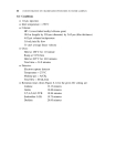
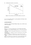
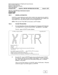
238
DETERMINATION OF INORGANIC AND ORGANIC SOLIDS IN WATER SAMPLES
Obtaining Your Total Solids Measurement
4. Add 100 mL of your sample to your crucible and evaporate it in the 98 C
oven overnight.
5. Place your crucible in the 104 C oven the next day and bake it for
1 hour.
6. Place the crucible in a desiccator until cool and obtain a constant
weight.
7. Repeat steps 5 and 6 until you obtain a constant weight (within 0.5 mg of
each other). This will be the total solids measurement (box 1 in Figure 20-1):
TSðmg=LÞ
ðaverage final weight in g average initial crucible weight empty in gÞð1000 mg=gÞ
¼
sample volume in L
Obtaining Your Fixed and Volatile Solids Measurements
8. Place the crucible from step 7 in the muffle furnace at 550 C for 30 minutes.
9. Obtain a constant weight for the crucibles by allowing the crucibles to cool
almost completely on a benchtop and then to cool completely in a
desiccator, weighing to a constant weight, and repeating the heating and
cooling process until you have two weights within 0.6 mg or less of each
other. This measurement will yield your fixed solids and volatile solids
measurements (box 2 in Figure 20-1).
FSðmg=LÞ
ðaverage final weight from step 9 in g average initial crucible weight empty in gÞð1000 mg=gÞ
¼
sample volume in L
VSðmg=LÞ
ðaverage initial crucible weight from step 7 in g average final weight from step 9 in gÞð1000 mg=gÞ
¼
sample volume in L
Group II: Total Suspended Solids (TSS) and Suspended Volatile
Solids (SVS) (Boxes 3 and 4 in Figure 20-1)
Overview. In this procedure you will be taking 100 mL of your sample and
performing the most commonly used solids measurement, the total suspended
solids. This requires you to filter a known volume of sample through a preheated
and pretared glass-fiber filter. The difference in weights (final–initial) divided by
the volume of sample will yield the TSS. The TSS measurement accounts for
all solids that do not pass through the filter (typically, 0.45 to 1 mm in size),
weighed after drying at 104 C. When the filter is further dried to 550 C, you
will oxidize any organic matter present in the solids and can obtain a suspended
volatile solids measurement. Thus, you will be completing boxes 3 and 4 in
Figure 20-1.
PROCEDURE
239
Step-by-Step Instructions
Preparing the Filters
1. Rinse three filters with 20 to 30 mL of deionized water to remove any
solids that may remain from the manufacturing process. Place each filter
in a separate, labeled aluminum weight pan, dry them in a 550 C
muffle furnace for 30 minutes, place them (filter and pan) in a desiccator, and obtain a constant weight by repeating the oven and desiccation
steps.
Obtaining the TSS Measurement
2. Filter 100 mL of sample through each filter.
3. Place each filter paper in the aluminum weight pan in the 104 C oven for
1 hour. Cool the filter and pan in a desiccator and obtain a constant weight
by repeating the drying and desiccation steps. This procedure will yield the
TSS measurement (box 3 in Figure 20-1):
TSSðmg=LÞ
ðaverage weight from step 3 in g average inital weight from step 1 in gÞð1000 mg=LÞ
¼
sample volume in L
Obtaining the SVS Measurement
4. Place the filters (in the pan) from step 3 in a muffle furnace at 550 C for 30
minutes. (Depending on the type of muffle furnace you have, you may need
to cover the samples with another weigh pan to avoid contamination of your
sample by ceramic dust.) Remove the filters, place them in a desiccator, and
obtain a constant weight by repeating the muffling and desiccation steps.
This will yield the SVS measurement (box 4 in Figure 20-1):
SVSðmg=LÞ
¼
ðaverage weight from step 3 in g average weight from step 4 in gÞð1000 mg=LÞ
sample volume in L
Group III: Total Dissolved Solids (TDS) and Dissolved Volatile
Solids (DVS) (Boxes 5 and 6 in Figure 20-1)
Overview. In this procedure you will perform the second-most-common solids
measurement, the total dissolved solids. This is determined by first performing a
TSS measurement, but you do not have to weigh the filter as Group II had to do.
240
DETERMINATION OF INORGANIC AND ORGANIC SOLIDS IN WATER SAMPLES
You are only concerned with removing the filterable solids from your sample and
collecting the filtrate. In case you do not have a crucible that will hold 100 mL,
you can add 50 mL of the filtrate, dry the sample to dryness, and add another
50-mL aliquot. You will first evaporate the sample filtrate to dryness in a 98 C
oven, to avoid boiling or splattering, which could result in a loss of sample. Next,
you will take the dried filtrate and crucible and dry it at 104 C to obtain the
mass of dissolved solids in your sample. Finally, you will bake the sample at
550 C to oxidize the organic matter and obtain a dissolved volatile solids
measurement.
Step-by-Step Instructions
Preparing the Crucibles
1. Wash and clean at least three crucibles. You only need three crucibles, but
some of these may crack in the preparation steps, so it is wise to have more
prepared than are needed. Some residue may remain from previous experiments.
2. Label each crucible if they are not already labeled. A good way to label
crucibles is to paint a number on the bottom using an iron oxide paste. When
you bake the crucible, the iron will bind permanently to the crucible. Allow
the crucibles to dry completely prior to placing them in the muffle furnace.
After air drying, dry the crucibles in the muffle furnace at 550 C for
30 minutes (the 30 minutes refers to the total time at 550 C).
3. Obtain a constant weight of the crucibles by drying at 550 C, allow the
crucible to cool almost completely on a benchtop and then to cool
completely in a desiccator, weigh to a constant weight, and repeat the
heating and desiccation processes until you have two weights within 0.6 mg
or less of each other.
Obtaining the Total Dissolved Solids Measurement
4. Add 100 mL of your filtered sample to your crucible and evaporate it in the
98 C oven overnight.
5. Place your crucible in the 104 C oven the next day and bake it for
1 hour.
6. Place the crucible in a desiccator until cool and obtain a constant
weight.
7. Repeat steps 5 and 6 until you obtain a constant weight (within 0.5 mg of
each other). This will be the total dissolved solids measurement (box 5 in
Figure 20-1):
TDSðmg=LÞ
ðaverage crucible weight from step 7 in g average crucible weight empty in gÞð1000 mg=gÞ
¼
sample volume in L
PROCEDURE
241
Obtaining the Volatile Dissolved Solids Measurements
8. Place the crucible from step 7 in the muffle furnace at 550 C for 30 minutes.
9. Obtain a constant weight of the crucibles by allowing the crucible to cool
almost completely on a benchtop and then to cool completely in a
desiccator, weighing to a constant weight, and repeating the heating and
desiccation processes until you have two weights within 0.6 mg or less of
each other. This measurement will yield your total volatile solids measurements (box 6 in Figure 20-1):
DVSðmg=LÞ
ðaverage final crucible weight from step 7 in g average crucible weight from step 9 in gÞð1000 mg=gÞ
¼
sample volume in L
Additional Procedure
If you have a conductivity meter, you will also be measuring the conductivity of
the entire water sample. The conductivity of a sample is a measure of the
dissolved salt concentration (TDS), but the conductivity depends on type of ions
(monodivalent, divalent, etc.), their concentration, and the temperature. In
general,
TDS ¼ conductivity ðmmhos=cmÞ K
where K is a constant ranging from 0.55 to 0.90, depending on the ions in solution
and the temperature. Calibrate the conductivity meter using the 0.00100 M KCl
solution. This solution should have a conductivity of 146.9 mS/cm, and the
0.00500 KCl solution should have a conductivity of 717.5 mS/cm at 25 C.
Make sure that the meter’s automatic temperature compensation function is
turned on.
1. Measure and record the conductivity of the sample. If the conductivity of the
sample is nearer to 700 mS/cm than to 150 mS/cm, recalibrate the meter
with the higher concentration standard.
2. Change the meter from conductivity to TDS mode and measure the TDS of
your sample. Note that this meter uses a K value of 0.5 to estimate TDS
from conductivity. This assumes that the only ions present in solution are Na
and Cl. The TDS value reported by the meter has units of mg/L.
3. Compare your conductivity value to your measured TDS value.
If you have a turbidity meter, you will also be measuring the turbidity of your
original sample. Turbidity is a measure of the light scattered by suspended
particles, especially the clay particles in the sample. Turbidity is measured by a
photoelectric detector aligned at a 90 angle from the light source. Turbidity,
measured in nephelometer turbidity units (NTUs), is a function of particle size,
shape, and concentration. Turbidity is only a quick field approximation of total
242
DETERMINATION OF INORGANIC AND ORGANIC SOLIDS IN WATER SAMPLES
suspended solids. Consult the user’s manual and measure the turbidity of your
sample. Compare this to your TSS measurement.
Hints for Success
Always, always mix your sample completely before removing any solution
or suspension. The clay particles will settle and bias your results if you do
not mix the sample completely every time you remove an aliquot.
Normally in this laboratory manual you will not be given data collection
sheets, but due to the complicated nature of this experiment, a data sheet is
supplied on your CD. Each group should complete the data sheet for the
experiments that you conduct and share the results with your instructor and
the other groups.
Perform all measurements in triplicate.
Carefully clean all containers and prewash all filters with deionized water
prior to use. As the procedure section notes, heat all of these to the maximum
temperature that you will use before obtaining weights. Also as noted in the
procedure, you must obtain a constant weight (generally within 0.5 mg of
each other) before you end each experiment. (Fingerprints and dust weigh
enough to affect your results significantly.)
Your balances have been calibrated, but for best results you should use the
same balance for every measurement. Even if the calibration on a balance is
slightly off, the change in weight will probably be accurate.
ASSIGNMENT
243
ASSIGNMENT
Complete the data sheet included with this laboratory procedure. In addition to the
TS, FS, VS, SVS, and DVS calculations, you should answer the questions located
on the bottom of the data collection sheet on the enclosed CD. Based on your
results, also summarize the mass of particulate matter, inorganic salts, and organic
matter in your 1.00-L sample.
DATA COLLECTION SHEET
21
DETERMINATION OF ALKALINITY
OF NATURAL WATERS
Purpose: To determine the alkalinity of a natural water sample by titration
BACKGROUND
Alkalinity is a chemical measurement of a water’s ability to neutralize acids.
Alkalinity is also a measure of a water’s buffering capacity or its ability to resist
changes in pH upon the addition of acids or bases. The alkalinity of natural waters
is due primarily to the presence of weak acid salts, although strong bases may also
contribute in industrial waters (i.e., OH). Bicarbonates represent the major form
of alkalinity in natural waters and are derived from the partitioning of CO2 from the
atmosphere and the weathering of carbonate minerals in rocks and soil. Other salts
of weak acids, such as borate, silicates, ammonia, phosphates, and organic bases
from natural organic matter, may be present in small amounts. Alkalinity, by
convention, is reported as mg/L CaCO3, since most alkalinity is derived from the
weathering of carbonate minerals rather than from CO2 partitioning with the atmosphere. Alkalinity for natural water (in molar units) is typically defined as the sum
of the carbonate, bicarbonate, hydroxide, and hydronium concentrations such that
þ
½alkalinity ¼ 2½CO2
3 þ ½HCO3 þ ½OH ½H3 O ð21-1Þ
Alkalinity values can range from zero from acid rain–affected areas, to less
than 20 mg/L for waters in contact with non-carbonate-bearing soils, to 2000 to
Environmental Laboratory Exercises for Instrumental Analysis and Environmental Chemistry
By Frank M. Dunnivant
ISBN 0-471-48856-9 Copyright # 2004 John Wiley & Sons, Inc.
245
246
DETERMINATION OF ALKALINITY OF NATURAL WATERS
4000 mg/L for waters from the anaerobic digestors of domestic wastewater
treatment plants (Pohland and Bloodgood, 1963).
Neither alkalinity nor acidity, the converse of alkalinity, has known adverse
health effects, although highly acidic or alkaline waters are frequently considered
unpalatable. However, alkalinity can be affected by or affect other parameters.
Below are some of the most important effects of alkalinity.
1. The alkalinity of a body of water determines how sensitive that water body
is to acidic inputs such as acid rain. A water with high alkalinity better
resists changes in pH upon the addition of acid (from acid rain or from an
industrial input). We discuss this further when we discuss the relevant
equilibrium reactions.
2. Turbidity is frequently removed from drinking water by the addition of
alum, Al2(SO4)3, to the incoming water followed by coagulation, flocculation, and settling in a clarifier. This process releases Hþ into the water
through the reaction
Al3þ þ 3H2 O ! AlðOHÞ3 þ 3Hþ
ð21-2Þ
For effective and complete coagulation to occur, alkalinity must be present
in excess of that reacted with the Hþ releases. Usually, additional alkalinity,
in the form of Ca(HCO3)2, Ca(OH)2, or Na2CO3 (soda ash), is added to
ensure optimum treatment conditions.
3. Hard waters are frequently softened by precipitation methods using CaO
(lime), Na2CO3 (soda ash), or NaOH. The alkalinity of the water must be
known in order to calculate the lime, soda ash, or sodium hydroxide
requirements for precipitation.
4. Maintaining alkalinity is important to corrosion control in piping systems.
Corrosion is of little concern in modern domestic systems, but many main
water distribution lines and industrial pipes are made of iron. Low-pH
waters contain little to no alkalinity and lead to corrosion in metal pipe
systems, which are costly to replacement.
2
5. Bicarbonate ðHCO
3 Þ and carbonate ðCO3 Þ can complex other elements and
compounds, altering their toxicity, transport, and fate in the environment. In
general, the most toxic form of a metal is its uncomplexed hydrated metal
ion. Complexation of this free ion by carbonate species can reduce toxicity.
THEORY
As mentioned previously, alkalinity in natural water is due primarily to carbonate
species. The following set of chemical equilibria is established:
CO2 þ H2 O , H2 CO
3
H2 CO3 ,
HCO
3 ,
þ
HCO
3 þH
þ
CO2
3 þH
ð21-3Þ
ð21-4Þ
ð21-5Þ
247
THEORY
where H2CO
3 represents the total concentration of dissolved CO2 and H2CO3.
Reaction (21-3) represents the equilibrium of CO2 in the atmosphere with
dissolved CO2 in the water. The equilibrium constant, using Henry’s law, for
this reaction is
KCO2 ¼
½H2 CO3 ¼ 4:48 105 M=mmHg
PCO2
ð21-6Þ
The equilibrium expressions for reactions (21-4) and (21-5) are
K1 ¼
½Hþ ½HCO
3
¼ 106:37
½H2 CO3 ð21-7Þ
K2 ¼
½Hþ ½CO2
3 ¼ 1010:32
½HCO3 ð21-8Þ
As you can see from equations (21-6) to (21-8), the important species contributing
to alkalinity are CO2
3 , HCO3 , and H2CO3, and each of these reactions is tied
strongly to pH. To illustrate the importance of these relations, we will calculate
the pH of natural rainwater falling through Earth’s atmosphere that currently
contains 380 ppm CO2.
First, we convert the concentration of CO2 in the air to mol /L (step 1), and then
calculate its partial pressure for use in equation (21-6) (step 2). This enables us to
calculate the molarity of carbon dioxide in water [the [H2CO3] term in equation
(21-6)] (step 3), and then the molarity of H2CO3 in the water (step 4). Finally, we
calculate the pH of the water, based on the equilibrium established between the
different species of dissolved carbonate (step 4).
Step 1:
density of air ¼ 0:001185 g=mLð1000 mL=LÞ ¼ 1:185 g=L
CO2 ðairÞ ¼ 380 mg CO2 =kg air
¼ 380 mg CO2 =kg airð1 kg air=1000 g airÞð1:185 g=LÞ
¼ 0:450 mg CO2 =L
0:450 mg=Lð1 g=1000 mgÞð1 mol CO2 =44 g CO2 Þ
¼ 1:02 105 M CO2 in air
Step 2: Using PV ¼ nRT (note that n=V ¼ M) gives us
PCO2 ¼ MRT ¼ ð1:02 105 mol=LÞð0:08206 L M=mol KÞð298:14 KÞ
¼ 2:50 104 atm
248
DETERMINATION OF ALKALINITY OF NATURAL WATERS
Step 3: Using KCO2 ¼ ½CO2 H2 O =PCO2 ¼ 4:48 105 M=mmHg yields
PCO2 ðmmHgÞ ¼ 2:50 104 atm ð760 mmHg=atmÞ ¼ 0:19 mmHg
KCO2 ¼ 4:48 105 M=mmHg ¼ MCO2 =PCO2
MCO2 in water ¼ 4:48 105 M=mmHg ð0:19 mmHgÞ
¼ 8:52 106 M CO2
Step 4: From step 3, CO2 ðaqÞ ¼ 8:52 106 M;
CO2 ðgÞ þ H2 O , H2 CO3
K¼
K ¼ 1:88
½H2 CO3 CO2 ðaqÞ
½H2 CO3 ¼ 1:88ð8:52 106 MÞ
¼ 1:6 105 M H2 CO3
Step 5: Now, solving for pH using the equilibrium expression for H2CO3, we
obtain
H2 CO3 þ H2 O , H3 Oþ þ HCO
3
Ka ¼ 4:2 107 ¼
4:2 107 ¼
Ka ¼ 4:2 107
½H3 Oþ ½HCO
3
½H2 CO3 x2
1:6 105 x
and using the quadratic equation to solve for x yields
x ¼ ½H3 Oþ ¼ 2:59 106
pH ¼ 5:59
pH of natural rainwater
We can also solve for the remaining chemical species using equilibrium
equations.
6
M HCO
½HCO
3 ¼ x also; so½HCO3 ¼ 2:59 10
3
½H2 CO3 ¼ 1:6 105 ðtotal carbonic concentrationÞ
2:59 106 ¼ 1:3 105 M
2
þ
HCO
3 þ H2 O , CO3 þ H3 O
11
½CO2
M
3 ¼ 4:8 10
Ka ¼ 4:8 1011
REFERENCES
249
Summarizing yields
½H3 Oþ ¼ 2:59 106 M
5
½H2 CO3 ¼ 1:6 10
pH ¼ 5:59
M
6
½HCO
M
3 ¼ 2:59 10
11
M
½CO2
3 ¼ 4:88 10
Thus, a pH value of less than 5.6 for a rain or snow sample is due to mineral
acids from atmospheric pollution or volcanic emissions. Interaction of less acidic
precipitation with soil minerals usually adds alkalinity and raises the pH value,
which counteracts the use of carbon dioxide by algae during daylight hours. If the
consumption rate of CO2 is greater than its replacement rate from the atmosphere,
as can occur when acid precipitation is input, the dissolved CO2 concentration in
the surface water and groundwater will fall and result in a shift to the left for the
corresponding equilibrium reactions:
CO2 ðaqÞ þ H2 O , H2 CO3
þ
H2 CO3 þ H2 O , HCO
3 þ H3 O
This will also result in an increase in the pH of the water. As the pH continues to
increase, the alkalinity changes chemical species to replace the CO2 consumed by
the algae. Note the equilibrium shifts toward increased CO2 concentrations, which
is illustrated in the following reactions
2
2HCO
3 , CO3 þ H2 O þ CO2
CO2
3 þ H2 O , 2OH þ CO2
It should be noted that even though we are creating hydroxide alkalinity, the total
alkalinity has not changed, merely shifted in chemical form. We define hydroxide
alkalinity later as alkalinity in excess of a pH value of 10.7. Algae can continue to
consume CO2 until the pH of the water has risen to between 10 and 11, when a
growth inhibitory pH is reached and algae consumption of CO2 is halted. This can
result in a diurnal shift in the pH of the photic zone of a water body. In waters
containing significant calcium concentrations, the set of reactions above can result
in the precipitation of CaCO3 on leaves and twigs in water, and in the long term,
can lead to the formation of marl deposits in sediments. Thus, even algae can
produce the industrial-sounding ‘‘hydroxide alkalinity.’’
REFERENCES
American Water Works Association, Standard Methods for the Examination of Water and Wastewater
18th ed., AWWA, Denver, CO, 1992.
250
DETERMINATION OF ALKALINITY OF NATURAL WATERS
Harris, D. C., Quantitative Chemical Analysis, 5th ed., W. H. Freeman, New York, 1998.
Keith, L. H., Compilation of EPA’s Sampling and Analysis Methods, Lewis Publishers, Chelsea, MI,
1992.
Pohland, F. G. and D. E. Bloodgood, J. Water Pollut. Control Fed., 35, 11 (1963).
Snoeyink, V. L. and D. Jenkins, Water Chemistry, Wiley, New York, 1980.
Sawyer, C. N. and P. L. McCarty, Chemistry for Environmental Engineering, 3rd ed., McGraw-Hill,
New York, 1978.
Stumm W. and J. J. Morgan, Aquatic Chemistry, 3rd ed., Wiley, New York, 1995.
IN THE LABORATORY
251
IN THE LABORATORY
To determine the alkalinity, a known volume of water sample is titrated with a
standard solution of strong acid to a pH value of approximately 4 or 5. Titrations
can be used to distinguish between three types of alkalinity: hydroxide, carbonate,
and bicarbonate alkalinity. Carbonate alkalinity is determined by titration of the
water sample to the phenolphthalein or metacresol purple indicator endpoint,
approximately pH 8.3. Total alkalinity is determined by titration of the water
sample to the endpoint of the methyl orange, bromocresol green, or bromocresol
green–methyl red indicators, approximately pH 4.5. The difference between the
two is the bicarbonate alkalinity. Hydroxide (OH) alkalinity is present if the
carbonate, or phenolphthalein, alkalinity is more than half of the total alkalinity
[American Water Works Association (AWWA), 1992]. Thus, the hydroxide
alkalinity can be calculated as two times the phenolphthalein alkalinity minus
the total alkalinity.
Note that only approximate pH values can be given for the final endpoint,
which occurs near a pH value of 4.5. This is because the exact endpoint at the end
of the titration, the equivalence point, is dependent on the total concentration of
carbonate species in solution, while the indicator color change is referred to as the
endpoint. The endpoint is subject to the pH value only where the indicator
changes color and is not influenced by the total alkalinity in solution, whereas the
equivalence point is inversely related to alkalinity, with higher total alkalinity
corresponding to equivalence at a lower pH value. This can be explained by
looking at a pC–pH diagram of the carbonate system. A pC–pH exercise is
included in this manual (Chapter 23), and a pC–pH program is included on the
accompanying CD-ROM. Figure 21-1 is for a 0.0010 M total carbonate system.
The exact equivalence point for the alkalinity titration occurs when the Hþ
concentration equals the HCO
3 concentration. For the 0.001 M carbonate solution
(Figure 21-1), this corresponds to the location of the arrow at pH 4.67. As the
carbonate concentration increases to 0.10 M (Figure 21-2), the carbonate species
lines shift to yield an interception at a pH value of 3.66. This is a significant
difference in equivalence points but is not reflected in the indicator endpoint. As a
result, the equivalence points described below have been suggested. The following
endpoints, corresponding to total alkalinity concentrations, are suggested in AWWA
(1992): pH 5.1 for total alkalinities of about 50 mg/L, pH 4.8 for 150 mg/L, and
pH 4.5 for 500 mg/L.
Two points should be noted about the titration curve (again, refer to the pC–pH
diagrams in Figures 21-1 and 21-2).
1. At pH 10.7, the [HCO
3 ] equals the [OH ]. This is called an equivalence
point and is the endpoint of the caustic alkalinity and total acidity titrations.
At pH 8.3, the [H2CO3] equals the [CO2
3 ]. This is the endpoint for
carbonate alkalinity and CO2 acidity titrations. In the alkalinity titration
virtually all of the CO2
3 has reacted (thus, the term carbonate alkalinity)
and half of the HCO2
3 has reacted at the endpoint.
252
DETERMINATION OF ALKALINITY OF NATURAL WATERS
0
1
2
3
0
1
2
3
4
5
6
pC 7
8
9
10
11
12
13
14
4
5
pH
7
6
8
9
10
11
12
13 14
pC/pH of a Closed System
pH = 4.643
Approximated
Non-Printable
Enter the concentration and pKas:
Concentrations must be between
0.00000001 and 1
Concentration = 0.001
pKa 1 =
6.35
pKa 2 =
10.33
pKa 3 =
12
Molar concentration of species at cursor:
1.00e-14
[H2A]
9.80e-4
[HA– ]
2.03e-5
[A2– ]
4.41e-11
Figure 21-1. pC–pH diagram for a 0.001 M carbonate solution. Refer to and use the pC–pH
simulator, which will give color lines on the plot.
0
0
1
2
3
4
5
6
pC 7
8
9
10
11
12
13
14
1
2
3
4
5
6
pH
7
8
9
10
11
12
13
14
pC/pH of a
Closed System
pH = 3.640
Approximated
Enter the concentration and pKas:
Concentrations must be between
0.00000001 and 1
Concentration =
0.01
pKa 1 =
6.35
pKa 2 =
10.33
pKa 3 =
12
Non-Printable
Molar concentration of species at cursor:
[H2A]
[HA– ]
[A2– ]
1.00e-14 0.0998 1.95e-4 397e-11
Figure 21-2. pC–pH diagram for a 0.10 M carbonate solution. Refer to and use the pC–pH
simulator, which will give color lines on the plot.
IN THE LABORATORY
253
2. At pH 4.5 (dependent on the total alkalinity), the [Hþ] equals the [HCO
3 ].
This is the endpoint for mineral acidity and total alkalinity titrations.
Safety Precautions
As in all laboratory exercises, safety glasses must be worn at all times.
Avoid skin and eye contact with NaOH and HCl solutions. If contact occurs,
rinse your hands and/or flush your eyes for several minutes. Seek immediate
medical advice for eye contact.
Use concentrated HCl in the fume hood and avoid breathing its vapor.
Chemicals and Solutions
Sample Handling. Alkalinity is a function of the dissolved CO2 in solution.
Thus, any chemical or physical manipulation of the sample that will affect the
CO2 concentration should be avoided. This includes filtering, diluting, concentrating, or altering the sample in any way. Nor should the sampling temperature be
exceeded, as this will cause dissolved CO2 to be released. Samples containing oil
and grease should be avoided. Sampling and storage vessels can be plastic or glass
without headspace.
Sodium carbonate solution, 0.025 M. Primary standard grade Na2CO3
must be dried for 3 to 4 hours at 250 C and be allowed to cool in a desiccator.
Weigh 0.25 g to the nearest 0.001 g and quantitatively transfer all of the solid
to a 100-mL volumetric flask. Dilute to the mark with distilled or deionized
water. Calculate the exact molarity of the solution in the 100-mL flask.
Standardized hydrochloric acid (about 0.02 M). Add 8.3 mL of concentrated
(12 M) HCl to a 1000-mL volumetric flask and dilute to the mark with
deionized or distilled water. This solution has a molarity of approximately
0.10 M. Transfer 200 mL of this solution to another 1000-mL volumetric
flask to prepare the 0.020 M solution. Standardize the dilute HCl solution
(about 0.020 M) against the Na2CO3 primary standard solution. This is done
by pipetting 10.00 mL of the 0.025 M Na2CO3 solution into a 250-mL
Erlenmeyer flask and diluting to about 50 mL with distilled or deionized
water. Add 3 to 5 drops of the bromocresol green indicator (more if needed)
to the Erlenmeyer flask and titrate with 0.02 M HCl solution. Bromocresol
green changes from blue to yellow as it is acidified. The indicator endpoint is
intermediate between blue and yellow, and appears as a distinct green color.
Determine the molarity of the HCl solution. Remember to wash down any
droplets of solution from the walls of the flask.
Bromocresol green indicator solution, about 0.10%, pH 4.5 indicator.
Dissolve 0.100 g of the sodium salt into 100 mL of distilled or deionized
water. Colors: yellow in acidic solution, blue in basic solution.
254
DETERMINATION OF ALKALINITY OF NATURAL WATERS
Phenolphthalein solution, alcoholic, pH 8.3 indicator. Colors: colorless in
acidic solution, red in basic solution.
Metacresol purple indicator solution, pH 8.3 indicator. Dissolve 100 mg of
metacresol purple in 100 mL of water. Colors: yellow in acidic solution,
purple in basic solution.
Mixed bromocresol green–methyl red indicator solution. You may use either
the water- or alcohol-based indicator solution. Water solution: dissolve 100
mg of bromocresol green sodium salt and 20 mg of methyl red sodium salt in
100 mL of distilled or deionized water. Ethyl or isopropyl alcohol solution:
dissolve 100 mg of bromocresol green and 20 mg of methyl red in 100 mL of
95% alcohol.
Glassware
Standard laboratory glassware: 50-mL buret, 250-mL Erlenmeyer flasks,
50-mL beakers, Pasteur pipets
PROCEDURE
255
PROCEDURE
Limits of the Method. Typically, 20 mg of CaCO3/L. Lower detection limits can
be achieved by using a 10-mL microburet (Keith, 1992)
1. First, an adequate sample volume for titration must be determined. This is
accomplished by performing a test titration. Select a volume of your sample,
such as 100 mL, and titrate it to estimate the total alkalinity of your sample.
For best accuracy, you should use at least 10 mL but not more than 50 mL
from a 50-mL buret. Adjust your sample size to meet these criteria.
2. Titrate your sample with standardized 0.02 M HCl solution. Add phenolphthalein or metacresol purple indicator solution and note the color
change around a pH value of 8.3. Alternatively, a pH meter can be used to
determine the inflection point. This measurement will be a combination of
the hydroxide and carbonate alkalinity.
3. Continue the titration to the 4.5 endpoint by adding bromocresol green or
the mixed bromocresol green–methyl red indicator solution. Better results
will be obtained by titrating a new sample to the 4.5 endpoint. This will
avoid potential color interferences between the 8.3 and 4.5 pH indicators.
Note the color change near a pH value of 4.5. Alternatively, a pH meter can
be used to determine the inflection point.
4. Repeat steps 2 and 3 at least three times (excluding the trial titration to
determine your sample volume).
5. Calculate the hydroxide, carbonate, bicarbonate, and total alkalinities for
your samples. Report your values in mg CaCO3/L. Show all calculations in
your notebook.
Waste Disposal
After neutralization, all solutions can be disposed of down the drain with water.
256
DETERMINATION OF ALKALINITY OF NATURAL WATERS
ADVANCED STUDY ASSIGNMENT
1. In your own words, define alkalinity and explain why it is important in
environmental chemistry.
2. What are the primary chemical species responsible for alkalinity in natural
waters?
3. Alkalinity can be expressed in three forms: hydroxide alkalinity, carbonate
alkalinity, and total alkalinity. Each of these is determined by titration, but at
different pH values. What is the approximate endpoint pH for the carbonate
alkalinity titration? What is the approximate endpoint pH for the total
alkalinity titration?
4. Why can we give only approximate pH endpoints for each type of alkalinity?
5. To prepare yourself for the laboratory exercise, briefly outline a procedure
for titrating a water sample for alkalinity. (List the major steps.)
6. If you titrate 200 mL of a sample with 0.0200 M HCl and the titration takes
25.75 mL of acid to reach the bromocresol green endpoint, what is the total
alkalinity of the sample?
7. The atmospheric concentration of CO2 is predicted to increase up to 750 ppm
by the year 2100. What will be the pH of rainwater if it is in equilibrium
with an atmosphere containing 500 ppm CO2?
22
DETERMINATION OF HARDNESS
IN A WATER SAMPLE
Purpose: To learn the EDTA titration method for determining the hardness of a
water sample
BACKGROUND
In the past, water hardness was defined as a measure of the capacity of water to
precipitate soap. However, current laboratory practices define total hardness as the
sum of divalent ion concentrations, especially those of calcium and magnesium,
expressed in terms of mg CaCO3/L. There are no known adverse health effects of
hard or soft water, but the presence of hard waters results in two economic
considerations: (1) hard waters require considerably larger amounts of soap to
foam and clean materials, and (2) hard waters readily precipitate carbonates
(known as scale) in piping systems at high temperatures. Calcium and magnesium
carbonates are two of the few common salts whose solubility decreases with
increasing temperature. This is due to the removal of dissolved CO2 as temperature increases. The advent of synthetic detergents has significantly reduced the
problems associated with hard water and the ‘‘lack of foaming.’’ However, scale
formation continues to be a problem.
The source of a water sample usually determines its hardness. For example,
surface waters usually contain less hardness than do groundwaters. The hardness
of water reflects the geology of its source. A color-coded summary of water
hardness in the United States can be found at http://www.usgs.org, and if
Environmental Laboratory Exercises for Instrumental Analysis and Environmental Chemistry
By Frank M. Dunnivant
ISBN 0-471-48856-9 Copyright # 2004 John Wiley & Sons, Inc.
257
258
DETERMINATION OF HARDNESS IN A WATER SAMPLE
TABLE 22-1. Correlation of Water Hardness Values
with Degrees of Hardness
mg CaCO3/L Hardness
0–75
75–150
150–300
>300
Degree of Hardness
Soft
Moderately hard
Hard
Very hard
you view this map you will see that hardness values can range from less than
50 mg/L to over 250 mg/L. Therefore, depending on your water’s source, some
modifications to the procedure described below may be necessary. Carbonates in
surface soils and sediments increase the hardness of surface waters, and subsurface limestone formations also increase the hardness of groundwaters. As
indicated in Table 22-1, hardness values can range from a few to hundreds of
milligrams of CaCO3 per liter.
The divalent metal cations responsible for hardness can react with soap to form
precipitates, or when the appropriate anions are present, to form scale in hot-water
pipes. The major hardness-causing cations are calcium and magnesium, although
strontium, ferrous iron, and manganese can also contribute. It is common to
compare the alkalinity values of a water sample to the hardness values, with both
expressed in mg CaCO3/L. When the hardness value is greater than the total
alkalinity, the amount of hardness that is equal to the alkalinity is referred to as the
carbonate hardness. The amount in excess is referred to as the noncarbonate
hardness. When the hardness is equal to or less than the total alkalinity, all
hardness is carbonate hardness and no noncarbonate hardness is present. Common
cations and their associated anions are shown in Table 22-2.
THEORY
The method described below relies on the competitive complexation of divalent
metal ions by ethylenediaminetetraacetic acid (EDTA) or an indicator. The
TABLE 22-2. Common Cation–Anion Associations
Affecting Hardness and Alkalinity
Cations Yielding Hardness
2þ
Ca
Mg2þ
Sr2þ
Fe2þ
Mn2þ
Associated Anions
HCO
3
SO2
4
Cl
NO
3
SiO2
3
REFERENCES
NaOOC CH2
HOOC CH2
259
CH2 COONa
H H
N C C N
H H
CH2 COOH
Figure 22-1. Chemical structure for the disodium salt of EDTA.
chemical structure for the disodium salt of EDTA is shown in Figure 22-1. Note
the lone pairs of electrons on the two nitrogens. These, combined with the
dissociated carboxyl groups, create a 1 : 1 hexadentate complex with each divalent
ion in solution. However, the complexation constant is a function of pH (Harris,
1999). Virtually all common divalent ions will be complexed at pH values greater
than 10, the pH used in this titration experiment and in most hardness tests. Thus,
the value reported for hardness includes all divalent ions in a water sample.
Three indicators are commonly used in EDTA titration, Eriochrome Black T
(Erio T), Calcon, and Calmagite. The use of Eriochrome Black T requires that a
small amount of Mg2þ ion be present at the beginning of the titration. Calmagite
is used in this experiment because its endpoint is sharper than that of Eriochrome
Black T.
REFERENCES
American Water Works Association, Standard Methods for the Examination of Water and Wastewater,
18th ed., AWWA, Denver, Co, 1992.
Harris, D. C., Quantitative Chemical Analysis, 5th ed., W.H. Freeman and Company, New York,
1998.
Keith, L. H., Compilation of EPA’s Sampling and Analysis Methods, Lewis Publishers, Chelsea, MI,
1992.
Sawyer, C. N. and P. L. McCarty, Chemistry for Environmental Engineering, 3rd ed., McGraw-Hill,
New York, 1978.
Snoeyink, V. L. and D. Jenkins, Water Chemistry, Wiley, New York, 1980.
260
DETERMINATION OF HARDNESS IN A WATER SAMPLE
IN THE LABORATORY
Two methods are available for determining the hardness of a water sample. The
method described and used here is based on a titration method using a chelating
agent. The basis for this technique is that at specific pH values, EDTA binds with
divalent cations to form a strong complex. Thus, by titrating a sample of known
volume with a standardized (known) solution of EDTA, you can measure the
amount of divalent metals in solution. The endpoint of the titration is observed
using a colorimetric indicator, in our case Calmagite. When a small amount of
indicator is added to a solution containing hardness (at pH 10.0), it combines with
a few of the hardness ions and forms a weak wine red complex. During the
titration, EDTA complexes more and more of the hardness ions until it has
complexed all of the free ions and ‘‘outcompetes’’ the weaker indicator complex
for hardness ions. At this point, the indicator returns to its uncomplexed color
(blue for Calmagite), indicating the endpoint of the titration, where only EDTAcomplexed hardness ions are present.
Safety Precautions
As in all laboratory exercises, safety glasses must be worn at all times.
Avoid skin and eye contact with pH 10 buffer. In case of skin contact, rinse
the area for several minutes. For eye contact, flush eyes with water and seek
immediate medical advice.
Chemicals and Solutions
Sample Handling. Plastic or glass sample containers can be used. A minimum of
100 mL is needed, but for replicate analysis of low-hardness water, 1 L of sample
is suggested. If you are titrating the sample on the day of collection, no
preservation is needed. If longer holding times are anticipated, the sample can
be preserved by adding nitric or sulfuric acid to a pH value of less than 2.0. Note
that this acidic pH level must be adjusted to above a pH value of 10 before the
titration.
pH 10 buffer. In a 250-mL volumetric flask, add 140 mL of a 28% by weight
NH3 solution to 17.5 g of NH4Cl and dilute to the mark.
Calmagite [1-(1-hydroxy-4-methyl-2-phenylazo)-2-naphthol-4-sulfonic acid].
Dissolve 0.10 g of Calmagite in 100 mL of distilled or deionized water. Use
about 1 mL per 50-mL sample to be titrated.
Analytical reagent-grade Na2EDTA (FW 372.25). Dry at 80 C for 1 hour
and cool in a desiccator. Accurately weigh 3.723 g (or a mass accurate to
0.001 g), dissolve in 500 mL of deionized water with heating, cool to room
IN THE LABORATORY
261
temperature, quantitatively transfer to a 1-L volumetric flask, and fill to the
mark. Since EDTA will extract hardness-producing cations out of most glass
containers, store the EDTA solution in a plastic container. This procedure
produces a 0.0100 M solution.
Glassware
Standard laboratory glassware: 50-mL buret, 250-mL Erlenmeyer flasks,
50-mL beakers, Pasteur pipets
262
DETERMINATION OF HARDNESS IN A WATER SAMPLE
PROCEDURE
Limits of the Method. Detection limits depend on the volume of sample titrated.
1. Pipet an aliquot of your sample into a 250-mL Erlenmeyer flask. The initial
titration will only be a trial and you will probably need to adjust your sample
volume to obtain the maximum precision from your pipetting technique (use
more than 10 mL but less than 50 mL). Increase or decrease your sample
size as needed.
2. Add 3 mL of the pH 10 buffer solution and about 1 mL of the Calmagite
indicator. Check to ensure that the pH of your sample is at or above pH 10.
Add additional buffer solution if needed.
3. Titrate with EDTA solution and note the color change as you reach the
endpoint. Continue adding EDTA until you obtain a stable blue color with
no reddish tinge (incandescent light can produce a reddish tinge at and past
the endpoint).
4. Repeat until you have at least three titrations that are in close agreement.
5. Calculate the hardness for each of your samples. Express your results in mg
CaCO3/L. If you made the EDTA solution exactly according to the
procedure, 1.00 mL of EDTA solution is equal to 1.00 mg CaCO3/L.
Confirm this through calculations.
Waste Disposal
After neutralization, all solutions can be disposed of down the drain with rinsing.
ADVANCED STUDY ASSIGNMENT
263
ADVANCED STUDY ASSIGNMENT
1.
2.
3.
4.
5.
6.
In your own words, define hardness.
What are the primary cations typically responsible for hardness?
In what unit of measure is hardness usually expressed?
What is meant by carbonate and noncarbonate hardness?
What is the color change for the Calmagite indicator?
Briefly outline a procedure for titrating a water sample for hardness. (List
the major steps.)
7. If you titrate 50.0 mL of a sample with 0.100 M EDTA and the titration
takes 25.75 mL of EDTA to reach the endpoint, what is the hardness of the
sample in mg CaCO3/L?
DATA COLLECTION SHEET
PART 7
FATE AND TRANSPORT
CALCULATIONS
23
pC–pH DIAGRAMS: EQUILIBRIUM
DIAGRAMS FOR WEAK ACID
AND BASE SYSTEMS
Purpose: To learn to plot and interpret pC–pH diagrams manually
BACKGROUND
The concentration of a weak acid or base in a solution (e.g., H2CO3, HCO
3 , or
2
CO3 ) can be calculated using simple equilibrium expressions at any given pH. In
some cases it is useful to look at the equilibrium distribution of each of the
protonated and nonprotonated species in solution at the same time. A pC–pH
diagram such as those shown in Figures 23-1 and 23-2 is an excellent tool for
viewing these concentrations simultaneously. As the name implies, the concentrations of all chemical species (including the hydronium ion) are expressed
as the negative log of concentration (for the hydronium ion, the pH). To construct
a pC–pH diagram, the total concentration of the acid or base is needed along with
the corresponding equilibrium equations and constants (K).
CLOSED SYSTEMS
All pC–pH diagrams have two lines in common, the line describing the
concentration of hydroxide (OH) as a function of pH and the line describing
Environmental Laboratory Exercises for Instrumental Analysis and Environmental Chemistry
By Frank M. Dunnivant
ISBN 0-471-48856-9 Copyright # 2004 John Wiley & Sons, Inc.
267
268
pC–pH DIAGRAMS: EQUILIBRIUM DIAGRAMS
0
1
2
3
4
0
1
2
3
4
5
6
pC 7
8
9
10
11
12
13
14
5
6
pH
7
8
9
10
11
12
13
14
pC/pH of a Closed System
Enter the concentration and pKas:
Concentrations must be between
0.00000001 and 1
Concentration =
0.01
pKa 1 =
2.15
pKa 2 =
7.2
pKa 3 =
12.35
Non-Printable
Molar concentration of species at cursor:
[H3A]
[H2A– ]
[HA2– ]
[A3– ]
1.00e-14 1.00e-14 1.00e-14 1.00e-14
Figure 23-1. pC–pH diagram for a triprotic system.
pCpH Help
0
0
1
2
3
4
5
6
pC 7
8
9
10
11
12
13
14
1
2
3
4
5
6
pH
7
8
9
10
11
12
13
14
pC/pH of a Open System
Non-Printable
Molar concentration of species at cursor:
Current system type: Enter the concentration of
atmospheric CO2 or H2S:
[H3CO3] [HCO3] [CO32–]
Total
aerobic
Carbon
Concentration =
380 ppm
1.29e-5
6.31
324
330
Figure 23-2. pC–pH diagram for an open carbonate system.
CLOSED SYSTEMS
269
the concentration of hydronium ion (Hþ) as a function of pH. These are based on
the equilibrium relation
H2 O , Hþ þ OH
where
Kw ¼ ½Hþ ½OH ¼ 1 1014
By rearranging and taking the negative log of each side, we obtain
log Kw ¼ log½Hþ log½OH pOH ¼ 14 pH
The slope of the diagonal line representing the change in [OH] and [Hþ] is
pOH
¼ 1
pH
and when pH equals 0, the pOH equals 14. This results in a line from ( pH 0.0,
pC 14.0) to (pH 14.0, pC 0.0). Similarly, a line can be drawn representing the
hydronium ion concentration as a function of pH. By definition
log½Hþ ¼ pH
Therefore,
ðlog½Hþ Þ
¼1
pH
When the pH equals 0, log½Hþ equals 0. This results in a line from (pH 0.0,
pC 0.0) to (pH 14.0, pC 14.0).
The next line (or set of lines) normally drawn on a pC–pH diagram is the one
representing the total concentration of acid or base, CT . When pC–pH diagrams
are drawn by hand, CT is drawn as a straight horizontal line starting at pCT on the
y axis. This line is actually a combination of two or more lines, depending on the
number of protons present in the acid. At the first pKa (the negative log of the Ka ),
two lines intersect, one with a negative whole-number slope and one with a
positive whole-number slope. For diprotic and triprotic systems, as one species
line crosses a second line (or pKa ), the slope of the line shifts from 1 or þ1 to
2 or þ2, respectively. These lines represent the concentration of each chemical
species. Three cases are given below: a triprotic system (the phosphate system), a
diprotic system (the carbonate system), and a monoprotic system (a generic
system).
270
pC–pH DIAGRAMS: EQUILIBRIUM DIAGRAMS
For a triprotic system, the lines for each individual chemical species can be
represented by
H3 A , H2 A þ Hþ
where K1 ¼
½H2 A ½Hþ ½H3 A
H2 A , HA2 þ Hþ
where K2 ¼
½HA2 ½Hþ ½H2 A HA2 , A3 þ Hþ
where K3 ¼
½A3 ½Hþ ½HA2 The total concentration of the acid or base, CT , is a sum of all protonated and
nonprotonated species, such that
CT ¼ H3 A þ H2 A þ HA2 þ A3
When the equilibrium expressions above and the CT equation are combined and
solved for the concentrations of H3A, H2A, HA2, and A3 in terms of CT , [Hþ],
and the equilibrium constants, four equations are obtained:
1
½H3 A ¼ CT
þ
1 þ ðK1 =½H Þ þ ðK1 K2 =½Hþ 2 Þ þ ðK1 K2 K3 =½Hþ 3 Þ
½H2 A ¼ CT
½HA2 ¼ CT
½A3 ¼ CT
1
ð½H =K1 Þ þ 1 þ ðK2 =½Hþ Þ þ ðK2 K3 =½Hþ 2 Þ
þ
1
þ 2
þ
ð½H =K1 K2 Þ þ ð½H =K2 Þ þ 1 þ ðK3 =½Hþ Þ
1
þ 3
þ 2
ð½H =K1 K2 K3 Þ þ ð½H =K2 K3 Þ þ ð½Hþ =K3 Þ þ 1
If a pH-dependent constant aH is defined as
aH ¼
½Hþ 3
½Hþ 2 ½Hþ þ
þ
þ1
K3
K1 K2 K3 K2 K3
the previous equations can be simplified to:
½H3 A ¼
CT ½Hþ 3
K1 K2 K3 aH
CT ½Hþ 2
K2 K3 aH
þ
C
T ½H ½HA2 ¼
K3 aH
CT
½A3 ¼
aH
½H2 A ¼
CLOSED SYSTEMS
271
Several important points about the pC–pH diagram should be noted.
Figure 23-1 was made for a 0.001 M phosphate system. Note the lines representing the hydrogen and hydroxide ion concentrations, which have a slope of þ1 and
1, respectively. The system points, defined as vertical lines at each pKa value,
represent the pH where each chemical species adjacent to these lines is at equal
concentration. Note that this condition is met at each equilibrium constant (Ka ),
or using the negative log scale, at each pKa value. For the phosphate system
these values are 102.1 for K1, 107.2 for K2, and 1012.3 for K3. Note that at pH
values less than pK1 , the system is dominated by the H3PO4 species; at pH values
between pK1 and pK2 , the system is dominated by the H2 PO
4 ion; at pH values
between pK2 and pK3 , the system is dominated by the HPO24 ion; and at pH
values above pK3 , the system is dominated by the PO3
4 ion. Also note that as the
pH increases, each time the line describing the concentration of a species
approaches a pKa value and crosses another pKa (system point), the slope of
the line decreases by a whole-number value.
For a diprotic system, the equilibrium equations for H2A, HA, and A2 are
H2 A , HA þ Hþ
where K1 ¼
½HA ½Hþ ½H2 A
HA , A2 þ Hþ
where K2 ¼
½A2 ½Hþ ½HA When these equations are combined with the mass balance equation,
CT ¼ H2 A þ HA þ A2
and solved for H2A, HA, and A2 in terms of CT , [Hþ], and the equilibrium
constants, three equations are obtained:
½H2 A ¼ CT
½HA ¼ CT
½A2 ¼ CT
1
1 þ ðK1 =½H Þ þ ðK1 K2 =½Hþ 2 Þ
þ
1
ð½H =K1 Þ þ 1 þ ðK2 =½Hþ Þ
þ
1
þ 2
ð½H =K2 K2 Þ þ ð½Hþ =K2 Þ þ 1
If a pH-dependent constant aH is defined as
aH ¼
½Hþ 2 ½Hþ þ
þ1
K2
K1 K2
272
pC–pH DIAGRAMS: EQUILIBRIUM DIAGRAMS
the previous equations for the diprotic system can be simplified to
½H2 A ¼
CT ½Hþ 2
K1 K2 aH
½HA ¼
CT ½Hþ K2 aH
½A2 ¼
CT
aH
For a monoprotic system, the governing equations are considerably simpler,
since only pKa is involved,
½HA ¼
CT ½Hþ ½Hþ þ Ka
and ½A ¼
CT Ka
½Hþ þ Ka
The utility of a pC–pH diagram is that all of the ion concentrations can be
estimated at the same time for any given pH value. This computer simulation in
the pC–pH computer package included with your manual allows the user to select
an acid system, enter the pKa values, and draw the pC–pH diagram. After the
diagram is drawn, the user can point the cursor at a given pH, and the
concentrations of each ion will be given. Additional discussions of pC–pH
diagrams can be found in Langmuir (1997) and Snoeyink and Jenkins (1980).
OPEN SYSTEMS
The pC–pH diagrams for open systems are similar to those described for closed
systems. The primary difference is that in an open system a component of the
system exists as a gas and the system is open to the atmosphere. In other words,
the system can exchange matter and energy with the atmosphere. The most
important environmental example of such a system comprises carbon dioxide
(CO2), carbonic acid (H2CO3), bicarbonate ion (HCO
3 ), and carbonate ion
2
(CO3 ) in lakes, rivers, and oceans.
The reactions occurring in this system are
CO2 þ H2 O $ H2 CO3
þ
H2 CO3 $ HCO
3 þH
2
þ
HCO
3 $ CO3 þ H
H2 O $ Hþ þ OH
OPEN SYSTEMS
273
The equilibrium relationships for this system are
Kw ¼ ½Hþ ½OH ¼ 1014
KCO2 ¼
½H2 CO3 ¼ 101:47
PCO2
K1 ¼
½Hþ ½HCO
3
¼ 106:35
½H2 CO3 K2 ¼
½Hþ ½CO2
3 ¼ 1010:33
½HCO3 where PCO2 is the partial pressure of CO2 in the atmosphere.
Open system pC–pH diagrams contain lines describing the concentration of
hydroxide (OH) and hydronium ion (Hþ) identical to those for closed systems.
However, because open systems can exchange matter with the atmosphere,
the total inorganic carbon concentration is not constant as it is for a closed
system, but varies as a function of pH. Still, the total inorganic carbon
concentration is the sum of all inorganic carbon species, as it was for closed
systems. In this case,
2
CT ¼ ½H2 CO3 þ ½HCO
3 þ ½CO3 2
The concentration of H2CO3, HCO
3 , and CO3 as a function of pH and PCO2 can
be calculated from the equilibrium relationships given previously. The equations
for these lines are
½H2 CO3 ¼ ðKCO2 ÞðPCO2 Þ ¼ ðPCO2 Þð101:47 Þ
log½H2 CO3 ¼ logðPCO2 Þ þ 1:47
½HCO
3¼
ðK1 ÞðPCO2 Þð101:47 Þ ð106:35 ÞðPCO2 Þð101:47 Þ
¼
Hþ
Hþ
log½HCO
3 ¼ logðPCO2 Þ þ 7:82 pH
½CO2
3 ¼
ðK2 Þð106:35 ÞðPCO2 Þð101:47 Þ
ðHþ Þ2
¼
ð1010:33 Þð106:35 ÞðPCO2 Þð101:47 Þ
ðHþ Þ2
log½CO2
3 ¼ logðPCO2 Þ þ 18:15 2pH
As mentioned previously and demonstrated by the equations above, the con2
centrations of H2CO3, HCO
3 , and CO3 vary as a function of both pH and PCO2 .
This means that as PCO2 has varied naturally over the years during ice ages and
2
periods of warming, the concentration of H2CO3, HCO
3 , and CO3 in surface
274
pC–pH DIAGRAMS: EQUILIBRIUM DIAGRAMS
waters has changed. It also means that PCO2 changes caused by global warming
will alter the surface water concentrations of these species.
A pC–pH diagram for the open carbonate system (380 ppm CO2 in the
atmosphere) is shown in Figure 23-2.
REFERENCES
Langmuir, D., Aqueous Environmental Geochemistry, Prentice Hall, Upper Saddle River, NJ, 1997.
Snoeyink, V. L. and D. Jenkins, Water Chemistry, Wiley, New York, 1980.
ASSIGNMENT
275
ASSIGNMENT
Insert the CD-ROM or install the pC–pH module on your computer (the pC–pH
simulator is included with your lab manual). After you have installed pC–pH, if it
does not start automatically, open it. A sample data set will load automatically.
Work through the example problem, referring to the background information
given earlier and the explanation of the example problem (included in the pC–pH
module) as needed.
1. Why is the slope of the [OH] and [Hþ] lines equal to 1.00 and 1.00,
respectively?
2. Why does the slope of each carbon species shift by one whole-number value
when the line crosses a second pKa value?
3. Using graph paper, draw a pC–pH diagram manually for a closed carbonate
system (total carbonate concentration of 0.0500 M). What is the dominant
carbon species at pH 4.0, 8.0, and 11.0? Calculate the exact molar
concentration of each chemical species at pH 8.00.
4. Using graph paper, draw a pC–pH diagram manually for an open carbonate
system (total atmospheric CO2 concentration of 450 ppm). What is the
dominant carbon species at pH 8.00? Calculate the exact molar concentration of each chemical species at pH 9.50.
To Print a Graph from Fate
For a PC
Select the printable version of your plot (lower right portion of the screen).
Place the cursor over the plot at the desired x and y coordinates.
Hold the alt key down and press print screen.
Open your print or photoshop program.
Paste the Fate graph in your program by holding down the control key and
press the letter v.
Save or print the file as usual.
For a Mac
Select the printable version of your plot.
Hold down the shift and open apple key and press the number 4. This will
place a cross-hair symbol on your screen. Position the cross-hair symbol in
the upper right corner of your plot, click the cursor and drag the cross-hair
symbol over the area to be printed or saved, release the cursor when you
have selected the complete image. A file will appear on your desktop as
picture 1.
Open the file with preview or any image processing file and print it as usual.
24
FATE AND TRANSPORT OF POLLUTANTS
IN RIVERS AND STREAMS
Purpose: To learn two basic models for predicting the fate and transport of
pollutants in river systems
BACKGROUND
The close proximity to natural waterways of chemical factories, railways, and
highways frequently leads to unintentional releases of hazardous chemicals into
these systems. Once hazardous chemicals are in the aquatic system, they can have
a number of detrimental effects for considerable distances downstream from their
source. This exercise allows the user to predict the concentration of a pollutant
downstream of an instantaneous release. Examples of instantaneous releases can
be as simple as small discrete releases such as dropping a liter of antifreeze off a
bridge, or they can be more complex, such as a transportation accident that results
in the release of acetone from a tanker car. Continuous (step) releases usually
involve steady input from an industrial process, drainage from nonpoint sources,
or leachate from a landfill. Once released to the system, the model assumes that
the pollutant and stream water are completely mixed (i.e., there is no crosssectional concentration gradient in the stream channel). This is a reasonably good
assumption for most systems. The model used here accounts for longitudinal
dispersion (spreading in the direction of stream flow), advection (transport in the
direction of stream flow at the flow rate of the water), and a first-order removal
term (biodegradation or radioactive decay).
Environmental Laboratory Exercises for Instrumental Analysis and Environmental Chemistry
By Frank M. Dunnivant
ISBN 0-471-48856-9 Copyright # 2004 John Wiley & Sons, Inc.
277
278
FATE AND TRANSPORT OF POLLUTANTS IN RIVERS AND STREAMS
CONCEPTUAL DEVELOPMENT OF GOVERNING FATE
AND TRANSPORT EQUATION
Instantaneous Pollutant Input
Before we show the mathematical development of the governing equation, we
present a conceptual approach that shows how each part of the equation relates to
a physical model of a polluted river (illustrated in Figure 24-1). The governing
equation for the instantaneous model and a typical concentration–time profile for
this equation are shown in the upper right-hand corner of the figure. The river is
shown flowing from the upper left-hand corner to the lower right-hand corner. The
instantaneous source (W in mass units) is shown upstream in the river as an
irregular by shaped object. This represents a one-time sporadic input of pollutant,
such as a barrel of waste falling in the river or a shipping accident. Upon entry to
the river, the pollutant is mixed rapidly and evenly across the cross section of the
stream. Next, the velocity gradients (v) and flow rate (Q) are shown. As a plume of
pollution is transported down a stream, additional mixing occurs and the length of
the pollutant plume increases. We account for this mixing and dilution of the
pollutant concentration with E, the longitudinal dispersion coefficient (m2/s). This
is easy but costly to measure in a stream, but we can estimate it accurately by
knowing the slope of the stream channel (the decrease in elevation with distance
from the pollutant input point). Next, we are concerned with any first-order
removal of pollutant from the stream and include microbial and chemical
degradations, volatilization, and sorption to river sediments. This accounts for
all of the major processes in the real world and all of the terms shown in the
governing equation. A typical concentration–distance profile for an instantaneous
input is shown in the upper right-hand corner of Figure 24-1, below the instantaneous input model equation.
Instantaneous Input Model
Step
Input
W
C(x) =
Instant.
Input
Q 1+
exp
4kE
4kE
vx
1± 1+
2E
v2
v2
Conc
Q
v
E
E
x, distance
First-Order
Degradation
k
Conc
E
x, distance
Step Input Model
W
C(x) =
Q 1+
Time
exp
4kE
Conc
vx
E
v2
Figure 24-1. Transport equations and conceptualization of a polluted stream system.
CONCEPTUAL DEVELOPMENT OF GOVERNING FATE
279
Step Pollutant Input
The conceptual approach for the step input of pollutant to a river is very
similar to that of an instantaneous input. All of the terms described above are
applicable to the step model. However, here the pollution enters the rivers at a
constant rate. For example, industries located along the river have permits for
federal and state agencies to emit a small amount of waste to the stream. Most
industries operate 24 hours a day and 365 days a year, and their process (waste)
does not usually change drastically. So we can model the introduction of waste to
the river as a constant input. The resulting concentration of a pollutant downstream is a function of mixing and dilution by the river water (described by E) and
any degradation or removal that may occur (described by k). A typical concentration–distance profile for a step input is shown in the lower left-hand corner of
Figure 24-1 above the step input model label.
Mathematical Approach to a Lake System
The governing equation is obtained initially by setting up a mass balance on a
cross section of the stream channel, as described by Metcalf & Eddy (1972).
When the dispersion term (E) given above is included in a cross-sectional mass
balance of the stream channel, each term can be described as follows
Inflow :
Outflow :
Sinks :
qC
t
QC t EA
qx
qC
qC q2 C
Q Cþ
x t
x t EA
þ
qx
qx qx2
vkC t
where Q is the volumetric flow rate (m3/s), C the concentration (mg/m3), E the
longitudinal dispersion coefficient (m2/s), A the cross-sectional area (m2), x
the distance downstream from point source (m), and v the average water velocity
(m/s).
The two longitudinal dispersion terms in these equations,
EA
qC
t
qx
qC q2 C
and EA
þ 2 x t
qx qx
were derived from the equation
qM
qC
¼ EA
qt
qx
where qM=qt is the mass flow, qC=qx the concentration gradient, A the crosssectional area, and E the coefficient of turbulent mixing.
From this equation it can be seen that whenever a concentration gradient exists
in the direction of flow (qC=qx), a flow of mass (qM=qt) occurs in a manner to
280
FATE AND TRANSPORT OF POLLUTANTS IN RIVERS AND STREAMS
reduce the concentration gradient. For this equation it is assumed that the flow rate
is proportional to the concentration gradient and the cross-sectional area over
which this gradient occurs. The proportionality constant, E, is commonly called
the coefficient of eddy diffusion or turbulent mixing. Thus, the driving force
behind this reduction in concentration is the turbulent mixing in the system,
characterized by E and the concentration gradient.
The inflow, outflow, and sink equation given earlier can be combined to yield
the pollutant concentration at a given cross section as a function of time. This
combination of terms is generally referred to as the general transport equation
and can be expressed as
accumulation ¼ inputs outputs þ sources removal
Instantaneous Pollutant Input Model
Combining the inflow, outflow, instantaneous source, and sink terms into the mass
balance expression and integrating for the equilibrium case where qC=qt ¼ 0
results in the following governing equation for the transport of an instantaneous
input to a stream system:
Cðx;tÞ
"
#
M0
ðx vtÞ2
pffiffiffiffiffiffiffiffiffiffi exp
kt
¼
4Et
Wd 4pEt
ð24-1Þ
where CðxÞ ¼ pollutant concentration (mg/L or mCi/L for radioactive
compounds) at distance x and time t
M0 ¼ mass of pollutant released (mg or mCi)
W ¼ average width of the stream (m)
d ¼ average depth of the stream (m)
E ¼ longitudinal dispersion coefficient (m2/s)
t ¼ time (s)
x ¼ d=t; distance downstream from input (m)
v ¼ average water velocity (m/s)
k ¼ first-order decay or degradation rate constant (s1 )
Note that exp represents e (the base of the natural logarithm).
When there is no (or negligible) degradation of the pollutant, k is set to zero (or
a very small number in Fate). The longitudinal dispersion coefficient, E, is
characteristic of the stream, or more specifically, the section of the stream that is
being modeled. Values of E can be determined experimentally by adding a known
mass of tracer to the stream and measuring the tracer concentration at various
points as a function of time. Equation (24-1) is then fitted to the data at each
sampling point and a value for E is estimated. Unfortunately, this experimental
approach is very time and cost intensive, and is rarely used. One common
CONCEPTUAL DEVELOPMENT OF GOVERNING FATE
281
approach for estimating E values is given by Fischer et al. (1979):
E ¼ 0:011
v2 w2
du
and u ¼
pffiffiffiffiffiffiffi
gds
where v is the average water velocity (m/s), w the average stream width (m), d the
average stream depth (m), g ¼ 9:81 m/s2 (the acceleration due to gravity), and s
the slope of the streambed (unitless).
From these equations it can be seen that the downstream concentration of a
pollutant (in the absence of degradation) is largely a function of the longitudinal
dispersion, which, in turn, is determined by the mixing in the system and the slope
of the streambed.
Step Pollutant Input Model
Combining the inflow, outflow, step source, and sink terms into the mass balance
expression and integrating for the equilibrium case where qC=qt ¼ 0 results in
the following governing equation for the transport of a step input to a stream
system:
"
rffiffiffiffiffiffiffiffiffiffiffiffiffiffiffiffi!#
W
vx
4kE
1 1þ 2
CðxÞ ¼ pffiffiffiffiffiffiffiffiffiffiffiffiffiffiffiffiffiffiffiffiffiffiffi exp
2E
v
Q 1 þ 4kE=v2
where
CðxÞ ¼ pollutant concentration (mg/L or mCi/L for radioactive
compounds) at distance x and time t
W ¼ rate of continuous discharge of the waste (kg/s or Ci/s)
Q ¼ stream flow rate (m3/s)
E ¼ longitudinal dispersion coefficient (m2/s)
x ¼ distance downstream from input (m)
v ¼ average water velocity (m/s)
k ¼ first-order decay or degradation rate constant (s1 )
The positive root of the equation refers to the upstream direction (x), and the
negative root (what we use in Fate) refers to the downstream direction (þx).
When there is no (or negligible) degradation of the pollutant, k is set to zero (or
a very small number in Fate). The longitudinal dispersion coefficient, E, is
characteristic of the stream, or more specifically, the section of the stream that is
being modeled. Under these conditions the governing equation reduces to
h
vxi
W
CðxÞ ¼ pffiffiffiffiffiffiffiffiffiffiffiffiffiffiffiffiffiffiffiffiffiffiffi exp
E
Q 1 þ 4kE=v2
As in the instantaneous input model, values of E are estimated using the approach
outlined by Fischer et al. (1979).
282
FATE AND TRANSPORT OF POLLUTANTS IN RIVERS AND STREAMS
From these equations it can be seen that the downstream concentration of a
pollutant (in the absence of degradation) is largely a function of the longitudinal
dispersion, which, in turn, is determined by the mixing in the system and the slope
of the streambed.
REFERENCES
Fischer, H. B., E. J. List, R. C. Y. Koh, I. Imberger, and N. H. Brooks, Mixing in Inland and Coastal
Waters, Academic Press, New York, 1979.
Metcalf & Eddy, Inc., Wastewater Engineering: Collection, Treatment, Disposal, McGraw Hill,
New York, 1972.
ASSIGNMENT
283
ASSIGNMENT
Install Fate on your computer (Fate is included with your lab manual). Open the
program and select the river step or pulse module. A sample data set will load
automatically. Work through the example problem, referring to the background
information above and the explanation of the example problem (included in Fate)
as needed.
1. Select a pollutant and conduct the simulations described below for a step
and instantaneous pollution scenario. In selecting your pollutant and input
conditions, you must use a mass that will be soluble or miscible with water.
An important assumption in the governing equation for all fate and transport
models is that no pure solid or pure nonmiscible liquid phase of the pollutant
is present.
2. Construct a pollution scenario for your simulations. This will require you to
input data on a specific river, such as flow rates, background pollutant
concentrations, and any pollutant decay rates (most are given in the table of
first-order decay rates included in Fate). The U.S. Geological Survey
maintains a Web site of stream flow rates in the United States. These can
be accessed at http://www.usgs.org.
3. Perform a simulation using your basic input data, and evaluate the effluent
pollutant concentration for the step and pulse pollution scenarios. Next,
perform a sensitivity test by selecting and varying several input variables,
such as mass loading, flow rate (to reflect an unusually wet or dry season),
and first-order decay rate (those given in the table are only estimates; the
actual value can depend on factors such as volatilization, the present of
different bacterial communities, temperature, chemical degradations, photochemical degradations, etc.).
4. Write a three- to five-page paper discussing the results of your simulations.
Include tables of data and/or printouts of figures from Fate. A copy of your
report should be included in your lab manual.
To Print a Graph from Fate
For a PC
Select the printable version of your plot (lower right portion of the screen).
Place the cursor over the plot at the desired x and y coordinates.
Hold the alt key down and press print screen.
Open your print or photoshop program.
Paste the Fate graph in your program by holding down the control key and
press the letter v.
Save or print the file as usual.
284
FATE AND TRANSPORT OF POLLUTANTS IN RIVERS AND STREAMS
For a Mac
Select the printable version of your plot.
Hold down the shift and open apple key and press the number 4. This will
place a cross-hair symbol on your screen. Position the cross-hair symbol in
the upper right corner of your plot, click the cursor and drag the cross-hair
symbol over the area to be printed or saved, release the cursor when you
have selected the complete image. A file will appear on your desktop as
picture 1.
Open the file with preview or any image processing file and print it as usual.
25
FATE AND TRANSPORT OF
POLLUTANTS IN
LAKE SYSTEMS
Purpose: To learn two basic models for predicting the fate and transport of
pollutants in lake systems
BACKGROUND
Lakes and human-made reservoirs serve as valuable drinking water resources.
Although many small lakes remain pristine, most human-made lakes suffer from
overdevelopment, and large lakes are subject to contamination from local
industrial sources and shipping accidents. Regardless of the size of the lake,
most introductory modeling efforts simplify the governing equations by assuming
that the lake is completely mixed immediately after the addition of a contaminant.
It is also assumed that the volume of the lake does not change over the time
interval of study, so that the volume of water entering the lake is equal to the
volume of water exiting the lake, usually in the form of a stream.
CONCEPTUAL DEVELOPMENT OF GOVERNING
FATE AND TRANSPORT EQUATION
Instantaneous Pollutant Input
Before we show the mathematical development of the governing equation, we
present a conceptual approach that shows how each part of the equation relates to
Environmental Laboratory Exercises for Instrumental Analysis and Environmental Chemistry
By Frank M. Dunnivant
ISBN 0-471-48856-9 Copyright # 2004 John Wiley & Sons, Inc.
285
286
FATE AND TRANSPORT OF POLLUTANTS IN LAKE SYSTEMS
Bird’s Eye View
C(t)
V
Co
t
Qe
Instantaneous
Input
Land-Lake
Cross Section
V
C(t) = Coe
Qe
+k t
V
Co
Figure 25-1. Pollutant concentrations in a lake following an instantaneous input.
a physical model of the lake (Figure 25-1). Two views of the lake are shown in
this figure. The upper figure shows a bird’s-eye view of the lake, with the water
entering the lake on the left and exiting on the right. The governing equation is
shown in the center of the figure. The concentration of pollutant in the exiting
water is shown in the upper right-hand corner of Figure 25-1 as a function of time
elapsed since input. The lower figure shows a cross section of the lake.
First we assume that the input of pollutant is evenly distributed over the entire
lake and that the lake is completely mixed. Thus, the total mass of pollutant added
to the lake is divided by the volume (V) of the lake to yield the initial pollutant
concentration, C0 . Next, we look at how pollution is removed from the lake. Our
model assumes that there are two ways of removing pollution from the lake:
degradation (microbial or chemical) or other loss processes (such as sorption and
volatilization) described by the first-order rate constant (k) in the governing
equation, and natural removal out of the lake with the river water (represented by
Qe ). Since the lake is completely mixed and the pollutant concentration is equal
everywhere in the lake, the concentration of pollutant in the exiting river is the
same as the concentration in the lake. This concentration is represented by Ct in
the governing equation and is the concentration at a specific time after the
addition of pollutant to the lake. As time passes (t increases) the concentration of
pollutant in the lake and in the exiting water can be calculated using the equation
for instantaneous pollutant input. This accounts for all the terms in the governing
equation. A more mathematical approach to our modeling effort is described later
in this section.
CONCEPTUAL DEVELOPMENT OF GOVERNING FATE AND TRANSPORT EQUATION
287
Bird’s Eye View
C(t)
V
t
W
Step Input
C(t) =
Land Cross Section
W
1 – e–b t
bV
where b =
1
+k
to
W
V
Figure 25-2. Pollutant concentration in a lake undergoing step input.
Step Pollutant Input
The conceptual approach for a step input of pollutant to a lake is similar to that of
an instantaneous input. First, the lake water and the pollutant are mixed
completely and evenly. However, in the step input, the pollutant is emitted
from a point source such as a chemical plant, represented by a W in Figure 25-2.
The units of W are mass per time, and this mass is divided by the volume (V) of
the lake to yield a concentration (mass/volume). As in the instantaneous example,
we treat microbial and chemical degradation as well as volatilization and
adsorption reactions as first-order processes represented by k in the equation.
Finally, we need to know the residence time of water in the lake. This is calculated
by dividing the volume of the lake (V) by the volumetric flow rate of water out of
the lake (Qe ), which yields t0 (the time an average water molecule spends in the
lake). Using this approach and the governing equation shown in Figure 25-2, we
can calculate the pollutant concentration as a function of time. A typical plot of
this type is shown in the upper right-hand portion of Figure 25-2.
Mathematical Approach to a Lake System
The first step in developing the governing equations for the fate of a pollutant in a
lake system is to set up a mass balance on the system. First, quantify all of the
mass inputs of pollutant to the system. This can be expressed as
W ¼ Qw Cw þ Qi Ci þ Qtrib Ctrib þ PAs Cp þ VCs
ð25-1Þ